Perturbed factor analysis: Accounting for group differences in exposure profiles

Abstract

In this article, we investigate group differences in phthalate exposure profiles using NHANES data. Phthalates are a family of industrial chemicals used in plastics and as solvents. There is increasing evidence of adverse health effects of exposure to phthalates on reproduction and neuro-development, and concern about racial disparities in exposure. We would like to identify a single set of low-dimensional factors summarizing exposure to different chemicals, while allowing differences across groups. Improving on current multi-group additive factor models, we propose a class of Perturbed Factor Analysis (PFA) models that assume a common factor structure after perturbing the data via multiplication by a group-specific matrix. Bayesian inference algorithms are defined using a matrix normal hierarchical model for the perturbation matrices. The resulting model is just as flexible as current approaches in allowing arbitrarily large differences across groups but has substantial advantages that we illustrate in simulation studies. Applying PFA to NHANES data, we learn common factors summarizing exposures to phthalates, while showing clear differences across groups.

Keywords: Bayesian, Chemical mixtures, Factor analysis, Hierarchical model, Meta analysis, Perturbation matrix, Phthalate exposures, Racial disparities

1 Introduction

Exposures to phthalates are ubiquitous. They are present in soft plastics, including vinyl floors, toys, and food packaging. Medical supplies such as blood bags and tubes contain phthalates. They are also found in fragrant products such as soap, shampoo, lotion, perfume, and scented cosmetics. There is substantial interest in studying levels of exposure of people in different groups to phthalates, and in relating these exposures to health effects. This has motivated the collection of phthalate concentration data in urine in the National Health and Nutrition Examination Survey (NHANES) (https://wwwn.cdc.gov/nchs/nhanes). Excess levels of phthalates in blood/urine have been linked to a variety of health outcomes, including obesity (Zhang et al., 2014; Kim and Park, 2014; Benjamin et al., 2017) and birth outcomes (Bloom et al., 2019). When they enter the body, phthalate parent compounds are broken down into different metabolites; assays measuring phthalate exposures target these different breakdown products. As these chemicals are often moderately to highly correlated, it is common to identify a small set of underlying factors (for example Weissenburger-Moser et al. (2017)). Epidemiologists are interested in interpreting these factors and in using them in analyses relating exposures to health outcomes.

However, many research groups have noticed a tendency to estimate very different factors in applying factor analysis to similar datasets or groups of individuals. For example, Maresca et al. (2016) examined data from three children’s cohorts and noted marked differences in factor structure in one of them. James-Todd et al. (2017) found variation in phthalate exposure patterns of pregnant women by race. Bloom et al. (2019) noted differences in both phthalate exposures and in associations with the birth outcomes by race. Certainly, we would like to allow for possible differences in exposures across groups; indeed, studying such differences is one of our primary interests. Such differences may relate to questions of environmental justice and may partly explain differences with ethnicity in certain health outcomes. However, even though the levels and specific sources of phthalate exposures may vary across groups, there is no reason to suspect that the fundamental relationship between levels of metabolites and latent factors would differ. Such differences in the factor structure are more likely to arise due to statistical uncertainty and sensitivity to slight differences in the data and can greatly complicate inferences on similarities and differences across groups.

To set the stage for discussing factor modeling of multi-group data, consider a typical factor model for $p$-variate data $Y_{i}=(Y_{i1},\ldots,Y_{ip})^{T}$ from a single group:

$$Y_{i}=\Lambda\eta_{i}+\epsilon_{i},\quad\eta_{i}\sim\textrm{N}(0,I_{k}),\quad\epsilon_{i}\sim\textrm{N}(0,\Sigma),$$ (1.1)

where it is assumed that data are centered prior to analysis, $\eta_{i}=(\eta_{i1},\ldots,\eta_{ik})^{T}$ are latent factors, $\Lambda$ is a $p\times k$ factor loadings matrix, and $\Sigma=\mbox{diag}(\sigma_{1}^{2},\ldots,\sigma_{p}^{2})$ is a diagonal matrix of residual variances. Under this model, marginalizing out the latent factors $\eta_{i}$ induces the covariance $H=\mbox{cov}(Y_{i})=\Lambda\Lambda^{T}+\Sigma$.

To extend (1.1) to data from multiple groups, most of the focus has been on decomposing the covariance into shared and group-specific components. A key contribution was JIVE (Joint and Individual Variation Explained), which identifies a low-rank covariance structure that is shared among multiple data types collected for the same subject (Lock et al., 2013; Feng et al., 2015, 2018). In a Bayesian framework, Roy et al. (2019) proposed TACIFA (Time Aligned Common and Individual Factor Analysis) for a related problem. More directly relevant to our phthalate application are the multi-study factor analysis (MSFA) methods of De Vito et al. (2018, 2019). These approaches replace $\Lambda\eta_{i}$ in (1.1) with an additive expansion containing shared and group-specific components. De Vito et al. (2018) implement a Bayesian version of MSFA (BMSFA), while De Vito et al. (2019) develop a frequentist implementation. Kim et al. (2018) propose a related approach using PCA.

The above methods are very useful in many applications but do not address our goal of improving inferences in our phthalate application by obtaining a common factor representation that holds across groups. In addition, we find that additive expansions can face issues with weak identifiability - the model can fit the data well by decreasing the contribution of the shared component and increasing that of the group-specific components; this issue can lead to slower convergence and mixing rates for sampling algorithms for implementing BMSFA and potentially higher errors in estimating the component factor loadings matrices.

We aim to identify a single set of phthalate exposure factors under the assumption that the data in different groups can be aligned to a common latent space via multiplication by a perturbation matrix. We represent the perturbed covariance in group $j$ as $Q_{j}\Sigma Q_{j}^{T}$, where $\Sigma$ is the common covariance, and $Q_{j}$ is the group-specific perturbation matrix. As in the common factor model in (1.1), the overall covariance $\Sigma$ can be decomposed into a component characterizing shared structure and a residual variance. The utility of the perturbation model also extends beyond multi-group settings. In the common factor model, the error terms only account for additive measurement error. We can obtain robust estimates of factor loadings from data in a single group by allowing for observation-specific perturbations. This accounts for both multiplicative and additive measurement error. In this case, we define separate $Q_{i}$’s for each data vector $Y_{i}$. Here $Q_{i}$’s are multiplicative random effects with mean $I_{p}$. Thus, $E(Q_{i}Y_{i})=E(Y_{i})$ and the covariance structure on $Q_{i}$ would determine the variability of $Q_{i}Y_{i}$.

We take a Bayesian approach to inference using Markov chain Monte Carlo (MCMC) for posterior sampling, related to De Vito et al. (2018) but using our Perturbed Factor Analysis (PFA) approach instead of their additive BMSFA model. Model (1.1) faces well known issues with non-identifiability of the loadings matrix $\Lambda$ (Seber, 2009; Lopes and West, 2004; Ročková and George, 2016; Früehwirth-Schnatter and Lopes, 2018); this non-identifiability problem is inherited by multiple group extensions such as BMSFA. It is very common in the literature to run MCMC ignoring the identifiability problem and then post-process the samples. McParland et al. (2014); Aßmann et al. (2016) obtain a post-processed estimate by solving an orthogonal Procrustes problem, but without uncertainty quantification (UQ). Roy et al. (2019) post-process the entire MCMC chain iteratively to draw inference with UQ. Lee et al. (2018) address non-identifiability by giving the latent factors non-symmetric distributions, such as half-$t$ or generalized inverse Gaussian. We instead choose heteroscedastic latent factors in the loadings matrix and post-process based on Roy et al. (2019). We find this approach can also improve accuracy in estimating the covariance, perhaps due to the flexible shrinkage prior that is induced.

The next section describes the data and the model in detail. In Section 3, prior specifications are discussed. Our computational scheme is outlined in Section 4. We study the performance of PFA in different simulation setups in Section 5. Section 6 applies PFA to NHANES data to infer a common set of factors summarizing phthalate exposures, while assessing differences in exposure profiles between ethic groups. We discuss extensions of our NHANES analysis in Section 7.

Table 1: NHANES data comparison across ethnic groups in terms of number of participants and average levels of different phthalate chemicals, with standard deviations in brackets.

	Mex	OH	N-H White	N-H Black	Other/Multi
Number of participants	566	293	1206	516	168
MnBP	3.85	4.31	3.56	4.21	3.76
	(1.96)	(4.96)	(2.17)	(1.81)	(2.11)
MiBP	2.88	3.21	2.52	3.47	2.79
	(1.36)	(1.70)	(1.20)	(1.67)	(1.21)
MEP	8.32	9.51	6.91	11.16	7.33
	(6.64)	(6.99)	(5.43)	(9.38)	(7.57)
MBeP	2.79	2.78	2.70	3.06	2.56
	(1.58)	(1.61)	(1.67)	(1.77)	(1.68)
MECPP	4.80	4.55	4.16	4.36	4.34
	(3.68)	(2.68)	(2.40)	(2.38)	(2.64)
MEHHP	3.83	3.73	3.45	3.79	3.57
	(3.01)	(2.59)	(2.25)	(2.26)	(2.45)
MEOHP	3.11	3.00	2.79	3.05	2.86
	(2.41)	(1.92)	(1.69)	(1.71)	(1.86)
MEHP	1.58	1.59	1.33	1.61	1.58
	(1.23)	(1.29)	(0.89)	(0.99)	(1.31)

2 Data description and modeling

NHANES is a population representative study collecting detailed individual-level data on chemical exposures, demographic factors and health outcomes. Our interest is in using NHANES to study disparities across ethnic groups in exposures. Data are available on chemical levels in urine recorded from 2009 to 2013 for 2749 individuals. We consider eight phthalate metabolites, Mono-(2-ethyl)-hexyl (MEHP), Mono-(2-ethyl-5-oxohexyl) (MEOHP), Mono-(2-ethyl-5-hydroxyhexyl) (MEHHP), Mono-2-ethyl-5-carboxypentyl (MECPP), Mono-benzyl (MBeP), Mono-ethyl (MEP),Mono-isobutyl (MiBP), and Mono-n-butyl (MnBP), and measured in participants identifying with racial and ethnic groups: Mexican American (Mex), Other Hispanic (OH), Non-Hispanic White (N-H White), Non-Hispanic Black (N-H Black) and Other Race (Other) which includes multi-racial. Previous work has shown differences across ethnic groups in patterns of use of products that contain phthalates (Taylor et al., 2018) and in measured phthalate concentrations (James-Todd et al., 2017). Recent work has also indicated exposure effects themselves may vary across ethnic groups (Bloom et al., 2019), but this may be difficult to disentangle if summaries of exposure lack sufficient robustness and generalizability.

We summarize the average level of each chemical in each group in Table 1. In Table 2, we compute the Hotelling $T^{2}$ statistic between each pair of groups. As noted in Bloom et al. (2019), exposure levels were generally higher among non-whites. For each phthalate variable, we also fit a one-way ANOVA model to assess differences across the groups taking Mexican-Americans as the baseline. The results are included in Tables 2-6 in the supplementary materials. For the majority of phthalates, concentrations are lowest among non-Hispanic whites. We plot group-specific covariances in Figure 1. It is evident that there is shared structure with some differences across the groups.

Table 2: Hotelling $T^{2}$ statistic between phthalate levels for each pair of groups in NHANES.

	Mex	OH	N-H White	N-H Black	Other/Multi
Mex	0.00	31.84	108.59	191.93	28.04
OH	31.84	0.00	156.45	63.48	28.69
N-H White	108.59	156.45	0.00	409.64	55.51
N-H Black	191.93	63.48	409.64	0.00	101.90
Other/Multi	28.04	28.69	55.51	101.90	0.00

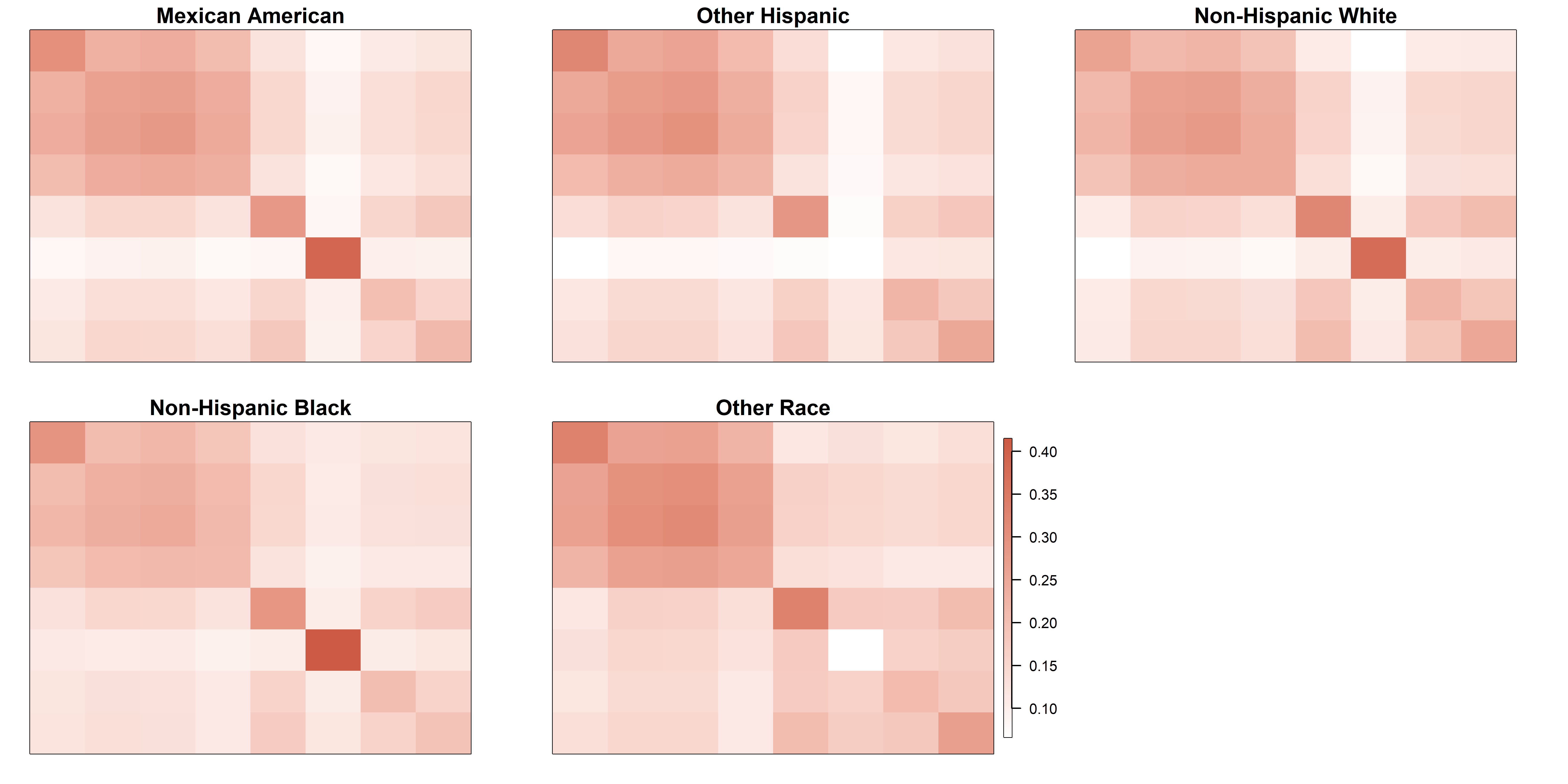
Figure 1: Covariance matrices of the phthalate chemicals across different ethnic groups for NHANES data.

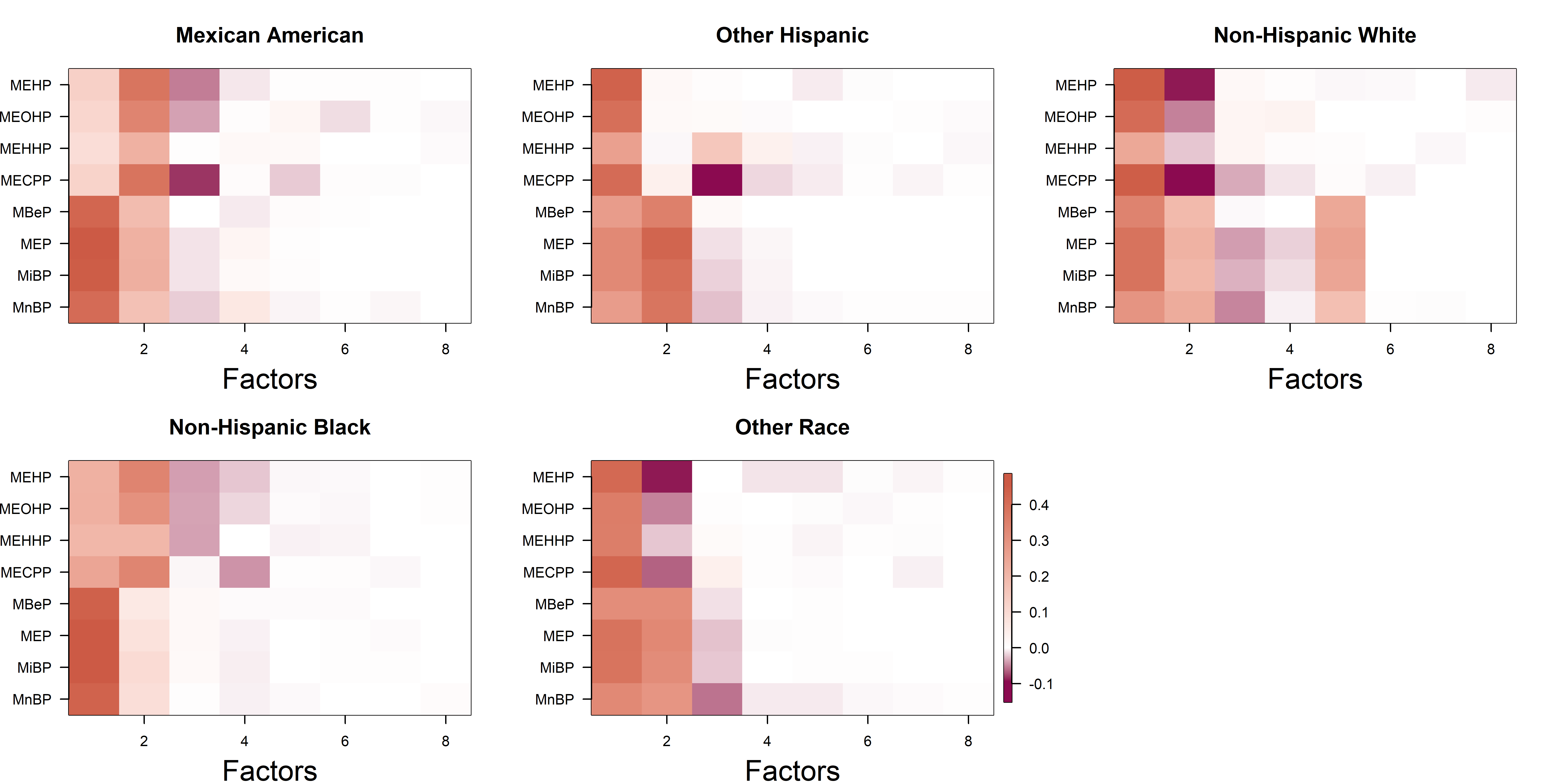
Figure 2: Estimated loadings matrices for different ethnic groups in NHANES based on applying separate Bayesian factor analyses using the approach of Bhattacharya and Dunson (2011).

Fitting the common factor model (1.1) separately for each group, we obtain noticeably different loadings structures as depicted in Figure 2. Throughout the article, including for Figures 1 and 2, we plot matrices using the mat2cols() function for R package IMIFA (Murphy et al., 2020a, b). This function standardizes the color scale across the different matrices. We choose color palettes coral3 and deeppink4 from R package RColorBrewer (Neuwirth, 2014) for positive and negative entries, respectively. Zero entries are white, and the color gradually changes as the value moves away from zero. In the next subsection, we propose a novel approach for multi-group factor analysis to identify common phthalate factors.

2.1 Multi-group model

We have data from multiple groups, with the groups corresponding to individuals in different racial and ethnic categories in NHANES. Each $p$-dimensional mean-centered response $Y_{ij}$, belonging to group $G_{j}$, for $j\in 1:J$ and $i\in 1:n_{j}$, is modeled as:

$$Q_{j}Y_{ij}= \Lambda\eta_{ij}+\epsilon_{ij},$$

$$Q_{j}\sim \mathrm{MN}_{p\times p}(I_{p},U,V),\quad\eta_{ij}\sim\textrm{N}(0,E),$$

$$\epsilon_{ij}\sim \textrm{N}(0,\Sigma).$$ (2.1)

The perturbation matrices $Q_{j}$ are of dimension $p\times p$, and follow a matrix normal distribution, with isotropic covariance $U=V=\alpha I_{p}$. The latent factors $\eta_{ij}$ are heteroscedastic, so that $E$ is diagonal with non-identical entries such that $E=\textrm{diag}(e_{1},\ldots,e_{k})$ with $k$ factors in the model and $\Sigma=\textrm{diag}(\sigma_{1},\ldots,\sigma_{p})$. We discuss advantages of choosing heteroscedastic latent factors in more detail in Section 2.3. After integrating out the latent factors, observations are marginally distributed as $Y_{ij}\sim\textrm{N}(0,Q_{j}^{-1}[\Lambda E\Lambda^{T}+\Sigma](Q_{j}^{-1})^{T})$. If we write $Q_{j}^{-1}=I_{p}+\Psi_{j}$, then $\Lambda$ is the shared loadings matrix, and $\Psi_{j}\Lambda$ is a group-specific loadings matrix. We can quantify the magnitude of perturbation as $\|\Psi_{j}\|_{F}$, where $\|\cdot\|_{F}$ stands for the Frobenius norm. For identifiability of $Q_{j}$’s, we consider $Q_{1}=I_{p}$ and $n_{1}\geq 2$. We call our model Perturbed Factor Analysis (PFA).

2.1.1 Model properties

Let $\Omega_{1}$ and $\Omega_{2}$ be two positive definite (p.d.) matrices. Then there exist non-singular matrices $A$ and $B$, where $\Omega_{1}=AA^{T}$ and $\Omega_{2}=BB^{T}$. By choosing $E=AB^{-1}$, we have $\Omega_{1}=E\Omega_{2}E^{T}$. If the two matrices $\Omega_{1}$ and $\Omega_{2}$ are close, then $E$ will be close to the identity. However, $E$ is not required to be symmetric. In our multi-group model in (2.1), the $Q_{j}$s allow for small perturbations around the shared covariance matrix $H=\Lambda E\Lambda^{T}+\Sigma$. We define the following class for the $Q_{j}$’s,

$$\mathcal{C}_{\epsilon}=\{Q:\|Q-I_{p}\|_{F}\leq\epsilon\}.$$

The index $\epsilon$ controls the amount of deviation across groups. In (2.1) we define $U=V=\alpha I_{p}$, for some small $\alpha$, which we call the perturbation parameter. By choosing $U=V$ to be isotropic covariances, we impose uniform perturbation across all the rows and columns around $I_{p}$. However, the perturbation matrices themselves are not required to be symmetric.

Lemma 1.

$P\big{(}Q_{i}\notin\mathcal{C}_{\epsilon}\big{)}\leq\exp\big{(}-\epsilon^{2}/2\alpha^{2}\big{)}$.

The proof follows from Chebychev’s inequality. This result allows us to summarize the level of induced perturbation for any given $\alpha$. Using this lemma, we can show the following esult

$$\textrm{KL}(\textrm{N}(0,Q_{j}^{-1}[\Lambda E\Lambda^{T}+\Sigma](Q_{j}^{-1})^{T}),\textrm{N}(0,Q_{l}^{-1}[\Lambda E\Lambda^{T}+\Sigma](Q_{l}^{-1})^{T}))$$

$$\quad\lesssim{\big{|}\|Q_{j}^{-1}\|_{F}^{2}-\|Q_{l}^{-1}\|_{F}^{2}\big{|}}.$$

Therefore the Kullback-Leibler divergence between the marginal distributions of any two groups $j$ and $l$ can be bounded by $\big{|}\|Q_{j}^{-1}\|_{F}^{2}-\|Q_{l}^{-1}\|_{F}^{2}\big{|}$ up to some constant. We define a divergence statistic between groups $j$ and $l$ as $d_{jl}=\sqrt{\frac{\big{|}\|Q_{j}^{-1}\|_{F}^{2}-\|Q_{l}^{-1}\|_{F}^{2}\big{|}}{p^{2}}}$. This generates a divergence matrix $D=(\{d_{jl}\})$, where larger $d_{jl}$ implies a greater difference between the two groups.

As in other factor modeling settings, it is important to carefully choose the number of factors. This is simpler for PFA than for other multi-group factor analysis models, because we only need to select a single number of factors instead of separate values for shared and individual-specific components. Indeed, we can directly apply methods developed in the single group setting (Bhattacharya and Dunson, 2011). Due to heteroscedastic latent factors, we can directly use the posterior samples of the loading matrices without applying factor rotation. Computationally, PFA tends to be faster than multi-group factor models such as BMSFA due to a smaller number of parameters, and better identifiability, leading to better mixing of Markov chain Monte Carlo (MCMC).

2.1.2 Choosing the parameter $\alpha$ for multi-group data

The parameter $\alpha$ controls the level of perturbation across groups. We use a cross-validation technique to choose $\alpha$ based on 10 randomly chosen 50-50 splits. We randomly divide each group $50/50$ into training and test sets ten times. Then for a range of $\alpha$ values, we fit the model on the training data and calculate the average predictive log-likelihood of the test set for all the ten random splits. After integrating out the latent factors, the predictive distribution is $Q_{j}Y_{ij}\sim\textrm{N}(0,\Lambda E\Lambda^{T}+\Sigma)$. If there are multiple values of $\alpha$ with similar predictive log-likelihoods, then the smallest $\alpha$ is chosen.

Alternatively, we can take a fully Bayesian approach and put a prior on $\alpha$. We call this method Fully Bayesian Perturbed Factor Analysis (FBPFA). We see that FBPFA performs similarly to PFA in practice, but involves a slightly more complex MCMC implementation. PFA avoids sensitivity to the prior for $\alpha$ but requires the computational overhead of cross validation, ignores uncertainty in estimating $\alpha$, and and can potentially be less efficient in requiring a holdout sample.

2.2 Measurement-error model

We can modify the multi-group model to obtain improved factor estimates in single group analyses by considering observation-level perturbations. Here we observe $Y_{ij}$’s for $j=1,\ldots,m_{i}$, which are $m_{i}$ many proxies of ‘true’ observation $W_{i}$ with multiplicative measurement errors $Q_{ij}^{-1}$’s such that $W_{i}=Q_{ij}Y_{ij}$. The modified model is

$$Q_{ij}Y_{ij}= \Lambda\eta_{i}+\epsilon_{ij},\quad\epsilon_{ij}\sim\textrm{N}(0,\Sigma),$$

$$Q_{ij}\sim \mathrm{MN}_{p\times p}(I_{p},U,V)\quad\eta_{i}\sim\textrm{N}(0,E).$$ (2.2)

In this case, the $Q_{ij}$’s apply a multiplicative perturbation to each data vector. We have $Y_{ij}=Q_{ij}^{-1}W_{i}$ where $Q_{ij}^{-1}$ is a matrix. Thus, here the measurement errors are $U_{ij}=(Q_{ij}^{-1}-I_{p})W_{i}$ and $E(U_{ij}|W_{i})=0$. This model is different from the multiplicative measurement error model of Sarkar et al. (2018). In their paper, observations $Y_{ij}$’s are modeled as $Y_{ij}=W_{i}\circ U_{ij}$, where $\circ$ denotes the element wise dot product and $U_{ij}$’s are independent of $W_{i}$ with $E(U_{ij})=1$. Thus, the measurement error in the $l$-$th$ component (i.e. $U_{ijl}$) is dependent on $W_{i}$ primarily through $W_{il}$. However, in our construction, the measurement errors are a linear function of the entire $W_{i}$.

This is a much more general setup than Sarkar et al. (2018). With this generality comes issues in identifying parameters in the distributions of $Q_{ij}$ and $Y_{ij}$. For simplicity, we again assume $U=V=\alpha I_{p}$. In this case we have,

$$E(Q_{ij}Y_{ij}) =0$$

$$V(Q_{ij}Y_{ij}) =E(V(Q_{ij}Y_{ij}|Q_{ij}))+V(E(Q_{ij}Y_{ij}|Q_{ij}))$$

$$=E(V(Q_{ij}Y_{ij}|Q_{ij}))+0=\alpha^{2}sI_{p}+H,\quad s=\sum_{j=1}^{p}H_{jj}$$

Thus, only the diagonal elements of $H$ are not identifiable and the perturbation parameter $\alpha$ does not influence the dependence structure among the variables. Hence, with our heteroscedastic latent factors, we can still recover the loading structure. To tune $\alpha$, we can use the marginal distributions $Q_{ij}Y_{ij}\sim$N$(0,\alpha^{2}sI_{p}+H)$ to develop a cross validation technique when $m_{i}>1$ for all $i=1,\ldots,n$ as in Section 2.1.2. We split the data into training and testing sets. Then fit the model in the training set and find the $\alpha$ minimizing the predictive log-likelihood in the test set. We can alternatively estimate $\alpha$ as in FBPFA by using a weakly informative prior concentrated on small values, while assessing sensitivity to hyperparameter choice.

2.3 The special case $Q_{j}=I_{p}$ for all $j$

For data within a single group without measurement errors (in the sense considered in the previous subsection), we can modify PFA by taking $Q_{j}=I_{p}$ for all $j$. Then the model reduces to a traditional factor model with heteroscedastic latent factors:

$$Y_{i}= \Lambda\eta_{i}+\epsilon_{i},\quad\epsilon_{i}\sim\textrm{N}(0,\Sigma)$$

$$\eta_{i}\sim \textrm{N}(0,E),$$ (2.3)

where $E$ is assumed to be diagonal with non-identical entries. Integrating out the latent factors, the marginal likelihood is $Y_{i}\sim\textrm{N}(0,\Lambda E\Lambda^{T}+\Sigma)$. Except for the diagonal matrix $E$, the marginal likelihood is similar to the marginal likelihood for a traditional factor model. As $E$ has non-identical diagonal entries, the likelihood is no longer invariant under arbitrary rotations. For the factor model in (1.1), $(\Lambda,\eta)$ and $(\Lambda R,R^{T}\eta)$ have equivalent likelihoods for any orthonormal matrix $R$. This is not the case in our model unless $R$ is a permutation matrix. Thus, this simple modification over the traditional factor model helps to efficiently recover the loading structure. This is demonstrated in Case 1 of Section 5. We also show that the posterior is weakly consistent in the supplementary materials.

3 Prior Specification

As in Bhattacharya and Dunson (2011), we put the following prior on $\Lambda$ to allow for automatic selection of rank and easy posterior computation:

$$\lambda_{lk}|\phi_{lk},\tau_{k}\sim\mathrm{N}(0,\phi_{lk}^{-1}\tau_{k}^{-1}),$$

$$\phi_{lk}\sim\mathrm{Gamma}(\nu_{1},\nu_{1}),\quad\tau_{k}=\prod_{i=1}^{k}\delta_{i}$$

$$\delta_{1}\sim\mathrm{Gamma}(\kappa_{1},1),\quad\delta_{i}\sim\mathrm{Gamma}(\kappa_{2},1)\textrm{ for }i\geq 2.$$

The parameters $\phi_{lk}$ control local shrinkage of the elements in $\Lambda$, whereas $\tau_{k}$ controls column shrinkage of the $k$-$th$ column. We follow the guidelines of Durante (2017) to choose hyperparameters that ensure greater shrinkage for higher indexed columns. In particular, we let $\kappa_{1}=2.1$ and $\kappa_{2}=3.1$, which works well in all of our simulation experiments.

Suppose we initially choose the number of factors to be too large. The above prior will then tend to induce posteriors for $\tau_{k}^{-1}$ in the later columns that are concentrated near zero, leading to $\lambda_{lk}\approx 0$ in those columns. The corresponding factors are then effectively deleted. In practice, one can either leave the extra factors in the model, as they will have essentially no impact, or conduct a factor selection procedure by removing factors having all their loadings within $\pm\zeta$ of zero. Both approaches tend to have similar performance in terms of posterior summaries of interest. We follow the second strategy, motivated by our goal of obtaining a small number of interpretable factors summarizing phthalate exposures. In particular, we apply the adaptive MCMC procedure of Bhattacharya and Dunson (2011) with $\zeta=1\times 10^{-3}$.

For the heteroscedastic latent factors, each diagonal element of $E$ has an independent prior:

$$e_{i}\sim\text{IG}(u,0.1)$$

for some constant $u$. In our simulations, we see that $u$ has minimal influence on the predictive performance of PFA. However, as $u$ increases, more shrinkage is placed on the latent factors. We choose $u=10$ for most of our simulations. For the residual error variance $\Sigma$, we place a weakly informative prior on the diagonal elements:

$$\sigma_{i}\sim\text{IG}(0.1,0.1).$$

In our simulations, a weakly informative IG(0.1,0.1) prior on $\alpha$ works well in terms of both predictive performance and estimation of the loading structure, including in single group analyses.

4 Computation

Posterior inference is straightforward with a Gibbs sampler, because all of the parameters have conjugate full conditional distributions. For the model in (2.1), the full conditional of the perturbation matrix $Q_{j}$ is:

$$\textrm{vec}(Q_{j})|Y\sim\textrm{N}\big{(}\Gamma_{j}(V\otimes U)^{-1}\textrm{vec}(I_{p}),\quad\Gamma_{j}\big{)},$$

where $\Gamma_{j}=\big{[}(V\otimes U)^{-1}+S_{j}\bigotimes H^{-1}\big{]}^{-1}$ and $S_{j}=\sum_{i}Y_{ij}Y_{ij}^{T}$. The notation $\bigotimes$ stands for Kronecker’s product. The full conditionals for all other parameters are described in Bhattacharya and Dunson (2011), replacing $Y_{ij}$ by $Q_{j}Y_{ij}$. For the model in (2.2), the full conditional of $Q_{ij}$ is:

$$\textrm{vec}(Q_{ij})|Y\sim\textrm{N}\big{(}\Gamma_{ij}(V\otimes U)^{-1}\textrm{vec}(I_{p}),\quad\Gamma_{ij}\big{)},$$

where $\Gamma_{ij}=\big{[}(V\otimes U)^{-1}+S_{ij}\bigotimes H^{-1}\big{]}^{-1}$ and $S_{j}=Y_{ij}Y_{ij}^{T}$. Other parameters can again be updated using the results in Bhattacharya and Dunson (2011) replacing $Y_{ij}$ by $Q_{ij}Y_{ij}$. To sample the entire $\textrm{vec}(Q_{ij})$ or $\textrm{vec}(Q_{j})$ together, we need to invert a $p^{2}\times p^{2}$ matrix at each step. Instead we iteratively update the columns of $Q_{ij}$ or $Q_{j}$, which does not require matrix inversion when $U=V=\alpha I_{p}$. For simplicity in notation, we only show the update for the columns in $Q_{j}$ of the model in (2.1). The full conditional of the $l$-$th$ column in $Q_{j}$ is

$$Q_{j,l}|Y\sim\textrm{N}\big{(}M_{l}V_{l},\ V_{l}\big{)},$$

where $V=1/(\sum_{k\in G_{j}}Y_{l,k}^{2}/\textrm{diag}(\Sigma)+1/\alpha)$ and $M_{l}=-\sum_{k\in G_{j}}(Q_{j,-l}Y_{-l,k}-\Lambda\eta_{k})Y_{l,k}/\Sigma+g_{l}/\alpha$, with $\Sigma$ the diagonal error covariance matrix. Here $Q_{j,-l}$ denotes the $p\times(p-1)$ dimensional matrix removing the $l$-$th$ column from $Q_{j}$. Similarly $Y_{-l,k}$ denotes the response of the $k$-$th$ individual from group $G_{j}$, removing the $l$-$th$ variable, and $g_{l}$ the $p$-dimensional vector with one in the $l$-th entry. If we put a prior on $\alpha$, the posterior distribution of $\alpha$ is given by IG$(0.1+(J-1)p^{2},0.1+\sum_{j}\|Q_{j}-I_{p})^{2}\|_{F}^{2})$ for the model in (2.1) and for the model in (2.2), the posterior distribution of $\alpha$ is IG$(0.1+p^{2}\sum_{i}m_{i},0.1+\sum_{ij}\|Q_{ij}-I_{p})^{2}\|_{F}^{2})$. The posterior distribution of $\sigma_{1l}^{2}$ is IG$(0.1+n/2,0.1+\sum_{j=1}^{J}\sum_{k\in G_{j}}(Q_{j}(l,)Y_{kj}-\lambda_{l,}\eta_{kj})^{2}/2)$, where $Q_{j}(l,)$ denotes the $l$-$th$ row of $Q_{j}$. The posterior distribution of $\sigma_{2l}^{2}$ is IG$(0.1+n/2,0.1+\sum_{j=1}^{J}\sum_{k\in G_{j}}\eta_{l,kj}^{2}/2)$.

5 Simulation Study

In this section, we study the performance of PFA in various simulation settings. As ground truth, we consider the two loading matrices given in Figure 3. These are similar to ones considered in Ročková and George (2016). R code to generate the data is provided in the supplementary materials. The two matrices both have 5 columns, the first has 21 rows, and the second has 128 rows. We compare the estimated loading matrices for different choices of the perturbation parameter $\alpha$ and the shape parameter $u$, controlling the level of shrinkage on the diagonal entries of $E$.

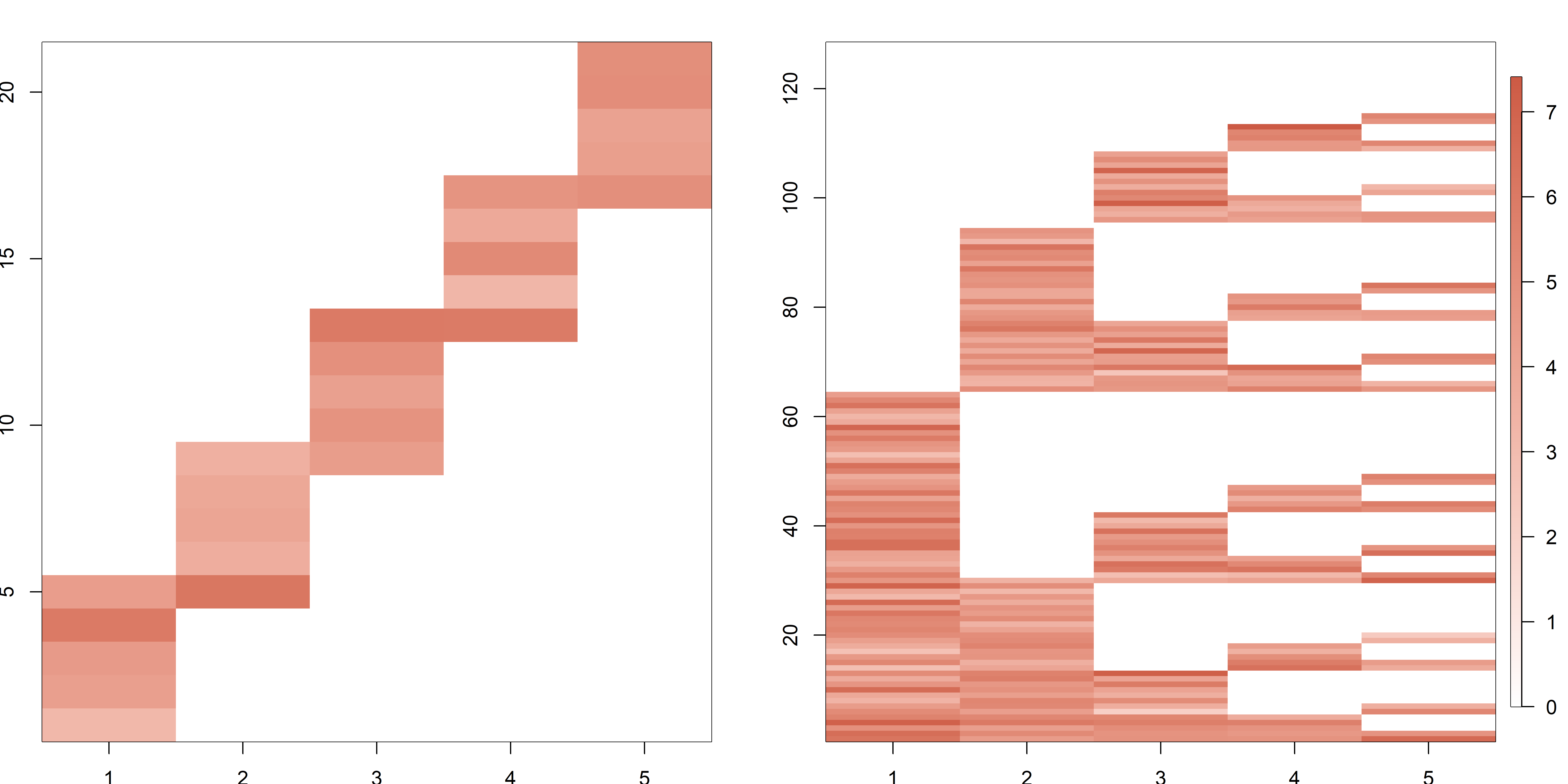
Figure 3: Simulation study true loading matrices of dimension $25$ (Loading 1) and $128\times 5$ (Loading 2), respectively.

For the single group case, we compare with the method of Bhattacharya and Dunson (2011) (B&D), which corresponds to the special case of our approach that fixes the perturbation matrices and latent factor covariances equal to the identity. A point estimate of the loading matrix for B&D is calculated by post-processing the posterior samples. We use the algorithm of Aßmann et al. (2016) to rotationally align the samples of $\Lambda$, as in De Vito et al. (2018). In contrast, our method uses the post-processing algorithm of Roy et al. (2019). For the multi-group case, we compare our estimates with Bayesian Multi-Study Factor Analysis (BMSFA). We use the MSFA package at https://github.com/rdevito/MSFA.

We compare the different methods using predictive log-likelihood. Simulated data are randomly divided $50/50$ into training and test sets. After fitting each model on the training data, we calculate the predictive log-likelihood of the test set. All methods are run for $7000$ iterations of the Gibbs sampler, with $2000$ burn-in samples. Each simulation is replicated $30$ times.

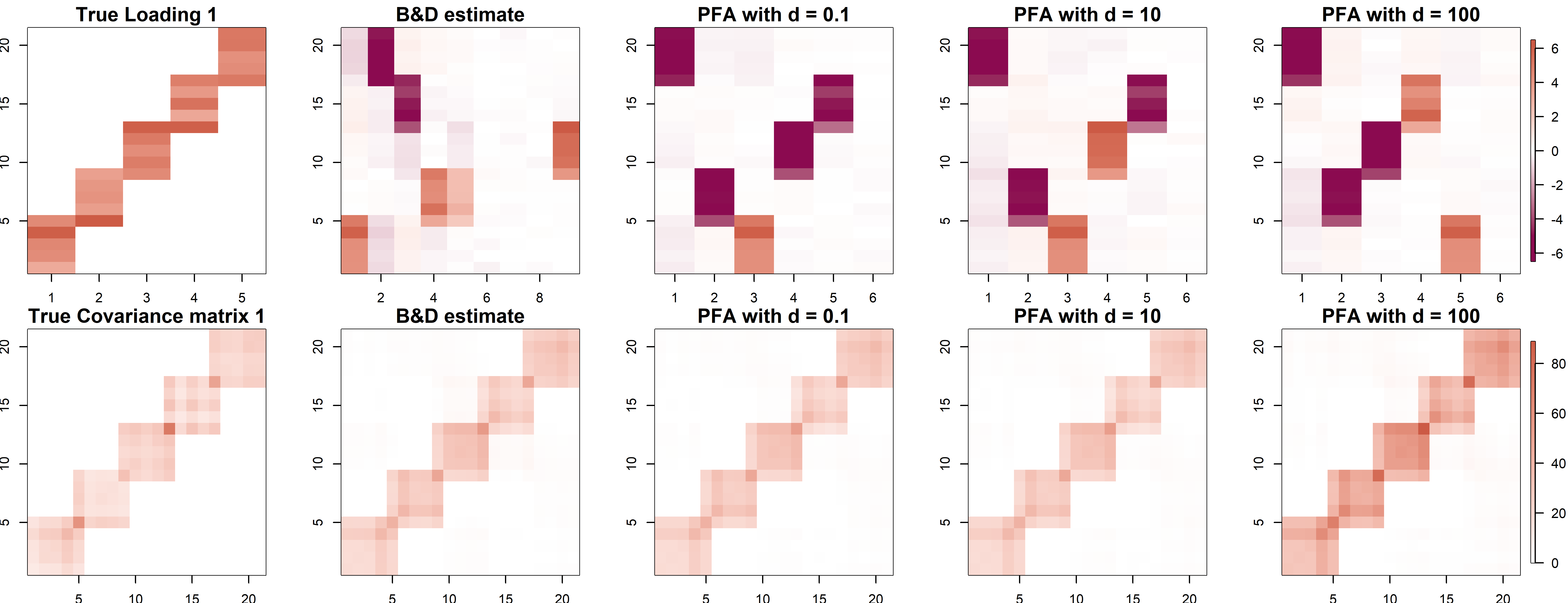
Figure 4: Comparison of true and estimated loading matrices and covariance matrices for case $1$. Comparison of B&D FA with our method for different choices of $u$. Results for loading matrix 1 are in (a) and 2 in (b). For all the cases, we fix $Q_{j}=I$.The color gradient added in the last image of each row holds for all the images in that row.

5.1 Case 1: Single group, $Q_{j}=I_{p}$

We first consider single group factor analysis. Starting with the two loading matrices in Figure 3, we simulate latent factors from $\textrm{N}(0,I_{5})$, and generate datasets of $500$ observations, with residual variance $\Sigma=I_{5}$. We compare B&D with our method when $Q_{j}=I_{5}$, so the only adjustment is to use heteroscedastic latent factors. Note that the simulated latent factors actually have identical variances.

Table 3: MSE of estimated covariance matrix for loading matrix $1$, across different values of $u$

$u$	MSE
0.1	1.04
10	1.32
100	1.38

In Tables 3 and 4, we compare methods by MSE of the estimated versus true covariance matrix. For the loading matrix $1$, B&D had an MSE of $2.59$, which is dominated by our method across a range of values of $u$.

Table 4: MSE of estimated covariance matrix for loading matrix $2$, across different values of $u$

$u$	MSE
0.1	5.21
10	9.45
100	10.32

For the loading matrix $2$, B&D had an MSE of $10.81$. Again, our method beats this across a range of values of $u$. The B&D model is a special case of PFA with $E=I_{p}$ in (2.3). We conjecture that the gains seen for PFA are due to the more flexible induced shrinkage structure on the covariance matrix.

We compare the estimated and true loading matrices in Figure 4. Throughout the paper, PFA estimated loadings are based on $\hat{\Lambda}\hat{E}^{1/2}$, where $\hat{\Lambda}$ and $\hat{E}$ are the estimated loading and covariance matrix of the factors, respectively. This makes the loadings comparable to methods that use identity covariance for the latent factors. PFA performs overwhelmingly better at estimating the true loading structure compared with B&D FA. The first five columns of the estimated loadings based on PFA are very close to the true loading structure under some permutation. This gain over B&D may be due to a combination of the more flexible shrinkage structure and the different post-processing scheme. On comparing $\hat{\Lambda}\hat{E}^{1/2}$ for different choices of $u$, we see that the estimates are not sensitive to the hyperparameter $u$. Estimation MSE is better for smaller $u$, but the general structure of the loadings matrix is recovered accurately for all $u$.

5.2 Case 2: Multi-group, multiplicative perturbation

In this case, we simulate data from the multi-group model in (2.1) for $i=1,\ldots,500$. Observations $Y_{i}$ are first generated using the same method as in case 1. The data are then split into $10$ groups of $50$ observations, such that $G_{j}=\{Y_{k}:50(j-1)\leq k\leq 50j\}$ for $j=1,\ldots,10$. The groups are perturbed using matrices $Q_{j0}\sim$MN$(I_{p},\alpha_{0}I_{p},\alpha_{0}I_{p})$ for different choices of $\alpha_{0}$, setting $Q_{1}=I_{p}$.

Figure 5: Comparison of estimated loading matrix 1 in simulation case 2 with different choices of $\alpha_{0}$ and $\alpha$ where $Q_{j0}\sim$MN$(I_{p},\alpha_{0}I_{p},\alpha_{0}I_{p})$ and $U=\alpha I_{p}=V.$ (a) $\alpha=10^{-4},\alpha_{0}=10^{-4}$, (b) $\alpha=10^{-2},\alpha_{0}=10^{-4}$, (c) FBPFA with $\alpha_{0}=10^{-4}$, (d) BMSFA with $\alpha_{0}=10^{-4}$, (e) $\alpha=10^{-4},\alpha_{0}=10^{-2}$, (f) $\alpha=10^{-2},\alpha_{0}=10^{-2}$, (g) FBPFA with $\alpha_{0}=10^{-2}$, (h) For BMSFA with $\alpha_{0}=10^{-2}$. True loading matrices are plotted twice in columns 1 for easier comparison with other images.

Figure 5 shows the estimated loading matrices. We obtain accurate estimates even when assuming a higher level of perturbation than the truth, $\alpha_{0}\leq\alpha$. However, the estimates are best when $\alpha=\alpha_{0}=10^{-4}$. Performance degrades more sharply when we underestimate the level of perturbation, as in the case where $\alpha=10^{-4},\alpha_{0}=10^{-2}$. The BMSFA code requires an upper bound on the number of shared and group-specific factors; we choose both to be $6$. The estimated loadings from PFA and FBPFA are better than BMSFA. Except for cases with a higher level of perturbation using BMSFA, the estimated loadings matrix is close to the truth under some permutation of the columns. BMSFA estimated loadings usually are of lower magnitude, which may be due to the additive structure of the model. Thus they look faded in almost all the figures. The cumulative shrinkage prior used in PFA and BMSFA induces continuous shrinkage instead of exact sparsity, but nonetheless does a good job overall of capturing the true sparsity pattern. BMSFA estimated loadings for $\alpha_{0}=10^{-2}$ look blank as the estimated loading has all entries near zero. Results for the case 2 loading structure are shown in Figure 5 of the Supplementary materials.

Table 5: Average predictive log-likelihood for PFA with optimal $\alpha$, FBPFA and BMSFA in simulation case 2.

True Loading	$\alpha_{0}$	PFA for optimal $\alpha$	FBPFA	BMSFA
Loading 1	$10^{-4}$	$-$31.65	$-25.92$	$-$679.36
	$10^{-2}$	$-$30.32	$-26.01$	$-$921.76
Loading 2	$10^{-4}$	$-$210.43	$-251.13$	$-$6871.38
	$10^{-2}$	$-$351.42	$-$304.10	$-$25018.50

We also apply the same simulation setting with higher error variances. Figure 6 compares the estimated loadings. All the methods identify the true structure when the residual standard deviation is 5, but only PFA with correctly specified $\alpha$ produces good estimates when we increase it to 10.

Figure 6: Comparison of estimated loading matrices in simulation case 2 with increasing error variances and $\alpha_{0}=10^{-4}$: (a) $\alpha=10^{-4}$ with error variance 25, (b) $\alpha=10^{-4}$ with error variance 100, (c) BMSFA with error variance 25, (d) BMSFA with error variance 100, (e) FBPFA with error variance 25, (f) FBPFA with error variance 100.

In Figure 7, we show the predictive log-likelihood averaged over all the splits under a range of $\alpha$ values. For each choice of $\alpha$, we fit the model to a training set and calculate the predictive log-likelihood on a test set for 10 randomly chosen training-test splits. This demonstrates the utility of our cross-validation technique in finding the optimal $\alpha$. In Table 5, we compare the performance of PFA with optimal $\alpha$, FBPFA, and BMSFA in terms of predictive likelihood. PFA and FBPFA have overwhelmingly better performance. We also show the range of predictive log-likelihoods for each choice of $\alpha$ in Figure 7 using dotted red lines. FBPFA is better at recovering the true loading structure for $p=21$, but for the higher dimensional case with $p=128$ PFA tends to be better.

Figure 7: Average predictive log-likelihoods in black along with two dotted red lines, denoting the range of predictive log-likelihoods across all the splits for different choices of $\alpha$ in simulation case 2 for two cases - in the first case the perturbation matrices are generated using true $\alpha_{0}=10^{-2}$ and in the second case $\alpha_{0}=10^{-4}$. This is based on the simulation experiment of Figure 5.

5.2.1 Case 2.1: Partially shared factors

We also repeat the case 2 simulation but modified to accommodate a partially shared structure. In particular, we generated the data as in case 2 but for the last two groups we let $Q_{j}Y_{i}\sim$N$(\Lambda_{01}\Lambda_{01}^{T}+I_{p})$ for $i\in G_{j}$ and $j=9,10$. Here $\Lambda_{01}=\Lambda_{0}[,1:3]$ is a $p\times 3$ dimensional matrix having the first three columns from $\Lambda_{0}$. The choices for $\Lambda_{0}$ are given in Figure 3.

Figure 8: Comparison of estimated loading in the partially shared modification of simulation case 2. Row 1 corresponds to true loading structure 1 and row 2 to true loading structure 2. (a) FBPFA with $\alpha_{0}=10^{-4}$, (b) FBPFA with $\alpha_{0}=10^{-2}$, (c) BMSFA with $\alpha_{0}=10^{-4}$, (d) BMSFA with $\alpha_{0}=10^{-2}$.

The estimated loading matrices are compared in Figure 8 for two levels of perturbations, $\alpha_{0}=10^{-4},10^{-2}$. FBPFA works well for any level of perturbation, while BMSFA works well for only the lower perturbation level. The estimated loading in Figure 8 (d) looks blank due to near zero entries. Estimated loadings for the case 2 loading structure are in Figure 6 of the Supplementary materials.

5.3 Case 3: Multi-group factor model

In this case, we generate data from the Bayesian multi-study factor analysis (BMSFA) model as in De Vito et al. (2018).

$$Y_{i}= \Lambda\eta_{i1}+\Psi_{j}\eta_{i2}+\epsilon_{1i}\textrm{ and }Y_{i}\in G_{j},$$

$$\epsilon_{1i}\sim \textrm{N}(0,\Sigma)\quad\eta_{i1},\eta_{i2}\sim\textrm{N}(0,I_{p}),$$ (5.1)

where the group-specific loadings ($\Psi_{j}$’s) are lower in magnitude in comparison to the shared loading matrix $\Lambda$. We generate the $\Psi_{j}$s from N$(-0.5,0.8)$. These $\Psi_{j}$ matrices are the same dimension as the shared loading matrix $\Lambda$.

Table 6: Average predictive log-likelihood for PFA for different choices of $\alpha$, FBPFA and BMSFA in Simulation Case 3.

Generative	True	PFA for	PFA for	FBPFA	BMSFA
Distribution	Loading	$\alpha=10^{-2}$	$\alpha=10^{-4}$
of $\Psi_{j}$’s
N$(-0.2,0.2)$	Loading 1	$-$33.41	$-$44.10	$-$26.16	$-$500.66
	Loading 2	$-$336.58	$-$259.79	$-$265.77	$-$9547.77
N$(-0.5,0.8)$	Loading 1	$-$49.25	$-$53.32	$-$37.89	$-$720.35
	Loading 2	$-$584.82	$-$308.72	$-$1003.02	$-$14187.36

Figure 9 compares the estimated loadings with the true shared loadings across different methods: PFA for two different perturbation parameters, FBPFA and BMSFA. Although we generate the data from BMFSA, all the estimates are very much comparable in Figure 9. However, PFA and FBPFA again outperform BMSFA in terms of predictive log-likelihoods as shown in Table 6. In the supplementary material, we present another simulation setting akin to BMSFA. There, the data generating process is similar to BMSFA with minor modifications in the shared and group-specific loading structures. Estimated loadings for the case 2 loading structure are in Figure 7 of the Supplementary materials.

Figure 9: Comparison of estimated loading matrices in simulation case 3 when the true data generating process follows the model in (5.1). (a) PFA with $\alpha=10^{-4}$, (b)PFA with $\alpha=10^{-2}$, (c) FBPFA, (d) BMSFA.

5.4 Case 4: Mimic NHANES data

In this section, we generate data from the model in (2.1). However, the model parameters $Q_{j}$’s and $\Lambda$ are first estimated on the NHANES data with $\alpha=10^{-2}$. Then, based on these estimated parameters, we generate the data following the same model. Figure 10 compares the estimated loadings across all the methods: PFA for different choices of $\alpha$, FBPFA, and BMSFA. We find that all the methods recover loading structures that match with our estimated loadings from Section 6. For PFA and FBPFA, we selected the number of factors as described in Section 3, and hence these approaches produced fewer columns than BMSFA.

Figure 10: Comparison of estimated loading matrices in simulation case 4 where the true loading matrix is PFA estimated loading with $\alpha=10^{-2}$ for mean-centered NHANES data and the data are simulated from the model (2.1). (a) PFA with $\alpha=10^{-2}$, (b) PFA with $\alpha=10^{-4}$, (c) FBPFA, (d) BMSFA. The color gradient added in the last image holds for all the images.

6 Application to NHANES data

We fit our model in (2.1) to the NHANES dataset as described in Section 2 to obtain phthalate exposure factors for individuals in different ethnic groups. Before analysis the mean chemical levels across all groups are subtracted to mean-center the data. The data are then randomly split, with $2/3$ in each group as a training set, and $1/3$ as a test set. We collect 5000 MCMC samples after a burn-in of 5000 samples. Convergence is monitored based on the predictive log-likelihood of the test set at each MCMC iteration. The hyperparameters are the same as those in Section 5. The predictive log-likelihood of the test data are used to tune $\alpha$ as described in Section 2.1.2. Based on our cross-validation technique, $\alpha=10^{-2}$ is chosen. Note that our final estimates are based on the complete data. Our BMSFA implementation sets the upper bounds at 8 for both shared and group-specific factors. Figure 4 of the supplementary materials depicts trace plots of the loading and perturbation matrices for FBPFA.

Figure 11 shows the estimated loadings using PFA, FBPFA, and BMSFA. All plots show two significant factors, with some suggestions of a third factor. For PFA and FBPFA, all the chemicals load on the first factor, and the second factor is loaded on by the first four chemicals, namely MEHP, MEOHP, MEHHP, and MECPP. Figure 1 also suggests that these four chemicals are related to each other more than the others. This is not surprising, as MECPP, MEHHP, and MEOHP are oxidative metabolities of MEHP.

Comparing the predictive log-likelihoods for PFA, FBPFA and BMSFA, we obtain values of $4.12$, $5.02$ and $-7.99$, respectively, suggesting much better performance for the PFA-based approaches. As an alternative measure of predictive performance, we also consider test sample MSE using 2/3 of the data as training and 1/3 as test. The predictive value of the test data is estimated by averaging the predictive mean conditionally on the parameters and training data over samples generated from the training data posterior. We obtain predictive MSE values of $0.05$ and $0.09$ for PFA with $\alpha=10^{-4}$ and $\alpha=10^{-2}$, respectively. FBPFA yields a value of $0.14$, while BMSFA has a much larger error of $0.70$. Considering that the data are normalized before analysis, the naive prediction that sets all the values to zero would yield an MSE of $1.0.$

Figure 11: Comparison of estimated loading matrices with different methods. PFA estimates are based on $\alpha=10^{-2}$.

To explore similarities across groups, we calculate divergence scores and create the divergence matrix $D$. This matrix is provided in Table 7. To summarize $D$, we also provide a network plot between different groups in Figure 12. The plot uses greater edge widths between ethnic groups when the divergence statistic between the groups is small. In particular, the edge width between two nodes $(j,l)$ is calculated as $60/d_{jl}$. Thicker edges imply greater similarity. This figure implies that non-Hispanic whites differ the most in phthalate exposure profiles from the other groups, supporting the findings of our exploratory ANOVA analysis in the Section 3 of the supplementary materials and findings in the prior literature (Bloom et al., 2019). We find evidence of one extra factor among non-Hispanic whites relative to the other groups in Figure 2. The two Hispanic ethnicity groups are very similar in loadings as shown in Figure 2 and also their Hotelling $T^{2}$ distance is relatively small in Table 2. These results support our preliminary analysis, described in Section 2.

In Table 8, we show square norm differences between the group-specific loadings, estimated using BMSFA.The $(i,j)$-$th$ entry of the table is calculated as $\sqrt{\sum_{lk}(A_{ill}-A_{jlk})^{2}}$, where the matrices $A_{i}$ and $A_{j}$ are the estimated group-specific loadings for the groups $i$ and $j$, respectively, using BMSFA. Based on these results, BMSFA-based inferences on differences in exposure profiles across ethnic groups are noticeably different from our PFA-based results reported above. In particular, all the groups seem to be approximately the same distance apart. The results using BMSFA from Table 8 are not consistent with Hotelling $T^{2}$-based our exploratory data analysis results from Table 2 and PFA-based results from Table 7.

Table 7: Estimated divergence scores for different pairs of ethnic groups based on NHANES data.

	Mex	OH	N-H White	N-H Black	Other/Multi
Mex	0.00	5.86	41.35	10.22	3.82
OH	5.86	0.00	40.93	8.38	4.45
N-H White	41.35	40.93	0.00	40.06	41.17
N-H Black	10.22	8.38	40.06	0.00	9.48
Other/Multi	3.82	4.45	41.17	9.48	0.00

Figure 12: Network plot summarizing similarity between ethnic groups based on the divergence metric with thicker edges implying smaller divergence scores. Nodes correspond to different ethnic groups.

Table 8: Square norm difference of the group-specific loadings, estimated using BMSFA.

	Mex	OH	N-H White	N-H Black	Other/Multi
Mex	0.00	0.75	0.70	0.59	0.78
OH	0.75	0.00	0.63	0.75	0.73
N-H White	0.70	0.63	0.00	0.68	0.84
N-H Black	0.59	0.75	0.68	0.00	0.91
Other/Multi	0.78	0.73	0.84	0.91	0.00

7 Discussion

In this paper, our focus has been on identifying a common set of phthalate exposure factors that hold across different ehtnic groups, while also inferring differences in exposure profiles across groups. To accomplish this goal, we focused on data from NHANES, which contain rich information on ethnicity and exposures. We found that our proposed perturbed factor analysis (PFA) approach had significant advantages over existing approaches in addressing our goals.

There are multiple important next steps to consider to expand on our analysis. A first is to include covariates. In addition to phthalates and ethnic group data, NHANES collects information that may be relevant to understanding ethnic differences in exposure profiles, including BMI, age, socioeconomic status, gender and other factors. Li and Jung (2017) consider a related problem of incorporating covariates into factor models for multiview data. Perhaps the simplest and most interpretable modification of our PFA model of the NHANES data is to allow the factor scores $\eta_{ij}$ to depend on covariates $X_{ij}=(1,X_{ij2},\ldots,X_{ijq})^{T}$ through a latent factor regression. For example, we could let $\eta_{ij}=\beta X_{ij}+\xi_{ij}$, with $\beta$ a $k\times q$ matrix of coefficients and $\xi_{ij}\sim\textrm{N}(0,E).$

Another important direction is to extend the analysis to allow inferences on relationships between exposure profiles and health outcomes. NHANES contains rich data on a variety of outcomes that may be adversely affected by phthalate exposures. To include these outcomes in our analysis, and effectively extend PFA to a supervised context, we can define separate PFA models for the exposures and outcomes, with these models having shared factors $\eta_{ij}$ but different perturbation matrices. It is straightforward to modify the Gibbs sampler used in our analyses to this case and/or the extension described above to accommodate covariates $X_{ij}$; further modifications to mixed continuous and categorical variables can proceed as in Carvalho et al. (2008); Zhou et al. (2015) with the perturbations conducted on underlying variables. Relying on such a broad modeling and computational framework, it would be interesting to attempt to infer causal relationships between ethnicity and phthalates and adverse health outcomes. Mediation analysis may provide a useful framework in this respect.

Beyond this application, the proposed PFA approach may prove useful in other contexts. The important features of PFA include both the incorporation of a multiplicative perturbation of the data and the use of heteroscedastic latent factors. These innovations are potentially useful beyond the multiple group setting to meta analysis, measurement error models, nonlinear factor models including Gaussian process latent variable models (Lawrence, 2004; Lawrence and Candela, 2006) and variational auto-encoders (Kingma and Welling, 2014; Pu et al., 2016), and even to obtaining improved performance in ‘vanilla’ factor modeling lacking hierarchical structure.

Code is available for implementing the proposed approach and replicating our results from Section 5.2 at https://github.com/royarkaprava/Perturbed-factor-model.

8 Acknowledgments

This research was partially supported by grant R01-ES027498 from the National Institute of Environmental Health Sciences (NIEHS) of the National Institutes of Health (NIH). We would like to thank Roberta De Vito for sharing her source code of the Bayesian MSFA model. We would also like to thank Noirrit Kiran Chandra for his feedback on the code which heavily improved its usage both in low and high-dimensional settings.

9 Supplementary Materials

9.1 Posterior consistency

Let $\Theta_{\Lambda},\Theta_{\Sigma},\Theta_{E}$ be the parameter spaces of $\Lambda,\Sigma$ and $E$, respectively, $\Theta$ be the set of $p\times p$ positive semidefinite matrices corresponding to the parameter space of $H$, and $\mathcal{Q}_{j}$ be the parameter space of $Q_{j}$. Let $\Pi_{\Lambda},\Pi_{\Sigma},\Pi_{E},\Pi_{Q}$ be the priors for $\Lambda,\Sigma,E$ and $Q_{j}$’s. We restate some of the results from Bhattacharya and Dunson (2011) for our modified factor model. With minor modification, the proofs will remain the same.

Let $g:\Theta_{\Lambda}\times\Theta_{\Sigma}\times\Theta_{E}\rightarrow\Theta_{H}$ be a continuous map such that $g(\Lambda,\Sigma,E)=\Lambda^{T}E\Lambda+\Sigma$.

Lemma 2.

For any $(\Lambda,\Sigma,E)\in\Theta_{\Lambda}\times\Theta_{\Sigma}\times\Theta_{E}$, we have $g(\Lambda,\Sigma,E)\in\Theta_{H}$.

The proof is similar to Lemma 1 of Bhattacharya and Dunson (2011). In our Bayesian approach, we choose independent priors for $\Lambda$, $\Sigma$ and $E$ and that induces a prior on $H$ through the map $g$. We also have following proposition.

Proposition 3.

If $(\Lambda,\Sigma,E)\sim\Pi_{\Lambda}\otimes\Pi_{\Sigma}\otimes\Pi_{E}$, then $\Pi_{\Lambda}\otimes\Pi_{\Sigma}\otimes\Pi_{E}(\Theta_{\Lambda}\times\Theta_{\Sigma}\times\Theta_{E})=1$.

The proof is similar to Proposition 1 of Bhattacharya and Dunson (2011) with minor modifications. Now, we proceed to establish that the posterior of our multigroup model is weakly consistent under a fixed $p$ and increasing $n$ regime. Let us assume that the complete parameter space is $\kappa=(\Lambda,\Sigma,E,Q_{2},\ldots,Q_{j})$ and let $\kappa_{0}$ be the truth for $\kappa$.

Assumptions:

1. For some $M>0$, the true perturbation matrices are $Q_{j0}\in\mathcal{C}_{M}$, with $\mathcal{C}_{M}$ defined in Section 2.1.1.

2. There exists some $E>0$, $F_{1}>0$ and $F_{2}>0$ such that $\max_{ij}|\Lambda_{0}|<E$ and $F_{1}<e_{0k}<F_{2}$ for all $k=1,\ldots r$.

Theorem 4.

Under Assumptions 1-2, the posterior for $\kappa$ is weakly consistent at $\kappa_{0}$.

We first show that our proposed prior has large support in the sense that the truth belongs to the Kullback-Leibler support of the prior. Thus the posterior probability of any neighbourhood around the truth converges to one in $P_{\kappa_{0}}^{(n)}$-probability as $n$ goes to $\infty$ as a consequence of Schwartz (1965). Here $P_{\kappa}^{(n)}$ is the distribution of a sample of $n$ observations with parameter $\kappa$. Hence, the posterior is weakly consistent.

Proof.

For $q,q^{*}\in$ the space of probability measure $\mathcal{P}$, let the Kullback-Leibler divergences be given by

$$KL(q^{*},q)=\int q^{*}\log{\frac{q^{*}}{q}}.$$

Let $K(\kappa_{0},\kappa)$ denote the Kullback-Leibler divergence

$$\sum_{j=1}^{J}KL(\textrm{N}(0,Q_{j}^{-1}[\Lambda E\Lambda^{T}+\Sigma](Q_{j}^{T})^{-1}),\textrm{N}(0,Q_{j0}^{-1}[\Lambda_{0}E_{0}\Lambda_{0}^{T}+\Sigma_{0}](Q_{j0}^{-1})^{T})).$$

For our model, we have

$$K(\kappa_{0},\kappa) =\frac{1}{2n}\Bigg{[}\sum_{j=1}^{J}-n_{j}\log|Q_{j0}^{-1}H_{0}(Q_{j0}^{T})^{-1}\{Q_{j}^{-1}H(Q_{j}^{T})^{-1}\}^{-1}|$$

$$\quad+n_{j}\textrm{tr}\big{(}Q_{j0}^{-1}H_{0}(Q_{j0}^{T})^{-1}\{Q_{j}^{-1}H(Q_{j}^{T})^{-1}\}^{-1}-I_{p}\big{)}\Bigg{]}$$

To prove Theorem 4, we rely on the following Lemma.

Lemma 5.

For any $\epsilon>0$, there exists $\epsilon_{1}>0,\epsilon_{2}>0$, and $\epsilon_{3j}>0$ for $j\in\{2,\ldots,J\}$ such that $\|\Lambda-\Lambda_{0}\|_{F}^{2}\leq\epsilon_{1}^{2}$, $\|E-E_{0}\|_{F}^{2}\leq\epsilon_{2}^{2}$ and $\|Q_{j}-Q_{j0}\|_{F}^{2}\leq\epsilon_{3j}^{2}$, then we have

$$\Pi\big{\{}K(\kappa_{0},\kappa)\leq\epsilon\big{\}}\geq$$

$$\quad\Pi\big{\{}\|\Lambda-\Lambda_{0}\|_{F}^{2}\leq\epsilon_{1}^{2},\|E-E_{0}\|_{F}^{2}\leq\epsilon_{2}^{2},\|Q_{j}-Q_{j0}\|_{F}^{2}\leq\epsilon_{3j}^{2},j=2,\ldots,J\big{\}}$$

Due to continuity of the functions such as determinant, trace and $g(\cdot)$, the above result is immediate following the proof of Theorem 2 in Bhattacharya and Dunson (2011). For our proposed priors, the prior probability of the R.H.S. of Lemma 5 is positive. Thus the prior probability of any Kullback-Leibler neighborhood around the truth is positive. This proves Theorem 4. ∎

9.2 Additional simulations

9.2.1 Case 1: Multi-group, additive perturbation

In Section 5.2 of the manuscript, each group is multiplied by a unique perturbation matrix $Q_{j}$. In this case, we perturb the data by adding a group-specific loading matrix $\Psi_{j}$ to a shared loading matrix $\Lambda$, as in model (9.1).

$$Y_{i}= (\Lambda+\Psi_{j})\eta_{i}+\epsilon_{1i}\textrm{ and }Y_{i}\in G_{j},$$

$$\epsilon_{1i}\sim \textrm{N}(0,\Sigma)\quad\eta_{i}\sim\textrm{N}(0,I_{p}),$$ (9.1)

where the group-specific loadings ($\Psi_{j}$’s) are lower in magnitude in comparison to the shared loading matrix $\Lambda$. This can also be an alternative perturbation model. The group-specific loadings are generated in Figure 13 which shows the true and estimated loading matrices from BMFSA, FBPFA, and PFA across a range of values of $\alpha$. The estimated loadings from PFA are much closer to the truth than BMFSA. We find that the estimated loading matrices are some permutation of the true loading matrix with some exceptions. For the case with higher perturbation (row 2 of Figure 13), BMSFA estimate is not good and PFA estimate is also bad for lower values of $\alpha$. Similarly, for the case with lower perturbations, PFA estimate with lower $\alpha$ is better than higher $\alpha$ estimated loading. Table 9 compares predictive likelihoods of the two methods in different cases, and again, PFA and FBPFA outperform BMSFA.

Figure 13: Comparison of estimated loading matrices in Simulation case 9.2.1 when the true data generating process follows the model in (9.1). For the first two rows, true $\Psi_{j}$’s are generated from N$(-0.2,0.2)$ and for the last two rows $\Psi_{j}$’s are generated from N$(-0.5,0.8)$ and for each row (a) PFA with $\alpha=10^{-4}$, (b) PFA with $\alpha=10^{-2}$, (c) FBPFA, (d) BMSFA

Table 9: Average predictive log-likelihood for PFA for different choices of $\alpha$, FBPFA and BMSFA in Simulation Case 1.

Generative	True	PFA for	PFA for	FBPFA	BMSFA
Distribution of $\Psi_{j}$’s	Loading	$\alpha=10^{-2}$	$\alpha=10^{-4}$
N$(-0.2,0.2)$	Loading 1	$-56.27$	$-60.71$	$-56.63$	$-$429.28
	Loading 2	$-1041.28$	$-361.82$	$-421.28$	$-$5853.65
N$(-0.5,0.8)$	Loading 1	$-$30.68	$-$50.09	$-54.62$	$-$514.67
	Loading 2	$-$320.04	$-$246.06	$-479.59$	$-$6798.37

9.2.2 Case 2: Observation-level perturbations

In this case, we generate data from the model (2.2). First, a non-perturbed dataset is generated exactly the same way as in Section 5.1 and 5.2 in the manuscript. Then, we generate separate perturbation matrices $Q_{i0}\sim\text{MN}(I_{p},\alpha_{0}I_{p},\alpha_{0}I_{p})$ for each data vector $Y_{i}$. We repeat this simulation for different choices of $\alpha_{0}$.

Figure 14: Estimated loadings using PFA for different choices of $\alpha$ in Simulation case 9.2.2 for $\alpha_{0}=10^{-4}$ and two loadings. (a): Estimated loading for $\alpha=10^{-2}$, (b): For $\alpha=10^{-4}$, (c): For $\alpha=10^{-5}$.

Figure 15: Estimated loadings using FBPFA for different choices of $\alpha_{0}$ in Simulation case 9.2.2 for two cases and two loadings. (a): Estimated loading for $\alpha_{0}=10^{-4}$, (b): For $\alpha_{0}=10^{-2}$.

Figures 14 shows the estimated loading when they are estimated using $\alpha=10^{-4}$. The method performs poorly when the perturbation parameter $\alpha$ is lower than the true parameter $\alpha_{0}$ as in the previous cases. Figure 15 illustrates the performance of FBPFA in this case. When the perturbation is higher, the performance deteriorates as it is more difficult to capture the loading structure accurately. Overall, our method is able to accurately estimate the true loading structure under some permutation of the columns.

9.2.3 More exploratory analysis on NHANES data

For each chemical level, we fit an one-way ANOVA model to analyse group-specific effects on each phthalate level separately. The results are provided from Table 10 to 17.

Table 10: Estimated group effects from a one-way ANOVA analysis for the phthalate MnBP.

	Estimate	Std. Error	t value	Pr($>|t|$)
(Intercept)	3.85	0.11	36.27	0.00
N-H Black	0.36	0.15	2.33	0.02
N-H White	-0.29	0.13	-2.26	0.02
OH	0.46	0.18	2.55	0.01
Other/Multi	-0.09	0.22	-0.41	0.68

Table 11: Estimated group effects from a one-way ANOVA analysis for the phthalate MiBP.

	Estimate	Std. Error	t value	Pr($>|t|$)
(Intercept)	2.88	0.06	49.23	0.00
N-H Black	0.59	0.08	6.97	0.00
N-H White	-0.35	0.07	-4.98	0.00
OH	0.33	0.10	3.28	0.00
Other/Multi	-0.08	0.12	-0.68	0.50

Table 12: Estimated group effects from a one-way ANOVA analysis for the phthalate MEP.

	Estimate	Std. Error	t value	Pr($>|t|$)
(Intercept)	8.32	0.29	28.80	0.00
N-H Black	2.84	0.42	6.79	0.00
N-H White	-1.41	0.35	-4.02	0.00
OH	1.18	0.49	2.40	0.02
Other/Multi	-0.99	0.60	-1.64	0.10

Table 13: Estimated group effects from a one-way ANOVA analysis for the phthalate MBeP.

	Estimate	Std. Error	t value	Pr($>|t|$)
(Intercept)	2.79	0.07	39.90	0.00
N-H Black	0.27	0.10	2.66	0.01
N-H White	-0.09	0.08	-1.05	0.29
OH	-0.01	0.12	-0.06	0.95
Other/Multi	-0.23	0.15	-1.57	0.12

Table 14: Estimated group effects from a one-way ANOVA analysis for the phthalate MECPP.

	Estimate	Std. Error	t value	Pr($>|t|$)
(Intercept)	4.80	0.12	41.52	0.00
N-H Black	-0.44	0.17	-2.63	0.01
N-H White	-0.64	0.14	-4.56	0.00
OH	-0.25	0.20	-1.28	0.20
Other/Multi	-0.46	0.24	-1.89	0.06

Table 15: Estimated group effects from a one-way ANOVA analysis for the phthalate MEHHP.

	Estimate	Std. Error	t value	Pr($>|t|$)
(Intercept)	3.83	0.10	36.85	0.00
N-H Black	-0.04	0.15	-0.26	0.79
N-H White	-0.39	0.13	-3.06	0.00
OH	-0.10	0.18	-0.56	0.58
Other/Multi	-0.26	0.22	-1.19	0.23

Table 16: Estimated group effects from a one-way ANOVA analysis for the phthalate MEOHP.

	Estimate	Std. Error	t value	Pr($>|t|$)
(Intercept)	3.11	0.08	39.04	0.00
N-H Black	-0.06	0.12	-0.54	0.59
N-H White	-0.33	0.10	-3.39	0.00
OH	-0.11	0.14	-0.83	0.41
Other/Multi	-0.26	0.17	-1.54	0.12

Table 17: Estimated group effects from a one-way ANOVA analysis for the phthalate MEHP.

	Estimate	Std. Error	t value	Pr($>|t|$)
(Intercept)	1.58	0.04	35.44	0.00
N-H Black	0.03	0.06	0.44	0.66
N-H White	-0.25	0.05	-4.57	0.00
OH	0.01	0.08	0.10	0.92
Other/Multi	0.00	0.09	0.02	0.99

9.3 Additional figures

We have some additional figures in this section as discussed in the Manuscript. Figure 16 shows the MCMC mixing of the perturbation matrices and loading matrices using FBPFA for NHANES application. Figure 17 illustrates estimated loadings for the second choice of loading matrix in Section 5.2 of the manuscript. From the same section, estimated loadings for the partially shared factors case are in Figure 18. Figure 19 depicts estimated loading for the same choice of loading in Section 5.3 of the manuscript.

(a) Trace plot for $Q$

(b) Trace plot for $\Lambda$

Figure 16: Trace plots of root mean square (RMS) deviations across the MCMC chain for the perturbation matrices $\frac{1}{4}\sum_{j=2}^{5}\overline{(Q_{j}^{t}-Q_{j}^{t+1})^{2}}$ and the shared loading matrix $\Lambda$ which is $\overline{(\Lambda^{t}-\Lambda^{t+1})^{2}}$. The matrices $Q_{j}^{t}$ and $\Lambda^{t}$ are the $t$-$th$ post burn samples of $Q_{j}$ and $\Lambda$ respectively for NHANES application.

Figure 17: Comparison of estimated loading for loading matrix 2 in simulation case 2 of the manuscript with different choices of $\alpha_{0}$ and $\alpha$ where $Q_{j0}\sim$MN$(I_{p},\alpha_{0}I_{p},\alpha_{0}I_{p})$ and $U=\alpha I_{p}=V.$ (a) $\alpha=1\times 10^{-4},\alpha_{0}=1\times 10^{-4}$, (b) $\alpha=1\times 10^{-2},\alpha_{0}=1\times 10^{-4}$, (c) FBPFA with $\alpha_{0}=1\times 10^{-4}$, (d) BMSFA with $\alpha_{0}=1\times 10^{-4}$, (e) $\alpha=1\times 10^{-4},\alpha_{0}=1\times 10^{-2}$, (f) $\alpha=1\times 10^{-2},\alpha_{0}=1\times 10^{-2}$, (g) FBPFA with $\alpha_{0}=1\times 10^{-2}$, (h) BMSFA with $\alpha_{0}=1\times 10^{-2}$. True loading matrices are plotted twice in columns 1 for easier comparison with other images. The color gradient added in the last image holds for all the images.

Figure 18: Comparison of estimated loading in the partially shared modification of simulation case 2 of the manuscript. Row 1 corresponds to true loading structure 1 and row 2 to true loading structure 2. (a) FBPFA with $\alpha_{0}=1\times 10^{-4}$, (b) FBPFA with $\alpha_{0}=1\times 10^{-2}$, (c) BMSFA with $\alpha_{0}=1\times 10^{-4}$, (d) BMSFA with $\alpha_{0}=1\times 10^{-2}$, (e) FBPFA with $\alpha_{0}=1\times 10^{-4}$, (f) FBPFA with $\alpha_{0}=1\times 10^{-2}$, (g) BMSFA with $\alpha_{0}=1\times 10^{-4}$, (h) BMSFA with $\alpha_{0}=1\times 10^{-2}$. The color gradient added in the last image holds for all the images.

Figure 19: Comparison of estimated loading matrices in simulation case 3 of the manuscript when the true data generating process follows the model in (5.1). For the first two rows, true $\Psi_{j}$’s are generated from N$(-0.2,0.2)$ and for the last two rows $\Psi_{j}$’s are generated from N$(-0.5,0.8)$ and for each row (a) PFA with $\alpha=1\times 10^{-2}$, (b)PFA with $\alpha=1\times 10^{-4}$, (c) FBPFA, (d) BMSFA. The color gradient added in the last image holds for all the images.

References

- (1)
- Aßmann et al. (2016) Aßmann, C., Boysen-Hogrefe, J., and Pape, M. (2016), “Bayesian analysis of static and dynamic factor models: An ex-post approach towards the rotation problem,” Journal of Econometrics, 192(1), 190–206.
- Benjamin et al. (2017) Benjamin, S., Masai, E., Kamimura, N., Takahashi, K., Anderson, R. C., and Faisal, P. A. (2017), “Phthalates impact human health: epidemiological evidences and plausible mechanism of action,” Journal of Hazardous Materials, 340, 360–383.
- Bhattacharya and Dunson (2011) Bhattacharya, A., and Dunson, D. B. (2011), “Sparse Bayesian infinite factor models,” Biometrika, 98(2), 291–306.
- Bloom et al. (2019) Bloom, M. S., Wenzel, A. G., Brock, J. W., Kucklick, J. R., Wineland, R. J., Cruze, L., Unal, E. R., Yucel, R. M., Jiyessova, A., and Newman, R. B. (2019), “Racial disparity in maternal phthalates exposure; Association with racial disparity in fetal growth and birth outcomes,” Environment International, 127, 473–486.
- Carvalho et al. (2008) Carvalho, C. M., Chang, J., Lucas, J. E., Nevins, J. R., Wang, Q., and West, M. (2008), “High-dimensional sparse factor modeling: applications in gene expression genomics,” Journal of the American Statistical Association, 103(484), 1438–1456.
- De Vito et al. (2018) De Vito, R., Bellio, R., Trippa, L., and Parmigiani, G. (2018), “Bayesian multi-study factor analysis for high-throughput biological data,” arXiv preprint arXiv:1806.09896, .
- De Vito et al. (2019) De Vito, R., Bellio, R., Trippa, L., and Parmigiani, G. (2019), “Multi-study factor analysis,” Biometrics, 75(1), 337–346.
- Durante (2017) Durante, D. (2017), “A note on the multiplicative gamma process,” Statistics & Probability Letters, 122, 198–204.
- Feng et al. (2015) Feng, Q., Hannig, J., and Marron, J. (2015), “Non-iterative joint and individual variation explained,” arXiv preprint arXiv:1512.04060, .
- Feng et al. (2018) Feng, Q., Jiang, M., Hannig, J., and Marron, J. (2018), “Angle-based joint and individual variation explained,” Journal of Multivariate Analysis, 166, 241–265.
- Früehwirth-Schnatter and Lopes (2018) Früehwirth-Schnatter, S., and Lopes, H. F. (2018), “Sparse Bayesian Factor Analysis when the Number of Factors is Unknown,” arXiv preprint arXiv:1804.04231, .
- James-Todd et al. (2017) James-Todd, T. M., Meeker, J. D., Huang, T., Hauser, R., Seely, E. W., Ferguson, K. K., Rich-Edwards, J. W., and McElrath, T. F. (2017), “Racial and ethnic variations in phthalate metabolite concentration changes across full-term pregnancies,” Journal of Exposure Science and Environmental Epidemiology, 27(2), 160–166.
- Kim and Park (2014) Kim, S. H., and Park, M. J. (2014), “Phthalate exposure and childhood obesity,” Annals of Pediatric Endocrinology & Metabolism, 19(2), 69.
- Kim et al. (2018) Kim, S., Kang, D., Huo, Z., Park, Y., and Tseng, G. C. (2018), “Meta-analytic principal component analysis in integrative omics application,” Bioinformatics, 34(8), 1321–1328.
- Kingma and Welling (2014) Kingma, D. P., and Welling, M. (2014), Auto-Encoding Variational Bayes,, in International Conference on Learning Representations.
- Lawrence and Candela (2006) Lawrence, N., and Candela, J. Q. (2006), Local distance preservation in the GP-LVM through back constraints,, in International Conference on Machine Learning ’06.
-
Lawrence (2004)
Lawrence, N. D. (2004), Gaussian Process
Latent Variable Models for Visualisation of High Dimensional Data,, in Advances in Neural Information Processing Systems 16, eds. S. Thrun, L. K.
Saul, and B. Schölkopf, MIT Press, pp. 329–336.
http://papers.nips.cc/paper/2540-gaussian-process-latent-variable-models-for-visualisation-of-high-dimensional-data.pdf - Lee et al. (2018) Lee, S. X., Lin, T.-I., and McLachlan, G. J. (2018), “Mixtures of factor analyzers with fundamental skew symmetric distributions,” arXiv preprint arXiv:1802.02467, .
- Li and Jung (2017) Li, G., and Jung, S. (2017), “Incorporating covariates into integrated factor analysis of multi-view data,” Biometrics, 73(4), 1433–1442.
- Lock et al. (2013) Lock, E. F., Hoadley, K. A., Marron, J. S., and Nobel, A. B. (2013), “Joint and individual variation explained (JIVE) for integrated analysis of multiple data types,” The Annals of Applied Statistics, 7(1), 523–542.
- Lopes and West (2004) Lopes, H. F., and West, M. (2004), “Bayesian model assessment in factor analysis,” Statistica Sinica, 14(1), 41–67.
- Maresca et al. (2016) Maresca, M. M., Hoepner, L. A., Hassoun, A., Oberfield, S. E., Mooney, S. J., Calafat, A. M., Ramirez, J., Freyer, G., Perera, F. P., Whyatt, R. M. et al. (2016), “Prenatal exposure to phthalates and childhood body size in an urban cohort,” Environmental Health Perspectives, 124(4), 514–520.
- McParland et al. (2014) McParland, D., Gormley, I. C., McCormick, T. H., Clark, S. J., Kabudula, C. W., and Collinson, M. A. (2014), “Clustering South African households based on their asset status using latent variable models,” The Annals of Applied Statistics, 8(2), 747–776.
- Murphy et al. (2020a) Murphy, K., Viroli, C., and Gormley, I. C. (2020a), “Infinite Mixtures of Infinite Factor Analysers,” Bayesian Analysis, 15(3), 937–963.
-
Murphy et al. (2020b)
Murphy, K., Viroli, C., and Gormley, I. C. (2020b), IMIFA: Infinite Mixtures of
Infinite Factor Analysers and Related Models.
R package version 2.1.3.
https://cran.r-project.org/package=IMIFA -
Neuwirth (2014)
Neuwirth, E. (2014), RColorBrewer:
ColorBrewer Palettes.
R package version 1.1-2.
https://CRAN.R-project.org/package=RColorBrewer - Pu et al. (2016) Pu, Y., Gan, Z., Henao, R., Yuan, X., Li, C., Stevens, A., and Carin, L. (2016), Variational autoencoder for deep learning of images, labels and captions,, in Advances in Neural Information Processing Systems, pp. 2352–2360.
- Ročková and George (2016) Ročková, V., and George, E. I. (2016), “Fast Bayesian factor analysis via automatic rotations to sparsity,” Journal of the American Statistical Association, 111(516), 1608–1622.
- Roy et al. (2019) Roy, A., Schaich-Borg, J., and Dunson, D. B. (2019), “Bayesian time-aligned factor analysis of paired multivariate time series,” arXiv preprint arXiv:1904.12103, .
- Sarkar et al. (2018) Sarkar, A., Pati, D., Chakraborty, A., Mallick, B. K., and Carroll, R. J. (2018), “Bayesian semiparametric multivariate density deconvolution,” Journal of the American Statistical Association, 113(521), 401–416.
- Schwartz (1965) Schwartz, L. (1965), “On Bayes procedures,” Zeitschrift für Wahrscheinlichkeitstheorie und verwandte Gebiete, 4(1), 10–26.
- Seber (2009) Seber, G. A. (2009), Multivariate observations, Vol. 252, : John Wiley & Sons.
- Taylor et al. (2018) Taylor, K. W., Troester, M. A., Herring, A. H., Engel, L. S., Nichols, H. B., Sandler, D. P., and Baird, D. D. (2018), “Associations between personal care product use patterns and breast cancer risk among white and black women in the sister study,” Environmental health perspectives, 126(2), 027011.
- Weissenburger-Moser et al. (2017) Weissenburger-Moser, L., Meza, J., Yu, F., Shiyanbola, O., Romberger, D. J., and LeVan, T. D. (2017), “A principal factor analysis to characterize agricultural exposures among Nebraska veterans,” Journal of Exposure Science and Environmental Epidemiology, 27(2), 214–220.
- Zhang et al. (2014) Zhang, Y., Meng, X., Chen, L., Li, D., Zhao, L., Zhao, Y., Li, L., and Shi, H. (2014), “Age and sex-specific relationships between phthalate exposures and obesity in Chinese children at puberty,” PloS one, 9(8), e104852.
- Zhou et al. (2015) Zhou, J., Bhattacharya, A., Herring, A. H., and Dunson, D. B. (2015), “Bayesian factorizations of big sparse tensors,” Journal of the American Statistical Association, 110(512), 1562–1576.