Hyperspectral holography and spectroscopy: computational features of inverse discrete cosine transform

Abstract

Broadband hyperspectral digital holography and Fourier transform spectroscopy are important instruments in various science and application fields. In the digital hyperspectral holography and spectroscopy the variable of interest are obtained as inverse discrete cosine transforms of observed diffractive intensity patterns. In these notes, we provide a variety of algorithms for the inverse cosine transform with the proofs of perfect spectrum reconstruction, as well as we discuss and illustrate some nontrivial features of these algorithms.

1 Introduction

In the hyperspectral complex domain (phase/amplitude) imaging based on phase-shifting holography there are two testing light beams, object $A$ and reference $R$, with the object placed in the object beam. Hologram (interferogram) patterns with varying distance (phase) shifts between the object and reference beams arriving to the sensor are registered. These observation are used for the object reconstruction provided that the reference beam is known ([1], [2]). For the broadband object and reference beams (white light) the registered holograms have the following form ([3], [4]):

$$J(t)=\int_{0}^{\infty}|A(\omega)+R\exp(j2\pi\omega t)|^{2}d\omega=$$ (1)

$$\int_{0}^{\infty}(|A(\omega)|^{2}+R^{2}+2|A(\omega)|\times R\cos(\varphi_{A}(\omega)-2\pi\omega t))d\omega,$$

where $A(\omega)$ is a complex-valued transfer function of the object (for transparent object) to be analyzed with the amplitude $|A(\omega)|$ and the phase $\varphi_{A}(\omega)$, $A(\omega)=|A(\omega)|\exp(j\varphi_{A}(\omega))$.

The similar model is used for a reflective object where $A(\omega)$ is a complex-valued spectrum of the reflective light beam. $R$ is the amplitude of the reference beam invariant with respect to $\omega$ and $\varphi(\omega)=2\pi\omega t$ is varying phase-shift of the reference beam with respect to the object beam.

This phase-shift is controlled by the parameter $t$. The $\omega=1/\lambda$ stays for the frequency corresponding to the wavelength $\lambda$. Integration over $\omega$ is produced over the spectrum of the broadband object beam defined by the spectrum of the input light beam impinging on the object.

The integration on the non-negative $\omega$ in Eq.(1) takes arguments in physics while in mathematics the symmetric representation is more usual with integration from all frequencies from minus to plus infinity.

Here we use the non-symmetric version of this representation corresponding to (1).

The optical setup conventional for spectroscopy without a reference beam assumes that both the basic and shifted broadband beams go through the object. Thus, two identical but mutually shifted broadband copies of the object are superposed on the sensor plane ( [5], [6]). In [7], this lateral shift is referred to as the shear. Citing [7], the ”shear interferometry has a great advantage over the conventional one based on a reference wave, because the interfering wave fields travel almost the same path and as a result the shear interferometry is insensitive to environmental disturbances and has very low demands with respect to the coherence of the light.”

The observed intensity patterns usually are presented in the form [6]:

$$J(t)=\int_{0}^{\infty}|A(\omega)+A(\omega)\exp(j2\pi\omega t)|^{2}d\omega=$$ (2)

$$2\int_{0}^{\infty}|A(\omega)|^{2}(1+\cos(2\pi\omega t))d\omega,$$

where again $\varphi(\omega)=2\pi\omega t$ is the varying phase-shift controlled by the parameter $t$.

In the both equations (1) and (2) the observations $J(t)$ are the cosine transforms of the variables of interest $A(\omega)$ for (1) and $|A(\omega)|^{2}$ for (2). The cosine transform calculated for $J(t)$ over $\omega$ with the shift variable $t$, for instance as $\int J(t)\cos(2\pi\omega t)dt$, is the standard instrument in order to extract spectral information on the object $A(\omega)$ from the observed $J(t)$.

Mainly, the corresponding algorithms are presented and discussed for the integral forms of the observations shown above (e.g. [4]), while the practical calculations are produced using the Fast Fourier Transform (FFT) algorithm, which is one of the versions of the discrete Fourier transforms (DFTs) which are quite different from the integral cosine and Fourier transforms.

In these notes, we are focused on specific features of FFT applied to the discrete versions of (1) and (2) appeared due to the periodical nature of FFT and observations $J(t).$

Our goal is to derive the precise estimates of spectra from given discrete observations. Thus, as the first step we replace (1)-(2) by the corresponding discrete models corresponding to the conventions of FFT and derive the algorithms for precise reconstruction of the corresponding discretized spectra.

2 Spectroscopy: reference less setup

Let us consider instead of spectrum reconstruction for (2) a more general problem: inverse of the cosine transform formalized as

$$J(t)=2\int_{0}^{\infty}X(\omega)(1+\cos(2\pi\omega t))d\omega,$$ (3)

where the unknown $X(\omega)$ is real-valued and may take both positive and negative values.

Keeping in mind that the estimates will be applied for $X(\omega)=|A(\omega)|^{2}$, we continue to use for $X(\omega)$ the term spectrum. The inverse cosine transform problem is to find $X(\omega)$ from observations Eq.(3).

2.1 Non-symmetric sampling

Following the convention of FFT, assume that the sampling intervals $\Delta_{t}$ for the shift and $\Delta_{\omega}$ for the frequency are such that

$$N=\frac{1}{\Delta_{t}\Delta_{\omega}},$$ (4)

with a number of samples $N$ for both $J(t)$ and $X(\omega)$.

The discretization of (3) is produced according to the relations $t=\Delta_{t}\tau$ and $\omega=\Delta_{\omega}u$, where $\tau$ and $u$ are integers. Integration for $J(t)$ in (3) is done over the finite interval $[0,\Delta_{\omega}(N-1)]$ with the sampled values of $J(\tau)$ over the interval of integers $\tau\in[1,2,...,N].$

We call this sampling as non-symmetric contrary to the symmetric one with
$\tau\in[-N/2,...,N/2-1]$ considered in the next subsection.

The discrete version of the formula (2) takes the form

$$J(\tau)=2\sum_{u=0}^{N/2-1}X(u)(1+\cos(\frac{2\pi}{N}\tau u)),\text{ }\tau=1,..N,$$ (5)

where the integer discrete frequency $u$ covers the low frequency interval $\{0,1,...,N/2-1\}$.

The restriction of the frequency interval for the estimated spectrum to the length $N/2$ is conventional to work with FFT and follows from the periodicity of FFT, see the proof of Proposition 1 in Appendix.

Thus, the signal to be spectrally analyzed from observations $J(\tau)$ should be ’low band’ of the length $N/2$ with $A(u)=0$ for $N/2\leq u\leq N-1$ provided that the sampling length is $N$.

We say that the observations $J(\tau)$ are spectrally resolved if $X(u)$, $0\leq u\leq N/2-1$, satisfying to Eq.(5) are found.

Proposition 1

Let the observations $J(\tau)$, $\tau=1,...,N$, be defined as in (5), then $X(u)$ can be calculated as follows:

$$X(u)=\left\{\begin{array}[c]{c}\dfrac{1}{N}\sum_{\tau=1}^{N}J(\tau)\cos(\frac{2\pi}{N}\tau u)\text{, if }u=1,..,N/2-1,\\ \\ \dfrac{1}{4N}\sum_{\tau=1}^{N}J(\tau)-\frac{1}{2}\sum_{u_{1}=1}^{N/2-1}X(u_{1}),\text{ if }u=0.\end{array}\right.$$ (6)

Let FFT be used for calculations and

$$x(u) =\operatorname{real}(IFFT(J(\tau))\times\exp(j\frac{2\pi}{N}(u-1))),$$ (7)

$$u =1,..,N,$$

where IFFT stands for the inverse FFT and the variable $u$ is the argument of $IFFT(J(\tau))$.

Then, the formula (6) can be written as

$$X(u)=\left\{\begin{array}[c]{c}x(u+1)\text{, if }u=1,...,N/2-1,\\ \\ \dfrac{1}{4N}\sum_{\tau=1}^{N}J(\tau)-\frac{1}{2}\sum_{u_{1}=1}^{N/2-1}X(u_{1}),\text{ if }u=0.\end{array}\right.$$ (8)

The proof of the formulas (6)-(8) is given in Appendix.

The MATLAB convention for FFT and IFFT is assumed here and in what follows:

$$FFT(y_{\tau}) :Y_{u}=\sum_{\tau=1}^{N}y_{\tau}\exp(-j\frac{2\pi}{N}(\tau-1)(u-1)),$$ (9)

$$u =1,..,N;$$

$$IFFT(Y_{u}) :y_{\tau}=\frac{1}{N}\sum_{\tau=1}^{N}Y_{u}\exp(j\frac{2\pi}{N}(\tau-1)(u-1)),$$

$$\tau =1,..,N.$$

The exponent $\exp(j\frac{2\pi}{N}(u-1))$ in (7) compensates the difference between this definition of IFFT and the arguments we need for (6).

The formula (8) looks unusually being different by the expression for $X(0)$ and by the exponential correction for IFFT. Computational tests demonstrate that if we omit the exponential correction the results degrade and do not correspond to $J(\tau)$ defined by (5). Even more, if we assume that $X(u)\neq 0$ for $n>N/2$, the estimates for $X(u)$ degrade quickly for $u\leq N/2-1$ as soon as $X(u)\neq 0$ for larger $u.$

In what follows, we discuss a few simulation tests illustrating these specific features of the derived estimates of the spectrum. The estimates are calculated using IFFT as in (7)-(8).

In Fig.2, we show the estimates obtained for the data in Fig.1, where the measurements are given by the variable $J(t)$ and the spectrum corresponds to $X(u)$, the number of observations $N=40$. According to the above results the perfect reconstruction is achieved for for $0\leq u\leq N/2-1$ provided that $X(u)=0$ for $u\geq N/2$. The corresponding observations are obtained from $X(u)$ shown in Fig.1 by zeroing values of $X(u)$ for $u\geq N/2$. This truncated $X(u)$ is marked by red in Fig.1 and the part of the spectrum $X(u)$ for $u\geq N/2$ is blue.

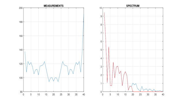
Figure 1: True spectrum $X(u)$ and the corresponding observations $J(\tau)$, $N=40$.

The precise estimates shown in Fig. 2 are obtained for this truncated spectrum zeroed for $u\geq N/2$ and shown in the upper row of the images. In the left image of this row, we show the estimates calculated for the basic interval $0\leq u\leq N/2-1.$ The perfect reconstruction is demonstrated in this case with the very small value of RMSE. In images, we show the true values and the estimates for $u\geq 1$ as the values for $u=0$ have large absolute values while RMSE are calculated for the interval $u=0,..,N/2-1$.

In the right image of the upper row, we show the estimates calculated for all $0\leq u\leq N-1$. The red color shows the true values of the spectrum, thus we can see that indeed the estimates calculated for $u\geq N/2$ are completely erroneous because the true values of the used spectra are equal to zero. There is an obvious symmetry of the estimates for $u\geq N/2$ with respect to the estimates for $u<N/2$. The right part of the estimate is obtain by mirror reflection with respect to the point $N/2+1.$

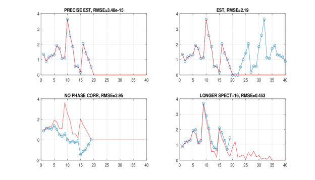
Figure 2: Spectrum reconstructions: the true values are in red and the estinates are blue with circles, $N=40.$

The second row in Fig.2 illustrates two different effects. The left estimate is calculated as it is in the first row but without the phase correction for $IFFT$ in Eq.(7). One may note that this phase correction is of importance as the estimate is completely destroyed, what can be noticed from the large values of RMSE as well as visually comparing the estimate and the true spectral values.

The last image shows the influence of the requirement $X(u)=0$ for $u\geq N/2.$ Here we assume that $X(u)=0$ for $u\geq N/2+16$. Thus, $16$ non-zero pixels of this enlarged $X(u)$ influence the $40$ observations of $J$, which are naturally different from those in Fig.1. The estimates and the corresponding true $X(u)$ are seen in Fig. 2. We may note that the estimates are destroyed with RMSE much larger than those for the perfect reconstruction demonstrated in the first row of the images.

Let us consider a set of observations $J(\tau)$ in the form

$$J(\tau)=2\sum_{u=0}^{N/2-1}X(u)(1+\cos(\frac{2\pi}{N}\tau u)),\text{ }\tau=0,1,..N-1,$$ (10)

which is different from (5) by the set of shifted $\tau$ including now $\tau=0$.

This $\tau=0$ results in significant changes in the reconstruction algorithm implemented using FFT.

Proposition 2

Let the observations $J(\tau)$, $\tau=0,1,..N-1$, be defined as in (10), then the spectra $X(u)$ can be calculated as follows:

$$X(u)=\left\{\begin{array}[c]{c}\dfrac{1}{N}\sum_{\tau=0}^{N-1}J(\tau)\cos(\frac{2\pi}{N}\tau u)\text{, if }u=1,..,N/2-1,\\ \\ \dfrac{1}{4N}\sum_{\tau=1}^{N}J(\tau)-\frac{1}{2}\sum_{u_{1}=1}^{N/2-1}X(u_{1}),\text{ if }u=0.\end{array}\right.$$ (11)

Let FFT be used for calculations of (11) and

$$x(u)=\operatorname{real}(IFFT(J(\tau))),\text{ }u\in[1,...,N],$$ (12)

then

$$X(u)=\left\{\begin{array}[c]{c}x(u+1)\text{, if }u=1,..,N/2-1,\\ \\ \dfrac{1}{4N}\sum_{\tau=0}^{N-1}J(\tau)-\frac{1}{2}\sum_{u_{1}=1}^{N/2-1}X(u_{1}),\text{ if }u=0.\end{array}\right.$$ (13)

The proofs of the formulas (11)-(13) are similar to given for the proof of Proposition 1 in Appendix.

Thus, summation on $\tau$ in (11) is produced from $\tau=0$ up to $\tau=N-1$, what is the only difference from (6). The more serious difference appeared in (12), where the phase correction specific for (7) is not required.

The solutions given by the formulas (6)-(8) and (11)-(13) are precise solutions of the equations (5) and (10) linear with respect to $X(u)$.

The properties of the estimates (11)-(13) are identical to those discussed above for solutions (6)-(8) excluding the phase correction in (7) which does not exist in (12).

Proposition 3

Let in both (5) and (10) $X(u)$ be real-valued non-negative, i.e. $X(u)=|A(u)|^{2}$, the estimates (6) and (11) continue to be valid in these cases and the estimates (8) and (13) given by FFT are simplified to the following form valid for the both estimates:

$$a(u)=abs(IFFT(J(\tau))),\text{ }u\in[1,...,N],$$ (14)

$$|A(u)|^{2}=\left\{\begin{array}[c]{c}a(u+1)\text{, if }u=1,..,N/2-1,\\ \\ \dfrac{1}{4N}\sum_{\tau=0}^{N-1}J(\tau)-\frac{1}{2}\sum_{u_{1}=1}^{N/2-1}|A(u_{1})|^{2},\text{ if }u=0.\end{array}\right.$$ (15)

The estimates (6) and (11) are valid for $X(u)=|A(u)|^{2}$ just because it is a particular case for $X(u)$. In (14) the operation $real$ is replaced by $abs$ just because $|A(u)|^{2}$ are non-negative. Then, the complex exponent in (7) is killed by $abs$ and the estimates in both Proposition 1 and Proposition 2 take the identical form presented above in Proposition 3.

Note, that $a(u)$ in (14) can be calculated using $FFT$ as

$$a(u)=abs(FFT(J(\tau)))/N,\text{ }u\in[1,...,N].$$ (16)

2.2 Symmetric sampling

Now, we consider the symmetric sampling of $J(\tau)$ with $\tau\in[-N/2,...,N/2+1]$.

Then the observation model (5) takes the form

$$J(\tau)=2\sum_{u=0}^{N/2-1}X(u)(1+\cos(\frac{2\pi}{N}\tau u)),\text{ }\tau=-N/2,..N/2-1.$$ (17)

The signal to be spectrally analyzed by observations $J(\tau)$ is of ’low band’ as it is in (5).

We say that the observations $J(\tau)$ are spectrally resolved if $X(u)$ satisfying to Eq.(17) are found.

Proposition 4

Let the observations $J(\tau)$, $\tau=-N/2,..N/2-1$, be defined according to (17), then $X(u)$ can be calculated as follows:

$$X(u)=\left\{\begin{array}[c]{c}\frac{1}{N}\sum_{\tau=-N/2}^{N/2-1}J(\tau)\cos(\frac{2\pi}{N}\tau u)\text{, if }u=1,..,N/2-1,\\ \\ \frac{1}{4N}\sum_{\tau=-N/2}^{N/2-1}J(\tau)-\frac{1}{2}\sum_{u_{1}=1}^{N/2-1}X(u_{1}),\text{ if }u=0.\end{array}\right.$$ (18)

If FFT is used for calculations these estimates can be presented in the following two forms:

(1) Let

$$x(u)=\operatorname{real}(IFFT(J(\tau))\times\exp(-j\pi(u-1))),u=1,...,N,$$ (19)

then

$$X(u)=\left\{\begin{array}[c]{c}x(u+1)\text{, }u=1,2,...,N/2-1\text{,}\\ \\ \frac{1}{4N}\sum_{\tau=-N/2}^{N/2-1}J(\tau)-\frac{1}{2}\sum_{u=1}^{N/2-1}|A(u)|^{2},\text{ if }u=0;\end{array}\right.$$ (20)

(2) Let

$$x(u)=\operatorname{real}(IFFT(fftshift(J(\tau)))),\text{ }u\in[1,...,N],$$ (21)

then

$$X(u)=\left\{\begin{array}[c]{c}x(u+1)\text{, }u=1,2,...,N/2-1\text{,}\\ \\ \frac{1}{4N}\sum_{\tau=-N/2}^{N/2-1}J(\tau)-\frac{1}{2}\sum_{u_{1}=1}^{N/2-1}X(u_{1}),\text{ if }u=0.\end{array}\right.$$ (22)

The proof of the proposition can be seen in Appendix.

Note, that the phase correction in (19) is essential as it changes signs of the items of IFFT, $\exp(-j\pi(u-1)))$ periodically takes values $1$ and $-1$, respectively for $u=1,...,N.$

This kind of the phase correction is not required for (21)-(22).

The shifts on $\Delta\tau$ of the argument in $J(\tau)$ results in the complex exponent factor for the corresponding FFT, $FFT(J(\tau+\Delta\tau))=FFT(J(\tau))\times\exp(-j\frac{2\pi}{N}\Delta\tau u)$ and $abs(FFT(J(\tau+\Delta\tau)))=abs(FFT(J(\tau)))$.

It explains, that for the problems in Propositions 1,2,3 we have identical solutions when we talk about the reconstruction of the spectrum $|A(u)|^{2}$ through FFT.

With the same reasons, the estimates (21)-(22) for $X(u)=|A(u)|^{2}$ can be replaced with

$$a(u)=abs(IFFT(\textit{fftshift}(J(\tau))))),\text{ }u=1,...,N.$$ (23)

and

$$|A(u)|^{2}=\left\{\begin{array}[c]{c}a(u+1)\text{, }u=1,2,...,N/2-1\text{,}\\ \\ \frac{1}{4N}\sum_{\tau=-N/2}^{N/2-1}J(\tau)-\frac{1}{2}\sum_{u_{1}=1}^{N/2-1}|A(u_{1})|^{2},\text{ if }u=0.\end{array}\right.$$ (24)

It is obvious, that $a(u)$ in (23) can be calculated also as

$$a(u)=abs(FFT(\textit{fftshift}(J(\tau)))))/N,\text{ }u=1,...,N.$$ (25)

2.3 Summary

1. The all estimates can be calculated as real-valued using cosine functions as it is in the initial formulations in Proposition 1- Proposition 4 with summation of the observations multiplied by $cos$ with the only difference between these estimates concerning the intervals for $\tau$, i.e. the intervals of observations.

2. The estimates for $u=0$ are always calculated accordingly to the identical formulas: see for instance the second lines in (6), (11), (18).

3. The observation models for $J(\tau)$ are linear equations with respect to $X(\omega)$ and $|A(\omega)|^{2}$ with a number of equations doubled with respect to the number of unknown. Thus, the linear algebra methods can be used in the straightforward manner.

4. The FFT as the fast conventional instrument can be considered as the preferable algorithm.  For estimation of the real valued $X(\omega)$ which can take negative values we should be careful as say in (7) FFT requires some phase correction and for the symmetric sampling fftshift should be used (21).

5. Applications for the intensity reconstruction $X(\omega)=|A(\omega)|^{2}$ are simplified as no phase corrections are required. Finally, for the all three considered cases the reconstructions are identical:

   $$a(u) =abs(IFFT(J(\tau))\text{ or }a(u)=abs(FFT(J(\tau)))/N,$$ (26)

   $$u =1,...,N,$$

   and

   $$|A(u)|^{2}=\left\{\begin{array}[c]{c}a(u+1)\text{, }u=1,2,...,N/2-1\text{,}\\ \\ \frac{1}{4N}\sum_{\tau=-N/2}^{N/2-1}J(\tau)-\frac{1}{2}\sum_{u_{1}=1}^{N/2-1}|A(u_{1})|^{2},\text{ if }u=0.\end{array}\right.$$ (27)

   The fftshift in (23) also can be omitted as it is equivalent to circular shift which is killed by $abs$.

   As it is shown in (16), (25), (26), IFFT can be replaced for FFT because $J(\tau)$ is even function of $\tau$.

3 Holography: setup with reference beam

3.1 Non-symmetric sampling

The discretization of the model (1) produced as above according to requirements of FFT, $t=\Delta_{t}\tau$ and $\omega=\Delta_{\omega}u$, where $\tau$ and $u$ are integers, results in the discrete observation model:

$$J(\tau)=\sum_{u=0}^{N/2-1}|A(u)+R\times\exp(j\frac{2\pi}{N}\tau u)|^{2},\text{ }$$

$$\sum_{u=0}^{N/2-1}(|A(u)|^{2}+|R|^{2}+RA(u)\exp(-j\frac{2\pi}{N}\tau u)+RA^{\ast}(u)\exp(j\frac{2\pi}{N}\tau u))=$$ (28)

$$\sum_{u=0}^{N/2-1}(|A(u)|^{2}+|R|^{2}+2R|A(u)|\cos(\varphi_{A}(u)-\frac{2\pi}{N}\tau u)),$$

$$\tau=1,..N,$$

where the integer discrete frequency cover the interval $u\in\{0,1,...,N/2-1\}$, as we assume that the signal $A(u)$ is low band such that $A(u)=0$ for $u\geq N/2.$

Proposition 5

Let the observations $J(\tau)$, $\tau=1,..N$ be defined as in Eq.(28), then $A(u)$ can be calculated as follows:

$$A(u) =\frac{1}{NR}\sum_{\tau=1}^{N}J(\tau)\exp(j\frac{2\pi}{N}\tau u)\text{, }0<u\leq N/2-1,$$ (29)

$$|A(0)+R|^{2} =\sum_{\tau=1}^{N}J(\tau)-(\sum_{u_{1}=1}^{N/2-1}|A(u_{1})|^{2}+\sum_{u_{1}=1}^{N/2-1}R^{2})\text{, }u=0.$$

The calculations with FFT similar to (8) are as follows:

$$a(u)=IFFT(J(\tau))\times\exp(j\frac{2\pi}{N}(u-1)),\text{ }u=1,...,N,$$ (30)

and

$$A(u) =\frac{1}{R}a(u+1)\text{, if }u=1,..,N/2-1,$$ (31)

$$|A(0)+R|^{2} =\frac{1}{N}\sum_{\tau=1}^{N}J(\tau)-(\sum_{u_{1}=1}^{N/2-1}|A(u_{1})|^{2}+\sum_{u_{1}=1}^{N/2-1}R^{2})\text{, if }u=0\text{.}$$

The phase correction in (30) is as in (8) but the operation $real$ is dropped. The proof of these formulas can be found in Appendix.

If the reference beam $R$ is known, $A(u)$ is defined in the first row of (31) for $u>0$ and $A(0)$ from the second row. There is no a unique solution for the complex-valued $A(0)$ from the second equation (31). However, if we assume that $A(0)$ is real non-negative, what is natural for the zero frequency of the object, then the unique solution is of the form

$$A(0)=\sqrt{\frac{1}{N}\sum_{\tau=1}^{N}J(\tau)-(\sum_{u_{1}=1}^{N/2-1}|A(u_{1})|^{2}+\sum_{u_{1}=1}^{N/2-1}R^{2})}-R.$$ (32)

Note, that the expression under the square root is always positive.

In what follows, we show simulation tests illustrating the derived estimates for the complex valued $A(u)$. It is assumed that $A(0)$ is real-valued non-negative.

In Fig.3 we show the measurements $J(t)$, the true amplitudes of $A$ (non-negative random values with uniform distribution) and the true phases of $A$ (random Gaussian with $\sigma=.5).$ The number of observations $N=40$. According to the above results the perfect reconstruction is guaranteed provided that $A(u)=0$ for $u\geq N/2$ and for $0\leq u\leq N/2-1$. The observations are obtained from $A$ are shown in Fig.3 by zeroing values for $u\geq N/2$. This true values of the amplitude and phase are marked by red for $0\leq u\leq N/2-1$.

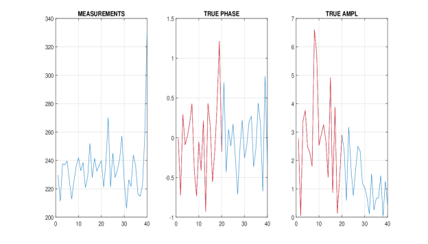
Figure 3: Measurements $J(\tau)$ and true phase and amplitude for the non-symmetric sampling.

The precise estimates shown in Figs. 4 and 5 are obtained for the truncated spectrum of the signal which takes zero values for $u\geq N/2$.

The estimates for the phase are shown in the upper row of the images in Fig. 4. In the left image of this row we show the estimates calculated for the basic interval $0\leq u\leq N/2-1.$ The perfect reconstruction is demonstrated in this case with the very small value of RMSE. In the right image, we show the estimates calculated for all $0\leq u\leq N-1$. The red color shows the true values of the signal. We can see that the estimates calculated for $u\geq N/2$ are completely erroneous very different from the true values equal to zero. The RMSE is calculated for the second part of the $\ u$ interval and it is very large.

There is an obvious symmetry of the estimates for $u\geq N/2$ with respect to the estimates for $u<N/2$. The right part of the estimate can be interpreted as the negative mirror reflection with respect to the point $N/2+1$ with the phase values taken with the sign minus.

The second row in Fig. 4 illustrates the effects of two different factors. The left estimate is calculated as it in the first row but without the phase correction  for $IFFT$ in Eq.(30). One may note that this phase correction is of importance as the estimate is completely destroyed, what can be noticed from the large values of RMSE as well as visually comparing the estimate and the true values.

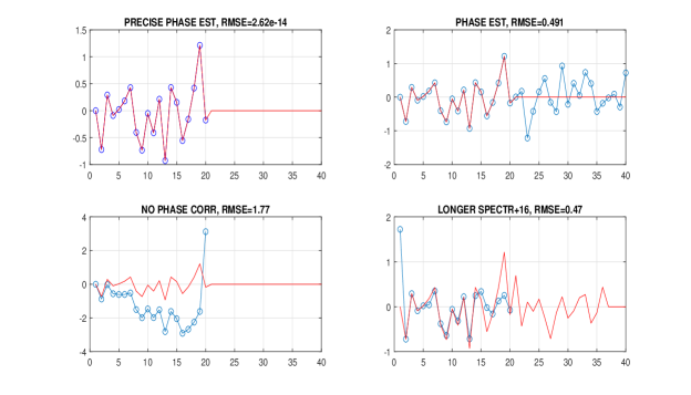
Figure 4: Phase reconstructions: non-symmetric sampling.

The last image in Fig. 4 shows the influence of the condition $A(u)=0$ for $u\geq N/2$ for the phase estimation. Here we assume that $A(u)=0$ for $u\geq N/2+16$. Thus, $16$ pixels of this enlarged $A(u)$ influence the observations $J$, which are naturally different from those in Fig.3. We may note that the phase estimates are quite sensitive to this larger length of the object spectrum $A(u)$ over the basic interval $0\leq u\leq N/2-1$, at least the corresponding RMSE takes quite high value.

The estimates for the amplitude shown in Fig. 5 are obtained for the truncated spectrum of the signal which takes zero values for $u\geq N/2$. In the left image of the upper row we show the estimates calculated for the basic interval $0\leq u\leq N/2-1.$ The perfect reconstruction is demonstrated in this case with the very small value of RMSE. In the right image, we show the estimates calculated for all $0\leq u\leq N-1$. The red color shows the true values of the signal. We can see that the estimates calculated for $u\geq N/2$ are completely erroneous and very different from the true values which are zero for this interval. The RMSE is calculated for the second part of the $u$ interval and it is very large.

There is an obvious symmetry of the estimates for $u\geq N/2$ with respect to the estimates for $u<N/2$. The right part of the estimate can be interpreted as the mirror reflection with respect to the point $N/2+1$ with values taken with the positive sign what is different with respect to the symmetry of the estimates for the phase where the negative sign is appeared in reflection.

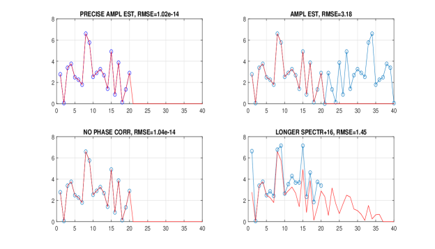
Figure 5: Amplitude reconstructions: non-symmetric sampling.

The symmetry properties of the estimates discussed here and above follow from the properties of FFT and IFFT.

The second row in Fig. 5 illustrates the effects of two different factors. The left estimate is calculated as it in the first row but without the phase correction  for $IFFT$ in Eq.(30). One may note that this phase correction naturally has no influence for the amplitude estimate.

The last image shows the influence of the non-zero values of $A(u)=0$ for $u\geq N/2.$ Here we assume that $A(u)=0$ for $u\geq N/2+16$. Thus, $16$ pixels of this enlarged $A(u)$ influence the observations $J$, which are naturally different from those in Fig.3. We may note that the amplitude estimate is quite sensitive to this extra data with RMSE taking a high value.

Similar to the case shown in Eq.(10) consider a shifted set of the observations $J(\tau)$ in the form

$$J(\tau) =\sum_{u=0}^{N/2-1}(|A(u)|^{2}+|R|^{2}+2R|A(u)|\cos(\varphi_{A}(u)-\frac{2\pi}{N}\tau u),\text{ }$$ (33)

$$\tau =0,1,..N-1,$$

which is different from (28) by the set of shifts $\tau$ including now $\tau=0$.

Proposition 6

Let the observations $J(\tau)$, $\tau=0,..N-1,$ be defined as in Eq.(33), then $A(u)$ can be calculated as follows:

$$A(u) =\frac{1}{NR}\sum_{\tau=0}^{N-1}J(\tau)\exp(j\frac{2\pi}{N}\tau u)\text{, }0<u\leq N/2-1,$$ (34)

$$|A(0)+R|^{2} =\sum_{\tau=0}^{N-1}J(\tau)-(\sum_{u_{1}=1}^{N/2-1}|A(u_{1})|^{2}+\sum_{u_{1}=1}^{N/2-1}R^{2})\text{, }u=0.$$

The calculations with FFT are similar but different from shown in (31) with

$$a(u)=IFFT(J(\tau)),\text{ }u=1,...,N,$$ (35)

then

$$A(u) =\frac{1}{R}a(u+1)\text{, if }u=1,..,N/2-1,$$ (36)

$$|A(0)+R|^{2} =\frac{1}{N}\sum_{\tau=1}^{N}J(\tau)-(\sum_{u_{1}=1}^{N/2-1}|A(u_{1})|^{2}+\sum_{u_{1}=1}^{N/2-1}R^{2})\text{, }u=0\text{.}$$

Comparing (30) with (35) we can recognize the main difference between these two estimates as the calculation of $a(u)$ for (36) does not requite the phase correction essential in (30).

We do not provide the proof of this proposition as it is similar to shown in Appendix for Proposition 5.

The numerical illustrations for this algorithm are also similar to shown in Figs. 3 - 5, naturally, without the phase correction analysis which is not required in (35).

3.2 Symmetric sampling

The measurement equations are

$$J(\tau)=\sum_{u=0}^{N/2-1}|A(u)+R\exp(j\frac{2\pi}{N}\tau u)|^{2},\text{ }$$ (37)

$$\sum_{u=0}^{N/2-1}(|A(u)|^{2}+|R|^{2}+RA(u)\exp(-j\frac{2\pi}{N}\tau u)+RA^{\ast}(u)\exp(j\frac{2\pi}{N}\tau u)),$$

$$\tau=-N/2,..N/2-1.$$

Proposition 7

Let the observations $J(\tau)$ be defined as in (37), then $A(u)$ can be calculated as follows:

$$\begin{array}[c]{c}A(u)=\frac{1}{RN}\sum_{\tau=-N/2}^{N/2-1}J(\tau)\exp(j\frac{2\pi}{N}\tau u)\text{, if }u=1,...,N/2-1,\\ \\ |A(0)+R|^{2}=\frac{1}{N}\sum_{\tau=-N/2}^{N/2-1}J(\tau)-(\sum_{u_{1}=1}^{N/2-1}|A(u_{1})|^{2}+\sum_{u_{1}=1}^{N/2-1}R^{2})\text{, }u=0.\end{array}$$ (38)

If FFT is used for calculations these estimates can be presented in the following two forms:

$$a(u)=IFFT(J(\tau))\times\exp(-j\pi(u-1)),u=1,...,N,$$ (39)

or

$$a(u)=IFFT(\textit{fftshift}(J(\tau))),\text{ }u=1,...,N,\\$$ (40)

.

then,

$$A(u) =\frac{1}{R}a(u+1)\text{, }u=1,2,...,N/2-1\text{,}$$ (41)

$$|A(0)+R|^{2} =\frac{1}{N}\sum_{\tau=-N/2}^{N/2-1}J(\tau)-(\sum_{u_{1}=1}^{N/2-1}|A(u_{1})|^{2}+\sum_{u_{1}=1}^{N/2-1}R^{2})\text{, }u=0.$$

The proof is given in Appendix.

In our simulation experiments with this latter algorithm (40)-(41) using fftshift, we assume that $A(0)$ is real positive, what allows to estimate $A(0)$ as in (32).

The observations and the true amplitude/phase images are shown in Fig.6.

Illustrations of the sensitivity of the estimates to $|A(u_{1})|^{2}>0$ for $u>N/2$ are given in Figs.7 and Figs.8 for phase and amplitude reconstructions, respectively. In the left images, the results demonstrating the perfect reconstruction are shown for the lower band spectrum and for the degradation of the reconstruction are in the right images where the spectrum is wider than $N/2$ by $16$ pixels. In the latter case visually and numerically the degradation of the estimates is essential.

The estimates in Fig.7 and Fig.8 are produced using the algorithm (39) with the phase correction for IFFT. In Fig.9 we show the results obtained by the algorithm (40) with the fftshift operation. The comparison with Fig.7 and Fig.8 confirms the identity of the results delivered by these algorithms.

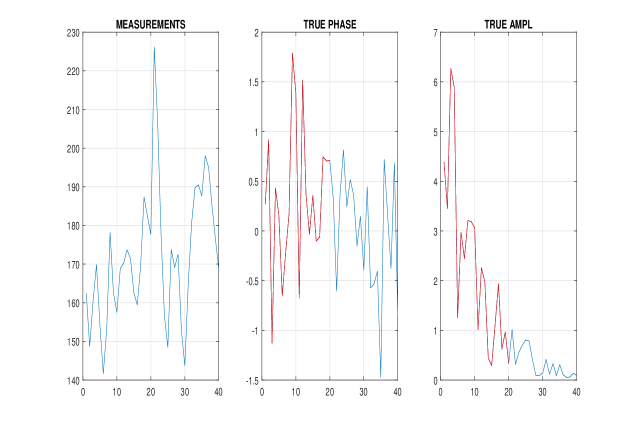
Figure 6: Observations and true  phase/amplitude for symmetric sampling.

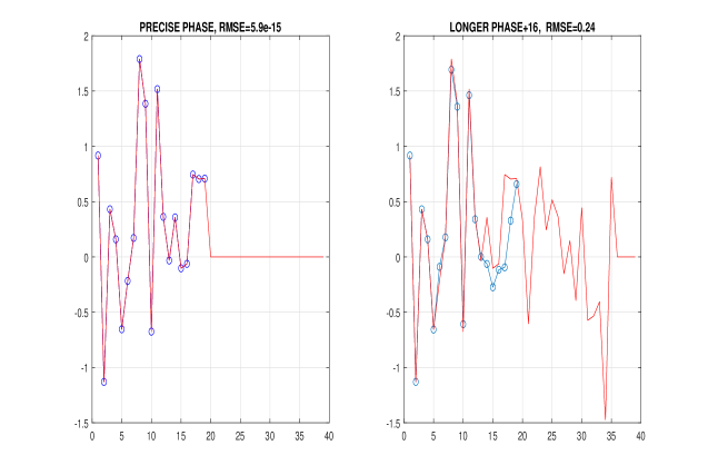
Figure 7: Phase reconstructions, effect of the longer nonzero object spectrum.

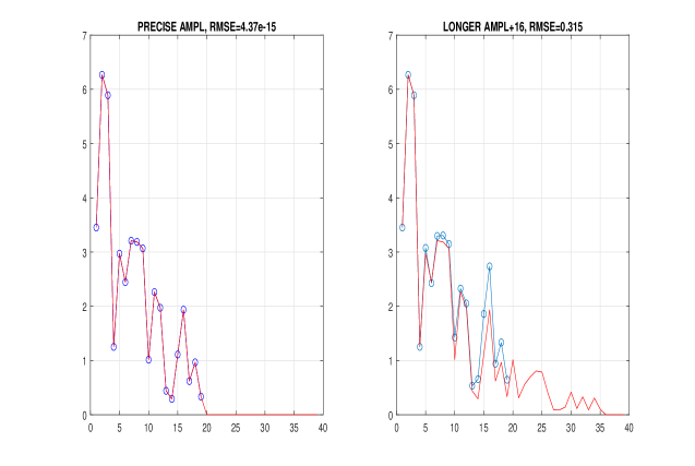
Figure 8: Amplitude reconstructions, effect of the longer nonzero object spectrum.

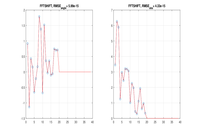
Figure 9: Perfect phase and amplitude reconstructions by IFFT with the fftshift operation.

3.3 Summary

1. The all estimates can be calculated as FFT or IFFT of the observations, see (30), (35), (40) with the summation interval defined by the observation shifts.

2. The estimates for $u=0$ are always calculated accordingly to the similar formulas: see for instance the second lines in (29), (34), (38).

3. The FFT as the fast conventional instrument can be considered as a preferable algorithm. The most compact form of estimation is achieved using fftshift together with $IFFT$ in (40).

4. The MATLAB demo-codes reproducing the presented numerical tests are publicly available: http://www.cs.tut.fi/sgn/imaging/sparse/.

4 Appendix

4.1 The proof of Proposition 1

Remind, that the Kronecker delta-function defined for integer $n,m$ as

$$\frac{1}{N}\sum_{k=1}^{N}\exp(j2\pi(n-m)k/N)=\delta_{n,m}$$ (42)

is periodic on $(n-m)$. We apply it only for the single period

$$|n-m|<N.$$ (43)

Using this definition of the Kronecker function and the expression

$$\cos(\frac{2\pi}{N}\tau u)\cos(\frac{2\pi}{N}\tau v) =\frac{1}{4}[(\exp(j\frac{2\pi}{N}\tau u)+\exp(-j\frac{2\pi}{N}\tau u))$$ (44)

$$+(\exp(j\frac{2\pi}{N}\tau v)+\exp(-j\frac{2\pi}{N}\tau v))],$$

simple calculations show that for integer $u$ and $v$

$$\frac{2}{N}\sum_{\tau=1}^{N}\cos(\frac{2\pi}{N}\tau u)\cos(\frac{2\pi}{N}\tau v)=\delta_{u,v}+\delta_{u,-v},$$ (45)

$$u,v\in[0,..,N/2-1].$$

The later restrictions on $u$ and $v$ are essential as they guarantee that $|u-v|<N$ and $|u+v|<N$ and only the single period of the Kronecker function is in use for (44).

Let us calculate $\dfrac{1}{N}\sum_{\tau=1}^{N}J(\tau)\cos(\frac{2\pi}{N}\tau u)$ inserting the expression for $J(\tau)$, Eq.(5), and using Eq.(45).

Then,

$$\frac{2}{N}\sum_{\tau=1}^{N}\sum_{u_{1}=0}^{N/2-1}X(u_{1})(1+\cos(\frac{2\pi}{N}\tau u_{1}))\cos(\frac{2\pi}{N}\tau u)=$$

$$\sum_{u_{1}=0}^{N/2-1}X(u_{1})[\frac{2}{N}\sum_{\tau=1}^{N}\cos(\frac{2\pi}{N}\tau u)+\frac{2}{N}\sum_{\tau=1}^{N}\cos(\frac{2\pi}{N}\tau u_{1})\cos(\frac{2\pi}{N}\tau u)]=$$

$$\sum_{u_{1}=0}^{N/2-1}X(u_{1})[2\delta_{u,0}+\delta_{u,u_{1}}+\delta_{u,-u_{1}}]=2\sum_{u_{1}=0}^{N/2-1}X(u_{1})\delta_{u,0}+|A(u)|^{2}+|A(0)|^{2}\delta_{u,0}.$$ (46)

Thus, we obtain that

$$\frac{1}{N}\sum_{\tau=1}^{N}J(\tau)\cos(\frac{2\pi}{N}\tau u)=2\sum_{u_{1}=0}^{N/2-1}X(u_{1})\delta_{u,0}+X(u)+X(0)\delta_{u,0}.$$ (47)

The first line of (6) follows from (47) if $u=1,..,N/2-1$. For $u=0,$ we obtain from (47)

$$\frac{1}{N}\sum_{\tau=1}^{N}J(\tau)=2\sum_{u_{1}=0}^{N/2-1}X(u_{1})+X(0)+X(0)=$$ (48)

$$4X(0)+2\sum_{u_{1}=1}^{N/2-1}X(u_{1}).$$

and the second line of (6) follows from the last formulas.

We can use for (6) the complex exponent, then

$$X(u)=\left\{\begin{array}[c]{c}\frac{1}{N}\operatorname{real}(\sum_{\tau=1}^{N}J(\tau)\exp(+j\frac{2\pi}{N}\tau u))\text{, }1\leq u\leq N/2-1,\\ \\ \frac{1}{4N}\sum_{\tau=1}^{N}J(\tau)-\frac{1}{2}\sum_{u_{1}=1}^{N/2-1}X(u_{1})\text{, }u=0,\end{array}\right.$$ (49)

then the calculations can be produced using FFT as follows

$$x(u) =\operatorname{real}(IFFT(J(\tau))\times\exp(j\frac{2\pi}{N}(u-1))),$$

$$u =1,..,N.$$

Then, the formula (49) can be rewritten as

$$X(u)=\left\{\begin{array}[c]{c}x(u+1)\text{, if }u=1,..,N/2-1,\\ \\ \dfrac{1}{4N}\sum_{\tau=1}^{N}J(\tau)-\frac{1}{2}\sum_{u_{1}=1}^{N/2-1}X(u_{1}),\text{ if }u=0.\end{array}\right.$$

what confirms (8).

It completes the proof of Proposition 1.

4.2 The proof of Proposition 4.

For the symmetric sampling observation model is of the form:

$$J(\tau)=\sum_{u=0}^{N/2-1}X(u)(2+\exp(-j\frac{2\pi}{N}\tau u)+\exp(j\frac{2\pi}{N}\tau u)),$$ (50)

$$\tau=-N/2,...,N/2-1.$$

We calculate DFT of $J(\tau)$ as follows

$$\frac{1}{N}\sum_{\tau=-N/2}^{N/2-1}J(\tau)\exp(j\frac{2\pi}{N}\tau u_{1})=$$ (51)

$$\sum_{u=0}^{N/2-1}\frac{1}{N}\sum_{\tau=-N/2}^{N/2-1}X(u)(2+\exp(-j\frac{2\pi}{N}\tau u)+\exp(j\frac{2\pi}{N}\tau u))\exp(j\frac{2\pi}{N}\tau u_{1})=$$

$$\sum_{u=0}^{N/2-1}[X(u)(2\delta_{u_{1},0}+\delta_{u,u_{1}}+\delta_{u,-u_{1}}]=$$

$$\sum_{u=0}^{N/2-1}X(u)2\delta_{u_{1},0}+X(u_{1})^{2}+X(0)\delta_{u_{1},0}.$$

It follows that

$$X(u_{1}) =\frac{1}{N}\operatorname{real}(\sum_{\tau=-N/2}^{N/2-1}J(\tau)\exp(j\frac{2\pi}{N}\tau u_{1}))\text{, }1\leq u_{1}\leq N/2-1,$$ (52)

$$X(0) =(\frac{1}{N}\sum_{\tau=-N/2}^{N/2-1}J(\tau)-2\sum_{u=1}^{N/2-1}|A(u)|^{2})/4,\text{ }u_{1}=0.$$

The last equation follows from Eq.(51) for $u_{1}=0$. It proves Eqs.(18).

In order to derive the formulas with FFT, we produce a change of the summation variable in the first line of (52):

$$\frac{1}{N}\sum_{\tau=-N/2}^{N/2-1}J(\tau)\exp(j\frac{2\pi}{N}\tau u_{1})=\frac{1}{N}\sum_{\tau_{1}=0}^{N-1}J(\tau_{1}-N/2)\exp(j\frac{2\pi}{N}(\tau_{1}-N/2)u_{1})=$$ (53)

$$\frac{1}{N}\sum_{\tau_{1}=0}^{N-1}J(\tau_{1}-N/2)\exp(j\frac{2\pi}{N}(\tau_{1}u_{1}))\exp(-j\pi u_{1})=$$

$$IFFT(J(\tau))\times\exp(-j\pi(u_{1}-1)),\text{ }1\leq u_{1}\leq N/2-1.$$

where

$$IFFT(J(\tau))=\frac{1}{N}\sum_{\tau=1}^{N}J(\tau)\exp(j\frac{2\pi}{N}(\tau-1)(u-1)).$$

The last expression in (53) proves Eq. (19).

In order to prove (21)-(22) note, that the sequence $J(\tau)$ in (18) is ordered according to $\tau\in[-N/2,-N/2+1,...,-1,0,1,...,N/2-1]$. The MATLAB fftshift operation in (21) circularly shifts $\tau=0$ to the initial position and the sequence takes the form $\tau\in[0,1,...,N/2-1,-N/2,-N/2+1,...,-1]$. The $J(\tau)$ is periodic with the period equal to $N$, $J(\tau)=J(\tau+N).$ We add $N$ to the negative items of the obtained sequence and arrive to another sequence $\tau\in[0,1,..,N-1]$ with the values of $J(\tau)$ identical to those for the initial sequence $\tau\in[-N/2,-N/2+1,...,-1,0,1,...,N/2-1]$.

In order to extract the values $X(u)$ from this sequence we use the results of Proposition 2 dealing exactly with such sequence of $J(\tau)$, $\tau\in[0,1,..,N-1]$. Then, the formulas (12)-(13) can be used for this reconstruction.

It proves Eqs. (21)-(22) and completes the proof of the proposition.

4.3 The proof of Proposition 5.

Observations are of the form

$$J(\tau)=\sum_{u=0}^{N/2-1}|A(u)+R\exp(j\frac{2\pi}{N}\tau u)|^{2},\text{ }\tau=1,..N.$$ (54)

$$\sum_{u=0}^{N/2-1}(|A(u)|^{2}+R^{2}+RA(u)\operatorname{A}\exp(-j\frac{2\pi}{N}\tau u)+RA^{\ast}(u)\exp(j\frac{2\pi}{N}\tau u)).$$

Let us calculate DFT for $J(\tau):$

$$\frac{1}{N}\sum_{\tau=1}^{N}J(\tau)\exp(j\frac{2\pi}{N}\tau u_{1})=$$

$$\sum_{u=0}^{N/2-1}\frac{1}{N}\sum_{\tau=1}^{N}[(|A(u)|^{2}+R^{2}+RA(u)\exp(-j\frac{2\pi}{N}\tau u)+$$

$$RA^{\ast}(u)\exp(j\frac{2\pi}{N}\tau u))]\exp(j\frac{2\pi}{N}\tau u_{1})=$$

$$\sum_{u=0}^{N/2-1}[(|A(u)|^{2}\delta_{u_{1},0}+R^{2}\delta_{u_{1},0}+RA(u)\delta_{u,u_{1}}+RA^{\ast}(u)\delta_{u,-u_{1}}]=$$

$$\sum_{u=0}^{N/2-1}|A(u)|^{2}\delta_{u_{1},0}+\sum_{u=0}^{N/2-1}R^{2}\delta_{u_{1},0}+RA(u_{1})+RA^{\ast}(0)\delta_{u_{1},0}].$$

Here we use the definition of the Kronecker $\delta$-function (42). It results in

$$RA(u_{1}) =\frac{1}{N}\sum_{\tau=1}^{N}J(\tau)\exp(j\frac{2\pi}{N}\tau u_{1})\text{, }1\leq u_{1}\leq N/2-1,$$ (55)

$$|A(0)+R(0)|^{2} =\frac{1}{N}\sum_{\tau=1}^{N}J(\tau)-(\sum_{u=1}^{N/2-1}|A(u)|^{2}+\sum_{u=1}^{N/2-1}R^{2}),\text{ }u_{1}=0.$$

Using $IFFT$ we arrive to the formula

$$A(u) =\frac{1}{R}IFFT(J(\tau))\exp(j\frac{2\pi}{N}\tau(u-1))\text{, }1\leq u\leq N/2-1,$$

$$|A(0)+R(0)|^{2} =\frac{1}{N}\sum_{\tau=1}^{N}J(\tau)-(\sum_{u_{1}=1}^{N/2-1}|A(u_{1})|^{2}+\sum_{u_{1}=1}^{N/2-1}R^{2})\text{, }u=0,$$

what can be written in the form (31).

It completed the proof of Proposition 5.

4.4 The proof of Proposition 7

Observations are of the form:

$$J(\tau)=\sum_{u=0}^{N/2-1}|A(u)+R\cdot\exp(j\frac{2\pi}{N}\tau u)|^{2},\text{ }\tau=-N/2,..,N/2-1.$$

$$\sum_{u=0}^{N/2-1}(|A(u)|^{2}+R^{2}+RA(u)\exp(-j\frac{2\pi}{N}\tau u)+RA^{\ast}(u)\exp(j\frac{2\pi}{N}\tau u)).$$

Calculate DFT for these observations

$$\frac{1}{N}\sum_{\tau=-N/2}^{N/2-1}J(\tau)\exp(j\frac{2\pi}{N}\tau u_{1})=$$ (56)

$$\sum_{u=0}^{N/2-1}\frac{1}{N}\sum_{\tau=-N/2}^{N/2-1}[(|A(u)|^{2}+R^{2}+RA(u)\exp(-j\frac{2\pi}{N}\tau u)+$$

$$RA^{\ast}(u)\exp(j\frac{2\pi}{N}\tau u))]\exp(j\frac{2\pi}{N}\tau u_{1})=$$

$$\sum_{u=0}^{N/2-1}[(|A(u)|^{2}\delta_{u_{1},0}+R^{2}\delta_{u_{1},0}+RA(u)\delta_{u,u_{1}}+RA^{\ast}(u)\delta_{u,-u_{1}}]=$$

$$\sum_{u=0}^{N/2-1}|A(u)|^{2}\delta_{u_{1},0}+\sum_{u=0}^{N/2-1}R^{2}\delta_{u_{1},0}+RA(u_{1})+RA^{\ast}(0)\delta_{u_{1},0}].$$

The results are as follows

$$RA(u) =\frac{1}{N}\sum_{\tau=-N/2}^{N/2-1}J(\tau)\exp(j\frac{2\pi}{N}\tau u)\text{, }1\leq u\leq N/2-1,$$ (57)

$$|A(0)+R(0)|^{2} =\frac{1}{N}\sum_{\tau=-N/2}^{N/2-1}J(\tau)-(\sum_{u_{1}=1}^{N/2-1}|A(u_{1})|^{2}+\sum_{u_{1}=1}^{N/2-1}R^{2}),\text{ }u=0.$$

It proves (38).

Let us produce the transformations in the first line equation in Eq.(57) similar to used in the proof of Proposition 4: $\frac{1}{N}\sum_{\tau=-N/2}^{N/2-1}J(\tau)\exp(j\frac{2\pi}{N}\tau u_{1})=\frac{1}{N}\sum_{\tau_{1}=0}^{N-1}J(\tau_{1}-N/2)\exp(j\frac{2\pi}{N}(\tau_{1}u_{1}))\exp(-j\pi u_{1})$ and introduce

$$a(u)=IFFT(J(\tau))\times\exp(-j\pi(u-1)),u\in[1,...,N],$$ (58)

then Eq.(57) takes the form:

$$A(u) =\frac{1}{R}a(u+1)\text{, }u=1,2,...,N/2-1\text{,}$$ (59)

$$|A(0)+R|^{2} =\frac{1}{N}\sum_{\tau=-N/2}^{N/2-1}J(\tau)-(\sum_{u_{1}=1}^{N/2-1}|A(u_{1})|^{2}+\sum_{u_{1}=1}^{N/2-1}R^{2})\text{, }u=0.$$

It proves the algorithm with $a(u)$ defined as in (39).

The phase correction by the complex exponent $\exp(-j\pi(u-1))$ is essential for this form of the solution.

In order to simplify this solution, we involve fftshift operation as it is in the proof of Proposition 4 and arrive to the following compact expression:

$$a(u)=IFFT(\textit{fftshift}(J(\tau))),u\in[1,...,N],$$ (60)

then

$$A(u) =\frac{1}{R}a(u+1)\text{, }u=1,2,...,N/2-1\text{,}$$ (61)

$$|A(0)+R|^{2} =\frac{1}{N}\sum_{\tau=-N/2}^{N/2-1}J(\tau)-(\sum_{u_{1}=1}^{N/2-1}|A(u_{1})|^{2}+\sum_{u_{1}=1}^{N/2-1}R^{2})\text{, }u=0.$$

It confirms Eqs.(40)-(41) and completes the proof of Proposition 7.

5 ACKNOWLEDGMENTS

This work is done as a part of CIWIL project funded by Jane and Aatos Erkko Foundation and supported by Finnish Academy of Science, Project No. 287150, 2015-2019.

References

- [1] U. Schnars and W. Juptner, Digital Holography: Digital Hologram Recording, Numerical Reconstruction, and Related Techniques (Springer Berlin Heidelberg, 2005).
- [2] M. K. Kim, “Principles and techniques of digital holographic microscopy,” SPIE Rev. 1(1), 1–50 (2010).
- [3] Kalenkov, G. S. Kalenkov, and A. E. Shtanko, “The Fourier-spectrometer as a holographic micro-object imaging system in low-coherence light,” Meas. Tech. 55(11), 21–25 (2012).
- [4] G. Kalenkov, G. S. Kalenkov, and A. E. Shtanko, ”Hyperspectral holography: an alternative application of the Fourier transform spectrometer,” JOSA B, 34(5): B49, 2017.
- [5] R. J. Bell, Introductory Fourier Transform Spectroscopy (Academic Pr., 1972, New York).
- [6] Sumner P. Davis, Mark C. Abrams, James W. Brault, ”Fourier Transform Spectrometry,” Academic Press, 2001, Science 262 pp.
- [7] C. Falldorf, R. Klattenhoff and R. B. Bergmann, ”Single shot lateral shear interferometer with variable shear,” Optical Engineering 54(5), 054105, 2015.