The Effects of the Problem Hamiltonian Parameters on the Minimum Spectral Gap in Adiabatic Quantum Optimization

Abstract

We study the relation between the Ising problem Hamiltonian parameters and the minimum spectral gap (min-gap) of the system Hamiltonian in the Ising-based quantum annealer. The main argument we use in this paper to assess the performance of a QA algorithm is the presence or absence of an anti-crossing during quantum evolution. For this purpose, we introduce a new parametrization definition of the anti-crossing. Using the Maximum-weighted Independent Set (MIS) problem in which there are flexible parameters (energy penalties $J$ between pairs of edges) in an Ising formulation as the model problem, we construct examples to show that by changing the value of $J$, we can change the quantum evolution from one that has an anti-crossing (that results in an exponential small min-gap) to one that does not have, or the other way around, and thus drastically change (increase or decrease) the min-gap. However, we also show that by changing the value of $J$ alone, one can not avoid the anti-crossing. We recall a polynomial reduction from an Ising problem to an MIS problem to show that the flexibility of changing parameters without changing the problem to be solved can be applied to any Ising problem. As an example, we show that by such a reduction alone, it is possible to remove the anti-crossing and thus increase the min-gap. Our anti-crossing definition is necessarily scaling invariant as scaling the problem Hamiltonian does not change the nature (i.e. presence or absence) of an anti-crossing. As a side note, we show exactly how the min-gap is scaled if we scale the problem Hamiltonian by a constant factor.

1 Introduction

In this paper, we seek to understand the quantum evolution of the adiabatic quantum optimization algorithm (see e.g. [2] for a recent review) by studying how different parameters of the Ising problem Hamiltonian affect the minimum spectral gap (min-gap) of the system Hamiltonian in the Ising-based quantum annealer (QA). We consider the standard quantum annealing protocol with the following system Hamiltonian:

$${\mathcal{H}}(s)=(1-s){\mathcal{H}}_{\mathsf{driver}}+s{\mathcal{H}}_{\mathsf{Ising}}$$ (1)

where ${\mathcal{H}}_{\mathsf{driver}}=-\sum_{i\in{\mathsf{V}}(G)}\sigma^{x}_{i}$ is the standard transverse field Hamiltonian unless otherwise specified, and ${\mathcal{H}}_{\mathsf{Ising}}=\sum_{i\in{\mathsf{V}}(G)}h_{i}\sigma^{z}_{i}+\sum_{ij\in{\mathsf{E}}(G)}J_{ij}\sigma^{z}_{i}\sigma^{z}_{j}$ is an Ising Hamiltonian defined on a graph $G=({\mathsf{V}}(G),{\mathsf{E}}(G))$.

We use the Maximum-weighted Independent Set (MIS) as the model problem for our investigation as it admits a natural parameter-flexible Ising Hamiltonian formulation, referred to as the MIS-Ising Hamiltonian (to be defined in Section 3.1). That is, we can change parameters ($h,J$) of the MIS-Ising Hamiltonian without changing the problem to be solved. Moreover, any Ising Hamiltonian can be easily and efficiently expressed as an MIS-Ising Hamiltonian because any Ising problem can be so reduced to an MIS problem (a reduction procedure is described in Section 3.2).

The main argument we use in this paper to assess the performance of a QA algorithm is the presence or absence of an anti-crossing during quantum evolution. For this purpose, we introduce a new parametrization definition for the anti-crossing (to be described in Section 2). The question we ask is then: what are the factors of a QA algorithm that contribute to the presence or absence of an anti-crossing that results in an exponentially small min-gap (which determines the running time of the algorithm)?

In this paper, we propose a preliminary answer for this question, when the initial ground state is the uniform superposition state (i.e. $\frac{1}{\sqrt{2^{n}}}\sum_{i=0}^{2^{n}-1}|i\rangle$, as in the case of the transverse-field drive Hamiltonian): the presence or absence of an anti-crossing depends on the relation of the ground state and the first excited state (of the problem Hamiltonian) with their low-energy (driver Hamiltonian dependent) neighboring states (LENS). Roughly speaking, with the uniform superposition state as the initial ground state, if the ground state has more LENS than the first excited state does, there is no anti-crossing and the min-gap is large, but if the first excited state has more LENS than the ground state does, there is an anti-crossing resulting in a small min-gap. The factors that affect the LENS include the type of driver Hamiltonian ($X$-driver: ${\mathcal{H}}_{X}=-\sum_{i\in{\mathsf{V}}(G)}\sigma_{i}^{x}$; or $XX$-driver: ${\mathcal{H}}_{XX}^{\lambda}=-\sum_{i\in{\mathsf{V}}(G)}\sigma_{i}^{x}+\lambda\sum_{ij\in{\mathsf{E}}(G_{\mathsf{driver}})}\sigma_{i}^{x}\sigma_{j}^{x}$, where $\lambda$ can be a positive or negative number), the driver graph $G_{\mathsf{driver}}$ (in the $XX$-driver case), and the energy spectrum of states (of the problem Hamiltonian). In this paper, we consider mainly $X$-driver Hamiltonian. The case of $XX$-driver Hamiltonian, both stoquastic and non-stoquastic, and different driver graphs are studied in [9]. Based on our LENS observation, we construct examples to answer the questions we study, namely, how different parameters can or can not change the min-gap by the presence or absence of an anti-crossing.

The paper is organized as follows. In Section 2, we introduce a new parametrization definition for the anti-crossing. We revisit in Section 3 the NP-hard Maximum-weighted Independent Set (MIS) problem. In Section 3.1 we rederive the parameter-flexible MIS-Ising Hamiltonian. We recall an efficient reduction to convert an Ising problem to an MIS problem in Section 3.2. As a side example, we apply the Ising-MIS reduction on the loop gadgets, the Ising instances that were constructed by Tameem Albash to have small min-gaps to show the evidence of quantum tunneling. We show that the resulting MIS-Ising Hamiltonians no longer have an anti-crossing (even without the need to change the parameters) and the min-gaps are large. In Section 4, we describe our LENS idea. Then we construct two examples based on the idea. In Section 4.1, we construct Example 1 to show that one can change the parameter $J$ (without changing the problem to be solved) to change the quantum evolution (from the presence of an anti-crossing to the absence of one, or vice versa). In Section 4.2, we construct Example 2 to show that by changing the value of $J$ alone, one can not avoid the anti-crossing. In Section 5, we show exactly how the min-gap is scaled if we scale the problem Hamiltonian by a constant factor. Thus there is no need for renormalization of the parameters in order for the comparison of different parameter QA algorithms, as we know exactly how much the contribution is due to the scaling, and how much is due to the different value of the parameter. We conclude with a discussion in Section 6.

2 A Parametrization Definition of An Anti-crossing

Anti-crossing, also known as avoided level crossing or level repulsion, is a well-known concept for physicists. A parametrized definition of an anti-crossing is given by Wilkinson in [19, 20]. In this definition, the energy levels in the neighborhood of an anti-crossing at $s^{*}$ takes the form of a hyperbola:

$$E^{\pm}(s)=E(s^{*})+B(s-s^{*})\pm\frac{1}{2}[\Delta_{min}^{2}+A^{2}(s-s^{*})^{2}]^{1/2}$$ (2)

where $\Delta_{min}$ denote the min-gap size, $A$ and $B$ are respectively the difference and the mean of the slopes of the asymptotes of the hyperbola (referred as the asymptotic slopes of the two curves in the original paper).

For example, such a definition was adopted in a recent paper [17] to study the effect of noise on the quantum system. The derivation of the formula is based on the idea that in the neighborhood of $s^{*}$ the behavior of these two energy levels can be described by degenerate perturbation theory: the energy levels are eigenvalues of the $2\times 2$ matrix

$$H=\begin{bmatrix}e^{+}&h\\ h&e^{-}\end{bmatrix}.$$

However, for our purpose (to identify an anti-crossing based on the numerical diagonization of the Hamiltonian), we introduce the following parametrization. This parametrization is also based on the same idea that in the neighborhood of $s^{*}$ the behavior of these two energy levels can be described by degenerate perturbation theory. But instead of the energy values alone, we make use of the two strongly mixed eigenstates to identify the avoided crossing point. It is likely that the similar but probably non-quantitative idea has been described somewhere in the literature.

Let $|E_{k}(s)\rangle$ ($E_{k}(s)$ respectively) be the instantaneous eigenstate (energy respectively) of the system Hamiltonian ${\mathcal{H}}(s)$ in Eq.(1) at time $s$, i.e.,

$${\mathcal{H}}(s)|E_{k}(s)\rangle=E_{k}(s)|E_{k}(s)\rangle$$

for $k=0,1,\ldots.$ We order and represent the states so that the energies are strictly increasing as the index increases:

$$E_{0}(s)<E_{1}(s)<E_{2}(s)<\ldots$$

That is, if there are some degenerate states, we represent the corresponding state as a superposition of the degenerate states. We will focus on the lowest two instantaneous eigenstates, namely, $|E_{0}(s)\rangle$, the instantaneous ground state, and $|E_{1}(s)\rangle$, the instantaneous first excited state. In particular, ${\mathsf{mingap}}=\min_{s\in[0,1)}E_{1}(s)-E_{0}(s)=E_{1}(s^{*})-E_{0}(s^{*})$, where $s^{*}$ is the min-gap position. We are interested in whether there is an anti-crossing occurrence at $s^{*}$.

When $s=1$, the states$|E_{k}(1)\rangle$ and energies $E_{k}(1)$ are of the problem (final) Hamiltonian. Again, we mainly focus on the lowest two levels for $k=0$ and $k=1$. For convenience, we denote $|\mathsf{GS}\rangle\stackrel{{\scriptstyle\mathrm{def}}}{{=}}|E_{0}(1)\rangle$, the ground state (encode solution, possibly degenerate) of the problem Hamiltonian, and $|\mathsf{FS}\rangle\stackrel{{\scriptstyle\mathrm{def}}}{{=}}|E_{1}(1)\rangle$, the superposition of the possibly degenerate first excited states. We will express the instantaneous eigenstates ($|E_{0}(s)\rangle,|E_{1}(s)\rangle$) in terms of the eigenstates ($|E_{k}(1)\rangle$) of the final Hamiltonian.

Define

$$a_{k}(s)=|\langle E_{k}(1)|{E_{0}(s)}\rangle|^{2}$$ (3)

$$b_{k}(s)=|\langle E_{k}(1)|{E_{1}(s)}\rangle|^{2}$$ (4)

for $k=0,1$. That is, $a_{0}(s)=|\langle\mathsf{GS}|{E_{0}(s)}\rangle|^{2}$ is the weight (or overlap) of the solution state with the instantaneous ground state at time $s$. Similarly, $a_{1}(s)=|\langle\mathsf{FS}|{E_{0}(s)}\rangle|^{2}$ is the weight (or overlap) of the first excited state (which possibly corresponds to the local minima of the problem) with the instantaneous ground state at time $s$. At $s=1$, we have $a_{0}(1)=b_{1}(1)=1$ and $a_{1}(1)=b_{0}(1)=0$. The evolution of $a_{k}(s)$ and $b_{k}(s)$ will play important roles to help us understand the working of the QA algorithm. In particular, we will define the anti-crossing based on the four quantities $a_{k}(s)$ and $b_{k}(s)$ for $k=0,1$.

We now introduce the definition for an anti-crossing, based on two parameters: $\gamma\geq 0$ and $\epsilon\geq 0$.

Definition.

For $\gamma\geq 0$, $\epsilon\geq 0$ we say there is an $(\gamma,\epsilon)$-Anti-crossing if there exists a $\delta>0$ such that

1. For $s\in[s^{*}-\delta,s^{*}+\delta]$,

   $$|E_{0}(s)\rangle=\sqrt{a_{0}(s)}|\mathsf{GS}\rangle+\sqrt{a_{1}(s)}|\mathsf{FS}\rangle$$ (5)

   $$|E_{1}(s)\rangle=\sqrt{b_{0}(s)}|\mathsf{GS}\rangle-\sqrt{b_{1}(s)}|\mathsf{FS}\rangle$$ (6)

   where $a_{0}(s)+a_{1}(s)\in[1-\gamma,1]$, $b_{0}(s)+b_{1}(s)\in[1-\gamma,1]$. Within the time interval $[s^{*}-\delta,s^{*}+\delta]$, both $|E_{0}(s)\rangle$ and $|E_{1}(s)\rangle$ are mainly composed of $|\mathsf{GS}\rangle$ and $|\mathsf{FS}\rangle$. That is, all other states (eigenstates of the problem Hamiltonian) are negligible (which sums up to at most $\gamma\geq 0$).

2. At the avoided crossing point $s=s^{*}$, $a_{0},a_{1},b_{0},b_{2}\in[1/2-\epsilon,1/2+\epsilon]$, for a small $\epsilon>0$. That is, $|E_{0}(s^{*})\rangle\approx 1/\sqrt{2}(|\mathsf{GS}\rangle+|\mathsf{FS}\rangle)$ and $|E_{1}(s^{*})\rangle\approx 1/\sqrt{2}(|\mathsf{GS}\rangle-|\mathsf{FS}\rangle)$.

3. Within the time interval $[s^{*}-\delta,s^{*}+\delta]$, $a_{0}(s)$ increases from $\leq\gamma$ to $\geq(1-\gamma)$, while $a_{1}(s)$ decreases from $\geq(1-\gamma)$ to $\leq\gamma$. The reverse is true for $b_{0}(s),b_{1}(s)$.

$$\begin{array}[h]{ccc}\includegraphics[width=190.79385pt]{Anticrossing4.jpg}&\includegraphics[width=78.04842pt]{AC-a01-2.jpg}&\includegraphics[width=78.04842pt]{AC-b01-2.jpg}\\ (a)&(b)&(c)\end{array}$$

Figure 1: (a) An $(\gamma,\epsilon)$-Anti-crossing. At the avoided crossing point $s=s^{*}$, $a_{0},a_{1},b_{0},b_{2}\in[1/2-\epsilon,1/2+\epsilon]$, for a small $\epsilon>0$. That is, $|E_{0}(s^{*})\rangle\approx 1/\sqrt{2}(|\mathsf{GS}\rangle+|\mathsf{FS}\rangle)$ and $|E_{1}(s^{*})\rangle\approx 1/\sqrt{2}(|\mathsf{GS}\rangle-|\mathsf{FS}\rangle)$. There exists a $\delta>0$, such that fo $s\in[s^{*}-\delta,s^{*}+\delta]$: $a_{0}(s)+a_{1}(s)\in[1-\gamma,1]$, $b_{0}(s)+b_{1}(s)\in[1-\gamma,1]$. (b) Within the time interval $[s^{*}-\delta,s^{*}+\delta]$, $a_{0}(s)$ (in red) increases, while $a_{1}(s)$ (in orange) decreases. (c) The reverse is true for $b_{0}(s)$ (in blue), and $b_{1}(s)$ (in cyan).

A figure depicting an $(\gamma,\epsilon)$-Anti-crossing is shown in Figure 1.

Remarks.

• At the avoided level crossing point $s^{*}$, the effective Hamiltonian mimics the perturbed degenerate Hamiltonian:

  $$\begin{bmatrix}1&-\lambda\\ -\lambda&1\end{bmatrix}$$

  with $|\mathsf{GS}\rangle=1/\sqrt{2}(|0\rangle+|1\rangle)$ with eigenenergy $1-\lambda$, and $|\mathsf{FS}\rangle=1/\sqrt{2}(|0\rangle-|1\rangle)$ with eigenenergy $1+\lambda$.

Parameters and Weak Anti-crossing.

The parameter $\epsilon$ is the tolerance we allow at the avoided crossing point. This parameter needs to be strict and thus we require $\epsilon$ to be very small (e.g. $\leq 0.001$). The parameter $\gamma$ corresponds to the allowed negligible states. Our numerical examples show that it is possible that the condition (2) is satisfied when $\epsilon\approx 0$, and $a_{0}(s)+a_{1}(s)$ is almost $1$ for $s\in[s^{*},s^{*}+\delta]$, but $a_{0}(s)+a_{1}(s)$ is much less than $1-\gamma$ for $s\in[s^{*}-\delta,s^{*}]$. Our numerical examples also show that when such a situation occurs, the min-gap does not occur at the exact position of $s^{*}$. For this reason, we relax the definition and refer such a case as a weak anti-crossing with one additional parameter, $\gamma^{\prime}$, where $\gamma^{\prime}>\gamma$ is the relaxed parameter such that $a_{0}(s)+a_{1}(s)>1-\gamma^{\prime}$ for $s\in[s^{*}-\delta,s^{*}]$. Notice that we maintain the strict requirement at the avoided crossing point. For the weak anti-crossing, before the avoided-crossing point, there are non-negligible states other than $|\mathsf{GS}\rangle$ and $|\mathsf{FS}\rangle$. But at the avoided crossing and after avoided crossing, the states are mainly composed of $|\mathsf{GS}\rangle$ and $|\mathsf{FS}\rangle$.

Anti-crossing and Scaling.

An anti-crossing is necessarily scaling invariant, as scaling the problem Hamiltonian should not change the nature (i.e. the presence or absence) of an anti-crossing. We discuss more on this in Section 5.

Anti-crossing vs Quantum Tunneling.

Quantum tunneling is closely related to the anti-crossing. Indeed, one feature that characterizes the presence of tunneling is by “a sharp change in the ground state of the adiabatic evolution at the degeneracy point ”[16]. This sharp change is quantified by the expectation value of the Hamming weight operator $\langle HW\rangle$ introduced there, which is readily given by $a_{1}(s)||\mathsf{FS}-\mathsf{GS}||$, where $||\mathsf{FS}-\mathsf{GS}||$ is the Hamming distance between $\mathsf{FS}$ and $\mathsf{GS}$, in our anti-crossing definition. Note that quantum tunneling is more generally described in terms of a double-well semiclassical potential, see more discussion in [16].

Anti-crossing vs Perturbative Crossing.

Our definition of anti-crossing is more general than the perturbative crossing in [4, 10]. More specifically, the perturbative crossing is defined and limited to the location near the end of evolution when the perturbation theory is applied to the problem Hamiltonian as the unperturbed Hamiltonian; whereas our anti-crossing can happen anywhere (the perturbation theory is still applicable but the unperturbed Hamiltonian is no longer the pure problem Hamiltonian). A perturbative crossing is necessarily an anti-crossing, while an anti-crossing defined here is not necessarily a perturbative crossing.

Anti-crossing and Min-gap Size.

The min-gap size is expected to be exponentially small in $O(b^{k})$ where $k=||\mathsf{FS}-\mathsf{GS}||$ for some $0<b<1$. A min-gap estimation formula for the perturbative crossing was given in [4]. It is desirable to rigorously derive a bound for the min-gap based on our more general anti-crossing definition.

Generalized Anti-crossing.

One can also generalize the defintion of the anti-crossing by replacing the first excited state $|\mathsf{FS}\rangle$ by a superposition of some neighboring low lying states. Such an example can be found in [9].

3 Maximum-Weight Independent Set (MIS) Problem

The Maximum-Weight Independent Set (MIS) problem (optimization version) is defined as:

Input: An undirected graph $G(=({\mathsf{V}}(G),{\mathsf{E}}(G)))$, where each vertex $i\in{\mathsf{V}}(G)=\{1,\ldots,n\}$ is weighted by a positive rational number $w_{i}$

Output: A subset $S\subseteq{\mathsf{V}}(G)$ such that $S$ is independent (i.e., for each $i,j\in S$, $i\neq j$, $ij\not\in{\mathsf{E}}(G)$) and the total weight of $S$ ($=\sum_{i\in S}w_{i}$) is maximized. Denote the optimal set by $\mathsf{mis}(G)$.

We recall a quadratic binary optimization formulation (QUBO) of the problem. More details can be found in [8].

Theorem 3.1 (Theorem 5.1 in [8]).

If $\lambda_{ij}\geq\min\{w_{i},w_{j}\}$ for all $ij\in{\mathsf{E}}(G)$, then the maximum value of

$${\mathcal{Y}}(x_{1},\ldots,x_{n})=\sum_{i\in{\mathsf{V}}(G)}w_{i}x_{i}-\sum_{ij\in{\mathsf{E}}(G)}\lambda_{ij}x_{i}x_{j}$$ (7)

is the total weight of the MIS. In particular if $\lambda_{ij}>\min\{w_{i},w_{j}\}$ for all $ij\in{\mathsf{E}}(G)$, then $\mathsf{mis}(G)=\{i\in{\mathsf{V}}(G):x^{*}_{i}=1\}$, where $(x^{*}_{1},\ldots,x^{*}_{n})=\operatornamewithlimits{arg\ max}_{(x_{1},\ldots,x_{n})\in\{0,1\}^{n}}{\mathcal{Y}}(x_{1},\ldots,x_{n})$.

Here the function ${\mathcal{Y}}$ is called the pseudo-boolean function for MIS, where the boolean variable $x_{i}\in\{0,1\}$, for $i=1,\ldots,n$. The proof is quite intuitive in the way that one can think of $\lambda_{ij}$ as the energy penalty when there is an edge $ij\in{\mathsf{E}}(G)$. In this formulation, we only require $\lambda_{ij}>\min\{w_{i},w_{j}\}$, and thus there is freedom in choosing this parameter.

3.1 MIS-Ising Hamiltonian

By changing the variables ($x_{i}=\frac{1+s_{i}}{2}$ where $x_{i}\in\{0,1\},s_{i}\in\{-1,1\})$, it is easy to show that MIS is equivalent to minimizing the following function, known as the Ising energy function:

$${\mathcal{E}}(s_{1},\ldots,s_{n}) = \sum_{i\in{\mathsf{V}}(G)}h_{i}s_{i}+\sum_{ij\in{\mathsf{E}}(G)}J_{ij}s_{i}s_{j},$$ (8)

which is the eigenfunction of the following Ising Hamiltonian:

$${\mathcal{H}}_{\mathsf{Ising}}=\sum_{i\in{\mathsf{V}}(G)}h_{i}\sigma^{z}_{i}+\sum_{ij\in{\mathsf{E}}(G)}J_{ij}\sigma^{z}_{i}\sigma^{z}_{j}$$ (9)

where $h_{i}=\sum_{j\in{\mathsf{nbr}}(i)}\lambda_{ij}-2w_{i}$, (conversely $w_{i}=1/2(\sum_{j\in{\mathsf{nbr}}(i)}J_{ij}-h_{i})$), $J_{ij}=\lambda_{ij}$, ${\mathsf{nbr}}(i)=\{j:ij\in{\mathsf{E}}(G)\}$, for $i\in{\mathsf{V}}(G)$.

Therefore, different $\lambda_{ij}$ in ${\mathcal{Y}}$ will correspond to different $h_{i},J_{ij}$ in ${\mathcal{H}}$ (notice that $h_{i}$ is expressed in terms of $J_{ij}$). For convenience, we will refer to a Hamiltonian in such a form as an MIS-Ising Hamiltonian. A natural question to ask is: is larger $J_{ij}$ ($=\lambda_{ij}$) better (in terms of the min-gap)? or is smaller $J_{ij}$ better? Intuitively, larger $J$ penalizes the dependent sets. However, small $J$ allows low-energy dependent sets, which can be good if they are neighbors to the ground state as we investigate and explain in the sections below.

3.2 Reduction from the Ising problem to MIS: Ising $\Longrightarrow$ MIS

In this section, we recall a polynomial reduction to convert an Ising problem to an MIS problem described in [5]. Thus, any Ising Hamiltonian can always be reduced to a parameter-flexible MIS-Ising Hamiltonian. The reduction is quite straightforward. The size of the reduced problem graph is at most $O(n+m)$ of the original graph where $n$ is the number of vertices and $m$ is the number of the edges.

The reduction consists of the following 3 steps.

Step 1: We change the variables from the spin $s_{i}\in\{-1,+1\}$ to the boolean variable $x_{i}\in\{0,1\}$, that is, from the Ising energy to a pseudo-boolean function (QUBO).

Step 2: We represent the QUBO in a posiform. The binary variable $x_{i}$ and its complement $\overline{x_{i}}=1-x_{i}$ are called together literals. Let $L=\{x_{1},\overline{x_{1}},\ldots,x_{n},\overline{x_{n}}\}$ denote the set of literals. A posiform of a pseudo-boolean function is a polynomial expression in terms of all literals such that the coefficients are all positive:

$$\phi(x_{1},\ldots,x_{n})=\sum_{T\subset L}a_{T}\prod_{u\in T}u$$

where $a_{T}>0$, $T$ is non-empty and also it does not contain $\{u,\overline{u}\}$ (otherwise the product will be zero).

Example.

Suppose ${\mathcal{Y}}(x_{1},x_{2},x_{3},x_{4})=-5.5x_{1}-3x_{2}-3x_{3}+4x_{1}x_{2}+4x_{1}x_{3}+2x_{2}x_{4}+2x_{3}x_{4}$ is the pseudo-boolean function. One possible posiform of ${\mathcal{Y}}$ can be $\phi(x_{1},x_{2},x_{3},x_{4})=-11.5+5.5\overline{x_{1}}+3\overline{x_{2}}+3\overline{x_{3}}+4x_{1}x_{2}+4x_{1}x_{3}+2x_{2}x_{4}+2x_{3}x_{4}$, by replacing $-x_{i}$ with $(\overline{x_{i}}-1)$.

Step 3: Given a posiform, we then associate to it a weighted graph $G_{\phi}$, called its conflict graph. Vertices of $G_{\phi}$ correspond to the nontrivial terms of $\phi$, i.e. ${\mathcal{T}}=\{T\subset L:T\neq\emptyset,a_{T}>0\}.$ To a vertex $T\in{\mathcal{T}}$ we associate $a_{T}$ as its weight. Two terms $T,T^{\prime}$ are in conflict if there is a literal $u\in T$ for which $\overline{u}\in T^{\prime}$. The edges of $G_{\phi}$ correspond to the conflicting pairs of terms. Since there are $O(n+m)$ terms in the posiform, where $n,m$ are the number of vertices and edges of the original graph, there are $O(n+m)$ vertices in the conflict graph.

It was shown in Theorem 3 in [5] that $\max_{(x_{1},\ldots,x_{n})\in\{0,1\}^{n}}\phi(x_{1},\ldots,x_{n})=a_{\emptyset}+mis(G_{\phi})$. Therefore by reducing the original Ising problem to an MIS problem, we can express it with a parameter-flexible MIS-Ising Hamiltonian as shown in Section 3.1.

Example: Reduction for the Loop Gadgets

As an example, we apply the reduction to the loop gadgets, the Ising instances that were constructed by Tameem Albash, to have small perturbative crossing min-gaps to show the evidence of quantum tunneling. We show that the resulting MIS-Ising Hamiltonians, even without the need to change the parameters, no longer have an anti-crossing (to show the evidence of the quantum tunneling) and the min-gaps are large. The loop-gadget is shown in Figure 2. In the loop, all couplings are ferromagnetic. All local fields are zero except the two ends with $R-1$ and $-R$. All coupling magnitudes are equal with $-R$, except a pair with $-R/2$, whose sum is equal to the negative local field. By construction, the instance has a unique ground state, $|0\ldots 0\rangle$, and 2-fold degenerate first excited state: $|1\ldots 11\rangle$ and $|1\ldots 10\rangle$. The instances are shown to have exponential small min-gaps by a numerical fitting (for size up to 20) to $\sim exp(-0.593n)$, as shown in Figure 2.

$$\begin{array}[]{cc}\includegraphics[width=216.81pt]{LG-R.jpg}&\includegraphics[width=130.08731pt]{LG-mingap-fit.jpg}\\ (a)&(b)\end{array}$$

Figure 2: [Credit to Tameem Albash.](a) The loop gadget. In the loop, all couplings are ferromagnetic, with the value indicated ($-R$ or $-R/2$). All local fields are zero except the two ends with $R-1$ and $-R$. By construction, the instance has a unique ground state, $|00\ldots 0\rangle$, and 2-fold degenerate first excited state: $|1\ldots 11\rangle$ and $|1\ldots 10\rangle$. (b) The min-gaps data is fit to $\sim exp(-0.593n)$. (The loop Hamiltonian used here is normalized by $R$ ($R=4$ in this example) so that the largest magnitude of any term in the Hamiltonian is 1.)

The Ising Hamiltonian for the loop gadget with $n=4$ is:

$${\mathcal{H}}_{\mathsf{loop}}=(R-1)\sigma_{1}^{z}-R\sigma_{4}^{z}-R\sigma_{1}^{z}\sigma_{2}^{z}-R\sigma_{1}^{z}\sigma_{3}^{z}-R/2\sigma_{2}^{z}\sigma_{4}^{z}-R/2\sigma_{3}^{z}\sigma_{4}^{z}$$ (10)

for some $R\geq 4$. The corresponding QUBO function is

$${\mathcal{Y}}_{\mathsf{loop}}=-(3R-1)/2x_{1}-3R/4x_{2}-3R/4x_{3}+Rx_{1}x_{2}+Rx_{1}x_{3}+R/2x_{2}x_{4}+R/2x_{3}x_{4}$$ (11)

One posiform can be:

$$\phi_{\mathsf{loop}}=\mathsf{constant}+(3R-1)/2\overline{x_{1}}+3R/4\overline{x_{2}}+3R/4\overline{x_{3}}+Rx_{1}x_{2}+Rx_{1}x_{3}+R/2x_{2}x_{4}+R/2x_{3}x_{4}$$ (12)

$$\begin{array}[h]{ll}\includegraphics[width=143.09538pt]{LG-4.jpg}&\includegraphics[width=143.09538pt]{LG-QUBO.jpg}\\ (a)&(b)\\ \includegraphics[width=173.44534pt]{conflict-graph.jpg}&\\ (c)&\end{array}$$

Figure 3: (a) The loop-gadget for $n=4$, the corresponding Ising Hamiltonian in Eq.(10). (b) The corresponding QUBO in Eq.(11). (c) The corresponding conflict graph of $\phi$ in Eq. (12). The MIS of the graph comprises the four vertices in pink, with total weight $3R$. That is, the MIS is $x_{1}x_{2}=x_{1}x_{3}=x_{2}x_{3}=x_{2}x_{4}=1$ implying $x_{1}=x_{2}=x_{3}=x_{4}=1$, the corresponding ground state. The three white vertices $\{\overline{x_{1}},\overline{x_{2}},\overline{x_{3}}\}$ with weight $3R-1/2$ is a local maximum, corresponding to the degenerate first excited state with $x_{1}=x_{2}=x_{3}=0,x_{4}=0/1$.

The conflict graph associated with $\phi$ is shown in Figure 3. Notice that in the corresponding MIS formulation, there is no longer a degenerate first excited state. In general, an $n$ loop is converted to a chain of $2n-1$ vertices, without the first excited degeneracy. There is no longer an anti-crossing, and the min-gap is large.

4 Low-Energy Neighboring Eigenstates (LENS)

In this section, we describe our LENS idea. First, we recall the basics of the QA algorithm. The algorithm relies on the fact that if the system is initialized in the ground state of the driver Hamiltonian, the state $|E_{0}(s)\rangle$ evolves according to the Schrodinger equation, will remain as the instantaneous ground state of the Hamiltonian ${\mathcal{H}}(s)$ if the evolution is slow enough, according to the Adiabatic Theorem. The idea of the QA algorithm is then, that if we encode the problem into the final Hamiltonian, at the end of the quantum evolution we will get the solution (ground state). From the algorithmic point of view, how does the algorithm or the quantum evolution actually work? In particular, how does $a_{k}(s)(=|\langle E_{k}(1)|{E_{0}(s)}\rangle|^{2})$, k=0,1, the weight (or the overlap) of the solution state ($|\mathsf{GS}\rangle=|E_{0}(1)\rangle$) or the first excited state ($|\mathsf{FS}\rangle=|E_{1}(1)\rangle$) with the instantaneous ground state $|E_{0}(s)\rangle$ evolve? How does the driver Hamiltonian affect the evolution? At $s=1$, we know $a_{0}(s)=1,a_{1}(s)=0$. Supposing the initial ground state is the uniform (with positive amplitudes) superposition state, i.e. $|E_{0}(0)\rangle=\frac{1}{\sqrt{2^{n}}}\sum_{i=0}^{2^{n}-1}|i\rangle$, we have $a_{0}(0)=\frac{m_{0}}{\sqrt{2^{n}}},a_{1}(0)=\frac{m_{1}}{\sqrt{2^{n}}}$, where $m_{0}$ and $m_{1}$ are the number of degenerate states in $|\mathsf{GS}\rangle$ and $|\mathsf{FS}\rangle$ respectively. Supposing there is no anti-crossing, what are the factors of the algorithm that will affect the change in the value of $a_{0}(s)$ and $a_{1}(s)$? Our observation is that the amount of change in $a_{k}(s)$ depends on the corresponding state $|E_{k}(1)\rangle$’s neighboring states and their energy values (w.r.t the problem Hamiltonian).

Next, we define what we mean by neighboring eigenstates. The neighborhood of an eigenstate depends on the driver Hamiltonian. As an example, consider the $X$-driver ${\mathcal{H}}_{X}=-\sum_{i\in{\mathsf{V}}(G)}\sigma_{i}^{x}$ as the driver Hamiltonian. Recall that $\sigma_{i}^{x}$ flips the $i$th qubit, that is, $\sigma_{i}^{x}|x_{1}x_{2}\ldots x_{i}\ldots x_{n}\rangle=|x_{1}x_{2}\ldots\overline{x_{i}}\ldots x_{n}\rangle$. We define ${\mathsf{nbr}}_{{\mathcal{H}}_{\mathsf{driver}}}(|\phi\rangle)=\{|\psi\rangle:|\psi\rangle=\mathsf{Op}_{i}(|\phi\rangle)\}$ where ${\mathcal{H}}_{\mathsf{driver}}=\sum_{i}\mathsf{Op}_{i}$. In other words, we have $\langle\phi|{\mathcal{H}}_{\mathsf{driver}}|\psi\rangle=1$ iff $|\psi\rangle\in{\mathsf{nbr}}_{{\mathcal{H}}_{\mathsf{driver}}}(|\phi\rangle)$. Thus, by this definition, ${\mathsf{nbr}}_{{\mathcal{H}}_{\mathsf{X}}}$ consists of the single-bit flip neighborhood of the state. For example, ${\mathsf{nbr}}_{{\mathcal{H}}_{\mathsf{X}}}(|10101\rangle)=\{|1010\underline{0}\rangle,|101\underline{1}1\rangle,|10\underline{0}01\rangle,|1\underline{1}101\rangle,|\underline{0}0101\rangle\}$.

Under the assumption that the initial ground state is the uniform (with positive amplitudes) superposition state (i.e. $|E_{0}(0)\rangle=\frac{1}{\sqrt{2^{n}}}\sum_{i=0}^{2^{n}-1}|i\rangle$), before an anti-crossing, the ground state $|\mathsf{GS}\rangle=|E_{0}(1)\rangle$ gets positive contributions from its higher energy neighboring states and $a_{0}(s)(=|\langle\mathsf{GS}|{E_{0}(s)}\rangle|^{2})$ increases; similarly, the first excited state $|\mathsf{FS}\rangle=|E_{1}(1)\rangle$ gets positive contributions from its higher energy neighboring states and $a_{1}(s)(=|\langle\mathsf{FS}|{E_{0}(s)}\rangle|^{2})$ increases. The contribution is proportional to the energy difference between the two states; the contribution is greater if the energy of the neighboring state is lower (closer to the state’s energy value). Therefore, it is the low-energy neighboring states (LENS) that will affect the change in $a_{k}(s)$. We denote the restricting neighborhood by ${\mathsf{lens}}$, that is, ${\mathsf{lens}}(|\phi\rangle)={\mathsf{nbr}}(|\phi\rangle)|_{\mathsf{low-energy}}$. Notice that LENS depends on the problem Hamiltonian and the driver Hamiltonian, but not the evolution path (with the assumption that there is not yet an anti-crossing occurrence). Initially, $a_{0}(0)=\frac{m_{0}}{\sqrt{2^{n}}},a_{1}(0)=\frac{m_{1}}{\sqrt{2^{n}}}$, where $m_{0}$ and $m_{1}$ are the number of degenerate states in $|\mathsf{GS}\rangle$ and $|\mathsf{FS}\rangle$ respectively. As $s$ increases, if $|\mathsf{GS}\rangle$ has more LENS than $|\mathsf{FS}\rangle$ does, $a_{0}(s)$ will increase faster and become dominant during the evolution. In this case, there is no anti-crossing and the min-gap is large. However, if $|\mathsf{FS}\rangle$ has more LENS than $|\mathsf{GS}\rangle$ does, $a_{1}(s)$ will increase faster and become dominant before an anti-crossing. In this case, there is a small min-gap.

We illustrate our LENS idea in detail in the following examples. While our examples are constructed based on this idea, the results from these examples also serve to reinforce the correctness of the idea.

4.1 Example 1: Changing $J$ changes the min-gap

We construct this example to show that by changing the parameters of the Ising problem Hamiltonian one can change the quantum evolution (from one that has an anti-crossing to one that does not, or vice-versa) and thus drastically change the min-gap. The input is a chain of $5$ weighted vertices, shown in Figure 4.

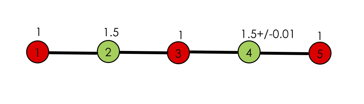
Figure 4: A chain of 5 weighted vertices. The weight of each vertex is indicated above the vertex, where vertex 4 has two possible values, either $w_{4}=1.5+0.01=1.51$ or $w_{4}=1.5-1.001=1.49$. Both $\{1,3,5\}$ (in red) and $\{2,4\}$ (in green) are the maximal independent set — weight$(\{1,3,5\})=3$; weight$(\{2,4\})=3.01$ when $w_{4}=1.51$ or $2.99$ when $w_{4}=1.49$. Thus, $\mathsf{mis}=\{1,3,5\}$ or $|\mathsf{GS}\rangle=|10101\rangle$ for $w_{4}=1.49$; while $\mathsf{mis}=\{2,4\}$ or $|\mathsf{GS}\rangle=|01010\rangle$ for $w_{4}=1.51$. They are complementary to each other.

There are two instances of this graph, one with $w_{4}=1.49$, another with $w_{4}=1.51$. Their solutions are complementary to each other by construction, namely, $\mathsf{mis}=\{1,3,5\}$ or $|\mathsf{GS}\rangle=|10101\rangle$ for $w_{4}=1.49$; while $\mathsf{mis}=\{2,4\}$ or $|\mathsf{GS}\rangle=|01010\rangle$ for $w_{4}=1.51$. Furthermore, these two instances are constructed so that the ground state of one instance is the first excited state of the other, and vice versa. Thus, the opposite result (the presence vs absence of an anti-crossing) is expected in the two instances.

In particular, the two instances have the opposite results for the min-gap when increasing the energy penalty $J$. More specifically, for the instance with $w_{4}=1.49$, when $J=1.52$, there is an anti-crossing resulting in a small min-gap, see Figure 5 for the detailed explanation; but as $J$ increases, the anti-crossing disappears and the min-gap is large, e.g. see Figure 6 for $J=4$. The opposite results are observed for the instance with $w_{4}=1.51$, see Figure 7 for the comparison of the results for $J=1.52$ (absence of the anti-crossing) vs $J=4$ (presence of the anti-crossing). The results of various $J$ $(1.52,4,10,100)$ for both instances with $w_{4}=1.49$ vs $w_{4}=1.51$ are compared side-by-side in Figure 8 (only the evolutions of $a_{k}$ are shown). For $w_{4}=1.49$ instance (left in Figure  8), increasing $J$ increases min-gap (anti-crossing disappears); while for $w_{4}=1.51$ instance (right in Figure  8), increasing $J$ decreases min-gap (anti-crossing appears).

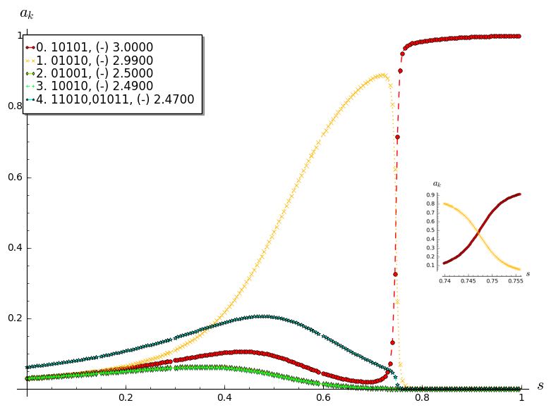
(a) Evolution of $a_{k}(s)$, $k=0,1,\ldots,4$

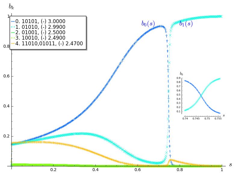
(b) Evolution of $b_{k}(s)$, $k=0,1,\ldots,4$

Figure 5: For the instance with $w_{4}=1.49$ and $J=1.52$. (a) Evolution of $a_{k}(s)$, where $a_{k}(s)=|\langle E_{k}(1)|{E_{0}(s)}\rangle|^{2}$ is the overlap of the $|E_{k}(1)\rangle$ with the ground state wavefunction $|E_{0}(s)\rangle$. The x-axis is the time $s$, and the y-axis is $a_{k}$. The lowest 5 levels ($0\leq k\leq 4$) are shown. The one in red is $a_{0}(s)$ and the one in orange is $a_{1}(s)$. In this instance, $s^{*}=0.7479,{\mathsf{mingap}}=0.0018$. the inset shows the occurrence of a $(0.15,0)$-Anti-crossing (with $\delta=0.008$) at $s^{*}$. In particular, within the zoom interval, $a_{0}(s)$ increases from $\sim 0.15$ to $\sim 0.85$; while $a_{1}(s)$ decreases from $\sim 0.85$ to $\sim 0.15$. At $s^{*}$, $a_{0}(s)=a_{1}(s)=0.5$. (b) Evolution of $b_{k}(s)$, where $b_{k}(s)=|\langle E_{k}(1)|{E_{1}(s)}\rangle|^{2}$ is the overlap of the $|E_{k}(1)\rangle$ with the first excited state wavefunction $|E_{1}(s)\rangle$. The one in blue is $b_{0}(s)$ and the one in cyan is $b_{1}(s)$. In the inset, $b_{1}(s)$ increases from $\sim 0.15$ to $\sim 0.85$; while $b_{0}(s)$ decreases from $\sim 0.85$ to $\sim 0.15$. At $s^{*}$, $b_{0}(s)=b_{1}(s)=0.5$. Together the above two plots demonstrate the presence of the anti-crossing at $s^{*}=0.7479$ where the min-gap occurs.

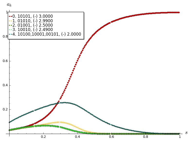
(a) Evolution of $a_{k}(s)$

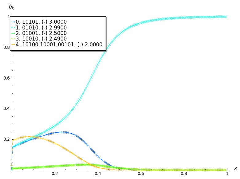
(b) Evolution of $b_{k}(s)$

Figure 6: For the instance with $w_{4}=1.49$ and $J=4$. (a) Evolution of $a_{k}(s)$, where $a_{k}(s)=|\langle E_{k}(1)|{E_{0}(s)}\rangle|^{2}$ is the overlap of the $|E_{k}(1)\rangle$ with the ground state wavefunction $|E_{0}(s)\rangle$. In this instance, $s^{*}=0.935,{\mathsf{mingap}}=0.0387$. There is no anti-crossing in this case, as one can see $a_{0}(s)$ increases steadily to $1$ at the end. (b) Evolution of $b_{k}(s)$, where $b_{k}(s)=|\langle E_{k}(1)|{E_{1}(s)}\rangle|^{2}$ is the overlap of the $|E_{k}(1)\rangle$ with the first excited state wavefunction $|E_{1}(s)\rangle$.

$$\begin{array}[h]{cc}\includegraphics[width=173.44534pt]{ab-w151-J152.jpg}&\includegraphics[width=173.44534pt]{ab-w151-J4.jpg}\\ (a)J=1.52&(b)J=4\end{array}$$

Figure 7: Evolution of $a_{0}(s),a_{1}(s),b_{0}(s),b_{1}(s)$ for the instance with $w_{4}=1.51$, where $a_{k}(s)=|\langle E_{k}(1)|{E_{0}(s)}\rangle|^{2}$ is the overlap of the $|E_{k}(1)\rangle$ with the ground state wavefunction $|E_{0}(s)\rangle$, ($a_{0}$ in red, $a_{1}$ in orange), $b_{k}(s)=|\langle E_{k}(1)|{E_{1}(s)}\rangle|^{2}$ is the overlap of the $|E_{k}(1)\rangle$ with the first excited state wavefunction $|E_{1}(s)\rangle$, ($b_{0}$ in blue, $b_{1}$ in cyan). (a) $J=1.52$: there is no anti-crossing. $a_{0}(s)$ and $b_{1}(s)$ keep increasing. (b) $J=4$: there is an anti-crossing.

$$\begin{array}[c]{l|l|l}&w_{4}=1.49,mis=\{1,3,5\}&w_{4}=1.51,mis=\{2,4\}\\ \hline\cr\\ J=1.52&s^{*}=0.7479,{\mathsf{mingap}}=0.0018&s^{*}=0.95,{\mathsf{mingap}}=0.03889\\ &\includegraphics[width=156.10345pt]{ak-w149-J152.jpg}&\includegraphics[width=156.10345pt]{ak-w151-J152.jpg}\\ \hline\cr\\ J=4&s^{*}=0.94,{\mathsf{mingap}}=0.0387&s^{*}=0.7262,{\mathsf{mingap}}=3.8e-4\\ &\includegraphics[width=156.10345pt]{ak-w149-J4.jpg}&\includegraphics[width=156.10345pt]{ak-w151-J4.jpg}\\ \hline\cr\\ J=10&s^{*}=0.95,{\mathsf{mingap}}=0.0389&s^{*}=0.7522,{\mathsf{mingap}}=1.2e-4\\ &\includegraphics[width=156.10345pt]{ak-w149-J10.jpg}&\includegraphics[width=156.10345pt]{ak-w151-J10.jpg}\\ \hline\cr\\ J=100&s^{*}=0.95,{\mathsf{mingap}}=0.0391&s^{*}=0.76147,{\mathsf{mingap}}=7.136e-5\end{array}$$

Figure 8: Evolution of $a_{k}(s)$ for two different instances ($w_{4}=1.49$ vs $w_{4}=1.51$) with various $J$. For $w_{4}=1.49$ instance (left), increasing $J$ increases min-gap (anti-crossing disappears); while for $w_{4}=1.51$ instance (right), increasing $J$ decreases min-gap (anti-crossing appears). Notice that for the same $J$ the results for the two instances with ($w_{4}=1.49$ vs $w_{4}=1.51$) are opposite (presence vs absence of the anti-crossing).

We now apply the LENS idea to explain our results. First, let us try to understand the result for the instance with $w_{4}=1.49,J=1.52$, where there is an anti-crossing as shown in Figure 5. In this example, $|\mathsf{GS}\rangle=|10101\rangle$ and $|\mathsf{FS}\rangle=|01010\rangle$. Among the 5 neighbors of $|\mathsf{GS}\rangle=|10101\rangle$, three of them $\{1010\underline{0},10\underline{0}01,\underline{0}0101\}$ are independent sets, of energy value $(-)2$. The other two $\{1\underline{1}101,101\underline{1}1\}$ are dependent sets of higher energy. Similarly, among the 5 neighbors of $|\mathsf{FS}\rangle=|01010\rangle$, there are two independent sets, and three dependent sets. The lowest 17 eigenstates of this instance are shown in Figure 9, where ${\mathsf{nbr}}_{{\mathcal{H}}_{\mathsf{X}}}(|0\rangle)=\{|5\rangle,|11\rangle,|12\rangle\}$ and ${\mathsf{nbr}}_{{\mathcal{H}}_{\mathsf{X}}}(|1\rangle)=\{|4\rangle,|9\rangle,|10\rangle,|16\rangle\}$. When restricting to the low-energy, we have ${\mathsf{lens}}_{{\mathcal{H}}_{\mathsf{X}}}(|0\rangle)=\{|5\rangle\}$ and ${\mathsf{lens}}_{{\mathcal{H}}_{\mathsf{X}}}(|1\rangle)=\{|4\rangle\}$. Since $|4\rangle$ is lower than $|5\rangle$, we say $|\mathsf{FS}\rangle$ has more LENS than $|\mathsf{GS}\rangle$ does. In this case, $a_{1}(s)$ increases faster as $s$ increases and becomes dominant before the anti-crossing.

However, when $J$ increases to $4$, the ranking of the neighboring states is changed. The lowest 17 eigenstates of this instance are shown in Figure 9 (b). Now we have ${\mathsf{nbr}}_{{\mathcal{H}}_{\mathsf{X}}}(|0\rangle)=\{|4\rangle,|15\rangle,|16\rangle\}$ and ${\mathsf{nbr}}_{{\mathcal{H}}_{\mathsf{X}}}(|1\rangle)=\{|5\rangle,|6\rangle,|9\rangle,|17\rangle\}$. When restricting to the low-energy, we have ${\mathsf{lens}}_{{\mathcal{H}}_{\mathsf{X}}}(|0\rangle)=\{|4\rangle\}$ and ${\mathsf{lens}}_{{\mathcal{H}}_{\mathsf{X}}}(|1\rangle)=\{|5\rangle,|6\rangle\}$. Thus, $|\mathsf{GS}\rangle$ has more LENS than $|\mathsf{FS}\rangle$ does, and $a_{0}(s)$ increases steadily and there is no anti-crossing, as shown in Figure 6.

$$\begin{array}[h]{cc}\includegraphics[width=173.44534pt]{nbrs-example-w149-152.jpg}&\includegraphics[width=173.44534pt]{nbrs-example-w149-4.jpg}\\ (a)&(b)\end{array}$$

Figure 9: The lowest 17 eigenstates of the instance with (a) $w_{4}=1.49$ and $J=1.52$ and (b) $w_{4}=1.49$ and $J=4$. The neighboring states of the ground state $|0\rangle$ (the first excited state $|1\rangle$, resp.) are in red (blue, resp.) rectangles. For (a), ${\mathsf{nbr}}_{{\mathcal{H}}_{\mathsf{X}}}(|0\rangle)=\{|5\rangle,|11\rangle,|12\rangle\}$ and ${\mathsf{nbr}}_{{\mathcal{H}}_{\mathsf{X}}}(|1\rangle)=\{|4\rangle,|9\rangle,|10\rangle,|16\rangle\}$. For (b), ${\mathsf{nbr}}_{{\mathcal{H}}_{\mathsf{X}}}(|0\rangle)=\{|4\rangle,|15\rangle,|16\rangle\}$ and ${\mathsf{nbr}}_{{\mathcal{H}}_{\mathsf{X}}}(|1\rangle)=\{|5\rangle,|6\rangle,|9\rangle,|17\rangle\}$.

In general, by increasing $J$, we increase the energy of the dependent set states, e.g., $\{|11010\rangle,|01011\rangle\}$, which are the neighboring states to $|01010\rangle$. If $J$ is increased such that $\{|11010\rangle,|01011\rangle\}$ becomes the high-energy state (from being the low-energy state), $|01010\rangle$ will then have less LENS. If $|01010\rangle$ is the ground state as in $w_{4}=1.51$ case, this will reduce the weight of $a_{0}(s)$ but increase the weight of $a_{1}(s)$ and force an anti-crossing. Conversely, if $|01010\rangle$ is the first excited state as in $w_{4}=1.49$ case, this will reduce the weight of $a_{1}(s)$ and $a_{0}(s)$ will keep increasing, and there is no anti-crossing. In our above example, for $J=1.52$, both $\{|11010\rangle,|01011\rangle\}$ are low in energy in eigenstate $|4\rangle$, which is a neighboring state to $|\mathsf{FS}\rangle$. Thus, $|\mathsf{FS}\rangle$ has more LENS than $|\mathsf{GS}\rangle$ does, $a_{1}(s)$ increases faster as $s$ increases and becomes dominant before the anti-crossing. However, for $J=4$, their energy increases to the eigenstate $|9\rangle$, and $\{|10100\rangle,|10001\rangle,|00101\rangle\}$ , which are the neighboring state to $|\mathsf{GS}\rangle$, becomes $|4\rangle$. Thus, $|\mathsf{GS}\rangle$ has more LENS than $|\mathsf{FS}\rangle$, and $a_{0}(s)$ increases steadily and there is no anti-crossing. As $J$ keeps increasing, it continues to increase the energy value of some dependent sets, but the low-energy neighborhood structure remains the same, and thus the evolution remains the same shape with a slight change in the gap size.

For a fixed $J$, we compare the two different $w_{4}$ instances (each row in Figure 8). Their results are opposite, one with an anti-crossing, and one without an anti-crossing. As we mentioned, this is to be expected. The ground state for one is the first excited state of the other, and vice versa. If there is no anti-crossing for one, the other will have an anti-crossing because the ground state of one instance will become the first excited state of the other instance to compete with its complement.

To further verify the neighborhood part of our LENS idea, we replace the $X$-driver ${\mathcal{H}}_{X}=-\sum_{i\in{\mathsf{V}}(G)}\sigma_{i}^{x}$ with a (stoquastic) $XX$-driver ${\mathcal{H}}_{XX}=-\sum_{i\in{\mathsf{V}}(G)}\sigma_{i}^{x}-\sum_{ij\in{\mathsf{E}}(G)}\sigma_{i}^{x}\sigma_{j}^{x}$ which has the uniform (with positive amplitudes) superposition state as the initial ground state, and thus our LENS idea applies. By changing from the $X$-driver to the $XX$-driver, the neighborhood will also include the two-bit flip neighbors. For example, the low energy states $|\underline{10}010\rangle$ and $|010\underline{01}\rangle$ become the neighboring (2-bit flip) states of $|01010\rangle$. If $|01010\rangle$ is the ground state as in $w_{4}=1.51$ case, $|\mathsf{GS}\rangle$ will have more LENS, $a_{0}(s)$ will increase faster, and there is no anti-crossing. But if $|01010\rangle$ is the first excited state as in the $w_{4}=1.49$ case, $|\mathsf{FS}\rangle$ will have more LENS, and this will reduce the weight of $a_{0}(s)$ but increase the weight of $a_{1}(s)$ and force an anti-crossing. For $w_{4}=1.51$, the opposite results when using $X$-driver vs $XX$-driver are as shown in Figure 10. However, for the same reason, $XX$-driver can also decrease the min-gap by introducing an anti-crossing while there is no anti-crossing with $X$-driver. See Figure 11 for the results for $w_{4}=1.49$, $J=4,10$. More discussion on the $XX$-driver Hamiltonians (both stoquastic and non-stoquastic) and the driver graphs can be found in [9].

$$\begin{array}[c]{l|l|l}&\mbox{X-driver: }{\mathcal{H}}_{X}=-\sum_{i\in{\mathsf{V}}(G)}\sigma_{i}^{x}&\mbox{XX-driver: }{\mathcal{H}}_{XX}=-\sum_{i\in{\mathsf{V}}(G)}\sigma_{i}^{x}-\sum_{ij\in{\mathsf{E}}(G)}\sigma_{i}^{x}\sigma_{j}^{x}\\ \hline\cr\\ J=4&s^{*}=0.7262,{\mathsf{mingap}}=3.8e-4&s^{*}=0.965,{\mathsf{mingap}}=0.03928\\ &\includegraphics[width=156.10345pt]{ak-w151-J4.jpg}&\includegraphics[width=156.10345pt]{ak-w151-J4-XX.jpg}\\ \hline\cr\\ J=10&s^{*}=0.7522,{\mathsf{mingap}}=1.2e-4&s^{*}=0.965,{\mathsf{mingap}}=0.039322\\ &\includegraphics[width=156.10345pt]{ak-w151-J10.jpg}&\includegraphics[width=156.10345pt]{ak-w151-J10-XX.jpg}\\ \end{array}$$

Figure 10: X-driver vs XX-driver for instance $w_{4}=1.51$. The anti-crossing is avoided with the $XX$-driver. This is because $|2\rangle=|\underline{10}010\rangle$ and $|3\rangle=|010\underline{01}\rangle$ become ${\mathsf{lens}}_{\mathsf{H_{XX}}}(|\mathsf{GS}\rangle)$ where $|\mathsf{GS}\rangle=|01010\rangle$. Thus, $|\mathsf{GS}\rangle$ has more LENS than $|\mathsf{FS}\rangle$ does.

$$\begin{array}[c]{l|l|l}&\mbox{X-driver: }{\mathcal{H}}_{X}=-\sum_{i\in{\mathsf{V}}(G)}\sigma_{i}^{x}&\mbox{XX-driver: }{\mathcal{H}}_{XX}=-\sum_{i\in{\mathsf{V}}(G)}\sigma_{i}^{x}-\sum_{ij\in{\mathsf{E}}(G)}\sigma_{i}^{x}\sigma_{j}^{x}\\ \hline\cr\\ J=4&s^{*}=0.94,{\mathsf{mingap}}=0.0387&s^{*}=0.82375,{\mathsf{mingap}}=0.016349]\\ &\includegraphics[width=156.10345pt]{ak-w149-J4.jpg}&\includegraphics[width=156.10345pt]{ak-w149-J4-XX.jpg}\\ \hline\cr\\ J=10&s^{*}=0.95,{\mathsf{mingap}}=0.0389&s^{*}=0.81759,{\mathsf{mingap}}=0.013135\\ &\includegraphics[width=156.10345pt]{ak-w149-J10.jpg}&\includegraphics[width=156.10345pt]{ak-w149-J10-XX.jpg}\\ \end{array}$$

Figure 11: X-driver vs XX-driver for instance $w_{4}=1.49$. The $XX$-driver in this case decrease the min-gap with a weak anti-crossing. This is because $|2\rangle=|\underline{10}010\rangle$ and $|3\rangle=|010\underline{01}\rangle$ become ${\mathsf{lens}}_{\mathsf{H_{XX}}}(|\mathsf{FS}\rangle)$ where $|\mathsf{FS}\rangle=|01010\rangle$. It is a weak anti-crossing because the min-gap does not happen at $0.5$ anti-crossing point, and also the left boundary does not sum up to one: there are other non-negligible states besides $|\mathsf{GS}\rangle$ and $|\mathsf{FS}\rangle$.

4.2 Example 2: Anti-crossings remain

We construct this example to show that it is not always sufficient that increasing the energy penalty $J$ will remove anti-crossings. This example is constructed to further verify our LENS idea. The input graph is a chain of 7 qubits as shown in Figure 12. The results with different $J$ are shown in Figure 13. Recall that increasing $J$ will increase the energy of the dependent set states. However, this example is so constructed that all the low-energy states are independent sets, and thus, increasing $J$ only increases the already high-energy neighboring states, and thus it does not effectively change LENS. Furthermore, the states among the low-energy spectrum are at least 3 bit-flips from either $|\mathsf{GS}\rangle$ or $|\mathsf{FS}\rangle$, therefore changing to the stoquastic $XX$-driver Hamiltonian does not help. Indeed, in this example, the lowest 6 states remain the same even if with a larger $J$ value, or using a larger neighborhood.

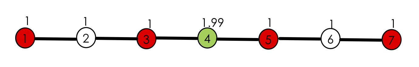
Figure 12: A chain of 7 weighted vertices. The weight of each vertex is indicated above the vertex, where vertex $w_{4}=1.99$ and all other vertex has weight 1. The mis is $\{1,3,5,7\}$ with wight $4$. But there are a 4-fold degenerate local minima $\{146,246,147,247\}$, with weight $3.99$.

$$\begin{array}[c]{ll}J=2,s^{*}=0.84375,{\mathsf{mingap}}=0.00155&J=10,s^{*}=0.70609,{\mathsf{mingap}}=0.00413683\\ \includegraphics[width=216.81pt]{C7-J2.jpg}&\includegraphics[width=216.81pt]{C7-J10.jpg}\\ J=100,s^{*}=0.6456,{\mathsf{mingap}}=0.0074294&J=1000,s^{*}=0.6389,{\mathsf{mingap}}=0.0080297\\ \end{array}$$

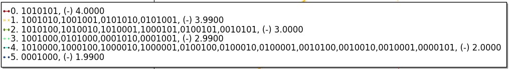
Figure 13: Different $J$ for the chain-7 instance in Figure 12. The lowest 5 states consist of all independent set states and remain the same for any $J$. The increase in the min-gap as $J$ increases is mainly due to the scaling.

Remark.

The arguments made by Dickson and Amin in [10] to remove the perturbative crossings do not apply to the above two examples. Take for instance the $w_{4}=1.51$ instance in Example 1. In this example there is no degeneracy. Increasing $J$ actually introduces the presence of an anti-crossing and decreases the min-gap: the opposite of their argument that it would eliminate the perturbative crossing and increase the min-gap. There are two main differences: (1) Our anti-crossing is more general than the perturbative crossing which only applies to the perturbation at the end of evolution with respect to the problem Hamiltonian. (2) Our example is for the weighted MIS problem, while the argument there is for the unweighted MIS problem.

5 Scaling the Problem Hamiltonian

In this section, we investigate how the minimum spectral gap of a scaled Hamiltonian $H^{\alpha}$ varies according to the parameter $\alpha$. In particular, we consider the $\alpha$-scaled Hamiltonian:

$$H^{\alpha}(t)=(1-t)H_{B}+t\alpha\cdot H_{P}$$ (13)

where $t\in[0,1]$, $\alpha>1$. (Remark: We consider $\alpha>1$, and will compare $H^{\alpha}$ with $H^{1}$. In the case $\alpha<1$, one can compare $H^{\alpha}$ with $(H^{\alpha})^{1/\alpha}$.) Let $H^{1}=H(s)=(1-s)H_{B}+sH_{P}$ where $s\in[0,1]$.

Theorem 5.1.

1. There is one-one correspondence between $s$ and $t$. Namely, for $s\in[0,1)$, $t(s)=\frac{s}{\alpha(1-s)+s}$. Conversely, for $t\in[0,1)$, $s(t)=\frac{t\alpha}{1+(\alpha-1)t}$.

2. The eigen-energies are scaled, and the eigenstates are preserved:

   $$E_{i}^{\alpha}(t)=(1+(\alpha-1)t)E_{i}(s(t))$$ (14)

   where $E_{i}^{\alpha}(t)$ ($E_{i}(s(t))$ resp.) are the $i$th eigenvalue of $H^{\alpha}(t)$ ($H(s(t))$ resp.), for all $i$. Furthermore, $|E_{i}^{\alpha}(t)\rangle=|E_{i}(s(t))\rangle$, for all $i$.

3. The min-gap is scaled, and the min-gap position is shifted:

   $${\mathsf{mingap}}(H^{\alpha})=(1+f(\alpha)){\mathsf{mingap}}(H^{1})$$

   where $f(\alpha))=(\alpha-1)t^{\prime}>0$, with $t^{*}\leq t^{\prime}\leq t(s^{*})$, $t^{*}$ ($s^{*}$ resp. ) is the position of the minimum gap of $H^{\alpha}$ ($H^{1}$ resp.), and $t(s)=\frac{s}{\alpha(1-s)+s}$ for $s\in[0,1)$. Moreover, $t^{*}\leq t(s^{*})<s^{*}$.

Proof.

Let $H(s)=(1-s)H_{B}+sH_{P}$ where $s\in[0,1]$. We will show there is one-one correspondence between $s\in[0,1)$ in $H(s)$ and $t\in[0,1)$ in $H^{\alpha}(t)$. Consider

$$\left\{\begin{array}[]{l}\frac{H(s)}{1-s}=H_{B}+\frac{s}{1-s}H_{P}\\ \frac{H^{\alpha}(t)}{1-t}=H_{B}+\frac{t\alpha}{1-t}H_{P}\end{array}\right.$$

Solving $\frac{s}{1-s}=\frac{t\alpha}{1-t}$, we get $s(t):=s=\frac{t\alpha}{1+(\alpha-1)t}\in[0,1)$, and $t(s):=t=\frac{s}{\alpha(1-s)+s}\in[0,1)$. Notice that $s(t)$ and $t(s)$ are the bijections and inverse of each other.

Thus, we have

$$\frac{H^{\alpha}(t)}{1-t}=\frac{H(s)}{1-s}$$

where $s=s(t)$ or $t=t(s)$.

Since $\frac{1-t}{1-s}=\frac{1-t}{1-\frac{t\alpha}{1+(\alpha-1)t}}=1+(\alpha-1)t$, we have

$$H^{\alpha}(t)=\frac{1-t}{1-s}H(s)=(1+(\alpha-1)t)H(s)$$ (15)

Therefore, we have

$$E_{i}^{\alpha}(t)=(1+(\alpha-1)t)E_{i}(s(t))$$ (16)

where $E_{i}^{\alpha}(t)$ ($E_{i}(s(t))$ resp.) are the $i$th eigenvalue of $H^{\alpha}(t)$ ($H(s(t))$ resp.). Also, $|E_{i}^{\alpha}(t)\rangle=|E_{i}(s(t))\rangle$. In particular, ${\mathsf{mingap}}(H^{\alpha})=(1+(\alpha-1)t^{*})\mbox{gap}_{H}(s(t^{*}))\geq(1+(\alpha-1)t^{*}){\mathsf{mingap}}(H)$.

Similarly, ${\mathsf{mingap}}(H^{\alpha})\leq\mbox{gap}_{H^{\alpha}}(t(s^{*}))=(1+(\alpha-1)t(s^{*})){\mathsf{mingap}}(H)$.

Next we show that $t^{*}\leq t(s^{*})<s^{*}$.

Since $\alpha>1$, $t(s)=\frac{s}{\alpha(1-s)+s}<\frac{s}{(1-s)+s}=s$, in particular $t(s^{*})<s^{*}$.

From Eq. (16),

$$\left\{\begin{array}[]{ll}\mbox{gap}_{H^{\alpha}}(t(s^{*}))&=(1+(\alpha-1)t(s^{*}))\mbox{gap}_{H}(s^{*})\\ \mbox{gap}_{H^{\alpha}}(t^{*})&=(1+(\alpha-1)t^{*})\mbox{gap}_{H}(s(t^{*}))\end{array}\right.$$

Since ${\mathsf{mingap}}(H)=\mbox{gap}_{H}(s^{*})\leq\mbox{gap}_{H}(s(t^{*}))$, if $t(s^{*})<t^{*}$, it would imply $\mbox{gap}_{H^{\alpha}}(t(s^{*}))<(1+(\alpha-1)t^{*})\mbox{gap}_{H}(s^{*})=(1+(\alpha-1)t^{*}){\mathsf{mingap}}(H)<(1+(\alpha-1)t^{*})\mbox{gap}_{H}(s(t^{*}))<\mbox{gap}_{H^{\alpha}}(t^{*})={\mathsf{mingap}}(H^{\alpha})$ a contradiction. ∎

Remarks:

• The above theorem implies that for $\alpha>1$, the minimum gap increases as $\alpha$ increases.

• Notice that $t(s^{*})$ and $t^{*}$ are not necessarily the same. For $\alpha>1$, $t^{*}\leq t(s^{*})<s^{*}$. This implies that by increasing $\alpha$, we also push the position of the minimum gap towards $0$. This is because when $\alpha$ is large, $t^{*}\leq t(s^{*})=\frac{s^{*}}{\alpha(1-s^{*})+s^{*}}\leadsto 0$. This may also pose a physical limitation of the value of $\alpha$ as too close to zero may shorten the “quantum phase”.

• If we allow infinite energy value, e.g. by setting $\alpha=1+K/t(s^{*})$, for an arbitrarily large $K$, we have ${\mathsf{mingap}}(H^{\alpha})\geq(1+K){\mathsf{mingap}}(H^{1})$. That is, if we allow infinite energy value (which is unrealistic), we can have the min-gap arbitrarily large.

Anti-crossing preserved under scaling.

If the curvature around the min-gap is sharp(as in the exponentially small gap case), $t^{*}=t(s^{*})$, and $s(t^{*})=s^{*}$. Then,

$${\mathsf{mingap}}(H^{\alpha})=(1+(\alpha-1)t(s^{*})){\mathsf{mingap}}(H^{1}).$$ (17)

What is more, $|E_{0}^{\alpha}(t^{*})\rangle=|E_{0}(s^{*})\rangle$. Hence the presence of the anti-crossing will be preserved under our parametrized definition. To illustrate, we use $w_{4}=1.51,J=10$ in Example 1. The scaling or renormalizing factor is $\alpha=10$. The comparison is shown in Figure 14. Furthermore, if it is a weak anti-crossing, by scaling, one can not make it to a (strong) anti-crossing.

Renormalization.

When comparing the performance of different parameter QA algorithms, there is an argument that one needs to renormalize the problem Hamiltonian so that the largest parameter is of the same value. Indeed, scaling/renormalizing the problem Hamiltonian will change the min-gap according to our above theorem. As we show in Figure 14, we know exactly how much the contribution to the min-gap is due to the scaling (according to Eq (17)), and how much is due to the difference in the parameters. Hence, there is no such need for renormalization, when one can use the parameter value as it is.

$$\begin{array}[h]{cc}\includegraphics[width=173.44534pt]{scaling-w151-J10.jpg}&\includegraphics[width=173.44534pt]{scaling-w151-J10-01.jpg}\\ (a)\alpha=10&(b)\alpha=1\end{array}$$

Figure 14: Evolution of $a_{k}(s)$ for the instance with $w_{4}=1.51$, and $J=10$ of Example 1. The $(\gamma,\epsilon)$-Anti-crossing is preserved with two different scaling factors (a) $\alpha=10$ and (b) $\alpha=1$, where $\epsilon=0$ and $\gamma\leq 0.001$ for both, $\delta=0.02$ for (a), but $\delta=0.002$ for (b). Moreover, (a) $t^{*}=0.7522$, ${\mathsf{mingap}}=1.2e-4$; and (b) $s^{*}=0.9681$, ${\mathsf{mingap}}=1.566e-5$. One can check that $t^{*}=t(s^{*})$, the min-gaps satisfy ${\mathsf{mingap}}(H^{\alpha})=(1+(\alpha-1)t(s^{*})){\mathsf{mingap}}(H^{1})$, where the factor $(1+(\alpha-1)t(s^{*})=7.7698$, $\alpha=10$.

6 Summary and Discussion

In this paper, we show that the problem Hamiltonian parameters can affect the minimum spectral gap of the adiabatic algorithm. The main argument we use to assess the performance of a QA algorithm is the presence or absence of an anti-crossing during quantum evolution. For this purpose, we introduce a new parametrization definition of the anti-crossing. Our definition allows us to characterize or provide a signature for identifying an anti-crossing based on the numerical diagonalization of the Hamiltonian. This is in contrast to other numerical studies that compute the min-gaps for some small number of instances of size up to 20, and then best fit the data with some exponentially small function (see e.g. Figure 2). Besides, sometimes the evidence of quantum tunneling that was quantified by a sharp change in the ground state expectation of the Hamming weight operator $\langle HW\rangle$, such as Figure 6 in [1], was presented for further justification. Anti-crossing is intimately related to the quantum tunneling. Indeed, the loop-gadgets example was constructed to have small anti-crossing gaps in order to show the evidence of the quantum tunneling. As we remarked, our anti-crossing definition readily gives rise to the values of the Hamming weight operator $\langle HW\rangle$. Our anti-crossing definition reflects the known concept of the anti-crossing (c.f. [19]) and is more general than the perturbative crossing in [4, 10]. A perturbative crossing is necessarily an anti-crossing, but an anti-crossing is not necessarily a perturbative crossing which is limited to the location near the end of evolution when the perturbation theory is applied to the problem Hamiltonian as the unperturbed Hamiltonian. In [4], an estimation formula of the min-gap size was given based on the perturbation theory. We are investigating how to estimate the min-gap size based on this more general anti-crossing definition.

Based on our LENS observation that the presence or absence of an anti-crossing depends on the relation of the ground state and the first excited state with their LENS, we construct two Maximum-weighted Independent Set (MIS) examples to answer the questions we study. More specifically, we construct Example 1 to show that one can change the energy penalty parameter $J$ (without changing the problem to be solved) to change the quantum evolution (from the presence of an anti-crossing to the absence, or the other way around). However, we also show in Example 2 that by changing the value of $J$ alone, one can not avoid the anti-crossing. The examples we construct are of small sizes for easy illustration. It is not difficult to construct a larger size of instances such that the argument still holds (e.g. one can construct instances which contain our small graph as subgraphs). Admittedly, our LENS idea is still premature and incomplete because the general situation can be much more complex, with many more anti-crossings. Nevertheless, for what its worth, we believe that this simple observation is useful to give some understanding of the working of the QA algorithm, especially in this early stage of QA research where rigorous small experimental tests are needed. Moreover, by understanding the causes of the formation of the anti-crossing, one can also learn to come up with possible ways of avoiding such bottlenecks, as we show in our Example 1.

We construct our examples of the MIS problem because it has a natural parameter-flexible Ising formulation. However, our results do not lose generality because any Ising problem can be easily and efficiently reduced to the parameter-flexible MIS-Ising Hamiltonian and thus also allow the flexibility to change the parameters without changing the problem to be solved. Based on our results, one possible advantage of expressing as an MIS-Ising Hamiltonian is then that one may adaptively re-run the program based on the measured output to improve the performance. For example, one idea is as follows: assume that the output state $|\phi\rangle$ is $|\mathsf{FS}\rangle$ (which has more LENS according to the original setting). We then increase the energy penalty of $|\phi\rangle$’s neighbors (again we can do so because of the MIS-Ising Hamiltonian). This will effectively increase $|\phi\rangle$’s neighboring states (dependent set) in the next run, and thus discourage the state from becoming dominant in the early evolution if $|\phi\rangle$ is not the true ground state. In the case of Example 1, it is possible to improve the algorithm performance. However, as we show in Example 2, this is not always sufficient to remove the anti-crossing.

We also show exactly how the min-gap is scaled if we scale the problem Hamiltonian by a constant factor. In particular, one can increase the min-gap to arbitrarily large if the energy value could be infinite (which is unphysical). Furthermore, our result implies that there is no need for renormalization of the parameters in order for the comparison of different parameter QA algorithms. These results are to raise attention to the importance of the dynamic range/precision/resolution of the parameters for the quantum annealer, and also to re-iterate the possibilities of different input formulation (either with different parameter values or through some NP-complete reductions as discussed in [7]) for the same problem, which may also pose a challenge to the benchmarking task.

The driver Hamiltonians we study in this paper are known as stoquastic Hamiltonians (we use the property that their ground state is the uniform superposition state with all positive amplitudes so that our LENS idea applies). There are arguments that the stoquastic Hamiltonian system can be efficiently simulated by quantum Monte Carlo (QMC), see [1, 14, 13, 15] and references therein. On the other hand, there are examples [4, 3] that show that the quantum annealing algorithm with the transverse-field driver Hamiltonian and a certain formulation of the problem Hamiltonian will take exponential time because of the presence of anti-crossings. While one may eliminate the perturbative crossings [10, 11], the question of eliminating the more general anti-crossings remains open. Perhaps the advantage of QA algorithms for the stoquastic Hamiltonian system over the classical algorithms for the NP-hard optimization problem is questionable (e.g. because of the efficient QMC simulation). Nevertheless, from the algorithmic point of view, it is still of the value to better understand the working of the QA algorithm. For example, by understanding the causes of the formation of an anti-crossing, one may be able to come up with possible ways to overcome them (such as what we show here by changing the parameter values), and this will directly (through the QMC simulation) result in an efficient quantum-inspired classical algorithm for these problem instances. Furthermore, it is possible to gain insight from the stoquastic Hamiltonian system and design the corresponding non-stoquastic counterpart to overcome the anti-crossing problem as we discuss in [9], where we study both stoquastic and non-stoquastic $XX$-driver Hamiltonians and different driver graphs and show their effects on the quantum evolution of the QA algorithm.

Finally, we remark that there is a work of quantum speedup in stoquastic adiabatic quantum computation (stoqAQC) in [12]. The proposed stoqAQC model there requires non-standard basis measurements and demands high-quality qubits, and quantum error correction which is necessary for any quantum computing device, to achieve the speedup.

References

- [1] T. Albash. Role of Non-stoquastic Catalysts in Quantum Adiabatic Optimization. Phys. Rev. A., 99, 042334, 2019.
- [2] T. Albash and D.A. Lidar. Adiabatic Quantum Computation. Rev. Mod. Phys. 90, 015002, 2018.
- [3] B. Altshuler, H Krovi, J Roland. Anderson localization makes adiabatic quantum optimization fail. Proc Natl Acad Sci USA, 107:12446–12450, 2010.
- [4] M.H.S. Amin, V. Choi. First order phase transition in adiabatic quantum computation. arXiv:quant-ph/0904.1387. Phys. Rev. A., 80 (6), 2009.
- [5] E. Boros, P.L. Hammer. Pseudo-Boolean optimization. Discrete Applied Mathematics, 123, 155–-225, 2002.
- [6] V. Choi. Different Adiabatic Quantum Algorithms for the NP-Complete Exact Cover Problem. Proc Natl Acad Sci USA, 108(7): E19-E20, 2011.
- [7] V. Choi. Different Adiabatic Quantum Algorithms for the NP-Complete Exact Cover and 3SAT Problem. arXiv:quant-ph/1010.1221. Quantum Information and Computation, Vol. 11, 0638–0648, 2011.
- [8] V. Choi. Minor-embedding in adiabatic quantum computation: I. The parameter setting problem. Quantum Inf. Processing., 7, 193–209, 2008.
- [9] V. Choi. XX-Driver Hamiltonian and Driver Architecture in Adiabatic Quantum Optimization. In preparation, 2019.
- [10] N.G. Dickson, M.H.S. Amin. Does Adiabatic Quantum Optimization Fail for NP-complete Problems? Phys. Rev. Lett. 106, 050502, 2011.
- [11] N. G. Dickson. Elimination of perturbative crossings in adiabatic quantum optimization, New Journal of Physics 13, 073011, 2011.
- [12] K. Fujii. Quantum speedup in stoquastic adiabatic quantum computation. arXiv:1803.09954, 2018.
- [13] M. B. Hastings and M. H. Freedman. Obstructions to classically simulating the quantum adiabatic algorithm, arXiv:1302.5733, 2013.
- [14] L. Hormozi, E. W. Brown, G. Carleo, and M. Troyer. Nonstoquastic hamiltonians and quantum annealing of an ising spin glass, Phys. Rev. B 95, 184416, 2017.
- [15] M. Jarret, S. P. Jordan, and B. Lackey. Adiabatic optimization versus diffusion monte carlo methods, Physical Review A 94, 042318, 2016.
- [16] S. Muthukrishnan, T. Albash, and D.A. Lidar. Tunneling and speedup in quantum optimization for permutation-symmetric problems. arXiv:quant-ph/1511.03910, Phys. Rev. X, 6, 031010, 2016.
- [17] M. A. Qureshi, J. Zhong, P. Mason, J. J. Betouras,and A. M. Zagoskin. Pechukas-Yukawa formalism for Landau-Zener transitions in the presence of external noise. arXiv:1803.05034v2, 2018.
- [18] W. A. Stein et al., Sage Mathematics Software (Version 8.0). The Sage Development Team, 2009, http://www.sagemath.org.
- [19] M. Wilkinson, Statistical aspects of dissipation by Landau-Zener transitions. J. Phys. A: Math. Gen., 21, 4021-4037, 1988.
- [20] M. Wilkinson, Statistics of multiple avoided crossings. J. Phys. A: Math. Gen., 22, 2795-2805, 1989.