The Magnet of the Scattering and Neutrino Detector for the SHiP experiment at CERN

Abstract

The Search for Hidden Particles (SHiP) experiment proposal at CERN demands a dedicated dipole magnet for its scattering and neutrino detector. This requires a very large volume to be uniformly magnetized at $B>1.2$ T, with constraints regarding the inner instrumented volume as well as the external region, where no massive structures are allowed and only an extremely low stray field is admitted. In this paper we report the main technical challenges and the relevant design options providing a comprehensive design for the magnet of the SHiP Scattering and Neutrino Detector.

1 Introduction

Given the absence of direct experimental evidence for Beyond the Standard Model (BSM) physics at the high-energy frontier and the lack of unambiguous experimental hints for the scale of new physics in precision measurements, it might well be that the shortcomings of the Standard Model (SM) have their origin in new physics involving very weakly interacting, relatively light particles. As a consequence of the extremely feeble couplings and the typically long lifetimes, the low mass scales for hidden particles are far less constrained [1]. In several cases, the present experimental and theoretical constraints from cosmology and astrophysics indicate that a large fraction of the interesting parameter space was beyond the reach of previous searches, but it is open and accessible to current and future facilities. While the mass range up to the kaon mass has been the subject of intensive searches, the bounds on the interaction strength of long-lived particles above this scale are significantly weaker. The recently proposed Search for Hidden Particles (SHiP) beam-dump experiment [2] at the CERN Super Proton Synchrotron (SPS) accelerator is designed to both search for decay signatures by full reconstruction and particle identification of SM final states and to search for scattering signatures of Light Dark Matter by the detection of recoil of atomic electrons or nuclei.

The Beam Dump Facility (BDF) where SHiP operates is well described in ref. [3]: the most upstream BDF part is a proton target followed by a 5 m long hadron absorber. In addition to absorbing the hadrons and the electromagnetic radiation, the iron of the hadron absorber is magnetised over a length of 4 m. Its dipole field makes up the first section of the active muon shield [4] which is optimised to sweep out of acceptance muons of the entire momentum spectrum, up to 350 GeV/$c$. The remaining part of the muon shield follows immediately downstream of the hadron absorber in the experimental hall and consists of a chain of iron core magnets which extends over a length of about 30 m.

The SHiP experiment incorporates two complementary apparatuses. The detector system immediately downstream of the muon shield is optimised both for recoil signatures of hidden sector particle scattering and for neutrino physics. It is based on a hybrid detector with a concept similar to what was developed by the OPERA Collaboration [5] with alternating layers of nuclear emulsion films with high-density $\nu$-target plates and electronic trackers. In addition, the detector is located in a magnetic field for charge sign and momentum measurement of hadronic final states. The detector $\nu$-target mass totals about 10 tons. The emulsion spectrometer is followed by a muon identification system. It also acts as a tagger for interactions in its passive layers which may produce long-lived neutral mesons entering the downstream decay volume and whose decay may mimic signal events. The second detector system aims at measuring the visible decays of Hidden Sector particles to both fully reconstructible final states and to partially reconstructible final states with neutrinos. The detector consists of a 50 m long decay volume followed by a large spectrometer with a rectangular acceptance of 5 m in width and 10 m in height [3]. The spectrometer is designed to accurately reconstruct the decay vertex, the mass, and the impact parameter of the hidden particle trajectory at the proton target. A calorimeter and a muon identification system provide particle identification. A dedicated timing detector with $\sim$100 ps resolution provides a measure of coincidence in order to reject combinatorial backgrounds. The decay volume is surrounded by background taggers to identify neutrino and muon inelastic scattering in the vacuum vessel walls. The muon shield and the SHiP detector systems are housed in a $\sim$120 m long underground experimental hall at a depth of $\sim$15 m.

In this paper we report the design and the expected performance of the SND magnet, which contains the hybrid apparatus of the Scattering and Neutrino Detector. The work is organized as follows. In section 2 the experimental requirements at the basis of the overall design constraints are presented. In section 3 the full electromagnetic design is considered, from analytical models to 3-D numerical simulations, defining a viable design option. In section 4 the problem of mechanical forces and stresses are tackled, along with functional issues relevant to the final mechanical structure of the SND magnet. Finally section 5 draws the conclusions.

2 Experimental requirements

The design of the SHiP SND magnet follows the need for a significantly large, uniformly magnetized volume, in order to accommodate the $\nu$-target and the spectrometer trackers. This results in a magnetized volume of about 10 m³ with a magnetic field of at least 1.2 T. The lower bound on the field strength comes from the requirement to measure the charge sign and momentum of hadrons up to 10 GeV/$c$ in a very compact structure, the so-called Compact Emulsion Spectrometer (CES) [6], made of 3 emulsion films interleaved with air over a total thickness of 3 cm. At the same time, the stray field outside the magnet has to be sufficiently low (at the percent level of the inner value) to avoid disturbing the flux of muons swept out by the muon shield. This sets severe constraints on the shape and size of the magnet. In particular the magnet yoke, beside its fundamental magnetic role (increasing efficiency, homogenizing and straightening up the field) and the mechanical one (contrasting the strong magnetic expanding force acting on the coil), is expected to sufficiently shield the field outside the magnet. Such a requirement strongly affect the magnet design constraints and goals. The detector mass and its operating temperature as well as the accessibility for the detector installation and maintenance provide further challenges for the overall design. In particular, the CES is supposed to be replaced every few weeks in order to limit the total integrated flux of background muons, thus suppressing the combinatorial background in the track matching required for the sagitta measurement. That imply that the magnet has to be designed so that it can be frequently opened, approximately once a fortnight.

The required flux density over such a significant gap size requires a power of about 1 MW. In the past, at CERN, experimental magnets of comparable or even higher power consumption (e.g. LHCb  [7, 8, 9] is 4.2 MW) were designed resistive to favour a much easier operation. Furthermore, in this specific case, the CES will have to be replaced every few weeks and this will require easy human accessibility, certainly more difficult in presence of helium and of a cryogenic infrastructure. The resistive design reported here would however consume only one fourth of the LHCb magnet, making the drawbacks of a superconducting version, including constructional difficulties, far more remarkable. This is why for the baseline design we adopt a reliable and well-established design with resistive coils. However, the study of a superconducting magnet will also be carried out, as an option to the baseline design. One of the directions we intend to explore is an innovative concept of cryogen free magnet [10] using HTS conductors, or alternatively LTS coils indirectly cooled with a small inventory of liquid helium. This goes beyond the scope of this paper.

The power converter system and more generally any ancillary equipment have to comply with CERN standard specifications. Table 1 reports the main specifications of the magnet.

Table 1: Magnet Specifications.

internal volume (detectors + ancillary equipment)		[m3]	$1\times 1.6\times 5.4$
overall external size		[m3]	$2.4\times 4.0\times 7.2$
internal volume temperature		[∘C]	$18$
reference field (internal volume)	$B$	[T]	$>1.2$
spatial field homogeneity (internal volume)	$\lvert\Delta B/B\rvert$	[%]	$\approx 1$
temporal field stability (internal volume)	$\lvert\Delta B/B\rvert$	[ppm]	$<10^{3}$
maximum external stray field	$B_{\text{stray\,max}}$	[mT]	$\leq 10$

3 Magnet design

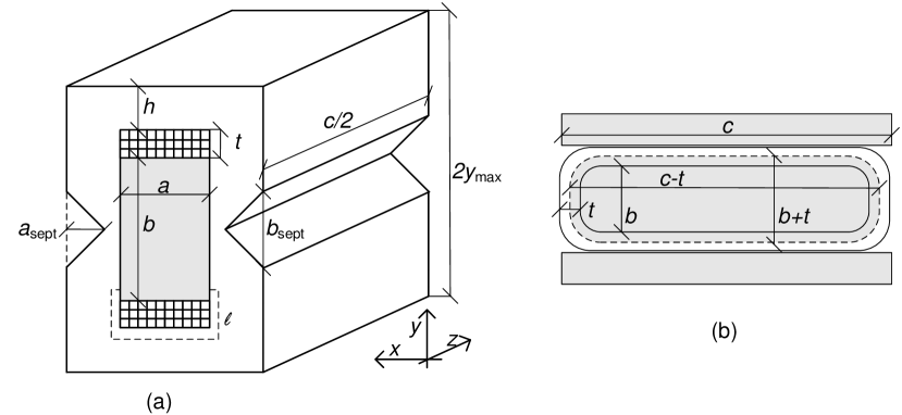
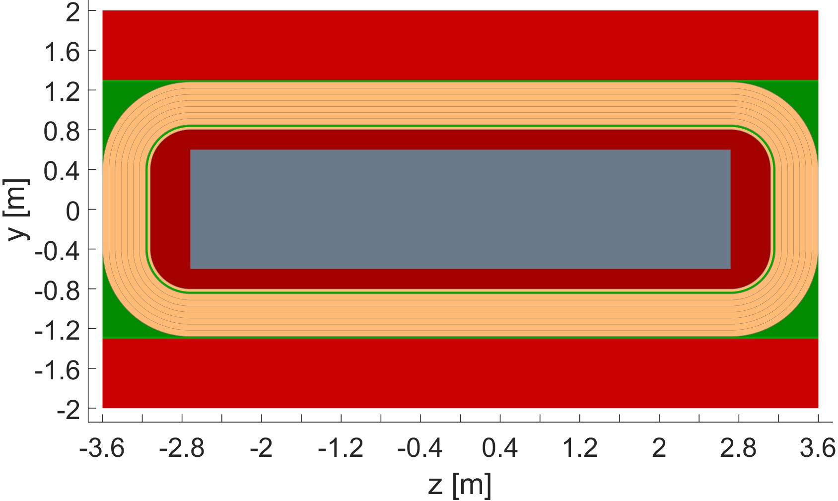
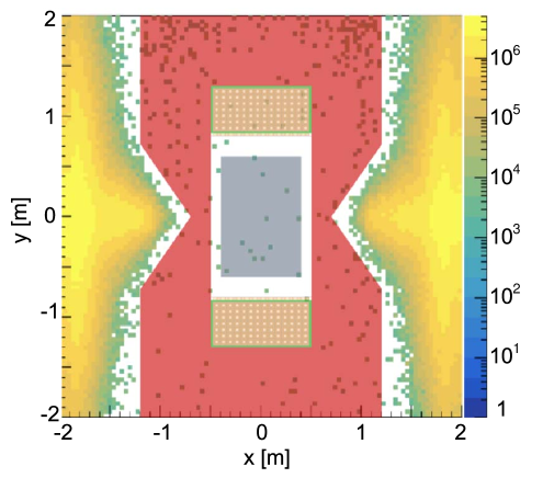
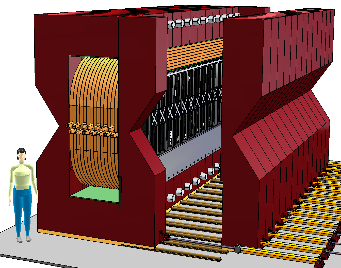
Figure 1a shows the simulated profile of the muon flux distribution in the transverse plane of the region where the SND detector is located. Such distribution sets the fundamental constraint on the transverse shape of the magnet that does not have to intercept the muon flux. From this feature, the magnet coil can be developed longitudinally, thus providing a horizontal field and the inner magnetised volume can be taller than wider. A conceptual design of the magnet is shown in figure 1b where the yoke shape is tapered according to the muon flux. Figure 2 shows a sketch of the magnet structure, with the definition of major geometrical parameters.

Figure 1: a) Simulated muons flux at the SND magnet position of the beam line. b) Sketch of the magnet’s cross-section.

Figure 2: (a) Schematic representation of one half of the magnet, showing the cross-section $z=0$ and the corresponding geometrical parameters. The point $x=y=z=0$ represents the centre of the magnet. The total magnet length along the direction of the beam (the $z$ direction) is equal to $c$. (b) Schematic $x=0$ cross-section, showing the areas (gray) considered for the flux balance.

3.1 Analytical formulae

We describe now the procedure to get an approximate analytical magnetic model, providing the basis for sizing the magnet. The results of such analysis are then employed as the starting guess for the detailed analysis that is performed in section 3.2, including the electrical and thermal coil design.

The standard design technique which seeks the optimal current density, leading to total cost minimization [11], cannot be adopted here. In fact, we have a prescription on the maximum possible total magnet height, which is fixed at $2y_{\text{max}}\cong 4$ m. This is determined by the muons profile, which also sets the maximum tolerable external field $B_{\text{stray\,max}}$ (table 1). The following analysis aims at determining design solutions that satisfy the (internal and external) dimensional constraints and the stray field specification, while minimizing the power.

With reference to figure 2 we recognize the following fundamental geometric constraint involving the coil and yoke thickness $t$ and $h$

$$\frac{b}{2}+t+h=y_{\text{max}}$$ (3.1)

where $b=1.6$ m is the total height of the magnetized volume and $c=7.2$ m is the magnet longitudinal length.

By neglecting the stray flux, which is a reasonable assumption for a well designed yoke, the flux is balanced when the internal flux $\phi_{\text{int}}$, that is the sum of the fluxes corresponding to the gap and to the coil, is equal to the flux into the yoke $\phi_{\text{Fe}}$. That is easily done by considering the $x=0$ cross-section of the magnet (figure 2b). The flux density in the coil decays approximately linearly, from the value $B$ at the internal edge to zero at the outer edge. The flux in the coil, per unit length, is hence given by product $Bt/2$. One then gets $\phi_{\text{int}}=(c-t)(b+t)B$, where the product $(c-t)(b+t)$ is an average area that takes into account the non uniformity of the flux density in the coil. The flux balance equation $\phi_{\text{int}}=\phi_{\text{Fe}}$ then reads as

$$(c-t)(b+t)B=2hc{B_{\text{Fe\,max}}},$$ (3.2)

where $B_{\text{Fe\,max}}$ is the maximum value of the flux density, attained in the top (and bottom) part of the yoke.

At this point we need to introduce the main figures of merit of the design, that are magnet efficiency, electrical power, magneto-motive force and stray field.

The magnet efficiency is defined as the ratio between the magnetic tension over the gap and the magneto-motive force (MMF), or formally [12, 13]

$$\eta={\frac{aB/\mu_{0}}{NI}}=\frac{\int_{\text{gap}}\bm{H}\cdot\mathrm{d}\bm{\ell}}{\int_{\text{gap}}\bm{H}\cdot\mathrm{d}\bm{\ell}+\int_{\text{iron}}\bm{H}\cdot\mathrm{d}\bm{\ell}}=\frac{1}{1+\frac{1}{\mu_{r}(B_{\text{Fe\,max}})}\frac{B_{\text{Fe\,max}}}{B}\frac{\ell}{a}}$$ (3.3)

from which the following expression for the flux density $B$ is obtained

$$B=\frac{\eta\mu_{0}NI}{a}=\eta\mu_{0}ftJ,$$ (3.4)

being $N$ the number of coil turns, $I$ the current per turn and $J$ the current density, $f=\frac{S_{\text{active}}}{at}$ the total filling factor, $S_{\text{active}}$ being the area of the coil cross-section occupied by the conductor, $\bm{H}$ the magnetic field and $\mu_{r}$ the nonlinear yoke relative permeability. Finally $\ell$ is the length of the line depicted in figure 2 corresponding to the region where $H$ is not negligible with respect to $H(B_{\text{Fe\,max}})$. This, for low carbon steel yoke materials, yields $\ell\cong a+2t$.

The above eq. (3.4) allows to express both the MMF $\mathcal{F}$ and current density $J$ as a function of the flux density B. In particular, the former could be represented as

$$\mathcal{F}=NI=\frac{\mathcal{F}_{\text{min}}}{\eta},\qquad\mathcal{F}_{\text{min}}=\frac{aB}{\mu_{0}}$$ (3.5)

where $\mathcal{F}_{\text{min}}$ is the minimum value needed to get the expected $B$ ($\eta=1$). From eq. (3.3) it is easy to realize that efficiency depends on the effective magnet’s working condition and, for a well-designed magnet, its values lie in a range $\eta\approx 0.95$ – $0.98$ [13].

A key point is the estimation of the electrical power $P$ as a fundamental figure of merit of the electromagnet, which can easily be evaluated as follows. The volumetric power density and the net volume occupied by the electrical conductor are $\rho J^{2}$ and $\varOmega=fatl_{t}$, respectively, where $\rho$ is the electrical resistivity of the conductor and $l_{t}\approx 2(b+c)$ is the mean turns length. Then, by using eq. (3.4) one gets

$$P=\int\limits_{\varOmega}\rho J^{2}\,\mathrm{d}\varOmega\;=\frac{\rho}{\eta^{2}\mu_{0}^{2}}\frac{al_{t}}{ft}B^{2}\;\approx\frac{2\rho}{{\eta^{2}\mu_{0}^{2}}}\frac{{a\left({b+c}\right)}}{{ft}}B^{2}\,.$$ (3.6)

The maximum stray field value, attained at the surface of the yoke, is estimated by applying the continuity of the tangential component of $\bm{H}$ at the symmetry point $x=0$, $y=y_{\text{max}}$, $z=0$, which reads as

$$B_{\text{stray\,{max}}}=\mu_{0}H_{\text{stray\,{max}}}=\mu_{0}H_{\text{Fe\,max}}=\frac{B_{\text{Fe\,max}}}{\mu_{r}(B_{\text{Fe\,max}})}=\frac{1-\eta}{\eta}\frac{a}{\ell}B$$ (3.7)

where the rightmost equality follows from eq. (3.3).

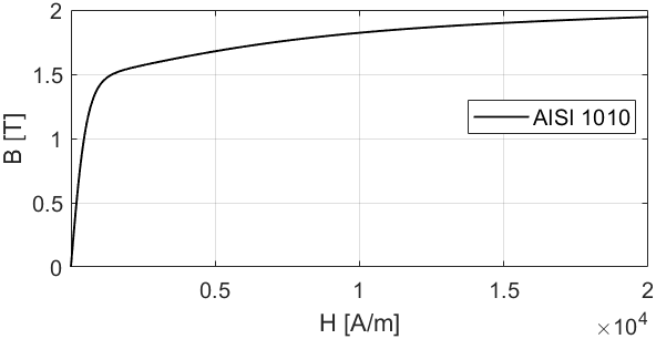
Having defined the above quantities, the task is now the estimation of iron and corresponding coil thickness such that the geometric and physical constraints specified in table 1, are fulfilled, after a certain choice for the iron material is made. As basic reference we consider a typical AISI 1010 $H$-$B$ curve, shown in figure 3.

Figure 3: Reference AISI 1010 $H$-$B$ curve.

Figure 4: Dependence of efficiency, maximum iron flux density, power, total current and maximum stray flux density, as a function of the yoke thickness $h$, as predicted by the model (3.1)–(3.3), (3.5)–(3.7).

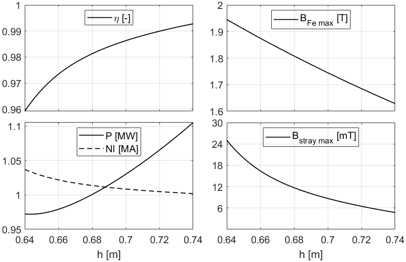
By solving eqs. (3.1)–(3.2) while assuming $h$ as parameter, one gets $t=y_{\text{max}}-b/2-h$, $B_{\text{Fe\,max}}=(c-t)(b+t)B/(2hc)$. In turn, eqs. (3.3), (3.5)–(3.7) and the mentioned $H$-$B$ curve we get $\eta$, $NI$, $P$ and $B_{\text{stray\,{max}}}$. The analysis has been carried out by assuming $B=1.25$ T, the geometrical parameters as described above, leading to the plots shown in figure 4.

From the inspection of the curves it is easily realized that the stray field decreases with increasing $h$. Conversely, the MMF shows weak variations with $h$ and tends toward its limit value (about 1 MA, eq. (3.5)). The power is evaluated by assuming the following values for copper resistivity $\rho=1.87\cdot 10^{-8}\>\Omega$ m (@ $T=42.5^{\circ}$C), and the filling factor, $f=0.65$, which is a reasonable value in the coil design. The corresponding curve shows a minimum for a specific value of the iron thickness, which provides a significant information to be exploited for the design. Minimising the stray field and the power at the same time results as conflicting goals.

Notice that one normally expects a completely different behaviour of the power, namely a reduction of $P$ when $NI$ gets reduced. In our case we have $P\propto 1/(\eta^{2}t)$, which is the product of a decreasing ($1/\eta^{2}$) and of an increasing ($1/t$) function of $h$, respectively. The result is a power function that has a minimum and then increases with $h$, instead of decreasing. This is due to the dimensional constraint (3.1), a specific peculiarity of the present design.

Within the considered model the $B_{\text{stray}}\leq 10\;$mT constraint is achieved with $h=0.7\;$m ($B_{\text{stray}}=8.7\;$mT), which yields to $\eta=0.986$, $P=1.03\;$MW, $\mathcal{F}=1.01\;$MA and $B_{\text{Fe\,max}}=1.74\;$T. However, it should be outlined that such quantities are highly sensitive to parameters variations. In particular, from eqs. (3.2), (3.7) the stray field sensitivity to variation of the yoke thickness $h$ can be expressed as

$$\frac{\mathrm{d}B_{\text{stray\,max}}/B_{\text{stray\,max}}}{\mathrm{d}h/h}=-\frac{c^{\prime}b^{\prime}+h^{2}}{(c^{\prime}+h)(b^{\prime}-h)}\frac{\mu_{\text{r}}(B_{\text{Fe\,max}})}{\mu_{\text{r\,diff}}(B_{\text{Fe\,max}})}\approx-10$$ (3.8)

where $c^{\prime}=c+\tfrac{b}{2}-y_{\text{max}}=6\>\text{m}$, $b^{\prime}=\tfrac{b}{2}+y_{\text{max}}=2.8\>\text{m}$, $\mu_{\text{r\,diff}}$ is the differential relative permeability and $h\approx 0.7$. The sensitivity resulting by considering different $H$-$B$ curves will be shown in next sections.

Finally it should be outlined that both copper and aluminum [11] were considered as materials for the conductor coil. However, since the limit in the coil size $t$ given by equation 3.1, the higher electrical resistivity of aluminium and the linear dependence of the power on $\rho$, a much larger dissipated power results from aluminum choice, which is not compatible with current CERN standards. For this reason, all the discussions carried out hereafter will refer to copper coils.

3.2 Integrated magnet design

This section describes the magnet design with due detail. It includes yoke, coil and thermal shield detailed design, with the main goal of trying to keep the ohmic power $P$ as low as possible while taking into account geometrical, electrical and thermal aspects. In particular: i) the yoke design accounting for specific iron magnetic properties; ii) the full electrical and cooling coil design, with constraints from integration of power supply according to CERN standards and iii) the integrated design of the thermal conditioning achieving the required temperature of the detector region. The due verification of the compatibility of such design option with mechanical loads, forces and stresses is treated in the following section 4.

3.2.1 Yoke

As stated in previous section, three geometrical parameters are specified by the design constraints, namely:

• total longitudinal magnet length $c=7.20$ m;

• horizontal gap $a=1.00$ m

• total height $2y_{\text{max}}=4.00$ m

The simplified analytical model shows (figure 4) that the limiting factor is the requirement to keep the stray field outside the magnet within the threshold $B_{\text{stray}}\leq 10$ mT specified in section 2, yielding a yoke thickness $h=0.70$ m.

Moreover, this choice for the yoke thickness provides a good magnet efficiency $\eta=0.986$ and a power $P=1.03$ MW, which is not far from the unconstrained minimum of $P=0.97$ MW. As for the geometrical parameters of the triangular septum $b_{\text{sept}}$ and $a_{\text{sept}}$ illustrated in figure 2 they are selected so as to minimize the interaction with the muons, whose distribution is depicted in figure 1a, as triangular septum height $b_{\text{sept}}=1.44$ m, and triangular septum width $a_{\text{sept}}=0.50$ m.

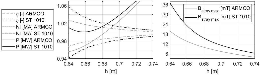
Some further considerations are due in terms of yoke material properties. Among yoke material types used at CERN there are, ordered by performances (and cost), low carbon steels, such as AISI 1010, special grade low carbon steels of relatively high purity, such as ARMCO${}^{\text{\textregistered}}$ grade 4, and cobalt iron. Ref. [14] reports $H$-$B$ curves of materials used as magnetic steel as they are obtained from measured samples, in particular different heats of 1010 steel and a special grade one. We consider their upper and lower bounds, that is the curves having the largest and lower $B$ strengths, which are labelled ARMCO ATLAS and ST 1010 ATLAS in ref. [14]. In the region of interest, corresponding to $B_{\text{Fe\,max}}=1.75$ T, the working point is identified by $H(B_{\text{Fe\,max}})=6.02$ kA/m and $H(B_{\text{Fe\,max}})=9.15$ kA/m for the two bounding materials, respectively.

Figure 5 shows the results obtained with the model (3.1)–(3.3), (3.5)–(3.7) and such bounds for iron characteristics. There is a clear evidence of the sensitivity with respect to the material. In particular, the variation of $P$ and $B_{\text{stray\,max}}$ is relevant in the region of interest. From now on we assume the ST1010 ATLAS as material for the yoke, being the most conservative choice. It is clear there is room for improvement by using better materials.

Figure 5: Dependence of efficiency, total current, power and maximum stray flux density, as a function of the yoke thickness $h$, as predicted by the model (3.1)–(3.3), (3.5)–(3.7), for yoke material curves corresponding to the considered upper and lower bounds, see text.

3.2.2 Coil

After the yoke has been determined in its size, shape and material we can afford the detailed design of the coil. It has to comply with the following additional constraints or criteria:

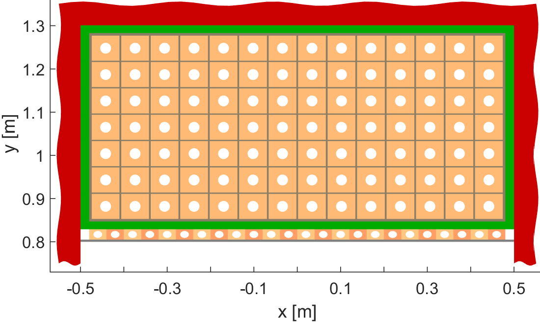
1. Coil cross-section. The total height of the magnetized volume $b=1.60$ m is specified (table 1). Therefore, the total thickness is $t=y_{\text{max}}-b/2-h=0.5$ m. However, the gross area $at$ is not fully available to the coil (see figure 6). The coil thickness $t_{\text{coil}}$ is less than $t$ to accommodate thermal shield, insulating laminates, mechanical supporting laminate in about 8 cm (figure 6c). Similarly, the coil width $a_{\text{coil}}$ is less than $a$, so as to leave about 4 cm of lateral space for the tie-rods that fix the coil to the iron and for thermal insulation  [14].

2. Winding type. A continuous double pancake coil configuration is assumed, so that all electrical and water pipe junctions are external to the magnet.

3. Voltage. The electric voltage $V$ at coil terminals should be as close as possible to 100 V so as to exploit synergy for power converters used at CERN.

4. Current. The electrical current $I$ should be less than 14.4 kA (so as to have no more than two standard 8 kA converter modules with a 10 % margin for control).

5. Cooling water temperature. The inlet temperature $T_{\text{in}}=(29\pm 1)$℃ is specified by the CERN EN-CV-INJ Department, whereas the outlet temperature $T_{\text{out}}$ should not exceed 60℃ to avoid damage to the resin.

6. Cooling water speed. To avoid erosion, corrosion and impingements, the speed $w$ should not exceed 3 m/s.

7. Reynolds number. To get a moderately turbulent flow, the condition $2000<\text{\emph{Re}}<10^{5}$ should be satisfied.

8. Pressure drop. In the water circuit, the pressure drop $\Delta p$ should not exceed the limit of 10 bar.

(a)
(b)
(c)	(d)

Figure 6: Cross-sections of the SND magnet: (a) in the plane $x=0$; (b) in the plane $z=0$, superimposed to the simulated muons flux distribution in the transverse plane immediately downstream of the last sweeper magnet [15]; (c) cut-out of the upper part in the plane $z=0$; (d) particular of the hollow bar type used as coil conductor. The gray box in (a–b) represents the instrumented region, where the mean flux density is specified as $B=1.25$ T.

The magnetomotive force $\mathcal{F}=NI$ of about 1 MA has been estimated in section 3.1 since, for the magnetic structure and materials considered, it mainly depends on the desired field $B$ and the horizontal gap size $a$. The effective cross-section of the coils and the value of the magnetomotive force are almost fixed by the above considerations. Therefore, as stated in section 3.1, the aluminum option is discarded in order to minimize the ohmic power $P$, which for a copper coil and a realistic filling factor $f=0.65$ is about 1 MW. The requirement of a total coil voltage $V$ of about 100 V leads to a current $I=P/V$ of about 10 kA, hence to a number of turns $N=\mathcal{F}/I$ of about 100. The opportunity to have cooling pipes of circular cross-section (hence coil turns of nearly square cross-section) and the ratio between $a_{\text{coil}}$ and $t_{\text{coil}}$, which is about 2, lead to select $N_{a}=14$ pancakes with $N_{b}=7$ turns each. That yields to $N=N_{a}N_{b}=98\approx 100$. It is worth noticing that:

• $N_{a}=14$, an even number, is compatible with the double pancake configuration;

• greater values of the number of turns, e.g. $N_{a}=16$ with $N_{b}=8$, would make the design of the cooling system more cumbersome and increase V above 100 V;

• the lower value of the number of turns $N=72$, with $N_{a}=12$ and $N_{b}=6$, still compatible with the constraint $I<14.4$ kA, would unnecessarily reduce the voltage well below 100 V, while increasing the cross-section of the single turns, which might yield problems when bending the conductor.

The next step is to specify the cross-section of the hollow bars, followed by the design of the cooling system. This design started from a first guess of the parameters and it went through a few iterations exploiting the results of more accurate numerical electrical and thermal analyses, as it will be shown in the next section. The selected design configuration is then reported in table 2 in comparison with the LHCb magnet. The 3-D analyses reported in the next section show that all constraints are satisfied. As expected, the value of the ohmic power $P=1.02$ MW is not far from the figure provided by the procedure based on lumped parameters. However, it is worth noticing that the ohmic power might further be optimized. Indeed, a significant reduction (about 10 %) can be obtained by relaxing the stray field limit to 15 mT, while selecting a different magnetic material and a variable thickness of the yoke (different values of top and side thickness).

Table 2: Reference design configuration of the detector and comparison with the main parameters of the LHCb magnet.

				SND	LHCb [7, 8, 9]
General magnet properties
	total power	$P$	[MW]	1.03	4.2
	magnet efficiency	$\eta$	[-]	.981
	internal usable space along $z$	$c_{i}$	[m]	5.43
	yoke thickness	$h$	[cm]	70
	max top stray field	$B_{\text{stray\,max}}$	[mT]	10
	max side stray field†		[mT]	9
	total iron mass		[t]	356	$\approx 1500$
Coil
	hollow bar material			Cu	Al-99.7
	n. of pancakes	$N_{a}$	[-]	14	$2\cdot 15$
	turns per pancake	$N_{b}$	[-]	7	15
	total turns	$N=N_{a}N_{b}$	[-]	98	$2\cdot 225$
	hollow bar width	$a_{\text{bar}}$	[mm]	64	50
	hollow bar height	$b_{\text{bar}}$	[mm]	58	50
	water hole diameter	$2r$	[mm]	25.5	25
	average turns length	$l_{t}$	[m]	16.6	19.3
	total winding length	$l_{\text{tot}}$	[km]	1.6	8.7
	total hollow bar mass	$m_{\text{tot}}$	[t]	46	$\approx 2\cdot 25$
	coil thickness	$t_{\text{coil}}$	[cm]	43.6
	total thickness	$t$	[cm]	50.1
	insulator/holes ratio	$S_{\text{i}}/(N\pi r^{2})$	[-]	1.12
	coil fill factor	$f_{\text{coil}}=S_{\text{active}}/(a_{\text{coil}}t_{\text{coil}})$	[-]	.75
	total fill factor	$f=S_{\text{active}}/(at)$	[-]	.62
Electrical and magnetic properties
	magnetomotive force	$\mathcal{F}=NI$	[MA]	1.014	$2\cdot 1.3$
	current per turn	$I$	[kA]	10.3	5.85 (6.6 max)
	voltage	$V$	[V]	99	730
	current density	$J$	[A/mm2]	3.2	2.9
	total resistance	$R$	[m$\Omega$]	9.6 @ 42.5 ∘C	130 @ 20 ∘C
	inductance	$L$	[H]	0.18	1.3
	stored magnetic energy	$W_{m}$	[MJ]	9.7	32
Double pancake configuration and cooling
	continuous bar length	$l_{\text{wc}}=2N_{b}l_{t}$	[m]	233	290‡
	parallel water circuits	$N_{\text{wc}}=N_{a}/2$	[-]	7
	inlet-outlet temperature raise	$\Delta T$	[∘C]	25	25
	total cooling flow	$q_{\text{tot}}$	[m3/h]	35	150
	water speed	$w$	[m/s]	2.7
	Reynolds number	Re/1000	[-]	98
	pressure drop	$\Delta p$	[bar]	6.8	11
† attained at $x=a/2$, $y=1.1$ m (see figure 10c)
‡ the LHCb magnet has a single pancake configuration

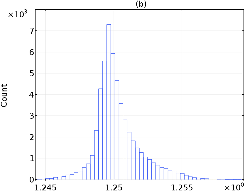
Finally in table 3 we compare main design figures calculated with the analytical model of section 3.1 and the accurate numerical model. Such comparison assumes iron ST 1010 ATLAS choice, a mean turns length $l_{t}=16.6$ m and a filling factor $f=0.62$ as accurately determined with the numerical model and reported in table 2. A very good agreement can be recognized.

Table 3: Comparison of the main design parameters from different modeling approaches.

		Analytical	FEM 3-D
$B$	[T]	1.25	1.25
$NI$	[MA]	1.01	1.014
${B}_{\text{Fe}}$	[T]	1.75	1.73
${B}_{\text{stray\,max}}$	[mT]	11	10

3.2.3 Thermal shield

 [^∘C]  

Figure 7: 2-D thermal numerical simulation for the reference configuration (table 2). The maximum temperature raise, $\Delta T=25^{\circ}$C, occurs between the outermost turns of odd and even pancakes. A differential thermal expansion of about 3 mm is calculated along the major magnet length $c$.

Figure 6c shows that the coil is thermally insulated. The proposed insulator is Vulkollan${}^{\text{\textregistered}}$ or a similar product, which has excellent mechanical properties, including elastic ones, to accommodate the different thermal expansion of the yoke. The inner and outer insulator thickness shown in green is taken as 18 mm, while the side one is 20 mm. The insulation layer plays also the role of reducing the temperature of the yoke, preventing magnetic ageing issues [14].

The additional single-layer copper circuit shown in the lower part of figure 6c, in contact with the inner coil insulation and with a supporting 5 mm thick non-magnetic steel laminate, is a thermal shield, hence not fed with any electric current, used to insulate the instrumented region, and keeps it at about $18\,^{\circ}$C. Such shield is made of copper hollow bars with rectangular cross-section with the following characteristics: two continuous even/odd parallel water circuits, each made of 12 turns and 181 m long, with corresponding inlet water pipes connected at opposite sides ($x\approx\pm 0.5$ m), to achieve a uniform temperature; total mass 2.3 t; input thermal power (from coil) about 6 kW; inlet/outlet water temperature 17/19 ^∘C; cross-section area $40\times 24$ mm²; elliptic cooling hole with major/minor diameter equal to 20/16 mm² and hydraulic diameter $d_{h}=17.7$ mm; water speed 1.56 m/s; Reynolds number about 38000; pressure drop 3.1 bar. The hydraulic diameter is given by four times the area divided by the perimeter of the (wetted) pipe cross-section. In the case of elliptic cross-section the perimeter can easily be calculated by means of standard special functions [19].

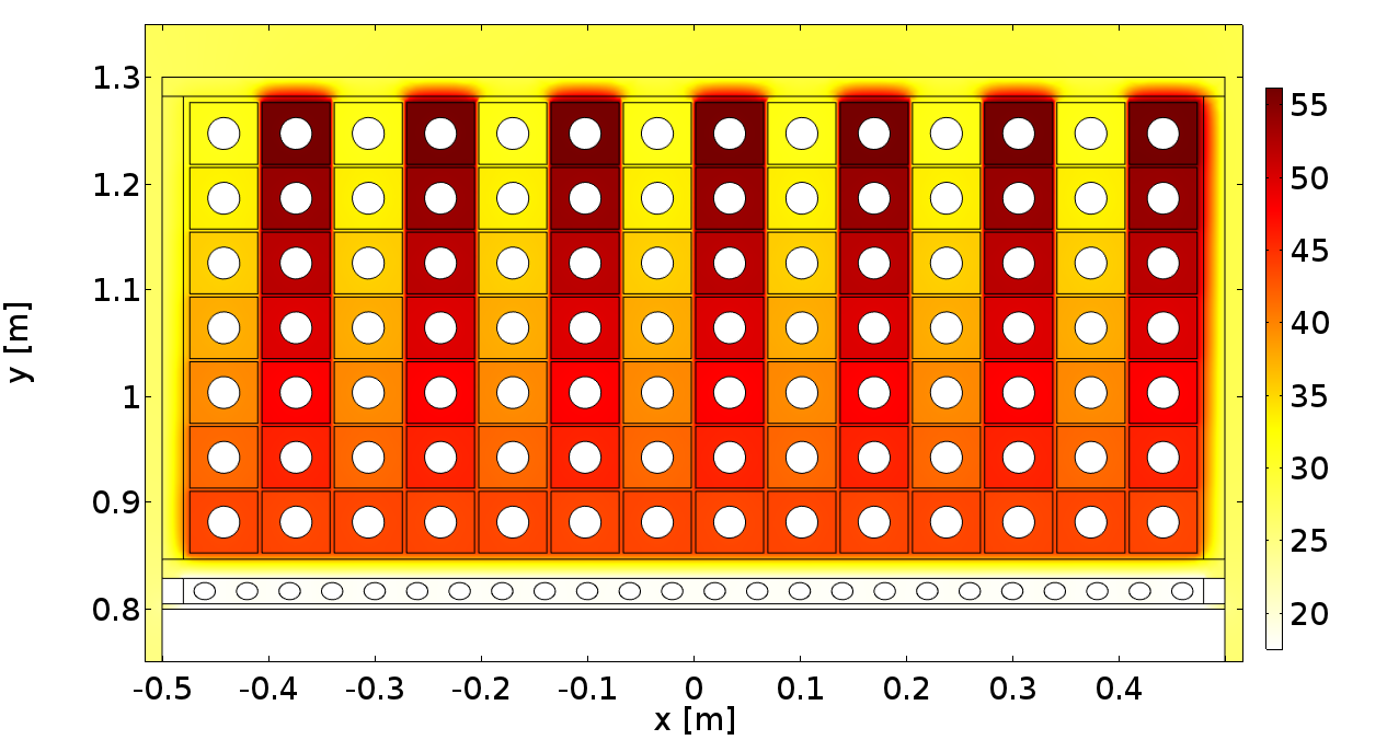
Figure 7 reports the result of a 2-D thermal numerical simulation for the design option of table 2. The double pancake configuration implies that the maximum temperature difference, $\Delta T=25\,^{\circ}$C, is attained between the outermost turns of odd and even pancakes. The consequent differential thermal expansion along the major magnet length, $c$, is about 3 mm. The resin encapsulating the coil will have to withstand such differential expansion.

3.3 3-D Field maps

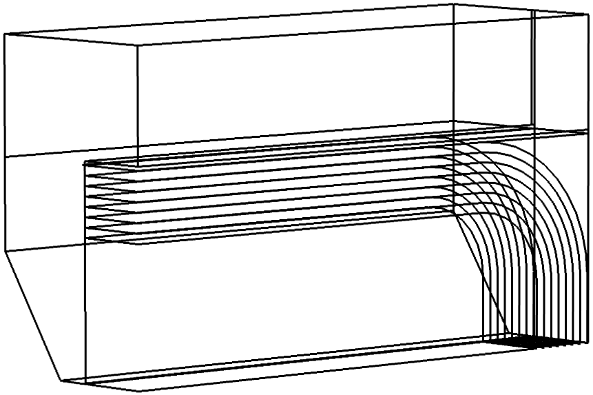
We report here the results of a detailed 3-D simulation of the electromagnetic problem, after the definition of the reference design as described in previous sections. Sizes and specifications are reported in table 2. In figure 8 the structure of the FEM model is sketched, with core and coil details. The magnetic curve ST 1010 ATLAS fit shown in figure 5 is assumed as reference iron model. Due to the symmetry only one eight of the entire structure is simulated, hereafter named block; on the corresponding cut boundaries the symmetry condition is imposed, as well as the magnetic insulation at the external region boundaries. Such block is meshed with a total of about 239000 nodes, of which about 102000 for the air gap region, 55000 for the iron yoke, 12600 for the coil and the remaining for the external region.

Figure 8: The 3-D model of the reference design

   [T]

Figure 9: $\lvert B\rvert$ mapping within the magnet and outside: 3-D view (left), 2-D section at $z=0$ (right). The point $(0,0,0)$ is the center of the magnet.

	[T]
	[mT]

Figure 10: (a) $B_{x}$ as a function of the horizontal axis $x$ at the $z=0$ section, for different horizontal lines at $y=0$, $y=0.3$, $y=0.6$, $y=0.75$ m. (b) Distribution of the $|B|$ values on the mesh points in the detector region. (c) $\lvert B_{\text{stray}}\rvert$ as a function of $x$ at the $z=0$ section, for different horizontal lines at $y=0$, $y=0.72$, $y=1.1$, $y=2.00$ m. (d) Stray field map $\sqrt{\smash[b]{B_{\text{stray}x}^{2}+B_{\text{stray}y}^{2}}}$ at the sections $z=\pm(c/2+2\>\text{cm})$, namely 2 cm upstream/downstream of the magnet.

Table 4: 3-D FEM analysis. Stray field at various $z=\text{constant}$ cross-sections and relevant yoke surface locations. $z=0$ and $z=2.7$ m correspond to the center and the end of the detector region (the gray box in figure 6a).

$xy$ yoke surface location				$z$	[m]	0	1.35	2.7
$@$ top	($x=0$, $y=y_{\text{max}}$)			$B_{\text{stray\,max}}$	[mT]	10	10	10
$@$ side	($x=a/2$, $y=1.10$ m)			$B_{\text{stray}}$	[mT]	9	8	7.5
$@$ septum	($x=1.00$ m, $y=0.43$ m)			$B_{\text{stray}}$	[mT]	5	5	4.5
$@$ max muons flux	($x=1.80$ m, $y=0$)			$B_{\text{stray}}$	[mT]	3	3	3

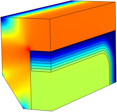
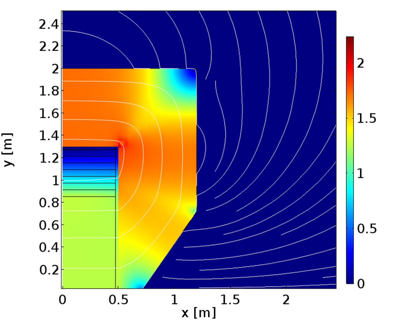
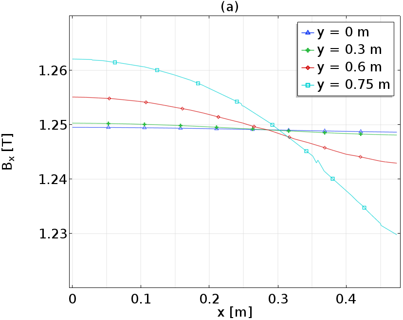
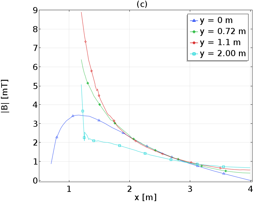
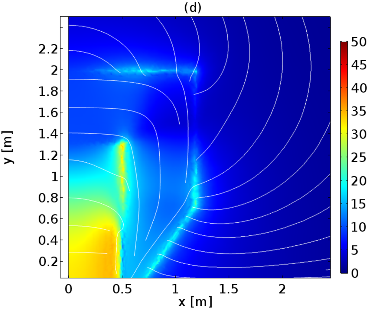
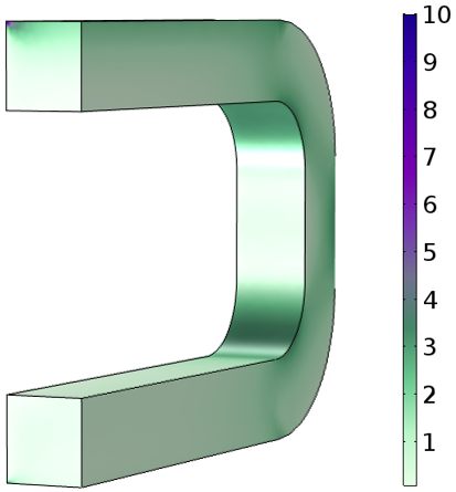
The FEM simulation for the set of used parameters is reported in figure 9, where the modulus of flux density $B$ is given in a 3-D view and 2-D section, respectively. The complete mapping of the field allows to evaluate the field uniformity within the detector region, and provide some local information at specified section/lines. Figure 10a reports the value of $B_{x}$ at the $z=0$ section for different horizontal lines. Figures 10 (a-b) show that the field uniformity $|\Delta B/B|$ in the internal region is limited to $\pm 1$ %, in agreement with the requirements. Figure 10c shows the external field $B_{\text{stray}}$ as a function of $x$ at the $z=0$ section for different horizontal lines, starting 1 mm away from the yoke. The line at $y=0$ starts at lower $x$ values because of the septum shape. The limit $B_{\text{stray\,max}}<10$ mT is fully accomplished as expected. Finally, in figure 10d a suggestive picture of the $\sqrt{\smash[b]{B_{\text{stray}x}^{2}+B_{\text{stray}y}^{2}}}$ field map is given at a vertical section immediately upstream of the magnet, 2 cm outside. Table 4 reports stray field values at relevant yoke surface locations.

4 Mechanical issues

4.1 Forces and stresses analysis

In order to complete the design, we have to consider the problem of the magnetic force and the corresponding induced stresses [16], due to Lorentz force on the coil that tend to burst the coil radially outward and crush it axially. In figure 11 a visual representation of such effects is given.

A fair evaluation of the total force can be obtained as that produced by an infinitely thin current sheet carrying the total current. In this way, following Maxwell’s stress tensor method [17], the magnetic force can easily be calculated by means of the magnetic pressure at the internal coil boundary as:

$$p_{\text{mag}}=\frac{B^{2}}{2\mu_{0}}.$$ (4.1)

where ${B}$ is the reference induction field within the chamber volume. This expression remains valid for the case of thick conductors, for which it can be thought as the difference at the inner and outer edges of the coil. Equation (4.1) consents to calculate the stress on the coil bent section, as well as the stresses on the straight sections transmitted to the iron, without dealing with the distributed body forces. Also the horizontal force pulling the vertical iron arms inward, and the corresponding induced stress, can be directly estimated by means of the magnetic pressure concept.

Figure 11: a) Magnetic coil self-force. b) Self-force stress at the coil edges. c) Iron stress induced by the coil vertical force. d) Horizontal magnetic force on the iron.

4.1.1 Analytical models

The evaluation of the coil stress at the bent edges is done by treating the coil as a thick-walled cylinder supporting the corresponding internal pressure of a gas. Using Lam equations [18], which give the stresses for thick-walled cylinders as a function of the radius $r$, and neglecting the external air pressure compared to the internal one, the tangential stress $\sigma_{t}$ is expressed as:

$$\sigma_{t}=p_{\text{mag}}\frac{r_{i}^{2}}{r_{e}^{2}-r_{i}^{2}}\biggl{(}1+\frac{r_{e}^{2}}{r^{2}}\biggr{)}$$ (4.2)

where $r_{i}=0.8$ m and $r_{e}=1.3$ m are the inner and outer coil radii, respectively.

The maximum tangential stress, that is the greatest magnitude of direct stress, amounts to 1 MPa, therefore well below the yield strength of the copper of about 50 MPa at $40^{\circ}$C. It has to be remarked that the real profile of the coil edge will slightly differ from the semi-cylindrical one in order to increase the inner volume available for the detectors. Nevertheless, the corresponding stresses are not expected to vary significantly. A more detailed analysis will be presented in section 4.1.2.

To evaluate the vertical force transmitted to the iron by the horizontal sections of the coil, the internal magnetic pressure has to be multiplied by the proper surface. The total resulting force on the upper part of the yoke will be the magnetic one reduced by the weights of the upper horizontal sections of both iron yoke and coil. Such force, equally distributed between the two vertical arms of the yoke, produces a maximum stress of about 1.5 MPa at the minimal iron thickness in the septum, that is well below the yield strength $\sigma_{\text{y}}=300$ MPa, which is the typical yield strength for standard iron.

The horizontal force pulling inward the vertical iron arms, and the corresponding induced stress, are also calculated via Maxwell’s stress tensor method. In this case the magnetic pressure (4.1) is pulling the vertical inner yoke surface because the magnetic field is nearly perpendicular in the air side. Then the bending moment is evaluated by assuming the vertical iron arm as a simply supported plate under bending where one dimensional model can be used, due to the typical ratio between the longitudinal $z$ and transversal $y$ dimension. The bending moment is then calculated with respect to a supported beam subject to the distributed horizontal load given by the magnetic pressure. Using the flexure formula, under the conservative assumption that the beam thickness coincides with the minimal section at the yoke septum, the maximum stress results in about 20 MPa, more than one order of magnitude below $\sigma_{\text{y}}$.

4.1.2 3-D analysis

The main mechanical stress on the structures is here analysed with 3-D FEM simulations. Sizes and specifications are reported in table 2.

Coupled magnetic-structural finite element 3-D analysis allows a more detailed assessment of the stresses due to the electromagnetic forces acting on both the coil and the iron yoke. In particular, the analysis returns the forces as distributed body loads overcoming the simplification of the magnetic pressure employed in the preliminary analysis. The coil has been modeled as a “racetrack” neglecting all the insulating layers whereas the iron yoke has been considered as a single piece. Note that, due to the presence of the floor, the bottom horizontal surface of the iron has been considered fixed along $y$. Therefore, for the mechanical case, the simulation cannot be restricted to 1/8 of the structure.

Figure 12a shows that the equivalent stress within the coil, evaluated according to the von Mises criterion, $\sigma_{\text{M}}$, reaches a maximum value of about 3.4 MPa in relatively small regions of the bent end. Compared to the analytic result, this is roughly a factor of 2 worse since the profile of the coil edge slightly differs from the semi-cylindrical one through a straight vertical section.

Figure 12b shows that the equivalent stress $\sigma_{\text{M}}$ within the iron yoke, reaches a value of about 8.3 MPa at the septum corresponding to the minimum iron section. This value is about one third of that previously estimated with the conservative assumption of considering for the whole vertical iron arm the minimum iron thickness of the septum.

[MPa]   [MPa]
(a)   (b)

Figure 12: The 3-D model of copper (a) and iron (b) stress

4.2 Some functional issues

We finally discuss some additional issues that, although not essential in the overall design as described above, are still relevant for more detailed design. It has to be recalled here that, beside the normal operation regime, the inner magnet volume as described in section 2 requires to be accessed for the detector installation and maintenance. Some opening mechanism needs to be defined, allowing reliable, simple and fast operations.

Different schemes can be considered, that are compatible with the presented design. The significant amount of work needed for their detailed exploration and comparison largely exceed the scope of this paper. Nevertheless we would like to show some possible solution here, accomplishing the requirements, giving some insight to the related mechanical issues. Such proposed segmentation and opening scheme is depicted in figure 13, where the iron yoke is split in independent parts, and a side opening is considered for each slab. The side slabs are coupled to the whole structure by means of dowels, and a undercarriage allows the lateral sliding. We consider in the following the problem of sizing the coupling dowels, the opening force due to residual iron magnetization and the possible deformation of the structure when a prescribed number of slabs is removed.

Figure 13: Overall structure of the SND magnet, with partial view of the internal detectors.

4.2.1 Structural dowels design

We tackle here the dimensioning of the dowels connecting the vertical iron arms to the upper and lower horizontal tracts of the yoke. They have to resist to the shear stress induced by the vertical force coming from the coil. The same assumptions (already considered in section 4.1.1) that the magnetic pressure internal to the chamber produces the force bursting the coil allow us to study the vertical force acting on the iron. Assuming that the magnetic pressure is uniform within the chamber, the force acting on the upper horizontal section of the iron yoke is evaluated as the product of pressure and surface. The total force will be the difference between the bursting force just calculated and the weights of the upper horizontal sections of both iron yoke and coil.

In order to find the dowel section able to withstand the vertical force acting on the iron we consider only the upper part of the iron yoke modeling the horizontal section as an isostatic beam. Therefore, the mobile part of the iron yoke has to balance the main force with a total constraint reaction of about 1740 kN. This reaction has to be sustained by dowels of proper cross-section. Assuming for the iron a $K_{t}$ (corrected yield strength) of 50 N/mm² (“low strength” iron), it is possible to find a total minimum surface of $35\cdot 10^{3}$ mm² needed for the whole dowels. For a 15 sections solution with the one dowel (see figure 13), 15 slabs, the diameter of the single dowel can be assumed to be 160 mm (including safety factors).

4.2.2 Opening force and deformations

The force required to open the magnet when the current is turned off (see section 2) can approximately be calculated as follows. Before opening the magnet, a current ramp down is performed, at the end of which the $B$ field pattern can be assumed to be qualitatively the same as the one corresponding to operation. The condition $I=0$ implies $aH+\ell H_{\text{Fe}}=NI=0$. Combining this equation with the flux balance equation  (3.2), while assuming $h\approx 0.7$ m, $t\approx 0.5$ m, $\ell\approx 3a$, provides $B_{\text{Fe}}=-\mu_{0}(c-t)(b+t)/(2hc)(\ell/a)H_{\text{Fe}}\approx-4\mu_{0}H_{\text{Fe}}$, which is a line in the second quadrant of the plane $(H_{\text{Fe}},B_{\text{Fe}})$. The worst-case condition is evaluated by assuming $H_{\text{Fe}}\approx H_{\text{c}}\approx 200$ A/m, where $H_{\text{c}}$ is the coercive field. That gives $B_{\text{Fe}}\approx 1$ mT, and in turn a force per unit surface $B_{\text{Fe}}^{2}/(2\mu_{0})\approx 0.5$ N/m², which is negligible.

Finally, as for reference, we calculated the worst case deformation of the structure when all the slabs are completely open, except for the two terminal ones, as shown in figure 13. The stress and deformation analyses for the open structure have been carried out with 3-D mechanical simulations, assuming an attachment boundary condition between the upper horizontal surface of the coil and the iron yoke. The maximum displacement for such case, attained at the top center of the structure on the opened face, is limited to about 30 $\mu m$, and the maximum Von Mises stress to about 6 MPa. Such values are fully compliant with admitted deformation of any involved structure and with the yield strength for both iron and copper.

The above analysis suggests no evident structural problem in the sectioning and opening scheme, at the considered detail level. The actual number of slabs as well as the opening scheme will be better specified and optimised in further design phases, according to specific requirements of the detector structure as well as to mechanical and manufacturing issues.

5 Conclusions

A realistic design of the magnet for the SND detector of the SHiP experiment, fully compliant with specifications and constraints has been provided. Different options have been preliminarily considered, defining the normal conducting copper solution as best suited to the problem for different order of reasons, from structural ones to resilience, reliability and maintenance.

Due to limitations in size and shape for the coil and yoke, the design task, basically played between the conflicting goals of high magnetic efficiency and minimal power consumption, revealed the need for some deepening of standard analytical design tools. The design optimization steps have been defined and described in detail, trying to give deep insight in the process.

Such developments have been the guidance for the 3-D FEM analysis, that has assessed the figures of merit and the general quality of the established design option. In particular a detailed design set of design parameters is given, fulfilling all the requirements and constraints.

Finally, beside the fundamental electromagnetic, thermal and mechanical analysis, some basic manufacturing issues related to the required accessibility of the SND along with realistic solutions have been described.

References

- [1] S. Alekhin et al., A facility to Search for Hidden Particles at the CERN SPS: the SHiP physics case, Rept. Prog. Phys. 79 (2016) 124201.
- [2] SHiP collaboration, A facility to Search for Hidden Particles (SHiP) at the CERN SPS, https://arxiv.org/abs/1504.04956.
- [3] C. Ahdida et al, The experimental facility for the Search for Hidden Particles at the CERN SPS, 2019 JINST 14 P03025.
- [4] SHiP collaboration, The active muon shield in the SHiP experiment, 2017 JINST 12 P05011.
- [5] OPERA collaboration, The OPERA experiment in the CERN to Gran Sasso neutrino beam, 2009 JINST 4 P04018.
- [6] C. Fukushima, M. Kimura, S. Ogawa, H. Shibuya, G. Takahashi (Toho U.), K. Kodama (Aichi U. of Education), T. Hara (Kobe U.), S. Mikado (Nihon U., Narashino), A thin emulsion spectrometer using a compact permanent magnet, 2008 Nucl. Instrum. Meth. A 592 56–62..
- [7] J. André, et al. Status of the LHCb magnet system, IEEE T. Appl. Supercond. 12.1 (2002): 366-371.
- [8] J. André, et al, Status of the LHCb dipole magnet, IEEE T. Appl. Supercond. 14.2 (2004): 509-513.
- [9] M. Losasso, et al, Tests and field map of LHCb dipole magnet, IEEE T. Appl. Supercond. 16.2 (2006): 1700-1703.
- [10] D. Tommasini, Private communication.
- [11] M. A. Green, Use of aluminum coils instead of copper coils in accelerator magnet systems, IEEE Trans. Nucl. Sci. 1967.
- [12] J. T. Tanabe, Iron Dominated Electromagnets: Design, Fabrication, Assembly And Measurements, World Scientific, 2005.
- [13] D. Tommasini, Practical Definitions and Formulae for Normal conducting Magnets, CERN internal Note 2011-18, Sep. 2011.
- [14] S. Sgobba, Physics and measurements of magnetic materials, CERN-2010-004, pp. 39-63, 2011.
- [15] SHiP Collaboration, SHiP experiment progress report, CERN-SPSC-2019-010; SPSC-SR-248, 2019.
- [16] D. B. Montgomery, Solenoid magnet design: the magnetic and mechanical aspects of resistive and superconducting systems, Wiley, 1969.
- [17] J. A. Stratton Electromagnetic Theory McGraw-Hill Book Company, Inc., 1941.
- [18] S. Timoshenko Strength of Materials Part II, Art. 70, D. Van Nostrand, Princeton, N.J., 1956
- [19] F. W. J. Olver, D. W. Lozier, R. F. Boisvert, C. W. Clark, NIST Handbook of Mathematical Functions, National Institute of Standards and Technology and Cambridge University Press, 2010. Online version: https://dlmf.nist.gov/