Transfer operator approach to ray-tracing in circular domains

Abstract

The computation of wave-energy distributions in the mid-to-high frequency regime can be reduced to ray-tracing calculations. Solving the ray-tracing problem in terms of an operator equation for the energy density leads to an inhomogeneous equation which involves a Perron-Frobenius operator defined on a suitable Sobolev space. Even for fairly simple geometries, let alone realistic scenarios such as typical boundary value problems in room acoustics or for mechanical vibrations, numerical approximations are necessary. Here we study the convergence of approximation schemes by rigorous methods. For circular billiards we prove that convergence of finite-rank approximations using a Fourier basis follows a power law where the power depends on the smoothness of the source distribution driving the system. The relevance of our studies for more general geometries is illustrated by numerical examples.

1 Introduction

Ray-tracing methods serve as an important toolkit in finding approximate solutions of linear wave equations in the high frequency limit. This approximation is used in a variety of fields providing, for example, the connection between Maxwell’s equations and geometric optics, as well as between quantum mechanics and classical Hamiltonian mechanics [13]. The ray-tracing limit has also been considered in detail in acoustics, seismology and mechanical vibrations [23]. In engineering applications, ray tracing is employed in handling electromagnetic problems, such as coverage estimates for 5G or WiFi communication [12], room acoustics simulations [22] as well as structure-borne sound propagation in mechanical structures [6]. Finding closed form, analytical solutions to such engineering problems of sufficient complexity is generally impossible, even using ray-tracing techniques, and one has to use numerical methods instead.

For solving linear wave problems such as those listed above, the numerical methods used have to be adapted to the relevant length and frequency scales involved. In the low frequency regime, finite element methods (FEM) are routinely employed for resolving the full wave dynamics. However, the number of degrees of freedom in an FEM model needs to scale with the wavelength and there is thus an upper limit in frequency above which the required computational resources become unfeasible. At very high frequencies, power balance approaches can often be used as long as certain assumptions on the ergodicity of the underlying ray dynamics are satisfied [24]. In the mid-to-high frequency range, ray-tracing becomes the method of choice; standard ray-tracing techniques track all possible rays from a source to a receiver point [22] — a method which becomes cumbersome if many reflections need to be taken into account. As an alternative Dynamical Energy Analysis (DEA) was proposed and has proven to be useful in particular for structure-borne sound problems [24, 14]. Instead of tracking individual rays carrying vibrations across the complex structure — which is extremely challenging — in DEA, the problem is reformulated in terms of densities of rays, which are then mapped across a mesh representing the structure [7, 8]. This reduces the ray tracing problem from tracking rays on complicated and curved domains to mapping ray segments across small, plane patches of a simple shape forming the mesh, typically triangular or quadrilateral mesh cells. The ray densities are then mapped from one cell of the mesh to adjacent ones and the overall transport problem can be formulated in terms of an inhomogeneous equation of the form

$$(I-\mathcal{L})f=f_{0}\,,$$ (1)

where $f_{0}$ is the initial ray density, $\mathcal{L}$ a Perron-Frobenius type operator describing the evolution of ray densities and $f$ the required final ray density. Using DEA, the distribution of vibrational energy in mechanical structures, such as ships, cars and tractors [15, 14] can be calculated successfully.

For such realistic geometries, equation (1) above cannot be solved analytically, so recourse is made to numerical schemes based on heuristic finite-dimensional matrix approximations of the operator $\mathcal{L}$. To date, very little is known about the convergence properties of these schemes and the dependence of the convergence rate on the ray dynamics, as well as the discretisation techniques [8]. The precise form of convergence is likely to be highly sensitive to both the basis functions used in approximating the inhomogeneous equation (1), as well as dynamical and damping properties of the system under investigation [15]. For our study, we will therefore be concerned with the approximation of $\mathcal{L}$ by operators of finite rank. There is a plethora of papers on numerical approximation of Perron-Frobenius operators, starting with Ulam’s method of phase space discretisation, finite section or Galerkin methods, and data-driven methods, see for example [2, 10, 11, 17, 19] to mention but a few. Surprisingly, the application of DEA (which falls into the Galerkin category) to even fairly simple geometries has not been dealt with at a rigorous level. Here, we shall thus focus on one of the simplest cases, the billiard dynamics given by the ballistic motion within a circular disk. We shall establish rigorous error bounds of finite-dimensional approximations for the resulting energy distribution.

In order to set up the required notation, consider a particle moving inside a circular billiard table $\cal{D}$ being specularly reflected at its boundary $\partial\cal{D}$. We parametrise $\partial\cal{D}$ by the polar angle $x\in\mathbb{R}/2\pi\mathbb{Z}$ and we denote by $y\in[-\pi/2,\pi/2]$ the angle of reflection that the postcollisional velocity vector has with the inward normal to $\partial\cal{D}$. Initially the collision angle is defined on an interval. It is, however, technically simpler to deal with cyclic variables. Since both angles $-\pi/2$ and $\pi/2$ correspond to a particle which sticks on the boundary we identify both angles so that the collision angle becomes a cyclic variable as well. With these conventions, the collision map $T$ on the domain $\Omega=(\mathbb{R}/2\pi\mathbb{Z})\times(\mathbb{R}/\pi\mathbb{Z})$ can be written as

$$T(x,y)=(x+\pi-2y,y),\quad\,(x,y)\in\Omega$$ (2)

with its inverse $\phi=T^{-1}$ given by

$$\phi(x,y)=(x-\pi+2y,y)\quad\,(x,y)\in\Omega\,.$$ (3)

It is not difficult to see that the collision map $T$ preserves the normalised Haar measure on $\Omega$. The long-term statistical behaviour of $T$ can thus be studied by investigating the associated Perron-Frobenius operator (see, for example, [5]), which for invertible measure-preserving maps is given by the composition operator $\mathcal{C}_{\phi}$ defined as

$$(\mathcal{C}_{\phi}f)(x,y)=f(\phi(x,y)),\quad(x,y)\in\Omega\,,$$ (4)

where $f\colon\Omega\to\mathbb{C}$. In the current work we are interested in the properties of a weighted Perron-Frobenius operator, also known as a transfer operator. In order to define it, let us first introduce a multiplication operator $\mathcal{M}_{w}$ acting on functions $f\colon\Omega\to\mathbb{C}$ by

$$(\mathcal{M}_{w}f)(x,y)=w(x,y)f(x,y),\quad(x,y)\in\Omega,$$ (5)

where $w\colon\Omega\to[0,\infty)$ is a suitable weight function, which in the DEA framework accounts for dissipation caused either by collisions with the wall or by in-flight dissipation. The transfer operator, understood to be acting on a suitable space of functions detailed in the following section, is now given by

$$\mathcal{L}=\mathcal{M}_{w}\mathcal{C}_{\phi}\,.$$ (6)

In the present article, we are interested in approximations of the solution to the operator equation (1) with $f_{0}\colon\Omega\to[0,\infty)$ interpreted as the initial boundary density of particles induced by the first boundary collision of particles emitted by a source located in the interior of $\cal{D}$ (see [24]). In the DEA approach this quantity represents the energy source. The resulting energy distribution is captured by the solution, $f\colon\Omega\to[0,\infty)$, which gives the stationary boundary density generated by the collision dynamics. Given a suitable Banach space and a sequence of finite-rank projections $(P_{K})_{K\in\mathbb{N}}$, an approximation method for (1) can be constructed by considering the projected finite-dimensional problem

$${\color[rgb]{0,0,0}(I-P_{K}\mathcal{L}P_{K})f_{K}=f_{0}\,.}$$ (7)

The aim of this work is to present a Banach space for $f_{0}$ and $(P_{K})_{K\in\mathbb{N}}$, so that problem (7) has solutions, which converge in a suitable topology to the solution of (1) as $K$ tends to infinity, with the speed of convergence being of the order $K^{-\alpha}$. The exponent $\alpha$ depends on the smoothness of $f_{0}$ and the requirements imposed on the type of convergence.

In passing we note that transfer operators have their roots in statistical mechanics [20, 21] and nowadays play an important role in the ergodic theory of smooth expanding, or more generally, hyperbolic dynamical systems (see, for example, [3, 4]). The main reason for their popularity in this context derives from the fact that for expanding or hyperbolic dynamical systems the transfer operator, when considered on a suitable function space, can be shown to have discrete peripheral spectrum, from which long-term statistical properties of the underlying system can be derived. In the elliptic setting, however, such as for the circular billiard considered in this article, analogous results cannot be expected, and, as a consequence, transfer operator methods have received little attention in this context. It is perhaps worth noting that in our setting we do not require discreteness of the peripheral spectrum of the transfer operator. The main onus is to show that the resolvent of the transfer operator exists at the point $1$ (see equation (1)) and can be effectively approximated by finite-rank operators (see equation (7)).

As we intend to keep our presentation accessible to non-specialists, we will occasionally elaborate on aspects covered in the specialised literature but which may not be well known to a general audience. The remaining parts are organised as follows. In Section 2 we introduce Sobolev spaces, on which the transfer operator and its finite-dimensional approximations are bounded operators with spectral radii bounded away from $1$. In Section 3 we shall prove the convergence results for the operator equations (1) and (7) stated as Theorem 3.4. In the final Section 4 we summarise the main findings, compare the formal results with numerical simulations and explore the relevance of the current study in a wider context.

2 Sobolev spaces and transfer operators

We will be interested in certain subspaces of $L^{2}(\Omega)=L^{2}(\Omega,m)$ where $dm=dxdy/(2\pi^{2})$ is the normalised two-dimensional Lebesgue measure on $\Omega$. The natural inner product is given by

$$(f,g)_{L^{2}}=\int_{\Omega}f(x,y)\overline{g(x,y)}{\rm d}m\,.$$

An orthonormal basis of $L^{2}(\Omega)$ is given by $\{e_{k}\colon k\in\mathbb{Z}^{2}\}$ where $e_{k}(x,y)=\mathrm{e}^{\mathrm{i}k_{1}x}\mathrm{e}^{2\mathrm{i}k_{2}y}$ so that $f(x,y)=\sum_{k\in\mathbb{Z}^{2}}c_{k}(f)e_{k}(x,y)$ with Fourier coefficients $c_{k}(f)=(f,e_{k})_{L_{2}}$.

Definition 2.1.

Let $m=(m_{1},m_{2})\in\mathbb{N}_{0}^{2}$. The Sobolev space $H^{m}(\Omega)$ is the collection of all $f\in L^{2}(\Omega)$ such that for all $\nu=(\nu_{1},\nu_{2})\in\mathbb{N}^{2}$ with $\nu_{1}\leq m_{1}$ and $\nu_{2}\leq m_{2}$ the weak derivatives $D^{\nu}f=D_{x}^{\nu_{1}}D_{y}^{\nu_{2}}f$ exist and belong to $L^{2}(\Omega)$.

The space $H^{m}(\Omega)$ is a Hilbert space, when equipped with the inner product

$$(f,g)_{H^{m}}=(f,g)_{L^{2}}+(D^{m_{1}}_{x}f,D^{m_{1}}_{x}g)_{L^{2}}+(D^{m_{2}}_{y}f,D^{m_{2}}_{y}g)_{L^{2}}\,.$$ (8)

One can rewrite this definition in terms of Fourier coefficients. Using the fact that $c_{k}(D^{\nu}f)=(\mathrm{i}k_{1})^{\nu_{1}}(2\mathrm{i}k_{2})^{\nu_{2}}c_{k}(f)$, equation (8) can be expressed as

$$(f,g)_{H^{m}}=\sum_{k\in\mathbb{Z}^{2}}(1+|k_{1}|^{2m_{1}}+|2k_{2}|^{2m_{2}})c_{k}(f)\overline{c_{k}(g)}\,.$$ (9)

Remark 2.2.

For $m=(m_{1},m_{2})$ with $m_{1}=m_{2}$ the Sobolev space $H^{m}(\Omega)$ coincides with the classical isotropic Sobolev space, while for $m_{1}\neq m_{2}$, the space is an example of an anisotropic Sobolev space (see, for example, [9, Sec. 2.2]).

Using equation (9) we can define fractional Sobolev spaces $H^{s}(\Omega)$ for $s=(s_{1},s_{2})\in\mathbb{R}^{2}_{+}$ as

$$H^{s}(\Omega)=\left\{f\in L^{2}(\Omega)\colon\sum_{k\in\mathbb{Z}^{2}}|c_{k}(f)|^{2}(1+|k_{1}|^{2s_{1}}+|2k_{2}|^{2s_{2}})<\infty\right\},$$

which are Hilbert spaces when equipped with the inner product given in equation (9) with $m$ replaced by $s$.

We shall next investigate the properties of the composition operator $\mathcal{C}_{\phi}$ associated with the map $\phi$ in (3) on the fractional Sobolev space $H^{s}(\Omega)$.

Lemma 2.3.

The composition operator $\mathcal{C}_{\phi}$ given in (4) considered on $H^{s}(\Omega)$ with $s_{1}\geq s_{2}\geq 0$ is bounded, with spectral radius $r(\mathcal{C}_{\phi})=1$.

Proof.

For any $n\in\mathbb{N}$ and $(x,y)\in\Omega$ we have $\phi^{n}(x,y)=(x-n\pi+2ny,y)$, and thus

$$(\mathcal{C}^{n}_{\phi}e_{k})(x,y)=(\mathcal{C}_{\phi^{n}}e_{k})(x,y)=(-1)^{k_{1}n}e_{k_{1},nk_{1}+k_{2}}(x,y),$$ (10)

for any $k\in\mathbb{Z}^{2}$.

In order to show that the operator is bounded we will need the following general inequality. Let $(x,y)\in[0,\infty)^{2}$ and $t\geq 0$, then

$$(x+y)^{t}\leq C_{t}(x^{t}+y^{t}),\quad\mbox{ with }C_{t}=\max(1,2^{t-1}).$$ (11)

Using equation (11) we obtain the bound $|nk_{1}+k_{2}|^{2s_{2}}\leq C_{2s_{2}}(n^{2s_{2}}|k_{1}|^{2s_{1}}+|k_{2}|^{2s_{2}})$ for $s_{1}\geq s_{2}$, which leads to

$$\|\mathcal{C}^{n}_{\phi}e_{k}\|_{H^{s}}^{2}=1+|k_{1}|^{2s_{1}}+|2(nk_{1}+k_{2})|^{2s_{2}}\leq\left(1+C_{2s_{2}}(2n)^{2s_{2}}\right)\|e_{k}\|^{2}_{H^{s}}.$$

Since $(\mathcal{C}^{n}_{\phi}e_{k},\mathcal{C}^{n}_{\phi}e_{l})_{H^{s}}=0$ for $k\neq l$, the operator norm of $\mathcal{C}^{n}_{\phi}$ is bounded from above by $\left(1+(2n)^{2s_{2}}\max(1,2^{2s_{2}-1})\right)^{1/2}$, resulting in the upper bound for the spectral radius

$$r(\mathcal{C}_{\phi})=\lim_{n\to\infty}\|\mathcal{C}^{n}_{\phi}\|^{1/n}\leq\lim_{n\to\infty}\left(1+(2n)^{2s_{2}}\max(1,2^{2s_{2}-1})\right)^{1/(2n)}=1\,.$$

In order to see that the inequality above is an equality, observe that the operator norm of $\mathcal{C}^{n}_{\phi}$ is bounded from below by $1$ as $\|\mathcal{C}^{n}_{\phi}e_{0}\|_{H^{s}}=\|e_{0}\|_{H^{2}}$. Thus $r(\mathcal{C}_{\phi})=1$. ∎

Before proceeding we note that by (10), the action of the composition operator on $H^{s}(\Omega)$ can be represented by the action of the matrix

$$A=\begin{pmatrix}1&0\\ 1&1\end{pmatrix}$$

on Fourier coefficients. In particular, we have

$$\mathcal{C}^{n}_{\phi}e_{k}=(-1)^{k_{1}n}e_{A^{n}k}.$$ (12)

For $K\in\mathbb{N}$ define $\Lambda_{K}=\Lambda_{K}^{0}=\{(k_{1},k_{2})\in\mathbb{Z}^{2}\colon|k_{1}|<K,|k_{2}|<K\}$, and let $\Lambda_{K}^{n}=A^{n}(\Lambda_{K})$. Then for any $n\in\mathbb{N}_{0}$ we can define a finite-rank operator $P_{\Lambda_{K}^{n}}\colon H^{s}(\Omega)\to H^{s}(\Omega)$ by

$$(P_{\Lambda^{n}_{K}}f)(x,y)=\sum_{k\in\Lambda^{n}_{K}}c_{k}(f)e_{k}(x,y),\quad(x,y)\in\Omega\,.$$ (13)

Lemma 2.4.

Let $\mathcal{C}_{\phi}$ and $P_{\Lambda_{K}}$ be as above. Then

$$\mathcal{C}^{n}_{\phi}P_{\Lambda_{K}}=P_{\Lambda^{n}_{K}}\mathcal{C}^{n}_{\phi}$$

for any $n,K\in\mathbb{N}_{0}$.

Proof.

This follows by checking the equality for any basis element $e_{k}$ and noting that $A^{n}$ is invertible. ∎

Definition 2.5.

Let $\mathcal{M}_{w}$ denote the multiplication operator as defined in equation (5), considered as an operator on $H^{s}(\Omega)$, with a smooth weight function $w\colon\Omega\to[0,\infty)$. In addition, we assume that $w$ has the following properties:

1. $\|w\|_{\infty}=\sup_{x\in\Omega}|w(x)|<1$;

2. $w$ is bounded away from zero;

3. $w(x,y)=w(x^{\prime},y)$ for any $(x,y),(x^{\prime},y)\in\Omega$, that is, the weight $w$ does not depend on the first argument.

Remark 2.6.

The operator $\mathcal{M}_{w}$ models the effect of damping on the motion of the billiard particle. Assumptions (a) and (b) imply that the damping is well-behaved, while assumption (c) is innocuous, given the circular symmetry of the billiard table.

The following two lemmas summarise basic properties of $\mathcal{M}_{w}$ and $\mathcal{C}_{\phi}$.

Lemma 2.7.

Let $\mathcal{M}_{w},\mathcal{C}_{\phi}$ and $P_{\Lambda_{K}}$ be as above. Then we have the following.

1. $\mathcal{M}_{w}\mathcal{C}_{\phi}=\mathcal{C}_{\phi}\mathcal{M}_{w}$;

2. $D_{x}\mathcal{C}_{\phi}=\mathcal{C}_{\phi}D_{x}$;

3. $D_{x}\mathcal{M}_{w}=\mathcal{M}_{w}D_{x}$;

4. $D_{y}\mathcal{C}^{n}_{\phi}=2n\mathcal{C}^{n}_{\phi}D_{x}+\mathcal{C}^{n}_{\phi}D_{y}$ for $n\in\mathbb{N}$;

5. $D_{y}\mathcal{M}_{w}^{n}=n\mathcal{M}_{w}^{n-1}\mathcal{M}_{D_{y}w}+\mathcal{M}_{w}^{n}D_{y}$ for $n\in\mathbb{N}$;

6. $D_{x}P_{\Lambda_{K}}=P_{\Lambda_{K}}D_{x}$ and $D_{y}P_{\Lambda_{K}}=P_{\Lambda_{K}}D_{y}$ for $K\in\mathbb{N}$.

Proof.

Items (i) and (iii) follow from Definition 2.5(c); items (ii) and (iv) follow by direct computation using the map $\phi$; item (v) is obvious and (vi) is a direct consequence of the relations $c_{k}(D_{x}f)=(\mathrm{i}k_{1})c_{k}(f)$ and $c_{k}(D_{y}f)=(2\mathrm{i}k_{2})c_{k}(f)$. ∎

We write $\mathcal{L}_{K}=P_{\Lambda_{K}}\mathcal{M}_{w}\mathcal{C}_{\phi}P_{\Lambda_{K}}$ for the finite-rank approximation of $\mathcal{L}=\mathcal{M}_{w}\mathcal{C}_{\phi}$. Using Lemma 2.7 (i) and Lemma 2.4, we can write $\mathcal{L}_{K}^{n}$ for $n\in\mathbb{N}$ as

$$\mathcal{L}^{n}_{K}=(P_{\Lambda_{K}}\mathcal{M}_{w}\mathcal{C}_{\phi}P_{\Lambda_{K}})^{n}=P_{\Lambda_{K}}\left(\prod_{l=1}^{n}\mathcal{M}_{w}P_{\Lambda^{l}_{K}}\right)\mathcal{C}^{n}_{\phi}.$$ (14)

In order to state the properties of $\mathcal{L}$ and $\mathcal{L}_{K}$ we need to introduce the following multi-index notation: an $n$-dimensional multi-index is an $n$-tuple $\boldsymbol{i}_{n}=(i_{1},i_{2},\ldots,i_{n})$ of non-negative integers of order $|\boldsymbol{i_{n}}|=i_{1}+i_{2}+\cdots+i_{n}=m$; the corresponding multinomial coefficient is given by

$$\binom{m}{\boldsymbol{i}_{n}}=\frac{m!}{i_{1}!i_{2}!\cdots i_{n}!}\,.$$

Lemma 2.8.

Let $\mathcal{M}_{w},\mathcal{C}_{\phi}$ and $P_{\Lambda^{l}_{K}}$ be as above. Then we have the following.

1. $D_{y}^{m}\mathcal{C}_{\phi}=\sum_{i=0}^{m}2^{m-i}\binom{m}{i}\mathcal{C}_{\phi}D_{x}^{m-i}D_{y}^{i}$;

2. $D_{y}^{m}\mathcal{C}_{\phi}^{n}=\sum_{|\boldsymbol{i}_{n+1}|=m}2^{m-i_{n+1}}\binom{m}{\boldsymbol{i}_{n+1}}\mathcal{C}_{\phi}^{n}D_{x}^{m-i_{n+1}}D_{y}^{i_{n+1}}$;

3. $D_{y}^{m}\left(\prod_{l=1}^{n}\mathcal{M}_{w}P_{\Lambda^{l}_{K}}\right)=\sum_{|\boldsymbol{i}_{n+1}|=m}\binom{m}{\boldsymbol{i}_{n+1}}\left(\prod_{l=1}^{n}\mathcal{M}_{D^{i_{l}}_{y}w}P_{\Lambda^{l}_{K}}\right)D_{y}^{i_{n+1}}$.

Proof.

Item (i) follows by induction over $m$ using Lemma 2.7(iv) for the base case $m=1$. For item (ii), the additional induction over $n$ follows by rewriting (i) as $D_{y}^{m}\mathcal{C}_{\phi}=\sum_{i_{1}+i_{2}=m}2^{i_{1}}\binom{m}{i_{1},i_{2}}\mathcal{C}_{\phi}D^{i_{1}}_{x}D_{y}^{i_{2}}$. Finally, item (iii) follows from the Leibniz formula. ∎

We are now ready to prove the main result of this section. Keeping in mind that we assume that the billiard dynamics is dissipative, that is, the weight is chosen so that $\|w\|_{\infty}<1$, the following lemma shows that, given $f_{0}\in H^{s}(\Omega)$, the problem (1) and the projected version (7) have unique solutions $f\in H^{s}(\Omega)$ and $f_{K}\in H^{s}(\Omega)$, respectively.

Lemma 2.9.

Consider $\mathcal{L}$ and $\mathcal{L}_{K}$, $K\in\mathbb{N}$, as operators on $H^{s}(\Omega)$ for $s\in\mathbb{N}_{0}^{2}$ with $s_{1}\geq s_{2}\geq 0$. Then

1. $(\mathcal{L}_{K})_{K\in\mathbb{N}}$ is a family of bounded operators $H^{s}(\Omega)$ with norms bounded uniformly in $K$. Moreover, $r(\mathcal{L}_{K})\leq\|w\|_{\infty}$ for all $K$;

2. $\mathcal{L}$ is a bounded operator on $H^{s}(\Omega)$ with $r(\mathcal{L})\leq\|w\|_{\infty}$.

Proof.

We shall only prove statement (i), as the proof of statement (ii) follows by almost identical arguments. In the following, we shall assume that $s_{1}\geq s_{2}\geq 1$, as the case $s_{1}s_{2}=0$ follows by identical arguments. For $f\in H^{s}(\Omega)$ we have

$$\|\mathcal{L}^{n}_{K}f\|^{2}_{H^{s}}=\|\mathcal{L}^{n}_{K}f\|^{2}_{L^{2}}+||D^{s_{1}}_{x}\mathcal{L}^{n}_{K}f\|^{2}_{L^{2}}+\|D^{s_{2}}_{y}\mathcal{L}^{n}_{K}f\|^{2}_{L^{2}}\,.$$ (15)

Let $p,q\in\mathbb{N}$ with $p\leq s_{1}$ and $q\leq s_{2}$. It is not difficult to see that for any $f\in H^{s}(\Omega)$ and $K\in\mathbb{N}_{0}$ the following holds.

1. $\|P_{\Lambda_{K}^{j}}f\|_{L^{2}}\leq\|f\|_{L^{2}}$ for any $j\in\mathbb{N}_{0}$;

2. $\|\mathcal{M}_{w}f\|_{L^{2}}\leq\|w\|_{\infty}\|f\|_{L^{2}}$;

3. $\|D^{p}_{x}f\|^{2}_{L^{2}}\leq\|D^{s_{1}}_{x}f\|^{2}_{L^{2}}$ and $\|D^{q}_{x}f\|^{2}_{L^{2}}\leq\|D^{s_{2}}_{x}f\|^{2}_{L^{2}}$;

4. $\|D^{p}_{x}D^{q}_{y}f\|^{2}_{L^{2}}\leq\|D^{p+q}_{x}f\|^{2}_{L^{2}}+\|D^{p+q}_{y}f\|^{2}_{L^{2}}$ wherever $p+q\leq s_{2}$.

Here, statements (c) and (d) follow by writing the $L^{2}$ norm of $D_{x}^{p}f$ and $D_{y}^{q}f$ using Parseval’s identity.

Writing $\mathcal{L}^{n}_{K}$ as in equation (14) and using (a) and (b) above iteratively we have

$$\|\mathcal{L}^{n}_{K}f\|_{L^{2}}=\|(P_{\Lambda_{K}}\mathcal{M}_{w}\mathcal{C}_{\phi}P_{\Lambda_{K}})^{n}f\|_{L^{2}}\leq\|w\|^{n}_{\infty}\|\mathcal{C}^{n}_{\phi}f\|_{L^{2}}\leq\|w\|^{n}_{\infty}\|f\|_{L^{2}},$$ (16)

where the last inequality follows from the fact that the operator norm of $\mathcal{C}_{\phi}$ on $L^{2}(\Omega)$ equals $1$.

As $D_{x}$ commutes with any of the operators involved (Lemma 2.7 (ii,iii,vi)) we have in the second term on the right-hand side of (15) that $D^{s_{1}}_{x}\mathcal{L}_{K}^{n}=\mathcal{L}_{K}^{n}D^{s_{1}}_{x}$. By the same argument as above we have

$$\|D^{s_{1}}_{x}\mathcal{L}^{n}_{K}f\|_{L^{2}}\leq\|w\|^{n}_{\infty}\|D^{s_{1}}_{x}f\|_{L^{2}}.$$ (17)

In order to bound the last term in equation (15) we are using Lemma 2.8(iii) and Hölder’s inequality in order to write

$$\|D_{y}^{s_{2}}\mathcal{L}_{K}^{n}f\|_{L^{2}}^{2}=\|\sum_{j=0}^{s_{2}}A_{j}D^{j}_{y}\mathcal{C}_{\phi}^{n}f\|^{2}_{L^{2}}\leq(s_{2}+1)\sum_{j=0}^{s_{2}}\|A_{j}\|^{2}_{L^{2}}\|D^{j}_{y}\mathcal{C}_{\phi}^{n}f\|^{2}_{L^{2}},$$

where $A_{j}=\sum_{|\boldsymbol{i}_{n}|=s_{2}-j}\binom{s_{2}}{\boldsymbol{i}_{n},j}\left(\prod_{l=1}^{n}M_{D^{i_{l}}_{y}w}P_{\Lambda^{l}_{K}}\right)$.

We shall first obtain a bound for $\|D^{j}_{y}\mathcal{C}_{\phi}^{n}f\|_{L^{2}}$. Using Lemma 2.8(ii) and decomposing the sum in terms of powers of $D_{x}$ and $D_{y}$ we obtain

$$D^{j}_{y}\mathcal{C}_{\phi}^{n}=(2n)^{j}C_{\phi}^{n}D_{x}^{j}+C_{\phi}^{n}D_{y}^{j}+\sum_{|\boldsymbol{i}_{n+1}|=j\atop 0<i_{n+1}<j}2^{j-i_{n+1}}\binom{j}{\boldsymbol{i}_{n+1}}\mathcal{C}_{\phi}^{n}D_{x}^{j-i_{n+1}}D_{y}^{i_{n+1}},$$

where we have used the multinomial formula $\sum_{|\boldsymbol{i}_{n}|=k}\binom{k}{\boldsymbol{i}_{n}}=n^{k}$. Thus, for $j\leq m$ we obtain using Hölder’s inequality, the multinomial formula and upper bounds for $2^{j-i_{n+1}}$

$$\|D^{j}_{y}\mathcal{C}_{\phi}^{n}f\|^{2}_{L^{2}} \leq 2^{j}(n+1)^{j}\left(2^{j}n^{j}\|D_{x}^{j}f\|^{2}_{L^{2}}+\|D_{y}^{j}f\|^{2}_{L^{2}}\right)$$ (18)

$$+2^{j}(n+1)^{j}\left((2^{j}(n+1)^{j}-2^{j}n^{j}-1)\max_{0<i<j}\|D_{x}^{j-i}D_{y}^{i}f\|^{2}_{L^{2}}\right)$$

$$\leq 2^{2s_{2}}(n+1)^{2s_{2}}\left(\|D_{x}^{s_{1}}f\|^{2}_{L^{2}}+\|D_{y}^{s_{2}}f\|^{2}_{L^{2}}\right),$$

where the last inequality uses (c) and (d).

Next we shall obtain a bound on the operator norm of $A_{j}$ for $j\leq s_{2}$. First note that $\mathcal{M}_{D_{y}^{l}w}=\mathcal{M}_{w}\mathcal{M}_{(D_{y}^{l}w)/w}$ is well-defined as $w$ is bounded away from zero. By using (a) and (b) iteratively, for any $\boldsymbol{i}_{n}=(i_{1},\ldots,i_{n})$ with $|\boldsymbol{i}_{n}|=s_{2}$ we have

$$\|\prod_{l=1}^{n}\mathcal{M}_{D^{i_{l}}_{y}w}P_{\Lambda^{l}_{K}}f\|^{2}_{L^{2}}\leq C_{s_{2}}\|w\|^{2n}_{\infty}\|f\|^{2}_{L^{2}}$$

where $C_{s_{2}}=\max_{i_{1},\ldots,i_{n}\atop|\boldsymbol{i}_{n}|=s_{2}}\left(\prod_{l=1}^{n}\|D^{i_{l}}_{y}w/w\|^{2}_{\infty}\right)\leq\max_{0\leq l\leq s_{2}}\|D^{l}_{y}w/w\|_{\infty}^{2s_{2}}$ is a constant independent of $n$. Using arguments analogous to those used to obtain inequality (18), we obtain the bound

$$\|A_{j}\|_{L^{2}}^{2}\leq(n+1)^{2s_{2}}C_{s_{2}}\|w\|_{\infty}^{2n}\,.$$ (19)

Using the estimates (16), (17), (18) and (19) in equation (15) we arrive at the bound

$$\|\mathcal{L}^{n}_{K}f\|^{2}_{H^{s}}\leq\tilde{C}_{n,s_{2}}\|w\|_{\infty}^{2n}\|f\|^{2}_{H^{2}}\,$$

with $\tilde{C}_{n,s_{2}}\leq(s_{2}+1)s_{2}(n+1)^{4s_{2}}2^{2s_{2}}C_{s_{2}}+1$. As $\tilde{C}_{n,s_{2}}$ is independent of $K$, the family $(\mathcal{L}_{K})_{K\in\mathbb{N}}$ is a uniformly bounded family of bounded operators on $H^{s}(\Omega)$. Finally, taking the right hand side of equation (15) to the power of $1/n$ and observing that $\tilde{C}_{n,s_{2}}$ grows polynomially in $n$, the upper bound for the spectral radius of $\mathcal{L}_{K}$ follows. ∎

3 Convergence properties

In the previous section we established (see Lemma 2.9) that given $f_{0}\in H^{s}(\Omega)$, the problem (1) and the projected version (7) have unique solutions $f\in H^{s}(\Omega)$ and $f_{K}\in H^{s}(\Omega)$, respectively. We shall now turn to establishing the convergence of $f_{K}$ to $f$. This would be straightforward if we knew that $\mathcal{L}_{K}\to\mathcal{L}$ as $K\to\infty$ in the operator norm on $H^{s}(\Omega)$, since then, using the so-called second resolvent identity

$$(I-\mathcal{L})^{-1}-(I-\mathcal{L}_{K})^{-1}=-(I-\mathcal{L})^{-1}(\mathcal{L}-\mathcal{L}_{K})(I-\mathcal{L}_{K})^{-1}\,,$$ (20)

we would have

$$\|f-f_{K}\|_{H^{s}}=\|(I-\mathcal{L})^{-1}f_{0}-(I-\mathcal{L}_{K})^{-1}f_{0}\|_{H^{s}}=\|(I-\mathcal{L})^{-1}(\mathcal{L}_{K}-\mathcal{L})(I-\mathcal{L}_{K})^{-1}f_{0}\|_{H^{s}}\,,$$

from which convergence of $f_{K}\to f$ in $H^{s}(\Omega)$ could be readily obtained.

This, however, cannot be the case, as if $\mathcal{L}_{K}\to\mathcal{L}$ as $K\to\infty$ in the operator norm on $H^{s}(\Omega)$, then $\mathcal{L}$, as a uniform limit of finite-rank operators, would be compact on $H^{s}(\Omega)$. However, as $\mathcal{L}$ has a bounded inverse on $H^{s}(\Omega)$, it cannot be compact.

We thus need to resort to a slightly weaker notion of convergence, that is, we shall consider the transfer operator as an operator between Sobolev spaces of different order. In passing, we remark that this idea is also at the heart of one of the most successful techniques to obtain spectral approximation results of transfer operators, where perturbation sizes are measured in ‘triple’ norms (see, for example, [16]).

In the following we shall explain this idea in more detail. We start with the following important observation. For $t,s\in[0,\infty)^{2}$ with $s_{1}\geq s_{2}>t_{1}\geq t_{2}\geq 0$, functions in $H^{s}(\Omega)$ can be identified with functions in $H^{t}(\Omega)$ using the embedding operator $\mathcal{J}\colon H^{s}(\Omega)\hookrightarrow H^{t}(\Omega)$ given by $\mathcal{J}f=f$. This operator is not just continuous, but also compact, as the following lemma shows.

Lemma 3.1.

Let $\mathcal{J}\colon H^{s}(\Omega)\hookrightarrow H^{t}(\Omega)$ be the canonical embedding, where $t,s\in[0,\infty)^{2}$ with $s_{1}\geq s_{2}>t_{1}\geq t_{2}\geq 0$. Let $P_{K}=P_{\Lambda_{K}}$ the projection operator in equation (13), and $\mathcal{J}_{K}=\mathcal{J}P_{K}$. Then,

$$\|\mathcal{J}-\mathcal{J}_{K}\|_{H^{s}\to H^{t}}\leq C(1+K^{2})^{-\alpha/2}$$

for some $C>0$ and $\alpha=(s_{2}-t_{1})$.

Proof.

Let $f\in H^{s}(\Omega)$. Using the notation $a_{t}(k)=1+|k_{1}|^{2t_{1}}+|2k_{2}|^{2t_{2}}$ we have

$$\|\mathcal{J}f-\mathcal{J}_{K}f\|^{2}_{H^{t}}=\sum_{i=1}^{3}\sum_{k\in I_{i}(K)}|c_{k}(f)|^{2}a_{t}(k),$$

with $I_{1}(K)=\{k\in\mathbb{Z}^{2}\colon|k_{1}|\geq K,|k_{2}|\geq K\}$, $I_{2}(K)=\{k\in\mathbb{Z}^{2}\colon|k_{1}|<K,|k_{2}|\geq K\}$, $I_{3}(K)=\{k\in\mathbb{Z}^{2}\colon|k_{1}|\geq K,|k_{2}|<K\}$. We will first show that there exists a constant $C^{\prime}$ such that

$$a_{t}(k)\leq C^{\prime}(1+|k_{1}|^{2}+|2k_{2}|^{2})^{-\alpha}a_{s}(k)\,.$$

For this, first observe that

$$(1+|k_{1}|^{2}+|2k_{2}|^{2})^{s_{2}}\leq C_{s_{2}}(1+|k_{1}|^{2s_{1}}+|2s_{2}|^{2s_{2}})\leq C_{s_{2}}a_{s}(k),$$

which follows by Hölder’s inequality and $s_{1}\geq s_{2}$. Then,

$$a_{t}(k) =1+|k_{1}|^{2t_{1}}+|2k_{2}|^{2t_{1}}\leq 3(1+|k_{1}|^{2}+|2k_{2}|^{2})^{t_{1}}$$

$$=3(1+|k_{1}|^{2}+|2k_{2}|^{2})^{t_{1}-s_{2}}(1+|k_{1}|^{2}+|2k_{2}|^{2})^{s_{2}}$$

$$\leq 3C_{s_{2}}(1+|k_{1}|^{2}+|2k_{2}|^{2})^{t_{1}-s_{2}}a_{s}(k).$$

Now, by bounding from above each $(1+|k_{1}|^{2}+|2k_{2}|^{2})^{-\alpha}$ with its maximal value in each of the sums, we obtain

$$\|\mathcal{J}f-\mathcal{J}_{K}f\|^{2}_{H^{t}} \leq C^{\prime}\left((1+5K^{2})^{-\alpha}+(1+4K^{2})^{-\alpha}+(1+K^{2})^{-\alpha}\right)\|f\|^{2}_{H^{s}}$$

$$\leq 3C^{\prime}(1+K^{2})^{-\alpha}\|f\|^{2}_{H^{s}}.\qed$$

We are now able to show that $\mathcal{L}$ can be approximated by finite-rank operators when considered as operators from $H^{s}$ to $H^{t}$.

Proposition 3.2.

Let $\mathcal{L}_{K}=P_{K}\mathcal{L}P_{K}$ be the finite-rank approximation of $\mathcal{L}$ on $H^{s}(\Omega)$ with $s\in\mathbb{N}^{2}$ and $s_{1}\geq s_{2}$. Let $\mathcal{J}$ be as above and $t\in\mathbb{N}_{0}^{2}$ with $s_{2}>t_{1}\geq t_{2}$. Then

$$\|\mathcal{J}(\mathcal{L}_{K}-\mathcal{L})\|_{H^{s}\to H^{t}}\leq C(1+K^{2})^{-\alpha/2}$$

for some $C>0$ and $\alpha=s_{2}-t_{1}$.

Proof.

Let $\mathcal{L}^{\prime}$ denote the transfer operator when considered on the larger space $H^{t}(\Omega)$. Then using the property $\mathcal{J}\mathcal{L}=\mathcal{L}^{\prime}\mathcal{J}$, we have

$$\mathcal{J}(\mathcal{L}_{k}-\mathcal{L})=\mathcal{J}P_{K}\mathcal{L}P_{K}-\mathcal{J}\mathcal{L}=(\mathcal{J}P_{K}-\mathcal{J})\mathcal{L}P_{K}-\mathcal{L}^{\prime}(\mathcal{J}P_{K}-\mathcal{J}).$$

Thus,

$$\|\mathcal{J}(\mathcal{L}_{K}-\mathcal{L})\|_{H^{s}\to H^{t}} \leq\left(\|\mathcal{L}\|_{H^{s}\to H^{s}}\|P_{K}\|_{H^{s}\to H^{s}}+\|\mathcal{L}^{\prime}\|_{H^{t}\to H^{t}}\right)\|\mathcal{J}-\mathcal{J}_{K}\|_{H^{s}\to H^{t}}$$

$$\leq C(1+K^{2})^{-\alpha/2},$$

where we have used Lemma 2.9, Lemma 3.1 and $\|P_{K}\|_{H^{s}\to H^{s}}\leq 1$. ∎

Proposition 3.3.

Let $\mathcal{L}$ and the family $(\mathcal{L}_{K})_{K}$ be as above, considered as operators on $H^{s}(\Omega)$ where $s\in\mathbb{N}^{2}$ with $s_{1}\geq s_{2}$. Then, for $t\in\mathbb{N}_{0}^{2}$ with $s_{2}>t_{1}\geq t_{2}$ and for all $K\in\mathbb{N}$ we have

$$\|(I-\mathcal{L}_{K})^{-1}-(I-\mathcal{L})^{-1}\|_{H^{s}\to H^{t}}\leq C(1+K^{2})^{-\alpha/2},$$

for some $C>0$ and $\alpha=s_{2}-t_{1}$.

Proof.

As $r(\mathcal{L})\leq\|w\|_{\infty}<1$ by Lemma 2.9, the operator $(I-\mathcal{L})^{-1}$ exists and is bounded. Let $(\mathcal{L}^{\prime}_{K})_{K}$ denote the family of transfer operators when considered on the larger space $H^{t}(\Omega)$. Similarly, as $\rho(\mathcal{L}^{\prime}_{K})\leq\|w\|_{\infty}<1$ and the norms of $(\mathcal{L}^{\prime}_{K})^{n}$ are bounded uniformly in $K$ by Lemma 2.9, the sums $\sum_{n=0}^{\infty}\|\mathcal{L}_{K}\|^{n}_{H^{t}\to H^{t}}$ are bounded by a constant independent of $K$ and therefore $\|(I-\mathcal{L}_{K})^{-1}\|_{H^{t}\to H^{t}}$ is uniformly bounded in $K$.

Using the property $\mathcal{J}(I-\mathcal{L}_{K})=(I-\mathcal{L}^{\prime}_{K})\mathcal{J}$ and the second resolvent identity (see equation (20)) we have

$$\|\mathcal{J}((I-\mathcal{L}_{K})^{-1} -(I-\mathcal{L})^{-1})\|_{H^{s}\to H^{t}}$$

$$=\|(I-\mathcal{L}^{\prime}_{K})^{-1}\mathcal{J}(\mathcal{L}-\mathcal{L}_{K})(I-\mathcal{L})^{-1}\|_{H^{t}}$$

$$\leq\|(I-\mathcal{L}^{\prime}_{K})^{-1}\|_{H^{t}\to H^{t}}\|\mathcal{J}(\mathcal{L}-\mathcal{L}_{K})\|_{H^{s}\to H^{t}}\|(I-\mathcal{L})^{-1}\|_{H^{s}\to H^{s}}\,.$$

Using Proposition 3.2 for the bound on $\|\mathcal{J}(\mathcal{L}-\mathcal{L}_{K})\|_{H^{s}\to H^{t}}$ finishes the proof. ∎

We are finally able to state and prove our main convergence result.

Theorem 3.4.

Let $\mathcal{L}$ and the family $(\mathcal{L}_{K})_{K}$ be as above, considered as operators on $H^{s}(\Omega)$ with $s_{1},s_{2}\in\mathbb{N}$ and $s_{1}\geq s_{2}>t_{1}\geq t_{2}\geq 0$. Then for $f_{0}\in H^{s}(\Omega)$ the operator equations (1) and (7) have unique solutions $f\in H^{s}(\Omega)$ and $f_{K}\in H^{s}(\Omega)$, respectively. Moreover there exist a constant $C>0$ such that for all $K\in\mathbb{N}$ we have

$$\|f-f_{K}\|_{H^{t}}\leq C(1+K^{2})^{-\alpha/2}\|f_{0}\|_{H^{s}},$$

where $\alpha=s_{2}-t_{1}$.

Proof.

The statement follows by writing $f=(I-\mathcal{L})^{-1}f_{0}$, $f_{K}=(I-\mathcal{L}_{K})^{-1}f_{0}$ and using Proposition 3.3. ∎

Remark 3.5.

Note that for $f_{0}\in\Lambda_{K}=P_{K}(H^{s}(\Omega))$, the unique solution $f_{K}$ to (7) also lies in the finite-dimensional space $\Lambda_{K}$, so that (7) can be solved as a truly finite-dimensional problem.

4 Discussion and numerical experiments

Let us first summarise and rephrase our results in intuitive terms. Since the linear operator in equation (1) fails to be compact, any finite-dimensional matrix representation would not reflect properties of the operator at all. Nevertheless the finite-dimensional representation in (7) provides a meaningful approximation for the solution of the inhomogeneous equation. For smooth periodic functions in location and angle of reflection, the solution of the approximated problem (7) converges to the solution of (1) in the Sobolev norm. The approximation error depends on the degree of smoothness of the inhomogeneous part. In addition, the approximation error is measured in a weaker norm, for instance the frequently used $L^{2}$ norm for the choice $t=(0,0)$. The properties of this weaker norm also determine the speed of convergence. Broadly speaking, the convergence rate obeys a power law with the exponent being determined by the smoothness of the energy source and the norm used to measure the approximation error.

A finite amount of dissipation is a crucial ingredient in the entire approach, that is, the weight $w$ has to satisfy $\|w\|_{\infty}<1$. The simplest choice of a constant weight, $w(x,y)=\mu<1$, corresponds to a dissipation which occurs at each collision at the boundary, for example, an attenuation of the sound wave caused by an inelastic reflection at the boundary of the cavity. Proper modelling of the damping parameters involved is a crucial aspect of the method and is necessary to describe realistic problems accurately [14]. For example, a linear attenuation in the medium would result in a path-length dependent weight $w(x,y)=\exp(-2\mu\cos(y))$. This choice, however, does not obey the stipulated bound as orbits with angles close to $y=\pm\pi/2$ have arbitrarily small path length, and hence small dissipation between subsequent collisions. We could overcome this particular problem by restricting the angle of reflection to non-tangential collisions, that is, $y\in(-(1-\epsilon)\pi/2,(1-\epsilon)\pi/2)$ for a small $\epsilon>0$, effectively constraining the permitted type of energy source. This however requires changing the Hilbert space and the projection operators, as the validity of $c_{k}(D_{y}^{m}f)=(\mathrm{i}2k)^{m}c_{k}(f)$ and $D_{y}P_{k}=P_{k}D_{y}$ is no longer given for a smooth function $f$ on an interval instead of on a circle. One suitable choice could be the space of functions in $H^{s}(\Omega_{\epsilon})$ with vanishing weak derivatives $D^{\nu}f$ on the boundary. A suitable basis is then the basis of Daubechies wavelets [26].

To illustrate the impact of Theorem 3.4, we perform numerical simulations of circular billiards with constant damping $w(x,y)=\mu$. As a proxy for the error estimate we use the distance between approximations of subsequent order $\|f_{K+1}-f_{K}\|_{H^{t}}$, which obeys essentially the same upper bound

$$\|f_{K+1}-f_{K}\|_{H^{t}}\leq\|f-f_{K+1}\|_{H^{t}}+\|f-f_{K}\|_{H^{t}}\leq 2C(1+K^{2})^{-\alpha/2}\|f_{0}\|_{H^{s}}\,.$$ (21)

Strictly speaking we have established this bound for integer vales of $t_{\ell}$ and $s_{\ell}$ only. With a little more effort this could be remedied by appealing to interpolation theory [25]. For simplicity of exposition we shall not pursue this here. For our numerical considerations we take the liberty to apply the bound above for non-integer values. For the norm $\|\cdot\|_{H^{t}}$, which estimates the truncation error, we use the choices $t=(0,0)$, that is, the $L^{2}$ norm, and $t=(1,1)$, a norm which is just outside the set of exponents guaranteeing pointwise convergence.

The transfer operator’s action on Fourier modes is given in equation (12). In order to use it for a numerical test, we have to use a representation for all Fourier modes, see equation (24). We show results for three different choices of the initial boundary density $f_{0}$. They have in common that their support is given by

$$\mathrm{supp}(f_{0})=\left\{(x,y):x\in\left[\pi/6,\pi/6+4\pi/3\right],y\in[-0.8,1.2]\right\}.$$

In order to define the boundary densities, we will use variables scaled on this rectangle according to $\tilde{x}=\left(x-\pi/6\right)/(4\pi/3)$ and $\tilde{y}=(y+0.8)/2$ which take values between zero and one on $\mathrm{supp}(f_{0})$.

• Case $G$: a discontinuous function, that is, $f_{0}(x,y)=1$ for $(x,y)\in\mathrm{supp}(f_{0})$. This function is contained in $H^{(1/2-\epsilon,1/2-\epsilon)}(\Omega)$ for any small $\epsilon>0$. For simplicity of exposition we will use, however, the value $s_{2}=1/2$ in the discussion of the numerical results below.

• Case $W_{1}$: a continuous function given by $f_{0}(x,y)=\sqrt{\tilde{x}(1-\tilde{x})}\sqrt{\tilde{y}(1-\tilde{y})}$ for $(x,y)\in\mathrm{supp}(f_{0})$. This function lies in $H^{(1-\epsilon,1-\epsilon)}(\Omega)$ for any small $\epsilon>0$. As before, we use the choice $s_{2}=1$ in the discussion below.

• Case $W_{2}$: a smooth function given by $f_{0}(x,y)=\left(\sqrt{\tilde{x}(1-\tilde{x})}\sqrt{\tilde{y}(1-\tilde{y})}\right)^{3}$ for $(x,y)\in\mathrm{supp}(f_{0})$. This function lies in $H^{(2-\epsilon,2-\epsilon)}(\Omega)$ for any small $\epsilon>0$ and we use the choice $s_{2}=2$ in our discussion.

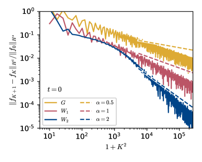
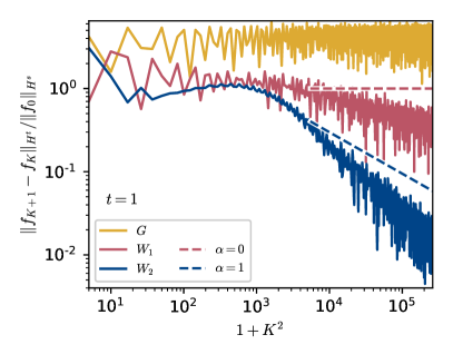
Figure 1: Error estimate $\|f_{K+1}-f_{K}\|_{H^{t}}$ for a circular billiard with constant damping $w(x,y)=\mu=0.9$ as a function of the truncation order $K$ on a double logarithmic scale. Left: $t_{1}=t_{2}=0$ (convergence in $L^{2}$ norm), right: $t_{1}=t_{2}=1$ (point-wise convergence, in essence). Results are displayed for three different initial boundary densities $G$: $s_{2}=1/2$ (yellow, top), $W_{1}$: $s_{2}=1$ (red, middle), $W_{2}$: $s_{2}=2$ (dark blue, bottom), see text. Lines show the power law decay according to equation (21), $\alpha=s_{2}-t_{1}$.

The data shown in Figure 1 confirm the upper bound in Theorem 3.4. For the $L^{2}$ norm, $t_{1}=t_{2}=0$, we observe, in each case, convergence at a rate which is slightly faster than the theoretical prediction $\alpha=s_{2}-t_{1}$. The power law decay of the truncation error shows up for large values of $K$ and the onset of this scaling region shifts towards larger values if the initial boundary density becomes smooth. This should not come as a surprise, since the resolution of higher order derivatives requires higher order Fourier modes. For the parameter at the boundary of point-wise convergence $t=(1,1)$, we see that the discontinuous boundary density fails to converge in line with our theoretical predictions. While Theorem 3.4 does not guarantee convergence in case $W_{1}$ either, the numerical data suggest an extremely slow convergence which is still consistent with the upper bound estimate $\alpha=s_{2}-t_{1}=1-1=0$. Finally, for the smooth boundary density (case $W_{2}$) we observe a convergence rate slightly faster than the theoretical prediction.

From a dynamical perspective, circular billiards are trivial since the billiard map (2) is an integrable twist map. In order to get an idea of how dynamical properties impact on convergence properties we show numerical results for a deformed circle billiard which displays mixed regular and chaotic dynamics. For the deformation we choose the radius to depend on the polar angle $x$ according to

$$r(x)=1+\delta\cos(mx),$$ (22)

where we choose $m=3$ in the following. Deformations of this kind are known in the literature as Limaçon billiards [1]. We will cover the cases $\delta=0.01$ and $\delta=0.1$. For larger values, the billiard fails to be convex. In order to demonstrate the change in dynamical behaviour, Figure 2 shows the Poincare plot of the collision map $T$. For a small value of the deformation, $\delta=0.01$, one still observes a fairly large number of invariant tori in accordance with general KAM folklore. The larger perturbation shown in Figure 2, $\delta=0.1$, destroys most of the regular motion and renders the system chaotic with a few exceptions, for example, the highlighted period-$3$ island.

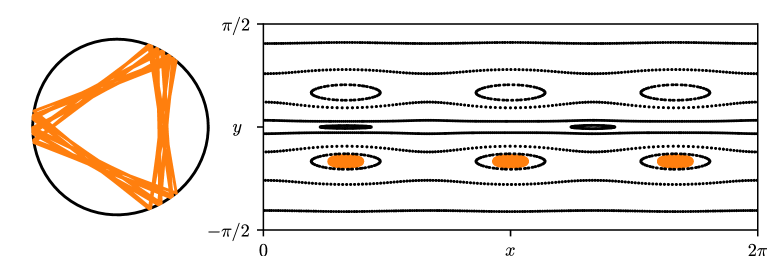
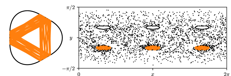
Figure 2: Billiard with orbit in configuration space (left) and Poincare plot of the boundary map $T$ in the $(x,y)$ phase space (right) for a deformed billiard according to (22). Top: weak deformation of the circle ($m=3,\delta=0.01$), bottom: strong but still convex deformation ($m=3,\delta=0.1$). The orbit depicted in real space is highlighted in phase space as well.

In order to calculate the convergence of the energy distribution we have to evaluate the matrix elements of the transfer operator. For the circular billiard, the only non-zero entries take the value $\pm\mu$ and follow the structure given by equation (24). Once the circle has been deformed, the analytic calculation of the matrix elements is no longer possible. Even worse, the collision map is not given in closed analytic form either, so that an efficient numerical calculation becomes a nontrivial task (see the appendix for details). However, we are able to reduce the calculation of the matrix elements to double integrals with the kernel being given in closed analytic form, see equation (25). Nevertheless, the numerical evaluation is still time consuming, in particular, since the matrix is no longer sparse. Hence, we can only calculate finite approximations up to $K=30$. In order to reach the scaling regime (see Figure 1 for comparison) we employ a stronger damping of $\mu=0.1$. The results for the error measured in $L^{2}$ norm, that is, for the choice $t_{1}=t_{2}=0$, are shown in Figure 3.

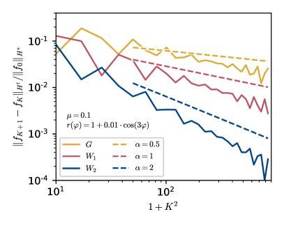
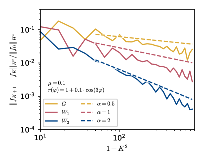
Figure 3: Error estimate $\|f_{K+1}-f_{K}\|_{H^{t}}$ in $L^{2}$ norm, $t=(0,0)$, for the energy density of a Limaçon billiard as a function of the truncation order $K$ on a double logarithmic scale. Constant damping $w(x,y)=\mu=0.1$ and two deformations, $\delta=0.01$ (left) and $\delta=0.1$ (right), are considered. Results are displayed for the three different initial boundary densities $G$: $s_{2}=1/2$ (yellow, top), $W_{1}$: $s_{2}=1$ (red, middle), $W_{2}$: $s_{2}=2$ (dark blue, bottom), see Figure 1. Lines indicate a power law decay, $\alpha=s_{2}-t_{1}$, according to the rigorous estimate for circle billiards.

It is quite remarkable that the decay of the error is apparently almost unaffected by the degree of chaoticity. Hence the rigorous error estimate of Theorem 3.4 which covers the case $\delta=0$ seems to have a wider range of applicability. While intuitively such an observation would not be surprising for nearly integrable cases it is quite counter-intuitive that the same error estimate may hold as well in strongly chaotic situations. However, our proof does not cover any of the deformed billiards and there does not seem to be an obvious way how the methodology can be generalised to these complicated cases. Nevertheless, it is reaffirming that our study of a simple dynamical system like the circular billiard has relevance for more complex dynamical behaviour.

Appendix A Matrix elements

Consider a convex billiard with boundary being given by $r(x)$ in polar coordinates where $x$ denotes the polar angle (see, for example, equation (22)). Denote by $(x^{\prime},y^{\prime})=(T_{x}(x,y),T_{y}(x,y))$ the collision map where $x$ and $x^{\prime}$ label subsequent collisions with the boundary. Using a standard representation in terms of Fourier basis functions [24], the matrix elements $M_{l,k}$ of the transfer operator read

$$M_{l,k} = \frac{1}{2\pi^{2}}\int\limits_{0}^{2\pi}\int\limits_{-\pi/2}^{\pi/2}(\mathcal{C}_{\phi}e_{k})(x,y)\,\overline{e_{l}(x,y)}\,\mathrm{d}y\mathrm{d}x$$

$$= \frac{1}{2\pi^{2}}\int\limits_{0}^{2\pi}\!\!\int\limits_{-\pi/2}^{\pi/2}\!\!\mathrm{e}^{\mathrm{i}k_{1}\phi_{x}(x,y)-\mathrm{i}l_{1}x+2\mathrm{i}k_{2}\phi_{y}(x,y)-2\mathrm{i}l_{2}y}\,\mathrm{d}y\mathrm{d}x$$

with $k=(k_{1},k_{2})$ and $l=(l_{1},l_{2})$.

In case of the perfect circle we get a representation which is given by a sparse matrix with only a few non-zero elements, close to the main diagonal, namely

$$(\mathcal{C}_{\phi}e_{l})(x,y)=\sum\limits_{k\in\mathbb{Z}^{2}}M_{l,k}\cdot e_{k}(x,y)$$ (23)

with the matrix elements

$$M_{l,k}=(-1)^{k_{1}}\,\delta_{k_{1},l_{1}}\,\delta_{l_{2},k_{1}+k_{2}}\,\quad\quad\,\,k,l\in\mathbb{Z}^{2}.$$ (24)

This is the extension of equation (12) to all Fourier modes and it was used to calculate the values for Figure 1.

In order to eliminate the implicitly defined collision map we change integration variables from $(x,y)$ to $(x,x^{\prime})$. Using $y_{1}(x,x^{\prime})=y$ and $y_{2}(x,x^{\prime})=y^{\prime}$ for the two scattering angles the matrix elements become

$$M_{l,k}=\frac{1}{2\pi^{2}}\int\limits_{0}^{2\pi}\!\!\int\limits_{0}^{2\pi}\left|\frac{\partial y_{2}(x,x^{\prime})}{\partial x}\right|\mathrm{e}^{\mathrm{i}(k_{1}x-l_{1}x^{\prime})}\mathrm{e}^{2\mathrm{i}(k_{2}y_{1}(x,x^{\prime})-l_{2}y_{2}(x,x^{\prime}))}\mathrm{d}x^{\prime}\mathrm{d}x,$$ (25)

where the additional factor is the Jacobian of the coordinate transformation. In contrast to the collision map $T$, the expressions $y_{1}(x,x^{\prime})$ and $y_{2}(x,x^{\prime})$ can be obtained in closed analytic form so that equation (25) is easier to implement numerically.

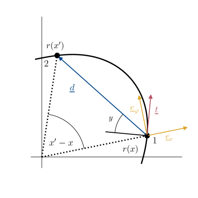
Figure 4: Geometric configuration of two subsequent collisions in a convex billiard with a particle moving from point 1 (with parameter value $x$) to point 2 (with parameter value $x^{\prime}$). We also depict the ray vector $\underline{d}$, the tangent vector $\underline{t}$, and the unit vectors $\underline{e}_{r}$ and $\underline{e}_{\varphi}$ in polar coordinates.

Figure 4 shows a sketch of two subsequent collisions. The first scattering angle $y_{1}$ is given in terms of an inner product

$$\sin(y_{1})=\underline{d}\cdot\underline{t}/(|\underline{d}||\underline{t}|)\,.$$

Since the position vector of the initial point is given by $r(x)\underline{e}_{r}$ the tangent is easily obtained as $\underline{t}=r^{\prime}(x)\underline{e}_{r}+r(x)\underline{e}_{\varphi}$. The vector separating the two points of collision is given in terms of the local basis vectors by

$$\underline{d}=(r(x^{\prime})\cos(x^{\prime}-x)-r(x))\underline{e}_{r}+r(x^{\prime})\sin(x^{\prime}-x)\underline{e}_{\varphi}\,.$$

Hence the closed form expression for the first scattering angle reads

$$\sin(y_{1})=\frac{r^{\prime}(x)(r(x^{\prime})\cos(x^{\prime}-x)-r(x))+r(x)r(x^{\prime})\sin(x^{\prime}-x)}{\sqrt{r^{2}(x)+(r^{\prime}(x))^{2}}\sqrt{r^{2}(x)+r^{2}(x^{\prime})-2r(x)r(x^{\prime})\cos(x^{\prime}-x)}}\,.$$ (26)

The second scattering angle is obtained by interchanging the two points in Figure 4, i.e., by swapping $x$ and $x^{\prime}$ in equation (26), and including an additional minus sign for the outgoing angle

$$\sin(y_{2})=-\frac{r^{\prime}(x^{\prime})(r(x)\cos(x-x^{\prime})-r(x^{\prime}))+r(x^{\prime})r(x)\sin(x-x^{\prime})}{\sqrt{r^{2}(x^{\prime})+(r^{\prime}(x^{\prime}))^{2}}\sqrt{r^{2}(x^{\prime})+r^{2}(x)-2r(x^{\prime})r(x)\cos(x-x^{\prime})}}\,.$$

References

References

[1]
Bäcker A, and Dullin H R,
Symbolic dynamics and periodic orbits
for the cardioid billiard,
J. Phys. A.30 (1997)
1991–2020
[2]
Baladi V, and Holschneider M,
Approximation of nonessential spectrum of transfer operators,
Nonlinearity12 (1999) 525–538
[3]
Baladi V,
Positive Transfer Operators and Decay of Correlations,
World Scientific, Singapore, 2000
[4]
Baladi V,
Dynamical Zeta Functions and Dynamical Determinants for Hyperbolic Maps,
Springer, Cham, 2018
[5]
Boyarsky A, and Gora P,
Laws of Chaos: Invariant Measures and Dynamical Systems in One Dimension,
Birkhäuser, Basel, 1997
[6] Chae K S, Ih J G,
Prediction of vibrational energy distribution in the thin plate at
high-frequency bands by using the ray tracing method,
J. Sound Vib.240 (2001)
263–292
[7] Chappell D J, Löchel D,
Søndergaard N, and Tanner G,
Dynamical energy analysis on mesh grids: A new tool for describing
the vibro-acoustic response of complex mechanical structures,
Wave Motion51 (2014)
589–597
[8] Chappell D J, Tanner G, Löchel D, and
Søndergaard N,
Discrete flow mapping: transport of phase space densities
on triangulated surfaces,
P. Roy. Soc. A469 (2013)
20130153
[9]
Chen J, and Wang H,
Preasymptotics and asymptotics of approximation numbers of anisotropic Sobolev embeddings,
J. Complexity39 (2017)
94–110
[10]
Dellnitz M, Junge O,
On the approximation of complicated dynamical behavior,
SIAM J. Numer. Anal.36 (1999) 491–515
[11]
Dellnitz M, Froyland G, and Sertl S,
On the isolated spectrum of Perron-Frobenius operator,
Nonlinearity 13 (2000) 1171–1188
[12] Deschamps G A,
Ray techniques in electromagnetics,
Proc. IEEE60 (1972)
1022–1035
[13] Haake F,
Quantum Signatures of Chaos,
3rd Ed., Springer, Berlin Heidelberg, 2010
[14]
Hartmann T, Morita S, Tanner G, and Chappell D J,
High-frequency structure- and air-borne sound transmission for
a tractor model using Dynamical Energy Analysis,
Wave Motion87 (2019)
132–150
[15]
Hartmann T, Tanner G, Xie G, Chappell D J, and Bajars J,
Modelling of high-frequency structure-borne sound transmission on
FEM grids using the Discrete Flow Mapping technique,
J. Phys. Conf. Ser.744 (2016)
01237
[16]
Keller G, and Liverani, C,
Stability of the spectrum for transfer operators,
Ann. Scuola Norm. Sup. Pisa Cl. Sci.28 (1999)
141–152
[17]
Klus, S, Koltai P, and Schütte, C,
On the numerical approximation of the Perron-Frobenius and Koopman operator,
J. Comp. Dyn.3 (2016)
57–79
[18]
Kühn T, Sickel W and Ullrich T,
Approximation numbers of Sobolev embeddings—Sharp constants and
tractability,
J. Complexity30(2) (2014)
95–116
[19]
Liverani, C,
Rigorous numerical investigation of the statistical properties of
piecewise expanding maps — A feasibility study,
Nonlinearity14 (2001) 463–490
[20]
Mayer D H,
The Ruelle-Araki Transfer Operator in Classical Statistical Mechanics,
Springer-Verlag, Berlin, 1978
[21]
Ruelle D,
Thermodynamic Formalism: the Mathematical Structures of
Classical Equilibrium Statistical Mechanics,
Addison-Wesley, Reading, 1978
[22] Savioja L and Svensson U P,
Overview of geometrical room acoustic modeling techniques,
J. Acou. Soc. Am.138 (2015) 708–730
[23] Tanner G, and Søndergaard N,
Wave chaos in acoustics and elasticity,
J. Phys. A40 (2007)
R443-R509
[24] Tanner G,
Dynamical energy analysis—Determining wave energy distributions
in vibro-acoustical structures in the high-frequency regime,
J. Sound. Vib.320 (2009)
1023–1038
[25]
Triebel H,
Theory of Function Spaces III,
Birkhäuser, Basel, 1983
[26]
Walker, J S
A Primer on Wavelets and their Scientific Applications,
CRC Press, Boca Raton, 2008