Tight-Binding Studio: A Technical Software Package to Find the Parameters of Tight-Binding Hamiltonian

Abstract

We present Tight-Binding Studio (TBStudio) software package for calculating tight-binding Hamiltonian from a set of Bloch energy bands obtained from first principle theories such as density functional theory, Hartree-Fock calculations or Semi-empirical band structure theory. This will be helpful for scientists who are interested in studying electronic properties of structures using Green’s function theory in tight-binding approximation. TBStudio is a cross-platform application written in C++ with a graphical user interface design that is user-friendly and easy to work with. This software is powered by Linear Algebra Package C interface library for solving the eigenvalue problems and the standard high performance OpenGL graphic library for real time plotting. TBStudio and its examples together with the tutorials are available for download from tight-binding.com

I Introduction

Many researchers are interested in the study of nanostructures and solid state materials in general, but there are many computational and mathematical challenges which hinder rapid progress. Therefore, new computational packages are urgently needed in order to accelerate scientific progress. Here, we are interested in electronic structure properties.

First-principles electronic structure calculations FP are based on the laws of quantum mechanics and only use the fundamental constants of physics as input to provide detailed insight into the origin of mechanical, electronic, optical and magnetic properties of materials and molecules. Both structural and spectroscopic information is directly obtainable from high-performance computations and yields information which is complementary to that obtained from experimental such as transmission electron microscopy data.

Density functional theory (DFT) is one of the most important methods used in electronic structure calculations and computational physics has provided already a diverse number of software packages such as OpenMX openmx , VASP VASP1 ; VASP2 ; VASP3 , QUANTUM ESPRESSO QE and ABINIT ABINIT that are based on different algorithms. The accuracy of different methods depends on the used approximations, e.g. the particular form for the exchange-correlation (XC) energy.

First-principles calculations is commonly applied to calculate the properties of an infinite periodic arrangement of one or more atoms (the basis) repeated at each lattice point that describes a highly ordered structure, occurring due to the intrinsic nature of its constituents to form symmetric patterns. The periodicity can make problems easier, but sometimes it can be a drawback when one is interested in the electronic properties of finite size systems. Linear combination of atomic orbitals (LCAO) lcao1 ; lcao2 is a good candidate to overcome this problem.

The most important justification to setup LCAO is that the combination of this method with Green’s function theory can be also used for non-periodic systems and furthermore, in the case of systems with a huge number of atoms there are a variety of cost and time efficiency motivations which can lead one to use the LCAO method.

Tight-Binding (TB) approaches are based on the LCAO method that is primarily used to calculate the band structure and single-particle Bloch states of a material as e.g. done by Slater and Koster (SK) slaterkoster . The tight-binding method is simple and computationally very fast. Therefore, it is often used in calculations of very large systems, with more than a few thousand atoms in the unit cell. There are a number of earlier reviews  Ackland ; Goringedag that people working in this field should be aware of. TB Hamiltonian gives the electronic structure of a system using a real-space picture of the system. The real Hamiltonians provide insight into the nature of the transport mechanisms.

To find a TB Hamiltonian one needs to evaluate the band-structure of a typical structure based on first principles calculations and construct a tight-binding model via the Slater and Koster method to reproduce the band energies obtained from DFT.

The purpose of this paper is to introduce Tight-Binding Studio (TBStudio), a new technical software package for generating TB Hamiltonians based on Slater-Koster method from data obtained from first principles calculations that has been made available at tight-binding.com. Cross-platform graphical user interface of TBStudio is written in C++ using native controls and emulates foreign functionality via wxWidgets wxWid tools library for GTK, MS Windows, and MacOS. Also, BLAS BLAS and LAPACK LAPACK routines are used for matrix multiplications, solving systems of simultaneous linear equations and eigenvalue problems. The standard high performance OpenGL graphic library openglsite has been used for real time plotting. The main structure of TBStudio and several important topics, including the post processing tools are explained in the rest of this paper.

II Linear Combination of Atomic Orbitals

Consider two atoms which have atomic orbitals described by wave function $\Psi_{A}$ and $\Psi_{B}$. If the atoms are at the equilibrium distance, their electron clouds overlap with each other and the wave function of molecular orbital can be obtained from a linear combination of atomic orbitals as follows

$$\Psi_{AB}=c_{A}\Psi_{A}+c_{B}\Psi_{B}\,,$$ (1)

where $\Psi_{AB}$ is the normalized wave function of molecular orbitals of the molecule AB. With this in mind we are able to expand the Bloch functions as linear combinations of the orbitals $\varphi$ as follows

$$\centering\psi_{k}(\textbf{r})=\sum\limits_{i}\sum\limits_{\nu_{i}}c_{i\nu_{i}}(k)\phi_{\nu_{i},k}(\textbf{r}-\textbf{r}_{i})\,,\@add@centering$$ (2)

where $i$ runs over all unit cell atoms and $\nu_{i}$ runs over the orbitals defined for $i^{th}$ atom and

$$\centering\phi_{\nu,\textbf{k}}(\textbf{r})=\sum\limits_{n\in\mathbb{Z}}\sum\limits_{m\in\mathbb{Z}}\sum\limits_{l\in\mathbb{Z}}e^{i\textbf{k}.\textbf{R}_{n,m,l}}\varphi_{\nu}(\textbf{r}-\textbf{R}_{n,m,l})\,,\@add@centering$$ (3)

in which $\textbf{R}_{n,m,l}$ is the discrete translation vector of the unit cell at $(n,m,l)$ of the Bravais lattice. The electron hopping between different orbitals is an essential ingredient in TB approach. In a simple non-interacting picture, the overlap of the outermost electrons leads to the hybridization of the electronic orbitals and leads to the de-localization of Bloch states.

To calculate the energy bands we should solve the generalized eigenvalue problem

$$\centering\hat{H}(\textbf{k})\psi_{n}^{\sigma}(\textbf{k})=\varepsilon_{n\boldsymbol{k}\sigma}\hat{S}(\textbf{k})\psi_{n}^{\sigma}(\textbf{k})\,,\@add@centering$$ (4)

where $\hat{H}$ and $\hat{S}$ are the TB Hamiltonian and the overlap operators that can be written as

$$\centering\hat{H}\@add@centering =\sum\limits_{i,i^{\prime}}\sum\limits_{\nu_{i},\nu_{i}^{\prime}}\hat{H}|\phi_{\nu_{i}}><\phi_{{\nu^{\prime}}_{i^{\prime}}}|\,,$$

$$\hat{S} =\sum\limits_{i,i^{\prime}}\sum\limits_{\nu_{i},\nu_{i}^{\prime}}|\phi_{\nu_{i}}><\phi_{{\nu^{\prime}}_{i^{\prime}}}|\,,$$ (5)

where in general the basis can be non-orthogonal and then the overlap matrix can be a non-identity matrix. The elements of the Hamiltonian and the overlap matrices can be found by definition of the molecular two-center integrals in terms of the quantities called Slater and Koster integrals.

III Calculation of Slater-Koster integral Table

The most important issue that is the background of the idea of Slater and Koster approach is the rotation operator defined as follows

$${\displaystyle D(\mathbf{\hat{n}},\phi)=\exp\left(-i\phi{\frac{\mathbf{\hat{n}}\cdot\mathbf{J}}{\hbar}}\right)}\,,$$ (6)

and the SK parameters

$$h_{ll^{\prime}}^{mm^{\prime}}(\mathbf{r}) =\left\langle\varphi_{l}^{m}(\mathbf{x}+\mathbf{r})|H(\mathbf{x}+\mathbf{r})|\varphi_{l^{\prime}}^{m^{\prime}}(\mathbf{x})\right\rangle\,,$$

$$s_{ll^{\prime}}^{mm^{\prime}}(\mathbf{r}) =\left\langle\varphi_{l}^{m}(\mathbf{x}+\mathbf{r})|\varphi_{l^{\prime}}^{m^{\prime}}(\mathbf{x})\right\rangle\,,$$ (7)

in which $\varphi_{l}^{m}(\mathbf{x})$ stands for a specific atomic orbital defined by angular quantum numbers $l$ and $m$. Note, the orbitals in Eq. (7) are the real spherical harmonics. Without any change in the basic framework one can rotate the basis vectors as follows

$$h_{ll^{\prime}}^{mm^{\prime}}(\mathbf{r}) =\left\langle\varphi_{l}^{m}(\mathbf{x}+\mathbf{r})|\bar{D}^{\dagger}H(\mathbf{x}+\mathbf{r})\bar{D}|\varphi_{l^{\prime}}^{m^{\prime}}(\mathbf{x})\right\rangle\,,$$

$$s_{ll^{\prime}}^{mm^{\prime}}(\mathbf{r}) =\left\langle\varphi_{l}^{m}(\mathbf{x}+\mathbf{r})|\bar{D}^{\dagger}\bar{D}|\varphi_{l^{\prime}}^{m^{\prime}}(\mathbf{x})\right\rangle\,,$$ (8)

where $\bar{D}=\bar{D}(l,m,n)$ operator is a function of directional cosines defined by the angles of the bond vector between the atoms and the Cartesian basis vectors $\hat{x}$, $\hat{y}$ and $\hat{z}$. The rotation operator for different orbitals can be calculated from the Clebsch-Gordan coefficients. The bar symbol means symmetrized coefficients which are essential to rotate a real spherical harmonic. The complex spherical harmonics will be converted to real spherical harmonics by applying the following operators ($R_{l}$) for the different orbitals

$$R_{0} =\left(\begin{array}[]{c}1\\ \end{array}\right)\,,$$ (10)

$$R_{1} =\left(\begin{array}[]{ccc}\frac{i}{\sqrt{2}}&0&\frac{i}{\sqrt{2}}\\ 0&1&0\\ \frac{1}{\sqrt{2}}&0&-\frac{1}{\sqrt{2}}\\ \end{array}\right)\,,$$ (14)

$$R_{2} =\left(\begin{array}[]{ccccc}\frac{i}{\sqrt{2}}&0&0&0&-\frac{i}{\sqrt{2}}\\ 0&\frac{i}{\sqrt{2}}&0&\frac{i}{\sqrt{2}}&0\\ 0&0&1&0&0\\ 0&\frac{1}{\sqrt{2}}&0&-\frac{1}{\sqrt{2}}&0\\ \frac{1}{\sqrt{2}}&0&0&0&\frac{1}{\sqrt{2}}\\ \end{array}\right)\,.$$ (20)

The integrals of the rotated vectors in the right hand side of Eq. (8) are called SK parameters as ${ss\sigma}$, ${sp\sigma}$, ${pp\sigma}$, ${pp\pi}$, ${sd\sigma}$, ${pd\sigma}$, ${pd\pi}$, ${dd\sigma}$, ${dd\pi}$ and ${dd\delta}$ slaterkoster ; lendi where the first and the second letters are the orbital label as $s$, $p$ and $d$ and the third letter stands for the type of covalent binding which are formed by the overlap of atomic orbitals. ${\sigma}$, ${\pi}$ and ${\delta}$ bonds are related to the relative directions of two typical orbitals.

IV Atomic Spin-Orbit Coupling

Structures including heavy atoms show a considerable spin-orbit effect in their electronic properties socdelta . Experimentally, this phenomenon is detectable as a splitting of spectral lines. The addition of spin-orbit coupling (SOC) to study such materials is known as fine structure. There are many structures soc1 ; soc2 ; soc3 ; soc4 ; soc5 in which taking SOC into accounts becomes very important in atomistic modeling. This effect is a phenomenon that comes from a relativistic interaction of a particle’s spin with its motion inside a potential $\mathbf{V}$ and so the energy level split produced by the SOC is usually of the same order in size to the relativistic corrections to the kinetic energy. SOC fine structure can be added as a term to the Hamiltonian. The atomic spin-orbit interaction may be included in the TB model as

$$\hat{H}_{SO}=\frac{1}{2(m_{e}c)^{2}}(\mathbf{\nabla}\mathbf{V}\times\mathbf{P}).\mathbf{S}\,,$$ (21)

where $\mathbf{P}$ and $\mathbf{S}$ are momentum and spin, respectively. Spin-orbit interactions can be accurately approximated by a local atomic contribution of the form

$$\hat{H}_{SO}=\sum_{i}\sum_{\nu}\hat{P}_{i,\nu}\lambda_{\nu}\mathbf{L}_{i}.\mathbf{S}_{i}\,,$$ (22)

in which $\hat{P}_{i,\nu}$ is the projection operator for angular momentum $\nu$ on site $i$ and $\lambda_{\nu}$ denotes the SOC constant for the angular momentum $\nu$, and $S_{i}$ is the spin operator on site $i$. The additional term in the Hamiltonian can be found by calculating the $\mathbf{L}\otimes\mathbf{S}$ operator. The angular and spin operators can be written as follows

$$\mathbf{L}=(L_{x},L_{y},L_{z})\,,$$

$$\mathbf{S}=(S_{x},S_{y},S_{z})\,,$$ (23)

where

$$L_{x}=\frac{L^{+}+L^{-}}{2}\,,$$

$$L_{y}=\frac{L^{+}-L^{-}}{2i}\,,$$ (24)

in which $L^{+,-}$ denote the ladder operators for the orbitals. Similarly, we obtain $S_{x}$ and $S_{y}$ in terms of the $S^{+,-}$ ladder spin operators. Note that we need the operator to be compatible with the real spherical harmonics. The real SOC operator can be evaluated as follows

$$\bar{R}_{l}.(\mathbf{L}\otimes\mathbf{S}).\bar{R}_{l}^{-1}\,,$$ (25)

where

$$\bar{R}_{l}=R_{l}\otimes I_{2\times 2}\,.$$ (26)

One should find the final results for the different $s$, $p$ and $d$ orbitals as listed in Table 1.

Table 1: The real spherical harmonics for different angular quantum numbers $l$ and $m$.

l	$0$	$1$	$1$	$1$	$2$	$2$	$2$	$2$	$2$
m	$0$	$-1$	$0$	$1$	$-2$	$-1$	$0$	$1$	$2$
Real spherical harmonic	$\quad s\quad$	$\quad p_{y}\quad$	$\quad p_{z}\quad$	$\quad p_{x}\quad$	$\quad d_{\text{xy}}\quad$	$\quad d_{\text{yz}}\quad$	$\quad d_{3z^{2}-r^{2}}\quad$	$\quad d_{\text{xz}}\quad$	$\quad d_{x^{2}-y^{2}}\quad$

$$\centering\hat{H}_{s}^{SOC}=\lambda_{s}\mathbf{L_{s}}\otimes\mathbf{S}=\left(\begin{array}[]{cc}0&0\\ 0&0\\ \end{array}\right)\,,\@add@centering$$

$$\centering\hat{H}_{p}^{SOC}=\lambda_{p}\mathbf{L_{p}}\otimes\mathbf{S}=\lambda_{p}\quad\blockarray{*{6}{c}l}\block{*{6}{>{\footnotesize}c<{}}l}p_{y}&p_{y}p_{z}p_{z}p_{x}p_{x}\\ \block{(*{6}{c})>{\footnotesize}l<{}}0&00\frac{i}{2}-\frac{i}{2}0\quad p_{y}\\ 00\frac{i}{2}00\frac{i}{2}\quad p_{y}\\ 0-\frac{i}{2}000\frac{1}{2}\quad p_{z}\\ -\frac{i}{2}000-\frac{1}{2}0\quad p_{z}\\ \frac{i}{2}00-\frac{1}{2}00\quad p_{x}\\ 0-\frac{i}{2}\frac{1}{2}000\quad p_{x}\\ \,\,\,,\@add@centering$$

$$\centering\hat{H}_{d}^{SOC}=\lambda_{d}\mathbf{L_{d}}\otimes\mathbf{S}=\lambda_{d}\quad\blockarray{*{10}{c}l}\block{*{10}{>{\footnotesize}c<{}}l}d_{\text{xy}}&d_{\text{xy}}d_{\text{yz}}d_{\text{yz}}d_{3z^{2}-r^{2}}d_{3z^{2}-r^{2}}d_{\text{xz}}d_{\text{xz}}d_{x^{2}-y^{2}}d_{x^{2}-y^{2}}\\ \block{(*{10}{c})>{\footnotesize}l<{}}0&00-\frac{1}{2}000\frac{i}{2}-i0\quad d_{\text{xy}}\\ 00\frac{1}{2}000\frac{i}{2}00i\quad d_{\text{xy}}\\ 0\frac{1}{2}000\frac{i\sqrt{3}}{2}-\frac{i}{2}00\frac{i}{2}\quad d_{\text{yz}}\\ -\frac{1}{2}000\frac{i\sqrt{3}}{2}00\frac{i}{2}\frac{i}{2}0\quad d_{\text{yz}}\\ 000-\frac{i\sqrt{3}}{2}000\frac{\sqrt{3}}{2}00\quad d_{3z^{2}-r^{2}}\\ 00-\frac{i\sqrt{3}}{2}000-\frac{\sqrt{3}}{2}000\quad d_{3z^{2}-r^{2}}\\ 0-\frac{i}{2}\frac{i}{2}00-\frac{\sqrt{3}}{2}000\frac{1}{2}\quad d_{\text{xz}}\\ -\frac{i}{2}00-\frac{i}{2}\frac{\sqrt{3}}{2}000-\frac{1}{2}0\quad d_{\text{xz}}\\ i00-\frac{i}{2}000-\frac{1}{2}00\quad d_{x^{2}-y^{2}}\\ 0-i-\frac{i}{2}000\frac{1}{2}000\quad d_{x^{2}-y^{2}}\\ \,\,\,.\@add@centering$$

Please note that when we use the operators (20), the order of the matrix elements are not the same as complex spherical harmonics and depends on the definition of the transformation matrix ($R_{l}$). In this work, the order of the real spherical harmonics are presented in Table 1.

V Iterative Minimization

TBStudio algorithm is based on the Levenberg–Marquardt least-squares curve fitting approach in which we have a set of data obtained from first-principles calculation and an analytical expression representing the TB model for which we have to find the best independent parameters. Generally, the sum of the squares of the deviations may be written as follows

$$S(\boldsymbol{\beta})=\sum\limits_{n}\sum\limits_{\boldsymbol{k}}\sum\limits_{\sigma}(\varepsilon_{n\boldsymbol{k}\sigma}^{\prime}-\varepsilon_{n\boldsymbol{k}\sigma}(\boldsymbol{\beta}))^{2}\,,$$

where $\varepsilon$ and $\varepsilon^{\prime}$ are, respectively, the TB results and DFT band energies and $\boldsymbol{\beta}$ is a parameter vector that is a set of independent variables i.e. SK parameters and overlap integrals and SOC. Non-linear least square minimization problems arise especially in curve fitting where here the curves are energy bands which are highly coupled to each other. To start the minimization, the user has to provide an initial guess for $\boldsymbol{\beta}$ and using the guessed $\boldsymbol{\beta}$ and the mentioned SK parameters one can find the TB band energies and also the Jacobian matrix

$$J_{n\boldsymbol{k}\sigma,j}=\frac{\partial\varepsilon_{n\boldsymbol{k}\sigma}(\boldsymbol{\beta})}{\partial\boldsymbol{\beta}_{j}}\,.$$

In each iteration, we replace $\boldsymbol{\beta}$ by a new parameter vector $\boldsymbol{\beta}+\boldsymbol{\delta}$ in which $\boldsymbol{\delta}$ is a correction vector that can be estimated by first order Taylor series expansion of TB band energies as follows

$$\varepsilon_{n\boldsymbol{k}\sigma}(\boldsymbol{\beta}+\boldsymbol{\delta})=\varepsilon_{n\boldsymbol{k}\sigma}(\boldsymbol{\beta})+{\boldsymbol{J}}_{n\boldsymbol{k}\sigma}.{\boldsymbol{\delta}}\,.$$

At optimum values for the independent variables, the sum of square deviations has reached its minimum with respect to the independent vector and we have

$$\frac{\partial S(\boldsymbol{\beta}+\boldsymbol{\delta})}{\partial\boldsymbol{\delta}}=0\,,$$ (27)

which however may also result in local minima. Depending on the problem and the system and the number of degrees of freedom, there might be many local minima which occur when the objective function value is greater than its value at the so-called global minimum. When multiple minima exist the important consequence is that the objective function definitely has a maximum value somewhere between two minima which makes it difficult to obtain a good fitting. Refinement from a bad SK parameter point (a set of independent parameter values $\boldsymbol{\beta}_{0}$) close to a physically unknown local minimum will be ill-conditioned and should be avoided as a starting point. Because generally we do not have an analytical expression for the TB band structure, we can not analyze the location of local minima in detail. Band structure curves have complex forms for which it is either very difficult or even impossible to derive analytical expressions for the elements of the Jacobian. In such cases, we need to find the elements by using numerical approximations as follows

$$\frac{\partial\varepsilon_{n\boldsymbol{k}\sigma}(\boldsymbol{\beta})}{\partial\boldsymbol{\beta}_{j}}\approx\frac{\varepsilon_{n\boldsymbol{k}\sigma}(\boldsymbol{\beta}+\boldsymbol{\delta})-\varepsilon_{n\boldsymbol{k}\sigma}(\boldsymbol{\beta}-\boldsymbol{\delta})}{2\boldsymbol{\delta}_{j}}\,.$$

VI Explicit form for the Tight-Binding Hamiltonian

Fig. 1 shows a schematic representation of the TB model. The mono-electronic Hamiltonian $H$ and the overlap matrix $S$ may be rewritten as

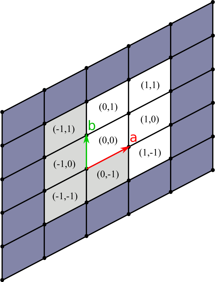
Figure 1: Schematic representation of the TB model for a typical 2D crystal. The red (a) and green (b) vectors are the unit vectors and the white cells indicate independent unit cells.

$$\centering\hat{H}=\sum\limits_{n\in\mathbb{Z}}\sum\limits_{m\in\mathbb{Z}}\sum\limits_{l\in\mathbb{Z}}\hat{h}_{l,n,m}e^{i\mathbf{k}.\mathbf{R}_{l,m,n}}\,,\@add@centering$$ (28)

and

$$\centering\hat{H}=\sum\limits_{n\in\mathbb{Z}}\sum\limits_{m\in\mathbb{Z}}\sum\limits_{l\in\mathbb{Z}}\hat{s}_{l,n,m}e^{i\mathbf{k}.\mathbf{R}_{l,m,n}}\,.\@add@centering$$ (29)

Since H and S are Hermitian, therefore

$$\centering\hat{h}_{-n,-m,-l}\@add@centering =\hat{h}_{n,m,l}^{\dagger}\,,$$

$$\hat{s}_{-n,-m,-l} =\hat{s}_{n,m,l}^{\dagger}\,,$$ (30)

and thus, in this two dimensional example, we have only five independent matrices. As shown in Fig. 1 we must determine only the matrices h and s for the cells at $(0,0)$, $(1,0)$, $(0,1)$, $(1,1)$ and $(-1,1)$. Using the SK coefficients we can calculate the Hamiltonian and the overlap matrix and extract the matrices h and s. TBStudio generates the Hamiltonian and overlap matrix for any independent unit cell. Also the code generator tool builds Eqs. (28) and (31) in other desired programming languages. Also, one can use the outputs from TBStudio for post-processing in other transport packages. There are many useful packages for fast calculation of various physical properties of tight-binding models such as PyBinding cPyBinding , Kite cKite , Kwant cKwant , GPUQT GPUQT , TBTK TBTK , PythTB PythTB and WannierTools WannierTools .

After determining the Hamiltonian and the overlap matrix, one can easily calculate the eigenstates and the Bloch functions as well using Eqs. (2) and (3). The $i^{th}$ Wannier function (WF) for the cell $(l,m,n)$ is the Fourier coefficient of $\psi_{i,k}(\textbf{r})$ as follows

$$\centering\textit{w}_{i}^{l,m,n}(r)=\frac{V}{8\pi^{3}}\int{\boldsymbol{d}}^{3}\boldsymbol{k}e^{-i\boldsymbol{k}.\boldsymbol{R}_{l,m,n}}\psi_{i,k}(\textbf{r})\,.\@add@centering$$ (31)

The WF calculated by this method is very close to the real chemical bonding and provides a reliable insight into the nature of the orbitals in the study of electronic properties of solids. It should be noted that, in this way we do not have the problem which we encounter in finding WFs using Maximally Localized Wannier Functions (MLWF) method MLWF . Practically, MLWF algorithms change the shape of WF mathematically to find a perfect fitting to regenerate the band-structure obtained by first-principle methods, because a set of WFs which can generate the obtained band-structure is not unique and may physically not a good set of atomic-orbital-like WFs. In such algorithms that has been implemented in Wannier90 wannier90 and OpenMX openmx , to achieve a physically reliable set of WFs one needs to have a good initial guess and also follow the symmetry adapted methods, but it results in computational difficulties and convergence failure.

VII Summary

In summary, Tight-Binding Studio (TBStudio) is a user-friendly application in the field of quantum computing simulation. The significant parts and important abilities of the TBStudio were briefly mentioned. In short, using this software one can calculate the electron hopping between different orbitals of different atoms and generate an explicit Hamiltonian matrix to do post calculations using Green’s function theory. TBStudio are the density functional theory and the Green’s function theory in the tight-binding approximation. TBStudio is the first step of simulating electronic properties of solids and nanostructures (ie. dispersion, transmission, density of states, current, etc). Also, it is able to calculate thermodynamic properties by means of statistical mechanics approaches.

VIII Data Availability

The supporting information and several examples are available at tight-binding.com. The examples and the supporting codes in additional programming languages, i.e. Matlab, Mathematica, Python, C, C++ and Fortran are also accessible through Code Generator tools in TBStudio.

Acknowledgements This work was supported by the Methusalem program of the Flemish government and M. Nakhaee was supported by a BOF-fellowship (UAntwerpen).

References

- (1) A. R. Leach, Molecular modelling: principles and applications, (Harlow, Prentice Hall, 2001).
- (2) S. Boker, M. Neale, H. Maes, M. Wilde, M. Spiegel, T. Brick, J. Spies, R. Estabrook, S. Kenny, T. Bates, P. Mehta and J. Fox, Psychometrika 76, 306 (2011).
- (3) G. Kresse and J. Hafner Phys. Rev. B 47, 558 (1993).
- (4) G. Kresse and J. Furthmuller, Comput. Mater. Sci. 6, 15 (1993).
- (5) G. Kresse and J. Furthmuller, Phys. Rev. B 54, 11169 (1993).
- (6) S. Scandolo, P. Giannozzi, C. Cavazzoni, S. de Gironcoli, A. Pasquarello, and S. Baroni, Z. Kristallogr. Cryst. Mater. 220, 574 (2005).
- (7) X. Gonze, J.M. Beuken, R. Caracas, F. Detraux, M. Fuchs, G.M. Rignanese, L. Sindic, M. Verstraete, G. Zerah, F. Jollet, and M. Torrent, Comput. Mat. Sci. 25, 478 (2002).
- (8) T. Clark and R. Koch, Linear Combination of Atomic Orbitals (Springer, Berlin, Heidelberg, 1999).
- (9) G. Grosso, Giuseppe Pastori Parravicini-Solid State Physics, 2rd edn. (Academic Press, 2013).
- (10) J. C. Slater and G. F. Koster, Phys. Rev. 94, 1498 (1954).
- (11) G. J. Ackland, M. W. Finnis and V. Vitek, Journal of Physics F: Metal Physics 18, 153 (1988).
- (12) C M Goringedag, D R Bowlerdag, and E Hernándezddag Rep. Prog. Phys. 60, 12, 1447 (1997).
- (13) J. Smart and S. Csomor, Cross-platform GUI programming with wxWidgets (Prentice Hall Professional, 2005).
- (14) C. L. Lawson, R. J. Hanson, D. Kincaid, and F. T. Krogh, ACM Trans. Math. Software 5, 308 (1979).
- (15) E. Anderson, Z. Bai, C. Bischof, S. Blackford, J. Demmel, J. Dongarra, J. Du Croz, A. Greenbaum, S. Hammarling, A. McKenney and D. Sorensen, LAPACK User’s Guide, 3rd edn. (Philadelphia, PA, 1999).
- (16) M. Woo, J. Neider, T. Davis, and D. Shreiner, OpenGL programming guide: the official guide to learning OpenGL (Addison-Wesley Longman Publishing Co., Inc. 1999).
- (17) K. Lendi, Phys. Rev. B 9, 2433 (1974).
- (18) F. Herman, C.D. Kuglin, K.F. Cuff, and R.L. Kortum, Phys. Rev. Lett. 11, 541 (1963).
- (19) H.J. Noh, H. Koh, S.J. Oh, J.H. Park, H.D. Kim, J.D. Rameau, T. Valla, T.E. Kidd, P.D. Johnson, Y. Hu, and Q. Li, EPL (Europhysics Letters) 81, 57006 (2008).
- (20) G. Dresselhaus, Physical Review 100, 580 (1955).
- (21) M. Sakano, M.S. Bahramy, A. Katayama, T. Shimojima, H. Murakawa, Y. Kaneko, W. Malaeb, S. Shin, K. Ono, H. Kumigashira, and R. Arita, Phys. Rev. Lett. 110, 107204 (2013).
- (22) B.A. Bernevig, T.L. Hughes, and S.C. Zhang, Science 314, 1757 (2006).
- (23) A.V. Shevelkov, E.V. Dikarev, R.V. Shpanchenko, and B.A. Popovkin, J. Solid State Chem. 114, 379 (1995).
- (24) D. Moldovan, M. Anđelković, and F. Peeters, PyBinding: A Python package for tight-binding calculations, DOI: 10.5281/zenodo.826942
- (25) S. M. João, M. Anđelković, L. Covaci, T. Rappoport, J.M.V.P. Lopes, and A. Ferreira, DOI: 10.5281/zenodo.3245011
- (26) C. W. Groth, M. Wimmer, A. R. Akhmerov, X. Waintal, Kwant: a software package for quantum transport, New J. Phys. 16, 063065 (2014).
- (27) Z. Fan, V. Vierimaa, and A. Harju, Comput. Phys. Commun. 230, 113 (2018).
- (28) K. Björnson, SoftwareX 9, 205 (2019).
- (29) S. Coh and D. Vanderbilt, Python tight binding (PythTB) code. (2018).
- (30) Q. Wu, S. Zhang, H.F. Song, M. Troyer, and A.A. Soluyanov, Comput. Phys. Commun. 224, 405 (2018).
- (31) I. Souza, N. Marzari, and D. Vanderbilt, Phys. Rev. B 65, 035109 (2001).
- (32) A.A. Mostofi, J.R. Yates, G. Pizzi, Y.S. Lee, I. Souza, D. Vanderbilt, and N. Marzari, Comput. Phys. Commun. 185, 2309 (2014).