Electric double layers with surface charge modulations: Novel exact Poisson-Boltzmann solutions

Abstract

Poisson-Boltzmann theory is the cornerstone for soft matter electrostatics. We provide novel exact analytical solutions to this non-linear mean-field approach, for the diffuse layer of ions in the vicinity of a planar or a cylindrical macroion. While previously known solution are for homogeneously charged objects, the cases worked out exhibit a modulated surface charge –or equivalently surface potential– on the macroion (wall) surface. In addition to asymptotic features at large distances from the wall, attention is paid to the fate of the contact theorem, relating the contact density of ions to the local wall charge density. For salt-free systems (counterions only), we make use of results pertaining to the two-dimensional Liouville equation, supplemented by an inverse approach. When salt is present, we invoke the exact two-soliton solution to the 2D sinh-Gordon equation. This leads to inhomogeneous charge patterns, that are either localized or periodic in space. Without salt, the electrostatic signature of a charge pattern on the macroion fades exponentially with distance for a planar macroion, while it decays as an inverse power-law for a cylindrical macroion. With salt, our study is limited to the planar geometry, and reveals that pattern screening is exponential.

I Introduction

Charges are omnipresent at the microscopic level in soft matter and biological systems Andelman06 . In a solvent like water, featuring efficient solvation and screening properties, surface groups dissociate from large macromolecules (colloids), which results in mobile counterions in the vicinity of charged surfaces. While mobile ions are generically of both signs (both co- and counter-ions), it is possible to approach experimentally the limit of deionized –or salt-free– suspensions Palberg04 , where co-ions are absent. This provides a convenient venue for theoretical investigations, that have studied thermal equilibrium both in the weak-coupling Attard88 ; Podgornik90 ; Netz00 and in the strong-coupling Moreira00 ; Netz01 ; Moreira02a ; Kanduc07 ; Jho08 ; Kanduc08 ; Samaj11 ; Samaj16 ; Samaj18 regimes.

A pillar for the theoretical description of the structure of mobile ions in the vicinity of charged colloids, the so-called electric double-layer, is provided by the Poisson-Boltzmann theory (PB). It dates back to the pioneering works of Gouy Gouy10 and Chapman Chapman13 more than a century ago: it amounts to relating the local charge density appearing in Poisson equation to the Boltzmann weight of the mean electrostatic potential. In doing so, one considers the mobile charged species as an inhomogeneous ideal gas, in a self-consistently determined (although external) electric field, see e.g. the reviews Attard96 ; Hansen00 ; Levin02 ; Messina09 . Electrostatic and steric correlations are thereby neglected, an approach which requires to work in the weak coupling regime. Such a mean-field approximation led to the DLVO theory Verwey48 , that proved essential for rationalizing colloidal interactions.

Analytical solutions of electrostatic theories are useful, allowing to understand the combined effects for the different parameters, such as charge density, temperature, solvent or electrolyte type etc. Screening properties in particular stand foremost, and will receive particular attention below. Previously known explicit analytical exact solutions to the Poisson-Boltzmann theory are scarce unfortunately, essentially limited to

• a single uniformly charged infinite plate with or without salt, two plates or a collection of equi-spaced parallel such plates in the salt-free case Andelman06 ; Attard96 ; Hansen00 ; Levin02 ; Messina09 ; Polat . Such a geometry is relevant for studying lamellar phases Dubois98 .

• a cylindrical colloid, such as DNA, when bending and edge effects are neglected, leading to the infinite cylinder model. Exact results were obtained in the 1950s for a cylindrical concentric Wigner-Seitz cell without salt Alfrey . This solution appears as a restricted version of that for a partial differential equation first studied and solved by Liouville in the 1850s Liouville1853 . More recently, Tracy and Widom obtained a nontrivial exact solution for a single infinite straight and homogeneously charged line Tracy . Exact but perturbative treatments were proposed to account for the finite extension of the charged cylinder TT06 , which in turn led to an accurate description for the persistence length of semi flexible polymers ShenTrizac ; Guilbaud .

To the best of our knowledge, no exact result has been reported for heterogeneously charged macroions. It is our purpose here to put forward a number of such solutions, with or without salt, and to discuss the corresponding screening features. To this end, two techniques will be advocated: the two-dimensional (2D) Liouville artillery for salt-free systems, and the soliton method for solving the 2D sinh-Gordon equation. Since these approaches are two-dimensional in spirit, their translation to a three-dimensional (3D) problem necessarily leads to invariance along one Cartesian coordinate, see below.

A number of experimental “anomalies” –pertaining to particle flocculation, adhesion or deposition– have been attributed to charge heterogeneities or patterns Walz98 . Early theoretical studies of systems with surface charge modulations were based on liquid-state approximations Chan80 ; Kjellander88b ; Gonzalez01 . The combination of Monte-Carlo simulations with analytic perturbation techniques to charged-modulated surfaces in the strong coupling Moreira02b and weak or intermediate coupling Lukatsky02a ; Henle04 regimes indicates, for the studied forms of modulations, an increase of the mean counterion density close to the inhomogeneously charged surfaces, in comparison with that for the uniformly charged surfaces of the same averaged charge density. The notable amplification of this counterion surface enhancement occurs at planar surfaces with disordered surface charge distributions Fleck05 . For two parallel charge-modulated surfaces the enhancement of counterion density near the surfaces means less charges at the midplane, and therefore leads to a reduction of the pressure between the charged plates Lukatsky02b ; Khan05 ; rque10 .

Our interest will be twofold, with focus on both short distance and long-distance features. In the former category, relating the ionic density at contact with the wall, to the surface charge, is of particular interest. For the geometry of one uniformly charged planar wall, the contact theorem provides an exact and particularly simple answer Henderson78 ; Henderson79 ; Carnie81 ; Wennerstrom82 , see the review Blum92 . The generalization of the contact relation to curved wall boundaries was the subject of a number of studies Blum94 ; Trizac97 ; Mallarino15 ; Malgaretti18 . Here, we construct a PB generalization of the contact relation between the density profile at the wall and the inhomogeneous surface charge density, based on the fact that the total force acting on the wall must vanish in thermal equilibrium. All exact solutions fulfill this nonlocal contact relation, but interestingly, some of the solutions provide a local relationship between the total particle number density at the wall surface and the inhomogeneous surface charge density.

Turning to long-distances properties, the decay of density profiles depends on the model under scrutiny. For charged plates, we will show that the influence of a charge pattern on the surface decays exponentially fast away from the plate, irrespective of the presence of salt. This applies in particular to the planar no-salt case, where the density profile goes to zero at large distances from the wall more slowly than an exponential, as an inverse power-law of type $1/x^{2}$ Andelman06 . This asymptotic behavior is universal in the sense that it does not depend on the strength of the surface charge density. For a cylindrical macroion, a charge pattern on the surface of the cylinder extends further than for plates, with a pattern screening of inverse power-law type, the exponent of which will be worked out.

The paper is organized as follows. The general formulation of the models studied, together with their PB treatment are given in Sec. II. The contact relation between the particle density and the surface charge density, known hitherto for uniformly charged plates, is generalized to modulated surface charges. Based on the general solution of the 2D Liouville equation, exactly solvable cases for surface charge modulations with counterions only are generated in an inverse fashion in Sec. III. The explicit results for the potential and particle density are analyzed close, and far away from the charged interface. The results are relevant for both planar and cylindrical geometries. Sec. IV deals with models with added salt. The case of small charges is first worked out (Debye-Hückel perturbative treatment). The exact non-perturbative 2-soliton solution of the nonlinear 2D sinh-Gordon equation is then presented. Sec. V brings a short recapitulation of the most important results.

II General framework

II.1 Relevant boundary conditions

We are interested in the electrostatic potential created by a charged macroion in the 3D Euclidean space of points ${\bf r}=(x,y,z)$. It is sufficient here to restrict our study to the exterior of the macroion, a region that we shall denote as $\Lambda$. The presence of the macroion materializes through the boundary conditions fulfilled by the potential. Classical point-like particles of (say elementary) charge $e$ can move in $\Lambda$. They are immersed in a medium of dielectric constant $\varepsilon$. The wall surface carries a fixed surface charge density $\sigma e$, that can be position dependent. The system is in thermal equilibrium at some inverse temperature $\beta=1/(k_{\rm B}T)$.

The interaction energy of two charges $q$ and $q^{\prime}$ at the points ${\bf r}$ and ${\bf r}^{\prime}$ in $\Lambda$ is given by $qq^{\prime}/(\varepsilon|{\bf r}-{\bf r^{\prime}}|)$. The Bjerrum length

$$\ell_{\rm B}=\frac{\beta e^{2}}{\varepsilon}$$ (2.1)

is the distance between two unit charges at which they interact with thermal energy $k_{\rm B}T$. For a uniform surface charge density $\sigma e$, there exists another relevant length scale. Since the potential energy of a unit charge at distance $z$ from such a wall is $2\pi e^{2}\sigma z/\varepsilon$, this energy equals to $k_{\rm B}T$ at the so-called Gouy-Chapman length

$$\mu=\frac{1}{2\pi\ell_{\rm B}\sigma}.$$ (2.2)

The introduction of $\mu$ is a priori meaningful only for uniform surface charge densities.

Let $\rho({\bf r})$ be the mean charge density of particles at point ${\bf r}\in\Lambda$. Denoting by $\psi({\bf r})$ the corresponding mean electrostatic potential, the electric field is given by

$${\bf E}=-\nabla\psi.$$ (2.3)

The electric field can be decomposed into its perpendicular and parallel components with respect to the wall surface (that may be curved, see below the cylindrical geometry): ${\bf E}=(E_{\perp},{\bf E}_{\parallel})$ where

$$E_{\perp}=-\frac{\partial\psi}{\partial x},\qquad{\bf E}_{\parallel}=-\left(\frac{\partial\psi}{\partial y},\frac{\partial\psi}{\partial z}\right).$$ (2.4)

Gauss’s law demands that Jackson98

$$\nabla\cdot{\bf E}=\frac{4\pi}{\varepsilon}\rho$$ (2.5)

and the mean potential therefore fulfills the Poisson equation

$$\Delta\psi=-\frac{4\pi}{\varepsilon}\rho.$$ (2.6)

The surface charge density $\sigma e$ is related to the normal derivative of $\psi$ at the wall as follows Jackson98

$$\frac{\partial\psi(x,y,z)}{\partial x}\Big{|}_{x=0}=-\frac{4\pi\sigma(y,z)e}{\varepsilon}.$$ (2.7)

The overall system charge neutrality requires that the electric field vanishes at infinite distance from the wall:

$$\lim_{x\to\infty}\frac{\partial\psi}{\partial x}\to 0,$$ (2.8)

where $x$ is a proxy for the distance to the charged macroion. We thus consider here the infinite dilution limit, with a single, field creating, charged body.

II.2 Poisson-Boltzmann theory

We will address two distinct situations:

• For counterions only systems, all mobile particles have the same charge, say $-e$. Denoting by $n({\bf r})$ the particle number density at point ${\bf r}\in\Lambda$, the charge density is simply given by $\rho({\bf r})=-en({\bf r})$. Due to the requirement of overall electroneutrality, the particle density must vanish at asymptotically large distances from the wall, i.e.

  $$\lim_{x\to\infty}n({\bf r})\to 0.$$ (2.9)

  In the standard mean-field approach, the particle density at a given point is proportional to the Boltzmann weight of the mean electrostatic potential at that point Andelman06 ,

  $$n({\bf r})=f_{0}\exp\left[\beta e\psi({\bf r})\right],$$ (2.10)

  where $f_{0}$ is a normalization constant. Introducing the reduced potential $\phi=\beta e\psi$, this mean-field assumption applied to (2.6) leads to the Poisson-Boltzmann (PB) equation

  $$\Delta\phi=4\pi\ell_{\rm B}f_{0}e^{\phi},\qquad n=f_{0}e^{\phi}.$$ (2.11)

  Note a gauge freedom in shifting $\phi$ by a constant which only renormalizes $f_{0}$. The boundary conditions (2.7) and (2.8) read

  $$\frac{\partial\phi}{\partial x}\Big{|}_{x=0}=-4\pi\ell_{\rm B}\sigma,\qquad\lim_{x\to\infty}\frac{\partial\phi}{\partial x}\to 0.$$ (2.12)

  The asymptotic vanishing of the particle density (2.9) means that $\phi$ goes to $-\infty$ as $x\to\infty$.

• For systems with salt, namely the symmetric two-component plasma, we consider two kinds of mobile particles with charges $+e$ and $-e$. Denoting the number densities of positively and negatively charged species by $n_{+}({\bf r})$ and $n_{-}({\bf r})$, the total particle number density is given by

  $$n({\bf r})=n_{+}({\bf r})+n_{-}({\bf r})$$ (2.13)

  and the charge density reads as

  $$\rho({\bf r})=e\left[n_{+}({\bf r})-n_{-}({\bf r})\right].$$ (2.14)

  The system is electroneutral in the bulk region $(x\to\infty)$, so that the bulk species densities must satisfy $n_{+}=n_{-}=n/2$, $n$ being the (prescribed) total bulk density of particles. Within the mean-field assumption for position-dependent species densities

  $$n_{\pm}({\bf r})=n_{\pm}\exp[\mp\beta e\psi({\bf r})],$$ (2.15)

  $\psi({\bf r})$ must go to $0$ as $x\to\infty$. Defining the inverse Debye length $\kappa=\sqrt{4\pi\ell_{\rm B}n}$ and with regard to the Poisson Eq. (2.6), the PB equation for the reduced potential $\phi=\beta e\psi$ reads as

  $$\Delta\phi({\bf r})=\kappa^{2}\sinh\phi({\bf r}),$$ (2.16)

  and we have

  $$\phantom{aaa}n({\bf r})=n\cosh\phi({\bf r}),\quad\rho({\bf r})=-en\sinh\phi({\bf r}).$$ (2.17)

  The boundary condition (2.12) for the reduced potential at the wall ($x=0$) remains unchanged, while the boundary conditions at a symptotically large distances from the wall take the forms

  $$\lim_{x\to\infty}\phi\to 0,\qquad\lim_{x\to\infty}\frac{\partial\phi}{\partial x}\to 0.$$ (2.18)

II.3 Generalization of the contact relation for a planar interface

We aim at generalizing to the inhomogeneous case the contact relation between the particle and uniform surface charge densities. We restrict here to a planar wall, located at $x=0$. We start with the definition of the pressure tensor in a charged medium Landau84

$$\tensor{\bm{\Pi}}({\bf r})=\left[k_{\rm B}Tn({\bf r})+\frac{\varepsilon}{8\pi}{\bf E}^{2}({\bf r})\right]\tensor{\bm{I}}-\frac{\varepsilon}{4\pi}{\bf E}({\bf r})\otimes{\bf E}({\bf r}),$$ (2.19)

where $\tensor{\bm{I}}$ is the unity tensor. The pressure tensor satisfies the mechanical equilibrium condition

$$\bm{\nabla}\cdot\tensor{\bm{\Pi}}={\bf 0}.$$ (2.20)

A surface element $d{\bf S}$ of the wall at $x=0$, which is a vector perpendicular to the surface, is subject to the force

$$d{\bf F}=\tensor{\bm{\Pi}}\cdot d{\bf S}=\left[k_{\rm B}Tn+\frac{\varepsilon}{8\pi}\left(E_{\perp}^{2}+{\bf E}_{\parallel}^{2}\right)-\frac{\varepsilon}{4\pi}E_{\perp}^{2}\right]d{\bf S},$$ (2.21)

where all quantities are dependent on the $(y,z)$-coordinates of the surface element. Now let us place a parallel planar wall with no surface charge at $x\to\infty$. Since for neutral systems, ${\bf E}$ vanishes at $x\to\infty$, we have the force $d{\bf F}^{\prime}=k_{\rm B}Tn_{\rm bulk}d{\bf S}^{\prime}$ where the surface element on the oppositely oriented wall at $x\to\infty$ $d{\bf S}^{\prime}=-d{\bf S}$ and $n_{\rm bulk}$ is the uniform bulk particle density. The total (osmotic) pressure at point $(y,z)$ is thus given by

$$P(y,z) = k_{\rm B}T\left[n(0,y,z)-n_{\rm bulk}\right]$$ (2.22)

$$+\frac{\varepsilon}{8\pi}\left[{\bf E}_{\parallel}^{2}(0,y,z)-E_{\perp}^{2}(0,y,z)\right].$$

For a planar surface with uniform surface charge density $\sigma e$, ${\bf E}_{\parallel}=0$ and the quantities $n(0,y,z)=n(0)$ and $E_{\perp}(0,y,z)=E_{\perp}(0)$ no longer depend on $y,z$-coordinates. With regard to Eq. (2.7) taken with $\sigma(y,z)=\sigma$, the requirement of the nullity of the pressure $P(y,z)=P$ leads to the standard contact relation

$$n(0)-n_{\rm bulk}=2\pi\ell_{\rm B}\sigma^{2}.$$ (2.23)

We recall that $n_{\rm bulk}=0$ for charged walls with counterions only and $n_{\rm bulk}=n$ when both co- and counterions are present (added salt).

In the inhomogeneous (patterned) case with position dependent surface charge $\sigma(y,z)e$, we have in general that ${\bf E}_{\parallel}\neq 0$. The local pressure (2.22) can be expressed in terms of the reduced potential as follows

$$\beta P(y,z) = \left[n(0,y,z)-n_{\rm bulk}\right]-2\pi\ell_{\rm B}\sigma^{2}(y,z)$$

$$+\frac{1}{8\pi\ell_{\rm B}}\left\{\left[\frac{\partial\phi(0,y,z)}{\partial y}\right]^{2}+\left[\frac{\partial\phi(0,y,z)}{\partial z}\right]^{2}\right\}.$$

It may be both positive or negative. The mechanical condition for the plate equilibrium is that the total pressure exerted on the wall vanish, i.e.

$$\int_{-\infty}^{\infty}dy\int_{-\infty}^{\infty}dzP(y,z)=0.$$ (2.25)

Appendix A offers a rederivation of Eqs. (II.3) and (2.25) directly from the PB equation.

In the case of a surface charge density varying only along one direction, i.e. $\sigma(y,z)=\sigma(y)$, $\phi(x,y,z)=\phi(x,y)$ and $n(x,y,z)=n(x,y)$, one has the simplified expression for the pressure

$$\beta P(y)=\left[n(0,y)-n_{\rm bulk}\right]-2\pi\ell_{\rm B}\sigma^{2}(y)+\frac{1}{8\pi\ell_{\rm B}}\left[\frac{\partial\phi(0,y)}{\partial y}\right]^{2}$$ (2.26)

and the constraint

$$\int_{-\infty}^{\infty}dy\beta P(y)=0.$$ (2.27)

If the system is periodic along the $y$-axis with period ${\cal P}$, it is sufficient to integrate over this period, say

$$\int_{0}^{\cal P}dy\beta P(y)=0.$$ (2.28)

The validity of the pressure constraint will be verified for every exactly solvable planar model. For the uniformly charged wall $\sigma(y)=\sigma$ with ${\bf E}_{\parallel}=0$ the local relation $\beta P=0$ applies.

Due to the positivity of $[\partial_{y}\phi(0,y)]^{2}$ in (2.26) the following inequality holds

$$\int_{-\infty}^{\infty}dy\left[n(0,y)-n_{\rm bulk}\right]\leq 2\pi\ell_{\rm B}\int_{-\infty}^{\infty}dy\sigma^{2}(y),$$ (2.29)

where the equality applies exclusively for the uniform case with $\partial_{y}\phi(0,y)=0$. Defining the average over the whole plate by brackets, inequality (2.29) can be rewritten as

$$\frac{\langle n(0)\rangle-n_{\rm bulk}}{2\pi\ell_{\rm B}\langle\sigma^{2}\rangle}\leq 1.$$ (2.30)

In particular, if in an inhomogeneous model the relation between the contact particle density and the surface charge density is of local type

$$n(0,y)-n_{\rm bulk}\propto 2\pi\ell_{\rm B}\sigma^{2}(y),$$ (2.31)

the prefactor must be less than 1. Local relations of type (2.31) are rare, but they exist as we shall see later.

Interestingly, relation (2.30) may superficially seem at variance with the phenomenon of increased counterion condensation near surfaces, reported in Lukatsky02a ; Henle04 ; Fleck05 for systems with counterions only ($n_{\rm bulk}=0$). This enhancement effect translates into

$$\frac{\langle n(0)\rangle}{2\pi\ell_{\rm B}\langle\sigma\rangle^{2}}>1.$$ (2.32)

Such an inequality may be compatible with (2.30). In such a case, we have

$$2\pi\ell_{\rm B}\langle\sigma\rangle^{2}\,<\,\langle n(0)\rangle\,<\,2\pi\ell_{\rm B}\langle\sigma^{2}\rangle.$$ (2.33)

While the upper bound is guaranteed, a pending question is thus whether on general grounds,

$$2\pi\ell_{\rm B}\langle\sigma\rangle^{2}\,\mathop{<}^{?}\,\langle n(0)\rangle.$$ (2.34)

III Salt-free systems (counterions only)

III.1 Uniform planar surface charge density

We first recapitulate the case of a uniform plate charge density $\sigma e$, see e.g. review Andelman06 . The electrostatic potential and particle density then depend only on the $x$-coordinate. Introducing its dimensionless counterpart

$$\widetilde{x}=\sqrt{2\pi\ell_{\rm B}f_{0}}\,x,$$ (3.1)

the PB equation (2.11) can be written as

$$\frac{d^{2}\phi}{d\widetilde{x}^{2}}=2e^{\phi}$$ (3.2)

and the boundary condition (2.12) at $\widetilde{x}=0$ takes the form

$$\frac{\partial\phi}{\partial\widetilde{x}}\Big{|}_{\widetilde{x}=0}=-\frac{4\pi\ell_{\rm B}\sigma}{\sqrt{2\pi\ell_{\rm B}f_{0}}}.$$ (3.3)

Multiplying the PB equation (3.2) by $d\phi/d\widetilde{x}$ leads to

$$\frac{1}{2}\left(\frac{d\phi}{d\widetilde{x}}\right)^{2}-2e^{\phi}={\rm cst.}$$ (3.4)

The constant on the rhs of this equation vanishes due to the boundary conditions at $\widetilde{x}\to\infty$. Setting the gauge $\phi(0)=0$, the solution reads

$$\phi=-2\ln(1+\widetilde{x}).$$ (3.5)

The normalization constant $f_{0}$ is fixed by the boundary condition (3.3) to

$$f_{0}=2\pi\ell_{\rm B}\sigma^{2}.$$ (3.6)

Thus, $\widetilde{x}=x/\mu$ where $\mu$ is the Gouy-Chapman length defined in Eq. (2.2).

The particle number density has the form

$$n=2\pi\ell_{\rm B}\sigma^{2}\frac{1}{(1+\widetilde{x})^{2}}\mathop{\sim}_{x\to\infty}\frac{1}{2\pi\ell_{\rm B}}\frac{1}{x^{2}}.$$ (3.7)

The long-ranged asymptotic decay is universal as it does not depend on the surface charge density $\sigma e$. It is power-law-like as a result of poor screening (counterions only, no salt). The contact value of the number density $n(0)=2\pi\ell_{\rm B}\sigma^{2}$ is in agreement with the contact theorem (2.23).

III.2 General solution of the 2D Liouville equation

Let us now consider a modulation of the surface charge density, say along the $y$-axis. The electrostatic potential and the particle density depend on coordinates $x$ and $y$. Let us fix the normalization constant as follows

$$f_{0}=\frac{1}{2\pi\ell_{\rm B}^{3}}.$$ (3.8)

Introducing the dimensionless coordinates

$$\widetilde{x}=\frac{x}{\ell_{\rm B}},\qquad\widetilde{y}=\frac{y}{\ell_{\rm B}},$$ (3.9)

the PB equation (2.11) is written as

$$\frac{\partial^{2}\phi}{\partial\widetilde{x}^{2}}+\frac{\partial^{2}\phi}{\partial\widetilde{y}^{2}}=2e^{\phi}.$$ (3.10)

The boundary condition (2.12) at $\widetilde{x}=0$ has the form

$$\frac{\partial\phi}{\partial\widetilde{x}}\Big{|}_{\widetilde{x}=0}=-4\pi\ell_{\rm B}^{2}\sigma(\widetilde{y})$$ (3.11)

and the particle density is expressible as

$$n=\frac{1}{2\pi\ell_{\rm B}^{3}}e^{\phi}.$$ (3.12)

This relation will remain true in the remainder, for all solutions worked out.

Eq. (3.10), known in the mathematical literature as the 2D Liouville partial differential equation Liouville1853 , is of elliptic type and has a number of applications in physics, in soft matter but also beyond, see e.g. Chavanis for a study of the dynamics of point vortices. Various partial exact solutions of this equation have been found in the past, see e.g. Picard1898 ; Clarkson89 ; Bhutani94 ; Popov93 . The most general real solution of the 2D Liouville equation has been found by Crowdy Crowdy97 . In terms of the complex variables

$$z=\widetilde{x}+{\rm i}\,\widetilde{y},\qquad\bar{z}=\widetilde{x}-{\rm i}\,\widetilde{y},$$ (3.13)

the general solution takes the form

$$\phi(\widetilde{x},\widetilde{y}) = -2\ln\left[c_{1}Y_{1}(z)\bar{Y}_{1}(\bar{z})+c_{2}Y_{2}(z)\bar{Y}_{2}(\bar{z})\right.$$ (3.14)

$$\left.+c_{3}Y_{1}(z)\bar{Y}_{2}(\bar{z})+\bar{c}_{3}\bar{Y}_{1}(\bar{z})Y_{2}(z)\right]$$

$$+\ln\left[W(z)\bar{W}(\bar{z})\right].$$

Here, $Y_{1}(z)$ and $Y_{2}(z)$ are two arbitrary but independent analytic functions with the nonzero Wronskian

$$W(z)\equiv Y_{1}(z)Y^{\prime}_{2}(z)-Y^{\prime}_{1}(z)Y_{2}(z).$$ (3.15)

$c_{1}$, $c_{2}$ are real constants and $c_{3}$ a complex constant, such that the constraint

$$|c_{3}|^{2}-c_{1}c_{2}=\frac{1}{4}$$ (3.16)

is satisfied. The conjugate function $\bar{f}(\bar{z})$ is defined by $\bar{f}(\bar{z})=\overline{f(z)}$.

We shall use the above general solution in an inverse way, namely generating from the electrostatic potential (which is a regular solution of the generic 2D Liouville equation) the corresponding surface charge density. There are two strong limitations on acceptable solutions. Firstly, we are interested only in regular solutions which do not exhibit an unphysical singularity (divergence) at any point of the available space $\Lambda$. This means that expressions under logarithms must always be positive. Secondly, many exact solutions correspond to non-neutral systems, and have been consequently discarded.

The simplest solution is given by the functions

$$Y_{1}(z)=z,\qquad Y_{2}(z)=1,$$ (3.17)

with the Wronskian $W(z)=-1$. Writing $c_{3}=\alpha+i\beta$, the solution for the potential reads

$$\phi=-2\ln\left[c_{1}(\widetilde{x}^{2}+\widetilde{y}^{2})+c_{2}+2\alpha\widetilde{x}-2\beta\widetilde{y}\right],$$ (3.18)

where the parameters are constrained by

$$\alpha^{2}+\beta^{2}-c_{1}c_{2}=\frac{1}{4}.$$ (3.19)

For the choice $c_{1}=0,c_{2}=c,\alpha=1/2,\beta=0$, one has the $\widetilde{y}$-independent potential

$$\phi=-2\ln\left(c+\widetilde{x}\right).$$ (3.20)

$c$ is related to the constant surface charge density $\sigma$ via the boundary condition (3.11) as follows

$$c=\frac{1}{2\pi\ell_{\rm B}^{2}\sigma}=\frac{\mu}{\ell_{\rm B}}.$$ (3.21)

With regard to (3.12), the profile of particle density

$$n=\frac{1}{2\pi\ell_{\rm B}^{3}}\frac{1}{(c+\widetilde{x})^{2}}=2\pi\ell_{\rm B}\sigma^{2}\frac{1}{(1+x/\mu)^{2}}$$ (3.22)

coincides with the previous one (3.7). Up to the different choice of units, we recover the plain solution (3.5). As we shall see, other choices of the building blocks $Y_{1}$ and $Y_{2}$ yield more interesting results. Before we proceed along these lines, we present a useful mapping between planar and cylindrical geometry, that allows a one to one correspondence.

III.3 Towards heterogeneous charge distributions

If a given solution $\phi(\widetilde{x},\widetilde{y})$ is known for Eq. (3.10), it is straightforward to realize that

$$\phi_{\text{cyl}}(\widetilde{r},\varphi)=\phi(\widetilde{x},\widetilde{y})-2\ln\widetilde{r}$$ (3.23)

with $\widetilde{r}=e^{\widetilde{x}}$ and $\varphi=\widetilde{y}$ also obeys the PB equation

$$\nabla^{2}\phi_{\text{cyl}}\,=\,2\,e^{\phi_{\text{cyl}}}$$ (3.24)

in cylindrical coordinates, where the Laplacian takes the form

$$\nabla^{2}\,=\,\frac{1}{\widetilde{r}}\frac{\partial}{\partial\widetilde{r}}\left(\widetilde{r}\frac{\partial}{\partial\widetilde{r}}\right)\,+\,\frac{1}{\widetilde{r}^{2}}\frac{\partial^{2}}{\partial\varphi^{2}}.$$ (3.25)

This mapping has been invoked in Ref. BuOr06 and can already be found in the pioneering work of Fuoss et al. on charged rods in Wigner-Seitz cells Alfrey . It yields a one to one correspondence between a solution in planar geometry (expressed with Cartesian coordinates), and another one in cylindrical geometry. It is interesting to note that while the planar solution associated to some $\phi(\widetilde{x},\widetilde{y})$ is electrically neutral (meaning that Eq. (2.8) holds), the cylindrical partner solution $\phi_{\text{cyl}}(\widetilde{r},\varphi)$ is not: we indeed get that

$$\widetilde{r}\phi^{\prime}_{\text{cyl}}(\widetilde{r},\varphi)\,=\,\phi^{\prime}(\ln\widetilde{r},\widetilde{y})-2,$$ (3.26)

where the prime denotes derivative with respect to the first argument of the functions considered. From Gauss theorem, this implies that the electric charge enclosed by a cylinder of divergent radius tends to $2/\ell_{B}$ per unit height of the cylinder. This is nothing but a manifestation of the well documented Manning evaporation phenomenon Oosawa68 ; Manning69 ; BuOr06 ; Juan : the logarithmic potential created by a bare charged cylinder is not sufficiently strong for confining all neutralizing counterions. Some counterions evaporate “to infinity”, so that the integrated charge (cylinder plus localized counterions seen from the distance) amounts to the afore mentioned effective lineic value.

The planar $\leftrightarrow$ cylindrical mapping is useful to generate solutions in both geometries, from a known solution. In doing so, we circumvent having to find the appropriate couple of generating functions $Y_{1}$ and $Y_{2}$. For instance, the cylindrical counterpart of the basic planar solution (3.20) reads

$$\phi_{\text{cyl}}\,=\,-2\ln\widetilde{r}-2\ln\left(c+\ln\widetilde{r}\right).$$ (3.27)

It turns that this solution is associated to the choice

$$Y_{1}(z)=\ln(z+a)+c,\qquad Y_{2}(z)=1,$$ (3.28)

with real parameters $a,c$ constrained by

$$a,c\in R,\quad a,c>0,\quad\ln a+c>0$$ (3.29)

and the Wronskian $W(z)=-1/(z+a)$. The constraint (3.16) is met by setting

$$c_{1}=c_{2}=0,\qquad c_{3}=\frac{1}{2}.$$ (3.30)

The associated general solution (3.14) yields

$$\phi = -2\ln\left\{c+\frac{1}{2}\ln\left[(\widetilde{x}+a)^{2}+\widetilde{y}^{2}\right]\right\}$$ (3.31)

$$-\ln\left[(\widetilde{x}+a)^{2}+\widetilde{y}^{2}\right].$$

which is nothing but (3.27) expressed in Cartesian coordinates, where $\widetilde{r}^{2}=(\widetilde{x}+a)^{2}+\widetilde{y}^{2}$. The corresponding surface charge density computed on the plate at $x=0$ reads

$$\sigma=\frac{1}{2\pi\ell_{\rm B}^{2}}\frac{a}{a^{2}+\widetilde{y}^{2}}\left[1+\frac{1}{c+\frac{1}{2}\ln(a^{2}+\widetilde{y}^{2})}\right].$$ (3.32)

It is, expectedly, localized in the vicinity of $\widetilde{y}=0$. It implies a density profile of the form

$$n=\frac{1}{2\pi\ell_{\rm B}^{3}}\frac{1}{(\widetilde{x}+a)^{2}+\widetilde{y}^{2}}\frac{1}{\left\{c+\frac{1}{2}\ln\left[(\widetilde{x}+a)^{2}+\widetilde{y}^{2}\right]\right\}^{2}}$$ (3.33)

which decays at asymptotically large distances from the wall as

$$n(x,y)\mathop{\sim}_{x\to\infty}\frac{1}{2\pi\ell_{\rm B}}\frac{1}{x^{2}(\ln x)^{2}}.$$ (3.34)

This density falloff is faster than the one $\propto 1/x^{2}$ for the uniformly charged wall. This stems from the fact that the surface charge on the plate at $x=0$ is no longer uniform, but $y$-dependent and localized, with thus less strength to localize the counterions. The decay is universal, independent of the surface charge characteristics $a$ and $c$.

To summarize, starting from the basic planar solution (3.20), we invoked the general mapping (3.23) to generate a simple solution of PB equation (potential created by a uniformly charged cylinder), which in terms we have re-expressed in Cartesian coordinates to arrive at Eq. (3.31) to generate the non-trivial solution for a non-uniformly charged plate with surface charge density (3.32). Yet, the latter planar solution is of limited interest and in some sense artificial, since it expresses in a set of coordinates (here Cartesian), the potential created by a body featuring a cylindrical symmetry. In the remainder, we will limit such considerations to Appendix B, and consider solutions to the PB equation that are truly non-trivial. A key question has to do with the screening effects pertaining to an inhomogeneous periodic surface charge density.

III.4 Periodic modulations of the surface charge

III.4.1 Planar formulation

To generate periodically changing surface charge densities, we propose the following functions

$$Y_{1}(z)=z+ae^{-bz},\qquad Y_{2}(z)=1$$ (3.35)

and the coefficients

$$c_{1}=0,\quad c_{2}=c,\quad c_{3}=\frac{1}{2}$$ (3.36)

which fulfill the constraint (3.16). At this stage, the free parameters $a,b,c$ are supposed to be positive real numbers:

$$a,b,c\in R,\qquad a,b,c>0.$$ (3.37)

The resulting potential has the form

$$\phi = -2\ln\left[c+\widetilde{x}+ae^{-b\widetilde{x}}\cos(b\widetilde{y})\right]$$ (3.38)

$$+\ln\left[1-2abe^{-b\widetilde{x}}\cos(b\widetilde{y})+(ab)^{2}e^{-2b\widetilde{x}}\right].$$

The regularity of $\phi$ in the domain $\Lambda$ requires that

$$c>a,\qquad ab<1.$$ (3.39)

The surface charge pattern generated from the potential (3.38),

$$\sigma=\frac{1}{4\pi\ell_{\rm B}^{2}}\Big{\{}\frac{2(1+bc)}{c+a\cos(b\widetilde{y})}-\frac{b\left[1-(ab)^{2}\right]}{1-2ab\cos(b\widetilde{y})+(ab)^{2}}-b\Big{\}}$$ (3.40)

is a periodic function of $\widetilde{y}$ with period $2\pi/b$. Depending on the parameters $a$, $b$ and $c$, it can be both positive and negative, but its mean value (naturally calculated over the period)

$$\langle\sigma\rangle \equiv \frac{b}{2\pi}\int_{0}^{2\pi/b}d\widetilde{y}\sigma(\widetilde{y})$$ (3.41)

$$= \frac{b}{2\pi\ell_{\rm B}^{2}}\left[\left(1+\frac{1}{bc}\right)\frac{1}{\sqrt{1-\left(\frac{a}{c}\right)^{2}}}-1\right]$$

is always positive as it should be in order to have negatively charged particles in half-space $\Lambda$.

The particle density profile reads

$$n=\frac{1}{2\pi\ell_{\rm B}^{3}}\frac{1-2abe^{-b\widetilde{x}}\cos(b\widetilde{y})+(ab)^{2}e^{-2b\widetilde{x}}}{\left[c+\widetilde{x}+ae^{-b\widetilde{x}}\cos(b\widetilde{y})\right]^{2}}.$$ (3.42)

The exponential terms are negligible at large distances from the wall and we recover the universal asymptotic decay of the particle density

$$n\mathop{\sim}_{x\to\infty}\frac{1}{2\pi\ell_{\rm B}}\frac{1}{x^{2}},$$ (3.43)

exactly the same as in the uniform case (3.7). This means that the periodic variation of the particle density due to the surface charge density is suppressed exponentially fast, in spite of poor screening properties of the charged system which normally imply a slow decay of statistical quantities. The simultaneous appearance of short-ranged and long-ranged decays in the particle density profile is an interesting and unexpected feature of the inhomogeneously charged surfaces. Eqs. (3.38) and (3.42) reveal that “memory” of corrugation of the surface is exponentially suppressed with distance $x$ from the plate; the corresponding decay length is $b^{-1}$, thus set by the periodicity of the charge “pattern” at $x=0$. On the other hand, the mean density decays as a power-law.

The mean value of the particle density at the wall reads as

$$\langle n(0)\rangle \equiv \frac{b}{2\pi}\int_{0}^{2\pi/b}d\widetilde{y}n(0,\widetilde{y})$$ (3.44)

$$= \frac{1}{2\pi\ell_{\rm B}^{3}c^{2}}\frac{1+(ab)^{2}+2\frac{a^{2}b}{c}}{\left[1-\left(\frac{a}{c}\right)^{2}\right]^{3/2}}.$$

Introducing the new parameters

$$ab\equiv\alpha\in(0,1),\qquad\frac{a}{c}\equiv\beta\in(0,1),$$ (3.45)

we derive for the ratio of interest (2.32)

$$\frac{\langle n(0)\rangle}{2\pi\ell_{\rm B}\langle\sigma\rangle^{2}}=\frac{1+\alpha^{2}+2\alpha\beta}{\sqrt{1-\beta^{2}}}\frac{\beta^{2}}{\left(\alpha+\beta-\alpha\sqrt{1-\beta^{2}}\right)^{2}}.$$ (3.46)

The expression on the rhs of this equation is always bigger than or equal to 1 within the definition regions (3.45) of the parameters $\alpha$ and $\beta$; the unity value is obtained in the limit $\alpha,\beta\to 0$. This confirms the previous findings about the enhancement of the counterion density close to the wall Lukatsky02a ; Henle04 ; Fleck05 . Recalling the general contact inequality (2.30), the mean contact particle density of the present model has clear lower and upper bounds:

$$2\pi\ell_{\rm B}\langle\sigma\rangle^{2}\leq\langle n(0)\rangle\leq 2\pi\ell_{\rm B}\langle\sigma^{2}\rangle.$$ (3.47)

Conservation laws take a simple form in periodic systems as the integrals over the whole $\widetilde{y}$-axis are substituted by the ones over one period. The system’s overall electroneutrality requires that

$$\ell_{\rm B}\int_{0}^{2\pi/b}d\widetilde{y}\left[e\sigma(\widetilde{y})+\ell_{\rm B}\int_{0}^{\infty}d\widetilde{x}(-e)n(\widetilde{x},\widetilde{y})\right]=0$$ (3.48)

and this equality was checked to be true. The contact Eqs. (2.26) and (2.28) for the pressure also hold.

A straightforward generalization of the ansatz (3.35) is

$$Y_{1}(z)=z+\sum_{n}a_{n}e^{-b_{n}z},\qquad Y_{2}(z)=1,$$ (3.49)

where $\{a_{n}\}$ and $\{b_{n}\}$ are any sets of positive real numbers, parameters $\{b_{n}\}$ are distinct. The constants $c_{1}$, $c_{2}$ and $c_{3}$ are chosen as in (3.36). Under the constraints $c>\sum_{n}a_{n}$ and $\sum_{n}a_{n}b_{n}<1$, the resulting electrostatic potential and density profile contain superpositions of $\cos$-functions with different periods along the $\widetilde{y}$-axis. We come back to these solutions below when discussing “mode mixing”.

III.4.2 Cylindrical formulation

To transpose the previous periodically corrugated charge pattern on a plane, to a periodic pattern on a cylinder, we take advantage of the mapping $z\to\ln z$ defined in section III.3, or equivalently take

$$Y_{1}(z)=\ln z+az^{-b},Y_{2}(z)=1,c_{1}=0,c_{2}=c,c_{3}=\frac{1}{2},$$ (3.50)

with $b=1,2\ldots$. We then obtain

$$\phi(\widetilde{r},\varphi) = -2\ln\widetilde{r}$$ (3.51)

$$-2\ln\left[c+\ln\widetilde{r}+\frac{a}{\widetilde{r}^{b}}\cos(b\varphi)\right]$$

$$+\ln\left[1-\frac{2ab}{\widetilde{r}^{b}}\cos(b\varphi)+\frac{(ab)^{2}}{\widetilde{r}^{2b}}\right].$$

The corresponding surface charge on a cylinder can be computed (with arbitrary radius as long as the quantities under $\ln$ are positive, which precludes too small radii). It is not our purpose to detail the precise result, since it is sufficient to note that it corresponds to a periodic pattern (or mode), with period $2\pi/b$. Eq. (3.51) indicates that this charge pattern has a signature in the potential, that decays as the inverse power-law $\widetilde{r}^{-b}$. Unlike in the periodic planar case where corrugation screening is exponential, the pattern is here screened algebraically. This “duality” appears generic ; it can be viewed as subsumed in the planar to cylindrical mapping of section III.3, and stems from the correspondence $\widetilde{x}\leftrightarrow\ln\widetilde{r}$.

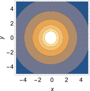
Figure 1: Iso-potential lines associated to (3.51), for $b=1$, $c=2$ and $a=0.2$. The left panel shows the charged cylinder creating the field (central circle), together with a zoom of the $\phi$ map. The right panel shows the iso-potentials on a larger scale. Long-distance isotropy becomes apparent.

For completeness Fig. 1 shows the contour plot of $\phi(x,y)$ for the lowest order mode ($b=1$). It appears that the iso-potential lines become more and more isotropic, moving away from the charged cylinder shown in red on the left hand panel.

Here also, an ansatz of the form (3.49) yields a family of new solutions. We now discuss the most salient feature of these generalized solutions.

III.4.3 Mode mixing

In the light of our previous cylindrical/planar mapping remark, we will discuss here the planar case only, keeping in mind the correspondence between exponential pattern screening for planes, and algebraic pattern screening for cylinders (with an exponent related to the period of the periodic charge/potential pattern on the surface of the cylinder).

We generalize Eq. (3.35) into

$$Y_{1}(z)\,=\,z+a_{1}e^{-b_{1}z}+a_{2}e^{-b_{2}z},\qquad Y_{2}(z)=1$$ (3.52)

with $b_{1},b_{2}>0$. This lead to the potential $\phi(\widetilde{x},\widetilde{y})$ given by

$$\phi = -2\ln\left[c+\widetilde{x}+a_{1}e^{-b_{1}\widetilde{x}}\cos(b_{1}\widetilde{y})+a_{2}e^{-b_{2}\widetilde{x}}\cos(b_{2}\widetilde{y})\right]$$ (3.53)

$$+\ln\left\{1-2a_{1}b_{1}e^{-b_{1}\widetilde{x}}\cos(b_{1}\widetilde{y})-2a_{2}b_{2}e^{-b_{2}\widetilde{x}}\cos(b_{2}\widetilde{y})\right.$$

$$+(a_{1}b_{1})^{2}e^{-2b_{1}\widetilde{x}}+(a_{2}b_{2})^{2}e^{-2b_{2}\widetilde{x}}$$

$$+2\left.a_{1}b_{1}a_{2}b_{2}\,e^{-(b_{1}+b_{2})\widetilde{x}}\,\cos[(b_{1}-b_{2})\widetilde{y}]\right\}$$

and a more complex “two-mode” pattern on the plane at $x=0$ than in section III.4.1. We see that considering two modes with periods (in coordinate $\tilde{y}$) $2\pi/b_{1}$ and $2\pi/b_{2}$ in the function ansatz (3.52) implies in the potential solution (3.53) the corresponding decay lengths (in coordinate $\tilde{x}$) $1/b_{1}$ and $1/b_{2}$, respectively. Yet, the contrubution dominating at long distances is not necessarily the one having the largest period since there is a contribution with period $2\pi/|b_{1}-b_{2}|$, which may possibly be the largest one, with a small decay length $1/(b_{1}+b_{2})$. From these results, we can surmise that the Fourier transform of a given charge pattern on the plate will not allow to identify the long-distance electrostatic signature of the plate, by searching for the mode with smallest wave number. As outlined above, these results immediately transpose to the cylindrical geometry, upon changing terms like $e^{-(b_{i})\widetilde{x}}$ into $(\widetilde{r})^{-b_{i}}$.

III.5 A perturbative solution of the Liouville equation

We next propose a perturbative treatment of the 2D Liouville equation around the full solution of the uniform surface charge density by considering its periodic modulations with infinitesimally small amplitudes. This will confirm the conclusions of the previous sections.

Let us add to the uniform potential solution (3.5) an infinitesimal perturbation $\epsilon f(\widetilde{x},\widetilde{y})$ with $\epsilon\ll 1$:

$$\phi(\widetilde{x},\widetilde{y})=-2\ln(c+\widetilde{x})+\epsilon f(\widetilde{x},\widetilde{y}).$$ (3.54)

The parameter $c>0$ will be related to the surface charge density subsequently. Inserting this ansatz into the 2D Poisson-Boltzmann/Liouville equation (3.10) and expanding all functions up to terms linear in the small parameter $\epsilon$, the function $f(x,y)$ must obey

$$\frac{\partial^{2}f}{\partial\widetilde{x}^{2}}+\frac{\partial^{2}f}{\partial\widetilde{y}^{2}}=\frac{2}{(c+\widetilde{x})^{2}}f.$$ (3.55)

Using separation of variables

$$f(\widetilde{x},\widetilde{y})=\varphi(\widetilde{x})\psi(\widetilde{y})$$ (3.56)

the functions $\varphi$ and $\psi$ fulfill the second-degree ordinary differential equation

$$\frac{1}{\varphi}\frac{d^{2}\varphi}{d\widetilde{x}^{2}}=b^{2}+\frac{2}{(c+\widetilde{x})^{2}},\qquad\frac{1}{\psi}\frac{d^{2}\psi}{d\widetilde{y}^{2}}=-b^{2}$$ (3.57)

with $b$ a free positive real number. The solution for $\psi$ is

$$\psi=\cos\left(b\widetilde{y}\right),$$ (3.58)

where the prefactor is set to unity for simplicity. The solution for $\varphi$ reads

$$\varphi=e^{-b\widetilde{x}}\left(b+\frac{1}{c+\widetilde{x}}\right).$$ (3.59)

The total potential

$$\phi=-2\ln(c+\widetilde{x})+\epsilon e^{-b\widetilde{x}}\left(b+\frac{1}{c+\widetilde{x}}\right)\cos(b\widetilde{y})$$ (3.60)

generates the surface charge density $\sigma(\widetilde{y})$ via the relation (3.11),

$$4\pi\ell_{\rm B}^{2}\sigma(\widetilde{y})=\frac{2}{c}+\epsilon\left(b^{2}+\frac{b}{c}+\frac{1}{c^{2}}\right)\cos(b\widetilde{y}).$$ (3.61)

It is readily checked that the small $a$ limit of the non perturbative solution provided by Eq. (3.38), coincides with Eq. (3.60).

Averaging equation (3.61) along the $\widetilde{y}$ axis over the period $2\pi/b$ implies that the parameter $c$ is related directly to the mean value of the surface charge density,

$$c=\frac{1}{2\pi\ell_{\rm B}^{2}\langle\sigma\rangle}.$$ (3.62)

To leading order in the smallness parameter $\epsilon$, the contact relation takes the form

$$n(0,\tilde{y})=\left[1-\epsilon b^{2}c\cos(b\tilde{y})\right]2\pi\ell_{\rm B}\sigma^{2}(\tilde{y}),$$ (3.63)

with the prefactor smaller than 1 as was expected.

We recover here the same conclusion as above, although limited to a perturbative treatment: the corrugation (i.e. the $y$-dependence) of the surface charge $\sigma e$ is exponentially suppressed upon increasing the distance $x$ to the plate, see Eq. (3.60) for the spatial dependence of the potential. Besides, the connection between the period $2\pi/b$ of the pattern, and the pattern screening length $1/b$ is clearly apparent.

IV Situations with added salt

Now we turn to situations where a planar macroion is immersed in an infinite sea of electrolyte, playing the role of a salt reservoir and setting the Debye length $\kappa^{-1}$.

Let $x,y$ coordinates be measured in units of $1/\kappa$,

$$\widetilde{x}=\kappa x,\qquad\widetilde{y}=\kappa y.$$ (4.1)

We are looking for regular potential solutions of the 2D version of the PB equation (2.16)

$$\frac{\partial^{2}\phi}{\partial\widetilde{x}^{2}}+\frac{\partial^{2}\phi}{\partial\widetilde{y}^{2}}=\sinh\phi,$$ (4.2)

the so-called 2D sinh-Gordon equation which is related to the better known 2D sine-Gordon equation via the transformation $\phi\to i\phi$. The surface charge density, which in general depends on $\widetilde{y}$, is again determined by the boundary condition

$$\frac{\partial\phi(\widetilde{x},\widetilde{y})}{\partial\widetilde{x}}\Big{|}_{\widetilde{x}=0}=-\frac{4\pi\ell_{\rm B}\sigma(\widetilde{y})}{\kappa}.$$ (4.3)

For completeness, we recall in Appendix C the main results for a homogeneously charged plate.

IV.1 2D Debye-Hückel solutions

Unlike in the no-salt case, we start with a perturbative Debye-Hückel (DH) treatment. Within the DH approach, the linearization of $\sinh\phi\sim\phi$ in (4.2) leads to the Helmholtz equation

$$\frac{\partial^{2}\phi_{\rm DH}}{\partial\widetilde{x}^{2}}+\frac{\partial^{2}\phi_{\rm DH}}{\partial\widetilde{y}^{2}}=\phi_{\rm DH}.$$ (4.4)

Its solutions, which depend on both coordinates, can be obtained by using separation of variables:

$$\phi_{\rm DH}=\varphi(\widetilde{x})\psi(\widetilde{y}),$$ (4.5)

where $\varphi$ and $\psi$ obey the second-degree ordinary equations

$$\frac{1}{\varphi}\frac{d^{2}\varphi}{d\widetilde{x}^{2}}=\frac{1}{1-\gamma^{2}},\qquad\frac{1}{\psi}\frac{d^{2}\psi}{d\widetilde{y}^{2}}=-\frac{\gamma^{2}}{1-\gamma^{2}},$$ (4.6)

with the real parameter $\gamma\in(0,1)$. In particular,

$$\phi_{\rm DH}=c_{1}\sin\left(\frac{\gamma\widetilde{y}}{\sqrt{1-\gamma^{2}}}\right)\exp\left(-\frac{\widetilde{x}}{\sqrt{1-\gamma^{2}}}\right),$$ (4.7)

where $c_{1}$ is real. This electrostatic potential is periodic along the $\widetilde{y}$-axis, with period (in units of the Debye length)

$${\cal P}(\gamma)=\frac{2\pi\sqrt{1-\gamma^{2}}}{\gamma}.$$ (4.8)

Comparing the result (4.7) with the uniform DH solution (C.10), it is clear that any periodic modulation along the $\widetilde{y}$-axis implies a faster exponential decay in the $\widetilde{x}$ direction. The decay rate along the $x$-axis depends on the period of the sine function along the $y$-axis: larger period means smaller $\gamma$ and consequently slower decay (the decay length is bounded from above by the Debye length, a value that is reached for an infinite period along $y$, i.e. with $\gamma=0$ rque102 ). The form of the corresponding surface charge density follows from the boundary condition (4.3):

$$\frac{4\pi\ell_{\rm B}\sigma_{\rm DH}(\widetilde{y})}{\kappa}=\frac{c_{1}}{\sqrt{1-\gamma^{2}}}\sin\left(\frac{\gamma\widetilde{y}}{\sqrt{1-\gamma^{2}}}\right).$$ (4.9)

Since the Helmholtz equation (4.4) is linear, any superposition of particular solutions also is a solution:

$$\phi_{\rm DH} = c\exp\left(-\widetilde{x}\right)+\sum_{n}c_{n}\sin\left(\frac{\gamma_{n}\widetilde{y}}{\sqrt{1-\gamma_{n}^{2}}}\right)$$ (4.10)

$$\times\exp\left(-\frac{\widetilde{x}}{\sqrt{1-\gamma_{n}^{2}}}\right),$$

where the parameters $\gamma_{1}<\gamma_{2}<\ldots<\gamma_{N}$ are from the interval $(0,1)$, $c$ is any real constant and $c_{1},\ldots,c_{N}$ are nonzero real constants. The corresponding surface charge density $\sigma_{\rm DH}$ is given by

$$\frac{4\pi\ell_{\rm B}\sigma_{\rm DH}(\widetilde{y})}{\kappa}=c+\sum_{n}\frac{c_{n}}{\sqrt{1-\gamma_{n}^{2}}}\sin\left(\frac{\gamma_{n}\widetilde{y}}{\sqrt{1-\gamma_{n}^{2}}}\right).$$ (4.11)

Note that

$$\frac{4\pi\ell_{\rm B}\langle\sigma_{\rm DH}\rangle}{\kappa}=c.$$ (4.12)

If $c\neq 0$, the dominant term at large distances in (4.10) is the one with the uniform surface charge density equal to $\langle\sigma_{\rm DH}\rangle$. If $c=0$, i.e. $\langle\sigma_{\rm DH}\rangle=0$, the dominant term corresponds to the smallest $\gamma_{1}$, i.e. to the largest period (4.8).

The extension of the DH formalism to general profiles of the surface charge varying along both $y$ and $z$ axis is straightforward. On a general ground a Fourier mode of wave number $k$ for the charge pattern on the plate results in a far-field decay with a screening rate $\sqrt{1+k^{2}}$. Hence, the smallest $k$ (the smallest $\gamma$) provides the mode that extends the furthest into the bulk.

Since the potential $\phi$ in the 2D Poisson equation (4.2) vanishes at $\widetilde{x}\to\infty$, this equation can be linearized in the asymptotic region (large $\widetilde{x}$) and its general solution is of type (4.10), which allows to define renormalized coefficients, following the uniform plate approach. It is seen that the asymptotic potential is generically of the form $\exp(-\widetilde{x})$, meaning that the surface corrugation is washed out with $\widetilde{x}$, and that the asymptotic decay is set by the Debye length. At finite distance from the wall, surface charge modulations with various periods influence each other due to the nonlinearity of the sinh-Gordon equation. One may surmise here that the above generic scenario holds provided $\langle\sigma\rangle\neq 0$. The situation with $\langle\sigma\rangle=0$ is more subtle to analyze; an explicit case is worked out below. Finally, we emphasize that the phenomenon of saturation can be documented on exactly solvable cases; it corresponds to the fact that a divergent surface charge may nevertheless yield a finite potential at all points outside the charged body creating the field TT03 .

IV.2 Soliton solutions of 2D Poisson-Boltzmann/sinh-Gordon equation

All solutions of the 2D equation (4.2) are available due to the existence of Bäcklund transformation which reduces the second-order differential equation (4.2) to a couple of the first-order ones Rogers82 . The simplest soliton one-particle solutions, formulated standardly within the related 2D sine-Gordon theory, is used to generate via the Bäcklund transformation solutions with higher number of soliton “particles” Hirota92 ; Samaj13 .

The one-soliton solution has the form

$$\phi=2\ln\left\{\frac{\exp{\left[(\widetilde{x}+a)/\sqrt{1+\gamma^{2}}\right]}+\xi\exp{\left[-\gamma(\widetilde{y}+b)/\sqrt{1+\gamma^{2}}\right]}}{\exp{\left[(\widetilde{x}+a)/\sqrt{1+\gamma^{2}}\right]}-\xi\exp{\left[-\gamma(\widetilde{y}+b)/\sqrt{1+\gamma^{2}}\right]}}\right\},$$ (4.13)

where the coordinate shifts $a$ and $b$ are arbitrary (they only renormalize $\xi>0$) and the parameter $\gamma$ is real. There always exist negative values of $\widetilde{y}$ such that the denominator of the fraction under logarithm is equal to 0 or negative, which is physically unacceptable. To put it differently, Eq. (4.13) leads to physically reasonable solution in the upper quadrant only ($x\geq 0;y\geq 0$) and we do not dwell further on its properties. The only exception is when $\gamma=0$ for which (4.13) (with $a=0$) reduces to the uniformly charged plate solution (C.4).

We turn to the two-soliton solutions of the sinh-Gordon equation, that can be written as a formal generalization of the one-soliton result (4.13):

$$\phi(\tilde{x},\tilde{y})=2\ln\left[\frac{f(\widetilde{x})+g(\widetilde{y})}{f(\widetilde{x})-g(\widetilde{y})}\right].$$ (4.14)

The function $g(\tilde{y})$ should obey the differential equation

$$[g^{\prime}(\widetilde{y})]^{2}=Ag^{4}(\widetilde{y})-Bg^{2}(\widetilde{y})+C$$ (4.15)

with some as-yet undetermined real coefficients $A$, $B$ and $C$. The derivation of this equation with respect to $\widetilde{y}$ yields

$$g^{\prime\prime}(\widetilde{y})=2Ag^{3}(\widetilde{y})-Bg(\widetilde{y}).$$ (4.16)

Similarly, the function $f(\widetilde{x})$ satisfies the equation

$$[f^{\prime}(\widetilde{x})]^{2}=A^{\prime}f^{4}(\widetilde{x})-B^{\prime}f^{2}(\widetilde{x})+C^{\prime}$$ (4.17)

with some other real coefficients $A^{\prime}$, $B^{\prime}$ and $C^{\prime}$. As before, differentiating this equation with respect to $\widetilde{x}$ yields

$$f^{\prime\prime}(\widetilde{x})=2A^{\prime}f^{3}(\widetilde{x})-B^{\prime}f(\widetilde{x}).$$ (4.18)

Inserting the ansatz (4.14) into the sinh-Gordon equation (4.2) and using the relations (4.15)–(4.18) it can be shown that the functions $f(x)$ and $g(y)$ provide the solution of (4.2) if

$$A^{\prime}=-A,\qquad B^{\prime}=-(B+1),\qquad C^{\prime}=-C.$$ (4.19)

For a special choice of the coefficients

$$A=A^{\prime}=0,\qquad B=C=\frac{\gamma^{2}}{1-\gamma^{2}},$$

$$B^{\prime}=-\frac{1}{1-\gamma^{2}},\qquad C^{\prime}=-\frac{\gamma^{2}}{1-\gamma^{2}}$$ (4.20)

with the real parameter

$$0<\gamma<1,$$ (4.21)

the $f$ and $g$ functions are obtained as follows

$$f=\gamma\cosh\left(\frac{\widetilde{x}}{\sqrt{1-\gamma^{2}}}+a\right),\quad g=\sin\left(\frac{\gamma\widetilde{y}}{\sqrt{1-\gamma^{2}}}\right),$$ (4.22)

where $a$ is a real positive number. The resulting potential is

$$\phi=2\ln\left[\frac{\gamma\cosh\left(\frac{\widetilde{x}}{\sqrt{1-\gamma^{2}}}+a\right)+\sin\left(\frac{\gamma\widetilde{y}}{\sqrt{1-\gamma^{2}}}\right)}{\gamma\cosh\left(\frac{\widetilde{x}}{\sqrt{1-\gamma^{2}}}+a\right)-\sin\left(\frac{\gamma\widetilde{y}}{\sqrt{1-\gamma^{2}}}\right)}\right].$$ (4.23)

Keeping in mind that $x\geq 0$, the inequality

$$\gamma\cosh a>1$$ (4.24)

must hold in order to avoid the singularity in $\phi$. This inequality is equivalent to

$$a>a_{c}=\ln\left[\frac{1}{\gamma}\left(1+\sqrt{1-\gamma^{2}}\right)\right].$$ (4.25)

Using the boundary condition (4.3), the surface charge density is given by

$$\sigma=\frac{\kappa}{\pi\ell_{\rm B}}\frac{\gamma\sinh a}{\sqrt{1-\gamma^{2}}}\frac{\sin\left(\frac{\gamma\widetilde{y}}{\sqrt{1-\gamma^{2}}}\right)}{\gamma^{2}\cosh^{2}a-\sin^{2}\left(\frac{\gamma\widetilde{y}}{\sqrt{1-\gamma^{2}}}\right)}.$$ (4.26)

This function is periodic with the period ${\cal P}(\gamma)$ given by (4.8). The parameter $a$, constrained by the inequality (4.24), controls the amplitude of oscillations which is enhanced when $\gamma\cosh a$ is close to 1. Since $\sigma(\widetilde{y})=-\sigma(-\widetilde{y})$, the mean value of the surface charge density over the period vanishes,

$$\langle\sigma\rangle=0.$$ (4.27)

The behavior of the surface charge is shown in Fig. 2. For $a=a_{c}$, the surface charge is divergent at specific points. Yet, the electrostatic potential is regular for $x>0$, see Fig. 3. For $x=0$, the potential exhibits a diverging tip at the points where $\sigma$ diverges.

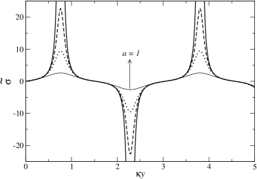
Figure 2: Plot of the dimensionless surface charge $\widetilde{\sigma}=\pi l_{B}\sigma/\kappa$ stemming from Eq. (4.26) for $\gamma=0.9$, as a function of $\widetilde{y}=\kappa y$. For this situation, the period of the charge pattern is ${\cal P}\simeq 3.04$. The thick continuous, dashed, dotted and thin continuous curves are for $a=a_{c}$, $a=0.52$, $0.6$ and 1, respectively. The critical $a$ associated to the constraint (4.25) is $a_{c}\simeq 0.467$, it leads to a locally diverging surface charge.

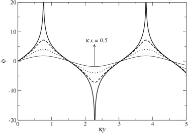
Figure 3: Electrostatic potential profiles as given by (4.23). The plot shows the $y$ dependence (parallel to the charged plate), for different distances to the plates: $\gamma=0.9$ as in Fig. 2 with $a=a_{c}$. The thick continuous, dashed, dotted and thin continuous curves are for $\widetilde{x}=\kappa x=0$, $0.05$, $0.2$ and $0.5$, respectively.

The reduced potential decays at large distances from the wall as

$$\phi(\widetilde{x},\widetilde{y})\mathop{\sim}_{\widetilde{x}\to\infty}\frac{8e^{-a}}{\gamma}\sin\left(\frac{\gamma\widetilde{y}}{\sqrt{1-\gamma^{2}}}\right)\exp\left(-\frac{\widetilde{x}}{\sqrt{1-\gamma^{2}}}\right).$$ (4.28)

It is seen that the surface charge density (4.26), which is periodic function of $\widetilde{y}$ with a relatively complicated Fourier series, implies at asymptotic distances from the wall the potential of the DH form (4.7) as was expected. The exact relationship to the DH theory can be documented by considering the limit $a\to\infty$ of the surface charge density (4.26):

$$\frac{4\pi\ell_{\rm B}\sigma(\widetilde{y})}{\kappa}\sim\frac{8}{\gamma}\frac{1}{\sqrt{1-\gamma^{2}}}e^{-a}\sin\left(\frac{\gamma\widetilde{y}}{\sqrt{1-\gamma^{2}}}\right),$$ (4.29)

which corresponds to the DH surface charge density (4.9) with $c_{1}=8e^{-a}/\gamma\ll 1$. The DH potential (4.7) is then equivalent to our asymptotic potential (4.28). Eq. (4.28) indicates that the asymptotic screening length is (in units of the Debye length) $\ell=\sqrt{1-\gamma^{2}}$. For the $\gamma$-parameter of Fig. 3, this yields a length $\ell\simeq 0.43$. This is compatible with the data shown in Fig. 3, where it is seen that for $\widetilde{x}=\kappa x=0.5$ already, $\phi$ exhibits significantly reduced oscillations. The linear response regime, where $\phi$ is everywhere smaller than 1, is reached for $\widetilde{x}>0.76$.

The particle species densities, given by $n_{\pm}=(n/2)e^{\mp\phi}$, read as

$$n_{+} = \frac{n}{2}\left[\frac{\gamma\cosh\left(\frac{\widetilde{x}}{\sqrt{1-\gamma^{2}}}+a\right)-\sin\left(\frac{\gamma\widetilde{y}}{\sqrt{1-\gamma^{2}}}\right)}{\gamma\cosh\left(\frac{\widetilde{x}}{\sqrt{1-\gamma^{2}}}+a\right)+\sin\left(\frac{\gamma\widetilde{y}}{\sqrt{1-\gamma^{2}}}\right)}\right]^{2},$$

$$n_{-} = \frac{n}{2}\left[\frac{\gamma\cosh\left(\frac{\widetilde{x}}{\sqrt{1-\gamma^{2}}}+a\right)+\sin\left(\frac{\gamma\widetilde{y}}{\sqrt{1-\gamma^{2}}}\right)}{\gamma\cosh\left(\frac{\widetilde{x}}{\sqrt{1-\gamma^{2}}}+a\right)-\sin\left(\frac{\gamma\widetilde{y}}{\sqrt{1-\gamma^{2}}}\right)}\right]^{2}.$$

At each distance from the wall $\widetilde{x}$, the particle species densities fulfill the equality $n_{+}(\widetilde{x},\widetilde{y})=n_{-}(\widetilde{x},-\widetilde{y})$, so the integral over the charge density vanishes, i.e.

$$\langle\rho(\widetilde{x})\rangle=0\quad\mbox{for each $\widetilde{x}\in[0,\infty)$.}$$ (4.31)

For large distances from the wall, the particle charge density decays as

$$\rho(\widetilde{x},\widetilde{y})\mathop{\sim}_{\widetilde{x}\to\infty}\frac{8ene^{-a}}{\gamma}\sin\left(\frac{\gamma\widetilde{y}}{\sqrt{1-\gamma^{2}}}\right)\exp\left(-\frac{\widetilde{x}}{\sqrt{1-\gamma^{2}}}\right).$$ (4.32)

The total particle density at the wall $n(0,\widetilde{y})\equiv n_{+}(0,\widetilde{y})+n_{-}(0,\widetilde{y})$ satisfies a local relation of type (2.31)

$$n(0,\widetilde{y})-n\,=\,\frac{1-\gamma^{2}}{\tanh^{2}a}\,\,2\pi\ell_{\rm B}\sigma^{2}(\widetilde{y}).$$ (4.33)

Using the restriction on the $a$ parameter (4.25) it can be shown that the prefactor

$$\frac{1-\gamma^{2}}{\tanh^{2}a}<1,$$ (4.34)

in agreement with the general theory presented in Sec. II. It is easy to show that the contact relations (2.26) and (2.28) are satisfied. The mean value (over the period) of the total particle density as the function of the distance from the wall $\widetilde{x}$ behaves as

$$\frac{\langle n(\widetilde{x})\rangle}{n}-1=\frac{4\left[\gamma\cosh\left(\frac{\widetilde{x}}{\sqrt{1-\gamma^{2}}}+a\right)\right]}{\left\{\left[\gamma\cosh\left(\frac{\widetilde{x}}{\sqrt{1-\gamma^{2}}}+a\right)\right]^{2}-1\right\}^{3/2}}.$$ (4.35)

At asymptotically large distances $\widetilde{x}$, one has

$$\frac{\langle n(\widetilde{x})\rangle}{n}-1\mathop{\sim}_{\widetilde{x}\to\infty}\frac{16e^{-2a}}{\gamma^{2}}\exp\left(-\frac{2\widetilde{x}}{\sqrt{1-\gamma^{2}}}\right),$$ (4.36)

or a more detailed asymptotic relation

$$\frac{n(\widetilde{x},\widetilde{y})}{n}-1 \displaystyle{\mathop{\sim}_{\widetilde{x}\to\infty}} \frac{32e^{-2a}}{\gamma^{2}}\sin^{2}\left(\frac{\gamma\widetilde{y}}{\sqrt{1-\gamma^{2}}}\right)$$ (4.37)

$$\times\exp\left(-\frac{2\widetilde{x}}{\sqrt{1-\gamma^{2}}}\right).$$

Comparing this formula with its analogue for the particle charge density (4.32), we see that the approach of the particle number to its bulk value is faster by a factor $2$ in the exponential.

Finally, let the amplitude of the surface charge density (4.26) go to infinity, i.e. $\gamma\cosh a=1$, which defines $a_{c}$. Equivalently,

$$e^{a_{c}}=\frac{1}{\gamma}\left(1+\sqrt{1-\gamma^{2}}\right).$$ (4.38)

Considering this relation in the asymptotic decay of the potential (4.28), the prefactor

$$\frac{8\,e^{-a}}{\gamma}=\frac{8}{1+\sqrt{1-\gamma^{2}}}$$ (4.39)

becomes finite which is evidence for the saturation phenomenon TT03 . Note that the saturated prefactor depends on $\gamma$ and its value ranges between $4$ for $\gamma\to 1$ and $8$ for $\gamma\to 0$. This leads to the remark that the situation leading to the most enhanced large-distance potential is when $\gamma\to 0$, meaning that the period of the charge pattern diverges. We have already met earlier this feature. Figure 4 illustrates saturation of the electrostatic signature, for the different charge patterns presented in Fig. 2. It is observed that for $a\leq 0.6$, the potential at the chosen distance from the plate ($\widetilde{x}=0.5$), depends quite weakly on $a$, while the surface charge evolves from strongly modulated at $a=0.6$, to locally divergent at $a=a_{c}$. Besides, the divergent surface charge for $a=a_{c}$ yields a well behaved potential. The potential for $a=1$ is distinct from the other three, since it corresponds to too weak modulation.

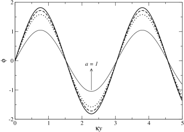
Figure 4: Electrostatic potential at a fixed distance from the wall, $\widetilde{x}=0.5$, for the various charge patterns shown in Fig. 2. The thick continuous, dashed, dotted and thin continuous curves are for $a=a_{c}$, $a=0.52$, $0.6$ and 1 respectively, with $a_{c}\simeq 0.467$.

A natural next step is to proceed to many-soliton solutions, using e.g. a simplified Hirota’s method Wazwaz12 . The problem is that the transition from the sine-Gordon to sinh-Gordon theories via the transformation $\phi\to i\phi$ converts regular solutions to unacceptable singular ones.

IV.3 A perturbative solution of the Poisson-Boltzmann/sinh-Gordon equation

The above non-perturbative solution of the 2D Poisson-Boltzmann equation for the potential (4.23) contains two independent parameters $\gamma\in(0,1)$ and $a$, constrained by (4.24). By varying these parameters one can obtain a number of various forms of the corresponding surface charge density (4.26), however all forms have the common property that $\langle\sigma\rangle=0$. In analogy with the 2D Liouville equation in Sec. III.5, we propose in what follows a perturbative treatment of the 2D problem around the full solution of the uniform surface charge density, by considering a small periodic modulation. We recall that in the standard DH approach the whole potential is taken as a small quantity in which case the sinh function can be linearized. The present treatment thus differs from the linear response derived in section IV.1.

Let us add to the uniform potential solution (C.4) an infinitesimal perturbation $\epsilon f(\widetilde{x},\widetilde{y})$ with $\epsilon\ll 1$:

$$\phi(\widetilde{x},\widetilde{y})=\phi_{0}(\widetilde{x})+\epsilon f(\widetilde{x},\widetilde{y}),\qquad\phi_{0}=2\ln\left(\frac{e^{\widetilde{x}}+\xi}{e^{\widetilde{x}}-\xi}\right).$$ (4.40)

The parameter $\xi$ is as-yet unspecified, and will be related to the surface charge density. Inserting this ansatz into the 2D sinh-Gordon equation (4.2), the function $f(x,y)$ must obey

$$\frac{\partial^{2}f}{\partial\widetilde{x}^{2}}+\frac{\partial^{2}f}{\partial\widetilde{y}^{2}}=f\cosh\phi_{0},$$ (4.41)

where

$$\cosh\phi_{0}(\widetilde{x}) = \frac{1}{2}\left[\left(\frac{e^{\widetilde{x}}+\xi}{e^{\widetilde{x}}-\xi}\right)^{2}+\left(\frac{e^{\widetilde{x}}-\xi}{e^{\widetilde{x}}+\xi}\right)^{2}\right]$$ (4.42)

$$= 1+\frac{8\xi^{2}e^{-2\widetilde{x}}}{\left(1-\xi^{2}e^{-2\widetilde{x}}\right)^{2}}.$$

Note that Eq. (4.41) is in fact the linearized DH version of the sinh-Gordon equation with the position-dependent $\kappa(\widetilde{x})=\sqrt{4\pi\ell_{\rm B}n(\widetilde{x})}$, where $n(\widetilde{x})$ is the standard PB total particle density for the uniformly charged plate.

Using separation of variables

$$f(\widetilde{x},\widetilde{y})=\varphi(\widetilde{x})\psi(\widetilde{y})$$ (4.43)

in Eq. (4.41), the $\varphi$ and $\psi$ functions must obey

$$\frac{1}{\varphi}\frac{d^{2}\varphi}{d\widetilde{x}^{2}}=\frac{1}{1-\gamma^{2}}+\frac{8\xi^{2}e^{-2\widetilde{x}}}{\left(1-\xi^{2}e^{-2\widetilde{x}}\right)^{2}},\qquad\frac{1}{\psi}\frac{d^{2}\psi}{d\widetilde{y}^{2}}=-\frac{\gamma^{2}}{1-\gamma^{2}}.$$ (4.44)

The solution for $\psi$ reads as

$$\psi=\sin\left(\frac{\gamma\widetilde{y}}{\sqrt{1-\gamma^{2}}}\right).$$ (4.45)

The solution for $\varphi$ is searched as a series

$$\varphi=e^{-\widetilde{x}/\sqrt{1-\gamma^{2}}}\sum_{n=0}^{\infty}c_{n}\xi^{2n}e^{-2n\widetilde{x}}.$$ (4.46)

Inserting this series into Eq. (4.44) implies a recurrent scheme for the coefficient

$$\frac{1}{2}n\left(n+\frac{1}{\sqrt{1-\gamma^{2}}}\right)c_{n}=\sum_{j=0}^{n-1}(n-j)c_{j},$$ (4.47)

where $n=1,2,\ldots$ and $c_{0}$ is free. It is straightforward to verify that the constant series

$$c_{n}=\frac{2\sqrt{1-\gamma^{2}}}{1+\sqrt{1-\gamma^{2}}}c_{0}$$ (4.48)

solves the recursion (4.47). Setting $c_{0}=1$, $\varphi$ is found to be

$$\varphi=e^{-\widetilde{x}/\sqrt{1-\gamma^{2}}}\left(1+\frac{2\sqrt{1-\gamma^{2}}}{1+\sqrt{1-\gamma^{2}}}\frac{\xi^{2}e^{-2\widetilde{x}}}{1-\xi^{2}e^{-2\widetilde{x}}}\right).$$ (4.49)

The total potential reads as

$$\phi = 2\ln\left(\frac{e^{\widetilde{x}}+\xi}{e^{\widetilde{x}}-\xi}\right)+\epsilon\sin\left(\frac{\gamma\widetilde{y}}{\sqrt{1-\gamma^{2}}}\right)e^{-\widetilde{x}/\sqrt{1-\gamma^{2}}}$$ (4.50)

$$\times\left(1+\frac{2\sqrt{1-\gamma^{2}}}{1+\sqrt{1-\gamma^{2}}}\frac{\xi^{2}e^{-2\widetilde{x}}}{1-\xi^{2}e^{-2\widetilde{x}}}\right).$$

The corresponding surface charge density $\sigma(\widetilde{y})$, generated via the relation (4.3), takes the form

$$\frac{4\pi\ell_{\rm B}\sigma(\widetilde{y})}{\kappa} = \frac{4\xi}{1-\xi^{2}}+\epsilon\sin\left(\frac{\gamma\widetilde{y}}{\sqrt{1-\gamma^{2}}}\right)$$

$$\times\frac{(1+\xi^{2})^{2}+\sqrt{1-\gamma^{2}}(1-\xi^{4})-2\gamma^{2}\xi^{2}}{\sqrt{1-\gamma^{2}}(1+\sqrt{1-\gamma^{2}})(1-\xi^{2})^{2}}.$$

Averaging this equation over the period leads to

$$\frac{4\pi\ell_{\rm B}\langle\sigma\rangle}{\kappa}\equiv a=\frac{4\xi}{1-\xi^{2}},$$ (4.52)

where $\xi$ as the function of $a$ is expressed in Eq. (C.5).

It stands to reason that in the limit $\langle\sigma\rangle\to 0$ $(\xi\to 0)$ our equations (4.50) and (LABEL:sigmafinal) reduce to their DH counterparts (4.7) and (4.9). The conclusions of previous sections on screening lengths and periodicity are unaltered.

V Conclusion

This article was devoted to deriving new analytical solutions to the Poisson-Boltzmann theory, that describes equilibrium electric double-layers around charged macromolecules. We have addressed deionized situations (counterions only, also known as salt-free) and others when the double-layer is in equilibrium with a bulk of salt, playing the role of a reservoir. Previously known solutions pertain to uniformly charged macromolecules, and we focused on models with inhomogeneous surface charge densities, referred to as patterns. In doing so, generic effects of screening emerge.

The no-salt case was solved in Sec. III, taking advantage of known results for the 2D Liouville equation (3.10) for the mean (reduced) potential $\phi$. All solutions of this equation are known, see relations (3.13)-(3.16). Once a solution for $\phi$ is chosen, the corresponding surface charge density is generated in an inverse way from the boundary condition (3.11). The problem with these solutions is that the great majority of them have singularities (divergencies) in the particle region $\Lambda$ and/or the nonvanishing derivative of $\phi$ with respect to $x$ at $x\to\infty$ which corresponds to unphysical non-neutral charge systems. A generic feature in the no-salt case is that a periodic charge pattern (with non-vanishing mean) is screened exponentially in the planar case. This may be surprising since the counterion density, a measure of charge screening, decays algebraically, as the inverse squared distance to the plate. One should thus distinguish charge screening (the recovery of a neutral system at large distance), from heterogeneity screening (the loss of charge/potential patterning). The situation for a charged cylinder differs, in the sense that pattern screening becomes algebraic. This can be rationalized by the planar to cylindrical mapping presented in section III.3, which highlights the Cartesian/cylindrical coordinates correspondence $\widetilde{x}\leftrightarrow\ln\widetilde{r}$, $\widetilde{y}\leftrightarrow\varphi$. More precisely, a charge pattern on the cylinder with angular period $2\pi/b$ where $b$ is some integer, has a signature in the potential that decays as the inverse power-law $\widetilde{r}^{-b}$. This is superimposed to the global decay of potential/density away from the charged cylinder, that reduces at large distance to that of a cylinder without any charge pattern.

For system with added salt, our main results pertain to planar interfaces with periodic charge patterns. The planar to cylindrical correspondence is lost. This discussion is developed in Sec. IV. The linearized DH approach, based on the Helmholtz equation (4.4), provides the modulated solutions of type (4.7) where the decay rate along the $x$-axis is directly related to the period of the sine function along the $y$-axis. The nonlinear Poisson-Boltzmann approach is associated with the 2D sinh-Gordon equation (4.2). This equation is integrable and possesses a number of many-soliton solutions, but practically all solutions suffer from singularities within the space $\Lambda$ occupied by the particles. An exception is represented by the 2-soliton solution for the potential (4.23) which implies the periodic surface charge density (4.26) with zero mean. It is interesting that this relatively complicated solution provides the local contact relation (4.33). The phenomenon of saturation TT03 ; Trizac02 is documented on this model: increasing the amplitude of periodic oscillations of the surface charge density to infinity implies the asymptotic decay of the potential (4.28) with the finite prefactor (4.39). To understand also the systems with a nonzero mean of the surface charge density, we constructed in Sec. IV.3 a perturbative treatment of the 2D sinh-Gordon equation in infinitesimal periodic modulations of the uniform surface charge density, in close analogy with the 2D Liouville equation. Moreover, we have found that the signature of surface charge pattern extends all the more into the bulk electrolyte as the associated period of the pattern is large. The connection between the period $\cal P$ of the charge pattern and the screening length $\ell$ reads

$$\frac{\ell}{\cal P}\,=\,\frac{1}{\sqrt{\kappa^{2}{\cal P}^{2}+(2\pi)^{2}}}.$$ (5.1)

For small period $\kappa{\cal P}\ll 1$, we have $\ell\sim{\cal P}/(2\pi)$. Increasing $\cal P$, the screening length increases as well, and saturates to $\kappa^{-1}$ for large periods.

A general analysis of the statistical quantities at the wall contact was the subject of Sec. II. Using the pressure tensor, we have derived the integral constraint for the local pressure given by Eqs. (II.3) and (2.25) which relates the surface charge density and the statistical quantities at the wall contact, namely the particle density and the parallel component of the electric field. This integral constraint was verified to be true for every exactly solvable model. The inequality (2.30) consequently applies. An important feature for the no-salt case is the confirmation of the enhancement of the counterion density at the wall in comparison with the uniform case. It is possible that the established upper bound of the mean contact particle density in Eq. (3.47) is of general validity.

Variations of the surface charge density studied in this paper were restricted to one direction, so that the proposed solutions depend on two coordinates, and not three. It would be useful to have exactly solved models for more general profiles of the surface charge varying along both $y$ and $z$ axis, but this requires the solution of 3D versions of the Liouville or sinh-Gordon equations. Although a 3D Bäcklund transformation has already been proposed for the Liouville equation Leibbrandt80 ; Huang06 , the exact solutions seem out of reach.

Finally, while we focussed on one macroion features, it would be relevant to study macroion-macroion interactions within this formalism, and to compare to known results. It was indeed shown recently that nano-patterned surfaces exhibit an interaction force that strongly depends on the alignement between charged domains, and of the domain size Bakhshandeh18 ; comment2001 . Work along these lines is in progress.

Appendix A Rederivation of the integral pressure relation

We show here how to recover Eqs. (II.3) and (2.25) by direct use of the PB equation (2.11). We consider the counterion only situation. Multiplying the PB equation by $\partial\phi/\partial x$ and integrating over $x$ from $0$ to $\infty$, we obtain

$$4\pi\ell_{\rm B}n(0,y,z)-\frac{1}{2}\left(\frac{\partial\phi}{\partial x}\right)^{2}\Big{|}_{x=0}\phantom{aaaaa}$$

$$+\int_{0}^{\infty}dx\frac{\partial\phi}{\partial x}\frac{\partial^{2}\phi}{\partial y^{2}}+\int_{0}^{\infty}dx\frac{\partial\phi}{\partial x}\frac{\partial^{2}\phi}{\partial z^{2}}=0.$$ (A.1)

Next we use the boundary condition (2.12) at $x=0$, divide the above equation by $4\pi\ell_{\rm B}$ and finally integrate it over $y$ and $z$ from $-\infty$ to $\infty$, to get

$$\int_{-\infty}^{\infty}dy\int_{-\infty}^{\infty}dz\left[n(0,y,z)-2\pi\ell_{\rm B}\sigma^{2}(y,z)\right]\phantom{aaaaa}$$

$$+\frac{1}{4\pi\ell_{\rm B}}\int_{0}^{\infty}dx\int_{-\infty}^{\infty}dy\int_{-\infty}^{\infty}dz\frac{\partial\phi}{\partial x}\frac{\partial^{2}\phi}{\partial y^{2}}$$

$$+\frac{1}{4\pi\ell_{\rm B}}\int_{0}^{\infty}dx\int_{-\infty}^{\infty}dy\int_{-\infty}^{\infty}dz\frac{\partial\phi}{\partial x}\frac{\partial^{2}\phi}{\partial z^{2}}=0.$$

Using integrations by parts with the neglection of boundary terms at infinity in the $(x,y)$-subspace, we get the following equivalence of integrals:

$$\int_{-\infty}^{\infty}dy\left(\frac{\partial\phi}{\partial y}\right)^{2}\Big{|}_{x=0} = -\int_{-\infty}^{\infty}dy\int_{0}^{\infty}dx\frac{\partial}{\partial x}\left(\frac{\partial\phi}{\partial y}\right)^{2}$$

$$= -2\int_{0}^{\infty}dx\int_{-\infty}^{\infty}dy\frac{\partial^{2}\phi}{\partial x\partial y}\frac{\partial\phi}{\partial y}$$

$$= 2\int_{0}^{\infty}dx\int_{-\infty}^{\infty}dy\frac{\partial\phi}{\partial x}\frac{\partial^{2}\phi}{\partial y^{2}}.$$

Proceeding similarly in the $(x,z)$-subspace results in

$$\int_{-\infty}^{\infty}dz\left(\frac{\partial\phi}{\partial z}\right)^{2}\Big{|}_{x=0}=2\int_{0}^{\infty}dx\int_{-\infty}^{\infty}dz\frac{\partial\phi}{\partial x}\frac{\partial^{2}\phi}{\partial z^{2}}.$$ (A.4)

Inserting the last two integral equalities into (A), we arrive at the contact relation given by Eqs. (II.3) and (2.25).

Appendix B Derivation of non-neutral solutions

Choosing in (3.18) the parameters

$$c_{1}=\frac{1}{2c},\quad c_{2}=-\frac{c}{2}+\frac{a^{2}}{2c},\quad\alpha=\frac{a}{2c},\quad\beta=0,$$ (B.1)

which fulfill the constraint (3.19), we obtain

$$\phi=-2\ln\left\{\frac{1}{2c}\left[(\widetilde{x}+a)^{2}+\widetilde{y}^{2}\right]-\frac{c}{2}\right\}.$$ (B.2)

To ensure that the expression under logarithm is positive at any point in $\Lambda$, it is necessary that

$$0<c<a.$$ (B.3)

The boundary condition (3.11) yields the surface charge density on the plate at $x=0$:

$$\sigma=\frac{1}{\pi\ell_{B}^{2}}\frac{a}{a^{2}-c^{2}+\widetilde{y}^{2}}.$$ (B.4)

It is maximal at $\widetilde{y}=0$ and monotonously decays to zero for $\widetilde{y}\to\pm\infty$. The corresponding density profile follows from Eq. (3.12),

$$n=\frac{2c^{2}}{\pi\ell_{B}^{3}}\frac{1}{\left[(\widetilde{x}+a)^{2}-c^{2}+\widetilde{y}^{2}\right]^{2}}.$$ (B.5)

There exists a non-trivial local relation between the particle density at the wall and the surface charge density

$$n(0,\widetilde{y})=\left(\frac{c}{a}\right)^{2}2\pi\ell_{\rm B}\sigma^{2}(\widetilde{y})$$ (B.6)

which is of type (2.31) with the prefactor $(c/a)^{2}<1$, in agreement with the theory developed in Sec. II. The integral contact relation, given by Eqs. (2.26) and (2.27), is easily verified to be valid. For a finite value of the $\widetilde{y}$-coordinate and at asymptotically large distances $\widetilde{x}$ from the wall, we have

$$n(x,y)\mathop{\sim}_{x\to\infty}\frac{2c^{2}\ell_{\rm B}}{\pi}\frac{1}{x^{4}},$$ (B.7)

which is thus $y$-independent. This asymptotic relation is partially nonuniversal since it contains the surface charge parameter $c$, however it does not involve the parameter $a$. Since

$$(-e)\ell_{\rm B}^{2}\int_{-\infty}^{\infty}{\rm d}\widetilde{y}\int_{0}^{\infty}{\rm d}\widetilde{x}n(\widetilde{x},\widetilde{y})=\frac{(-e)}{\ell_{\rm B}}\left(\frac{a}{\sqrt{a^{2}-c^{2}}}-1\right)$$ (B.8)

and

$$\qquad e\ell_{\rm B}\int_{-\infty}^{\infty}{\rm d}\widetilde{y}\sigma(\widetilde{y})=\frac{e}{\ell_{\rm B}}\frac{a}{\sqrt{a^{2}-c^{2}}},$$ (B.9)

one particle (per unit length in the $z$ direction) is evaporated in the sense of the Manning-Oosawa condensation Oosawa68 ; Manning69 ; BuOr06 ; Juan .

Other solutions are given by the choices

$$Y_{1}(z)=z^{n}\quad(n=2,3,\ldots),\qquad Y_{2}(z)=1.$$ (B.10)

They possess qualitatively the same features as the $n=1$ case. In particular, the asymptotic decay of the density profile is of the type $n(x,y)\sim x^{-2-2n}$ for $x\to\infty$. We do not dwell further on this family for the following reason. While we started the analysis in planar geometry, the very form of the solutions obtained (see Eq. (B.2)), together with the intrusion of a Manning-like evaporation phenomenon, indicates that we are actually contemplating the potential created by a charged cylinder, and that cylindrical coordinates with radial variable $\widetilde{r}=\sqrt{(\widetilde{x}+a)^{2}+\widetilde{y}^{2}}$ would simplify the formulation, for the angular dependence is here absent. The resulting charged cylinder problem is thus isotropic (homogeneous surface charge), and the charge inhomogeneity obtained with Cartesian coordinates is thus artificial, stemming from an inappropriate choice of coordinates. Besides, the solution (B.2) actually corresponds to a non-neutral system where, beyond the unavoidable Manning evaporation Oosawa68 ; Manning69 ; BuOr06 ; Juan , there are too few counterions to neutralize the cylinder charge.

All these solutions (including $n=1$) correspond to “initially non-neutral” cylindrical geometry configurations, since the potential decays too fast at infinity; we do not have a $-2\ln r$ but a $-2(1+n)\ln r$. What is meant here is that beyond the unavoidable Manning evaporation phenomenon, the solutions here correspond to a non-neutral system enclosed in a concentric Wigner-Seitz cylinder, the radius of which is sent to infinity rque200 .

Appendix C Homogeneous surface charge density for systems with salt

Introducing the dimensionless coordinate $\widetilde{x}=\kappa x$, the one-dimensional version of the PB equation (2.16) is written as

$$\frac{d^{2}\phi}{d\widetilde{x}^{2}}=\sinh\phi$$ (C.1)

and the boundary condition (2.12) at $\widetilde{x}=0$ takes the form

$$-\frac{\partial\phi}{\partial\widetilde{x}}\Big{|}_{\widetilde{x}=0}=\frac{4\pi\ell_{\rm B}\sigma}{\kappa}\equiv a.$$ (C.2)

The potential $\phi$ is positive and its derivative $\phi^{\prime}(\widetilde{x})$ negative for all $\widetilde{x}\geq 0$ (we are dealing with a positively charged surface). Multiplying the PB equation (C.1) by $\phi^{\prime}(\widetilde{x})$, it can be simply integrated to the one Andelman06

$$\phi^{\prime}(\widetilde{x})=-2\sinh\frac{\phi(\widetilde{x})}{2},$$ (C.3)

which has the explicit solution

$$\phi=2\ln\left(\frac{e^{\widetilde{x}}+\xi}{e^{\widetilde{x}}-\xi}\right),\qquad a=\frac{4\xi}{1-\xi^{2}}.$$ (C.4)

In order to ensure the positivity of $\phi$, the parameter $\xi$ is chosen as the positive root of the quadratic equation,

$$\xi=\frac{-2+\sqrt{4+a^{2}}}{a}.$$ (C.5)

Its value is from the interval $(0,1)$, namely $\xi\to 0$ for $a\to 0$ (small $\sigma$) and $\xi\to 1$ for $a\to\infty$ (large $\sigma$).

At large distances from the wall, $\phi$ decays to zero exponentially,

$$\phi\mathop{\sim}_{\widetilde{x}\to\infty}4\xi e^{-\widetilde{x}},$$ (C.6)

as it should be for dense Coulomb systems. The species densities

$$n_{\pm}(\widetilde{x})=\frac{n}{2}e^{\mp\phi(\widetilde{x})}=\frac{n}{2}\left(\frac{1\mp\xi e^{-\widetilde{x}}}{1\pm\xi e^{-\widetilde{x}}}\right)^{2}$$ (C.7)

also decay exponentially to their bulk value $n/2$, from below for coions and from above for counterions. The total particle density at the wall

$$n(0)=n_{+}(0)+n_{-}(0)=n\cosh\phi(0)=n+2\pi\ell_{\rm B}\sigma^{2}$$ (C.8)

fulfills the contact theorem (2.23).

The Debye-Hückel (DH) approach is based on the linearization of the PB equation (C.1),

$$\frac{d^{2}\phi_{\rm DH}}{d\widetilde{x}^{2}}=\phi_{\rm DH}.$$ (C.9)

The regular solution of this equation with the boundary condition (C.2) reads as

$$\phi_{\rm DH}=\frac{4\pi\ell_{\rm B}\sigma}{\kappa}\exp\left(-\widetilde{x}\right).$$ (C.10)

Also the original nonlinear PB equation (C.1) can be linearized at $\widetilde{x}\to\infty$ since $\phi$ is small, and the general solution of the linearized equation is analogous to the DH one (C.9), up to a $\sigma$-dependent prefactor,

$$\phi\mathop{\sim}_{\widetilde{x}\to\infty}A(\sigma)\exp\left(-\widetilde{x}\right).$$ (C.11)

In analogy with the DH solution (C.10), the prefactor $A(\sigma)$ defines an effective (or renormalized) surface charge density $\sigma_{\rm eff}$ via the relation Alexander84 ; Diehl01 ; Trizac02 ; Samaj15

$$A(\sigma)=\frac{4\pi\ell_{\rm B}\sigma_{\rm eff}}{\kappa}.$$ (C.12)

The explicit nonlinear solution (C.4), when expanded in $\exp(-\widetilde{x})$, implies

$$\frac{4\pi\ell_{\rm B}\sigma_{\rm eff}}{\kappa}=4\xi.$$ (C.13)

For small $\sigma$, $\xi\sim a/4$ and $\sigma_{\rm eff}\sim\sigma$. In the limit $\sigma\to\infty$, $\xi\to 1$ and $\sigma_{\rm eff}$ saturates to a finite value given by

$$\frac{\pi\ell_{\rm B}\sigma_{\rm eff}^{\rm sat}}{\kappa}=1.$$ (C.14)

References

- (1) D. Andelman, Introduction to Electrostatics in Soft and Biological Matter, in Soft Condensed Matter Physics in Molecular and Cell Biology, edited by W. C. K. Poon and D. Andelman (Taylor& Francis, New York, 2006).
- (2) T. Palberg, M. Medebach, N. Garbow, M. Evers, A. B. Fontecha, H. Reiber, and E. Bartsch, J. Phys.: Condens. Matter 16, S4039 (2004).
- (3) Ph. Attard, D. J. Mitchell, and B. W. Ninham, J. Chem Phys. 88, 4987 (1988); 89, 4358 (1988).
- (4) R. Podgornik, J. Phys. A 23, 275 (1990).
- (5) R. R. Netz and H. Orland, Eur. Phys. J. E 1, 203 (2000).
- (6) A. G. Moreira and R. R. Netz, Europhys. Lett. 52, 705 (2000); Phys. Rev. Lett. 87, 078301 (2001).
- (7) R.R. Netz, Eur. Phys. J. E 5, 557 (2001).
- (8) A.G. Moreira and R.R. Netz, Eur. Phys. J. E 8, 33 (2002).
- (9) M. Kanduč and R. Podgornik, Eur. Phys. J. E 23, 265 (2007).
- (10) Y. S. Jho, M. Kanduč, A. Naji, R. Podgornik, M. W. Kim, and P. A. Pincus, Phys. Rev. Lett. 101, 188101 (2008).
- (11) M. Kanduč, M. Trulsson, A. Naji, Y. Burak, J. Forsman, and R. Podgornik, Phys. Rev. E 78, 061105 (2008).
- (12) L. Šamaj and E. Trizac, Phys. Rev. Lett. 106, 078301 (2011); Phys. Rev. E 84, 041401 (2011).
- (13) L. Šamaj, A. P. dos Santos, Y. Levin, and E. Trizac, Soft Matter 12, 8768 (2016).
- (14) L. Šamaj, M. Trulsson, and E. Trizac, Soft Matter 14, 4040 (2018).
- (15) G. L. Gouy, J. Phys. 9, 457 (1910).
- (16) D. L. Chapman, Philos. Mag. 25, 475 (1913).
- (17) Ph. Attard, Adv. Chem. Phys. 92, 1 (1996).
- (18) J. P. Hansen and H. Löwen, Annu. Rev. Phys. Chem. 51, 209 (2000).
- (19) Y. Levin, Rep. Prog. Phys. 65, 1577 (2002).
- (20) R. Messina, J. Phys.: Condens. Matter 21, 113102 (2009).
- (21) E. J. W. Verwey and J. Th. G. Overbeek, Theory of the Stability of Lyophobic Colloids (Elsevier, New York, 1948).
- (22) M. Polat and H. Polat, J. Colloid Interface Sci. 341, 178 (2009).
- (23) M. Dubois, T. Zemb, N. Fuller, R. P. Rand, and V. A. Pargesian, J. Chem. Phys. 108, 7855 (1998).
- (24) T. Alfrey Jr, P.W. Berg, and H. Morawetz, J Polym. Sci. 7, 543 (1951); R.M. Fuoss, A. Katchalsky, and S.F. Lifson, P. Natl. Acad. Sci. USA 37, 579 (1951).
- (25) J. Liouville, J. Math. 18, 71 (1853).
- (26) C. A. Tracy and H. Widom, Physica A 244, 402 (1997).
- (27) E. Trizac and G. Téllez, Phys. Rev. Lett. 96, 038302 (2006).
- (28) T. Shen and E. Trizac, Europhysics Letters 116, 18007 (2016).
- (29) S. Guilbaud, L. Salomé, N. Destainville, M. Manghi, and C. Tardin, Phys. Rev. Lett. 122, 028102 (2019).
- (30) J. Y. Walz, Adv. Colloid Interface Sci. 74, 119 (1998).
- (31) D. Y. C. Chan, J. Mitchell, and B. W. Ninham, J. Chem. Phys. 72, 5159 (1980).
- (32) R. Kjellander and S. Marčelja, J. Chem. Phys. 88, 7138 (1988).
- (33) O. Gonzalez-Amezcua, M. Hernandez-Contreras, and P. A. Pincus, Phys. Rev. E 64, 041603 (2001).
- (34) A. G. Moreira and R. R. Netz, EPL 57, 911 (2002).
- (35) D. B. Lukatsky, S. A. Safran, A. W. C. Lau, and P. A. Pincus, EPL 58, 785 (2002).
- (36) M. L. Henle, C. D. Santangelo, D. M. Patel, and P. A. Pincus, EPL 66, 284 (2004).
- (37) C. C. Fleck and R. R. Netz, EPL 70, 341 (2005).
- (38) D. B. Lukatsky and S. A. Safran, EPL 60, 629 (2002).
- (39) M. O. Khan, S. Petris, and D. Y. C. Chan, J. Chem. Phys. 122, 104705 (2005).
- (40) It was argued in Ref. Landy10 that in the weak coupling regime, counterion surface enhancement and pressure reduction can facilitate both overcharging and like-charge attraction. Studies of surfaces with quenched charge disorder in the strong coupling regime Naji05 ; Ghodrat15 ; Bakhshandeh15 indicate that the disorder-induced attraction between the charged surfaces can become much stronger than their van der Waals interaction.
- (41) D. Henderson and L. Blum, J. Chem. Phys. 69, 5441 (1978).
- (42) D. Henderson, L. Blum, and J. L. Lebowitz, J. Electroanal. Chem. 102, 315 (1979).
- (43) S. L. Carnie and D. Y. C. Chan, J. Chem. Phys. 74, 1293 (1981).
- (44) H. Wennerström, B. Jönsson, and P. Linse, J. Chem. Phys. 76, 4665 (1982).
- (45) L. Blum and D. Henderson, Statistical Mechanics of Electrolytes at Interfaces, in Fundamentals of Inhomogeneous Fluids, edited by D. Henderson (Dekker, New York, 1992), pp 239-276.
- (46) L. Blum, J. Stat. Phys. 75, 971 (1994).
- (47) E. Trizac and J.-P. Hansen, Phys. Rev. E 56, 3137 (1997).
- (48) J. P. Mallarino, G. Téllez, and E. Trizac, Mol. Phys. 113, 2409 (2015).
- (49) P. Malgaretti and M. Bier, Phys. Rev. E 97, 022102 (2018).
- (50) J. D. Jackson, Classical Electrodynamics, 3rd ed. (John Wiley, New York, 1998).
- (51) L. D. Landau and E. M. Lifschitz, Electrodynamics of Continuous Media (Pergamon Press, Oxford, 1984).
- (52) P. H. Chavanis, Eur. Phys. J. B 87, 81 (2014).
- (53) E. Picard, J. Math. 130, 243 (1898).
- (54) P. A. Clarkson and M. D. Kruskal, J. Math. Phys. 30, 2201 (1989).
- (55) O. P. Bhutani, M. H. M. Moussa, and K. Vijayakumar, Int. J. Engng. Sci. 32, 1965 (1994).
- (56) A. G. Popov, Dokl. Akad. Nauk 333, 440 (1993).
- (57) D. G. Crowdy, Int. J. Engng. Sci. 35, 141 (1997).
- (58) Y. Burak and H. Orland, Phys. Rev. E 73, 010501(R) (2006).
- (59) F. Oosawa, Biopolymers 6, 134 (1968).
- (60) G. Manning, J. Phys. Chem. 51, 924 (1969).
- (61) J.P. Mallarino, G. Tellez, and E. Trizac, J. Phys. Chem. B 117, 12702 (2013).
- (62) Note that while the period of charge modulation along the plate is arbitrary when compared to the Debye length, the screening length perpendicular to the plate is smaller, or at most equal to the Debye length.
- (63) G. Téllez and E. Trizac, Phys. Rev. E 68, 061401 (2003).
- (64) C. Rogers and W. F. Shadwick, Bäcklund Transformations and Their Applications (Academic Press, New York, 1982).
- (65) R. Hirota, Direct Methods in Soliton Theory (Cambridge University Press, Cambridge, 1992).
- (66) L. Šamaj and Z. Bajnok, Introduction to the Statistical Physics of Integrable Many-body Systems (Cambridge University Press, Cambridge, 2013).
- (67) A.-M. Wazwaz, J. Appl. Math. & Informatics 30, 925 (2012).
- (68) E. Trizac, L. Bocquet, and M. Aubouy, Phys. Rev. Lett. 89, 248301 (2002).
- (69) G. Leibbrandt, Lett. Math. Phys. 4, 317 (1980).
- (70) X. Huang and E. H. C. Chang, Int. J. Appl. Sci. Eng. 4, 215 (2006).
- (71) We note in passing that while it is possible to find solutions that behave in at large distances with , cases with are precluded since they correspond to a situation where all counterions would evaporate to infinity, by the Manning mechanism. Besides, as emphasized in the main text, the most interesting solutions behave at large distances as .
- (72) S. Alexander, P. M. Chaikin, P. Grant, G. J. Morales, and P. Pincus, J. Chem. Phys. 80, 5776 (1984).
- (73) A. Diehl, M. C. Barbosa, and Y. Levin, Europhys. Lett. 53, 86 (2001).
- (74) L. Šamaj and E. Trizac, J. Phys. A: Math. Theor. 48, 265003 (2015).
- (75) J. Landy, Phys. Rev. E 81, 011401 (2010).
- (76) A. Naji and R. Podgornik, Phys. Rev. E 72, 041402 (2005).
- (77) M. Ghodrat, A. Naji, H. Komaie-Moghaddam, and R. Podgornik, Soft Matter 11, 3441 (2015).
- (78) A. Bakhshandeh, A. P. dos Santos, A. Diehl, and Y. Levin, J. Chem Phys. 142, 194707 (2015).
- (79) A. Bakhshandeh, A. P. dos Santos, and Y. Levin, Soft Matter 14, 4081 (2018).
- (80) A comment is in order here, formulated in the planar case for simplicity. Starting from one of our solutions, one may compute the normal electric field at an arbitrary distance on a parallel plane, and infer from this the corresponding surface charge density. The potential outside the two plates will be unaffected and coincide with that of our initial single plate problem; also unaffected will be the total pressure, which has to be the same on both plates, and always vanishing in our case. This is a way to extend our one-plate results to two-plate interactions. Such a route, however, can be seen as somewhat artificial: we cannot choose the charge pattern on the second plate, and the net pressure will always be zero.