Storage or No Storage: Duopoly Competition Between Renewable Energy Suppliers in a Local Energy Market

Abstract

Renewable energy generations and energy storage are playing increasingly important roles in serving consumers in power systems. This paper studies the market competition between renewable energy suppliers with or without energy storage in a local energy market. The storage investment brings the benefits of stabilizing renewable energy suppliers’ outputs, but it also leads to substantial investment costs as well as some surprising changes in the market outcome. To study the equilibrium decisions of storage investment in the renewable energy suppliers’ competition, we model the interactions between suppliers and consumers using a three-stage game-theoretic model. In Stage I, at the beginning of the investment horizon (containing many days), suppliers decide whether to invest in storage. Once such decisions have been made (once), in the day-ahead market of each day, suppliers decide on their bidding prices and quantities in Stage II, based on which consumers decide the electricity quantity purchased from each supplier in Stage III. In the real-time market, a supplier is penalized if his actual generation falls short of his commitment. We characterize a price-quantity competition equilibrium of Stage II in the local energy market, and we further characterize a storage-investment equilibrium in Stage I incorporating electricity-selling revenue and storage cost. Counter-intuitively, we show that the uncertainty of renewable energy without storage investment can lead to higher supplier profits compared with the stable generations with storage investment due to the reduced market competition under random energy generation. Simulations further illustrate results due to the market competition. For example, a higher penalty for not meeting the commitment, a higher storage cost, or a lower consumer demand can sometimes increase a supplier’s profit. We also show that although storage investment can increase a supplier ’s profit, the first-mover supplier who invests in storage may benefit less than the free-rider competitor who chooses not to invest.

I Introduction

I-A Background and motivation

Renewable energy, as a clean and sustainable energy source, is playing an increasingly important role in power systems [2]. For example, from the year 2007 to 2017, the global installed capacity of solar panels has increased from 8 Gigawatts to 402 Gigawatts, and the wind power capacity has increased from 94 Gigawatts to 539 Gigawatts[2]. Compared with traditional larger-scale generators, renewable energy sources can be more spatially distributed across the power system, e.g., at the distribution level near residential consumers[2]. Due to the distributed nature of renewable energy generations, there has been growing interest in forming local energy markets for renewable energy suppliers and consumers to trade electricity at the distribution level [3]. Such local energy markets will allow consumers to purchase electricity from the least costly sources locally[4], and allow suppliers to compete in selling electricity directly to consumers (instead of dealing with the utility companies).

However, many types of renewable energy are inherently random, due to factors such as weather conditions that are difficult to predict and control. Under current multi-settlement energy market structures with day-ahead and real-time bidding rules (which are mostly designed for controllable generations)[5], renewable energy suppliers face a severe disadvantage in the competition by making forward commitment (in the day-ahead market) that they may not be able to deliver in real time. For example, suppliers are often subject to a penalty cost if their real-time delivery deviates from the commitment in the day-ahead market[6].

Energy storage has been considered as an important type of flexible resources for renewable energy suppliers to stabilize their outputs[7]. Investing in storage can potentially improve the renewable energy suppliers’ position in these energy markets. However, investing in storage incurs substantial investment costs. Furthermore, the return of storage investment depends on the outcome of the market, which in turn depends on how suppliers with or without storage compete for the demand. Therefore, it remains an open problem regarding whether competing renewable energy suppliers should invest in energy storage in the market competition and what economic benefits the storage can bring to the suppliers.

I-B Main results and contributions

In this paper, we formulate a three-stage game-theoretic model to study the market equilibrium for both storage investment as well as price and quantity bidding of competing renewable energy suppliers. In Stage I, at the beginning of the investment horizon, each supplier decides whether to invest in storage. We formulate a storage-investment game between two suppliers in Stage I, which is based on a bimatrix game to model suppliers’ storage-investment decisions for maximizing profits[8]. Given the storage-investment decisions in Stage I, competing suppliers decide the bidding price and bidding quantity in the (daily) local energy market in Stage II. We formulate a price-quantity competition game between suppliers using the Bertrand-Edgeworth model [9] (which models price competition with capacity constraints) in Stage II. Given suppliers’ bidding strategies, consumers decide the electricity quantity purchased from each supplier in Stage III. To the best of our knowledge, our work is the first to study the storage-investment equilibrium between competing renewable energy suppliers in the two-settlement energy market. This problem is quite nontrivial due to the penalty cost on the random generations of a general probability distribution.

By studying this three-stage model, we reveal a number of new and surprising insights that are against the prevailing wisdom in the literature on the renewable energy suppliers’ revenues in such a two-settlement market [6, 10] and on the economic benefits of storage supplementing in renewable energy sources [11, 12].

• First, the uncertainty of the renewable generation can be favorable to suppliers. Note that the prevailing wisdom is that storage investment (especially when the storage cost is low) will improve suppliers’ revenue by stabilizing their outputs [11, 12]. In contrast, we find that the opposite may be true when considering market competition. Specifically, without storage, suppliers with random generations always have strictly positive revenues when facing any positive consumer demand. However, if both suppliers invest in storage and stabilize their renewable outputs, their revenues reduce to zero once the consumer demand is below a threshold, which is due to the increased market competition after storage investment.

• Second, a higher penalty and a higher storage cost can also be favorable to the suppliers. Note that the common wisdom is that a higher penalty[10] and a higher storage cost[11] will decrease suppliers’ profit. However, when considering market competition, the opposite may be true. With a higher penalty for not meeting the commitment, renewable energy suppliers become more conservative in their bidding quantities, which can decrease market competition and increase their profits. Furthermore, a higher storage cost may change one supplier’s storage-investment decision, which can benefit the other supplier.

• Third, the first-mover supplier who invests in energy storage can be at the disadvantage in terms of profit increase, which is contrary to the first-mover advantage gained by early investment of resources or new technologies [13]. We find that although investing in storage can increase one supplier’s profit, it may benefit himself less than his competitor (who does not invest in storage). This is because the later mover becomes a free rider, who may benefit from the changed price equilibrium in the energy market (due to the storage investment of the other supplier) but does not need to bear the investment cost.

In addition to these surprising and new insights, a key technical contribution of our work is the solution to the game-theoretic model for the price-quantity competition, which involves a general penalty cost due to random generations of a general probability distribution. Note that such a price-quantity competition with the Bertrand-Edgeworth model has been studied in literature under quite different conditions from ours. The works in [14, 15, 16] studied a general competition between suppliers with strictly convex production costs. They focused on the analysis of pure strategy equilibrium without characterizing the mixed strategy equilibrium. The study in [17] characterized both pure and mixed strategy equilibrium between suppliers with deterministic supply. However, this work considered zero cost related to the production (i.e., no production cost or possible penalty cost). In electricity markets, the works in [18] and [19] also used Bertrand-Edgeworth model to analyze the competition among renewable energy suppliers with random generations. However, both [18] and [19] considered the suppliers’ electricity-selling competition in a single-settlement energy market, and suppliers deliver random generations in real time. These studies did not consider day-ahead bidding strategies and any deviation penalty cost. In particular, the two-settlement markets with deviation penalty have been essential for ensuring the reliable operation of power systems. Our work is the first to consider the two-settlement energy market, characterizing both pure and mixed strategy equilibrium based on the Bertrand-Edgeworth model. Such a setting is nontrivial due to the penalty cost caused by the suppliers’ random production of a general probability distribution.

The remainder of the paper is organized as follows. First, we introduce the system model in Section II, as well as the three-stage game-theoretic formulation between suppliers and consumers in Section III. Then, we solve the three-stage problem through backward induction. We first characterize the consumers’ optimal purchase decision of Stage III in Section IV. Then, we characterize the price-quantity equilibrium of Stage II and the storage-investment equilibrium of Stage I in Sections V and VI, respectively. We propose a probability-based method to compute the storage capacity in Section VII. Furthermore, in Section IX, we extend some of the theoretical results and insights from the duopoly case to the oligopoly case. Finally, we present the simulation results in Section VIII and conclude this paper in Section X.

II System Model

We consider a local energy market at the distribution level as shown in Figure 1. Consumers can purchase energy from both the main grid and local renewable energy suppliers. To achieve a positive revenue, the renewable energy suppliers (simply called suppliers in the rest of the paper) need to set their prices no greater than the grid price, and they will compete for the market share. Furthermore, suppliers can choose to invest in energy storage to stabilize their renewable outputs and reduce the uncertainty in their delivery. Next, we will introduce the detailed models of timescales, suppliers and consumers, and characterize their interactions in the two-settlement local energy market.

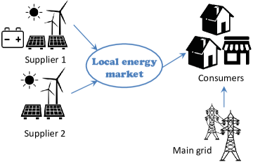
Figure 1: System structure.

II-A Timescale

We consider two timescales of decision-making. One is the investment horizon $\mathcal{D}=\{1,2,...,D_{s}\}$ of $D_{s}$ days (e.g., $D_{s}$ corresponding to the total number of days for the storage investment horizon). Suppliers can decide (once) whether to invest in energy storage at the beginning of the investment horizon. The investment horizon is divided into many operational horizons (many days), and each $d\in\mathcal{D}$ corresponds to the daily operation of the energy market, consisting of many time slots $\mathcal{T}=\{1,2,...,T\}$ (e.g., 24 hours of each day). In the day-ahead market on day $d-1$, suppliers decide the electricity price and quantity to consumers for each hour $t\in\mathcal{T}$ of the next day $d\in\mathcal{D}$. We will introduce the market structure in detail later in Section II.D.

II-B Suppliers

In Sections IV-VI, we focus on the duopoly case of two suppliers in our analysis. Later in Section IX, we further generalize to the oligopoly case with more than two suppliers. The reason for focusing on the duopoly case is twofold. First, our work focuses on a local energy market that is much smaller than a traditional wholesale energy market. The number of suppliers serving one local area is also expected to be limited [20], compared with thousands of suppliers in the wholesale energy market [21]. In such a small local energy market, a few large suppliers may dominate the market[22]. Second, we consider two suppliers for analytical tractability, which is without losing key insights and can effectively capture the impact of competition among suppliers considering the storage investment. For example, we show that in the duopoly case, the uncertainty of renewable generation can be beneficial to suppliers. Such an insight is still valid in the oligopoly case.

We denote $\mathcal{I}=\{1,2\}$ as the set of two suppliers. For hour $t$ of day $d$, the renewable output of supplier $i\in\mathcal{I}$ is denoted as a random variable $X_{i}^{d,t}$, which is bounded in $[0,\bar{X}_{i}^{d,t}]$. We assume that the random generation $X_{i}^{d,t}$ has a continuous cumulative distribution function (CDF) $F_{i}^{d,t}$ with the probability density function (PDF) $f_{i}^{d,t}$. The distribution of wind or solar power can be characterized using the historical data, which is known to the renewable energy suppliers. As renewables usually have extremely low marginal production costs compared with traditional generators, we assume zero marginal production costs for the suppliers[18] [19].

II-C Consumers

We consider the aggregate consumer population, and we denote the total consumer demand at hour $t$ of day $d$ as $D^{d,t}>0$. Note that consumers in one local area usually face the same electricity price from the same utility. Thus, if the local market’s electricity price is lower than the grid price, all the consumers will first purchase electricity from local suppliers. From the perspective of suppliers, they only care about the total demand of consumers and how much electricity they can sell to consumers.

Furthermore, our work conforms to the current energy market practice that suppliers make decisions in the day-ahead market based on the predicted demand. Thus, for the demand $D^{d,t}$, we consider it as a deterministic (predicted) demand in our model. Since the electricity demand is usually inelastic [5], we also assume the following.

Assumption 1.

Consumers’ demand is perfectly inelastic in the electricity price.

Consumers must purchase their demand $D^{d,t}$ either from the main grid (at a fixed unit price $P_{g}$) or from the local renewable suppliers (with prices to be discussed later).

II-D Two-settlement local energy market

We consider a two-settlement local energy market, which consists of a day-ahead market and a real-time market[5]. In such an energy market, suppliers have market power and can strategically decide their selling prices. Consumers have the flexibility to choose suppliers by comparing prices [4]. We explain the two-settlement energy market in detail as follows.

• In the day-ahead market on day $d-1$ (e.g., suppliers’ bids are cleared around 12:30pm of day $d-1$, one day ahead of the delivery day $d$[25]), supplier $i\in\mathcal{I}$ decides the bidding price $p_{i}^{d,t}$ and the bidding quantity $y_{i}^{d,t}$ for each future hour $t\in\mathcal{T}$ of the delivery day $d$. Based on suppliers’ bidding strategies, consumers decide the electricity quantity $x_{i}^{d,t}~{}(\leq y_{i}^{d,t})$ purchased from supplier $i$. Supplier $i$ will get the revenue of $p_{i}^{d,t}x_{i}^{d,t}$ in the day-ahead market by committing the delivery quantity $x_{i}^{d,t}$ to consumers. Thus, the day-ahead market is cleared through matching supply and demand. Any excessive demand from the consumers will be satisfied through energy purchase from the main grid.

• In the real-time market at each hour on the next day $d$, if supplier $i$’s actual generation falls short of the committed quantity $x_{i}^{d,t}$ (i.e., $x_{i}^{d,t}>X_{i}^{d,t}$), he needs to pay the penalty $\lambda(x_{i}^{d,t}-X_{i}^{d,t})$ in the real-time market, which is proportional to the shortfall with a unit penalty price $\lambda$. For the consumers, although suppliers may not deliver the committed electricity to them, the shortage part can be still satisfied by the system operator using reserve resources. The cost of reserve resources can be covered by the penalty cost on the suppliers.

Note that the suppliers and consumers make decisions only in the day-ahead market. No active decisions are made in the real-time market, but there may be penalty cost on the delivery shortage.

To facilitate the analysis, we further make several assumptions of this local energy market as follows. First, for the excessive amount of generations (i.e., $x_{i}^{d,t}<X_{i}^{d,t}$), we assume the following.

Assumption 2.

Suppliers can curtail any excessive renewable energy generation (beyond any specific given level).

Assumption 2 implies that we do not need to consider the possible penalty or reward on the excessive renewable generations in real time.

Second, the local energy market is much smaller compared with the wholesale energy market. Thus, the suppliers are usually small and hence may focus on serving local consumers. It is less likely for them to trade in the wholesale energy market. This is summarized in the following assumption.

Assumption 3.

Suppliers only participate in the local energy market and serve local consumers. They do not participate in the wholesale energy market.

Third, for the bidding price ${p_{i}}$ and penalty price $\lambda$, we impose the following bounds.

Assumption 4.

Each supplier $i$’s bidding price $p_{i}$ has a cap $\bar{p}$ that satisfies $p_{i}\leq\bar{p}<P_{g}$.

Assumption 5.

The penalty price satisfies $\lambda>\bar{p}$.

Assumption 4 is without loss of generality, since no supplier will bid a price higher than $P_{g}$; otherwise, consumers will purchase from the main grid. Assumption 5 ensures that the penalty is high enough to discourage suppliers from bidding higher quantities beyond their capability. Note that price cap $\bar{p}$ and the penalty $\lambda$ are exogenous fixed parameters in our model. Next, we introduce how suppliers invest in the energy storage to stabilize their outputs.

II-E Storage investment

Each supplier decides whether to invest in storage at the beginning of the investment horizon. We denote supplier $i$’s storage-investment decision variable as $\varphi_{i}$, where $\varphi_{i}=1$ means investing in storage and $\varphi_{i}=0$ means not investing. If supplier $i$ invests in storage, we assume the following.

Assumption 6.

The with-storage supplier will utilize the storage to completely smooth out his power output at the mean value of renewable generations.

Thus, supplier $i$ with the renewable generation $X_{i}^{d,t}$ will charge and discharge his storage to stabilize the power output at the mean value $\mathbb{E}[X_{i}^{d,t}]$. The charge and discharge power $CD_{i}^{d,t}$ is as follows.

$$CD_{i}^{d,t}=X_{i}^{d,t}-\mathbb{E}[X_{i}^{d,t}],$$ (1)

where $CD_{i}^{d,t}>0$ means charging the storage and $CD_{i}^{d,t}<0$ means discharging the storage. Note that $\mathbb{E}_{X_{i}^{d,t}}[CD_{i}^{d,t}]=0$, which implies the long-term average power that the suppliers need to charge or discharge his storage is zero. Next, we introduce how to characterize the storage capacity and the storage cost.

First, based on the charge and discharge random variable $CD_{i}^{d,t}$, we propose a simple yet effective probability-based method to characterize the storage capacity $S_{i}$ using historical data of renewable generation $X_{i}^{d,t}$. In particular, we set a probability threshold, and then aim to find a minimum storage capacity $S_{i}$ such that the energy level in the storage exceeds the capacity with a probability no greater than the probability threshold. We will explain this methodology in Section VII.

Second, we calculate the storage cost of suppliers over the investment horizon (scaled into one hour) as $C_{i}=c_{i}\kappa_{i}S_{i}$, where $c_{i}$ is the unit capacity cost over the investment horizon and $\kappa_{i}$ is the scaling factor that scales the investment cost over years to one hour. The factor $\kappa_{i}$ is calculated as follows. We first calculate the present value of an annuity (a series of equal annual cash flows) with the annual interest rate $r_{i}$ (e.g., $r_{i}=5\%$), and then we divide the annuity equally to each hour. This leads to the formulation of the factor $\kappa_{i}$ as follows [27].

$$\kappa_{i}=\frac{r_{i}(1+r_{i})^{y_{i}}}{(1+r_{i})^{y_{i}}-1}\cdot\frac{1}{Y_{d}},$$ (2)

where $y_{i}$ is the number of years over the investment horizon (e.g., $y_{i}=15$ for Li-ion battery that can last for 15 years), and $Y_{d}$ is the total hours in one year (e.g., $Y_{d}=365\times 24$).

Therefore, given the parameter $c_{i}$ and $\kappa_{i}$ as well as the probability distribution of random generation, the storage capacity and storage cost can be regarded as the fixed values for the supplier who invests in storage. Note that a higher storage capacity leads to a higher storage investment cost, which can further affect the storage-investment decisions in the suppliers’ competition. Next, in the Section III, we will introduce the three-stage model between suppliers and consumers in detail.

III Three-stage game-theoretic model

We build a three-stage model between suppliers and consumers. In Stage I, at the beginning of the investment horizon, each supplier decides whether to invest in storage. In the day-ahead energy market, for each hour of the next day, suppliers decide the bidding prices and quantities in Stage II, and consumers make the purchase decision in Stage III. Next, we first introduce the types of renewable-generation distributions for computing suppliers’ electricity-selling revenues over the investment horizon, and then we explain the three stages respectively in detail.

III-A Type of renewable-generation distributions

We cluster the distribution of renewable generation into several types. Note that suppliers’ revenues depend on the distribution of renewable generations. We use historical data of renewable energy to model the generation distribution. Specifically, for the renewable generations at hour $t$ of all the days over the investment horizon, we cluster the empirical distribution into $M$ types, e.g., $M=12$ for 12 months considering the seasonal effect. In this case, each type $m\in\mathcal{M}=\{1,2,\ldots,M\}$ occurs with a probability $\rho^{m}=\frac{1}{12}$ considering 12 months. We use the data of renewable energy of all days in month $m$ at hour $t$ to approximate the distribution of renewable generation at hour $t$ for all the days in this month $m$. Then, to study the interactions between consumers and suppliers in the local energy market, we will assume that the renewable generation of day $d$ follows a random type (month) $m$, uniformly chosen from $m\in\mathcal{M}$. For notation convenience, we replace all the superscripts $d,t$ into $m,t$.

III-B The three-stage model

We illustrate the three-stage model between suppliers and consumers in Figure 2.

• Stage I: at the beginning of the investment horizon, each supplier $i\in\{1,2\}$ decides the storage-investment decisions $\varphi_{i}\in\{0,1\}$.

• Stage II: in the day-ahead market, for each hour $t$ of the next day, each supplier $i$ decides his bidding price $p_{i}^{m,t}$ and bidding quantity $y_{i}^{m,t}$ based on suppliers’ storage-investment decisions, assuming that the renewable-generation distribution is of month $m$.

• Stage III: in the day-ahead market, for each hour $t$ of the next day, consumers decide the electricity quantity $x_{i}^{m,t}$ purchased from each supplier $i$ based on each supplier’s bidding price and quantity, assuming that the renewable-generation distribution is of month $m$.

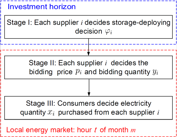
Figure 2: Three-stage model.

This three-stage problem is a dynamic game. The solution concept of a dynamic game is known as Subgame Perfect Equilibrium, which can be derived through backward induction[28]. Therefore, in the following, we will explain the three stages in detail in the order of Stage III, Stage II, and Stage I, respectively.

III-B1 Stage III

At hour $t$ of month $m$, given the bidding price $(p_{1}^{m,t},p_{2}^{m,t})$ and bidding quantity $(y_{1}^{m,t},y_{2}^{m,t})$ of both suppliers in Stage II, consumers decide the electricity quantity $(x_{1}^{m,t},x_{2}^{m,t})$ purchased from supplier 1 and supplier 2, respectively. The objective of consumers is to maximize the cost saving of purchasing energy from local suppliers compared with purchasing from the main grid only. We denote such cost saving as follows:

$$\pi_{c}^{m,t}(x_{1}^{m,t},x_{2}^{m,t})=(P_{g}-p_{1}^{m,t})x_{1}^{m,t}+(P_{g}-p_{2}^{m,t})x_{2}^{m,t}.$$ (3)

Recall that we model the collective purchase decision of the entire consumer population together. Consumers must satisfy their demand either from the local energy market or from the main grid (at the fixed price $P_{g}$). The total cost of satisfying the entire demand by the main grid is fixed. Therefore, minimizing the total energy cost is equivalent to maximizing the cost savings in the local energy market. We present consumers’ optimal purchase problem as follows.

Stage III: Consumers’ Cost Saving Maximization Problem

$$\max_{x_{1}^{m,t},x_{2}^{m,t}}~{} (P_{g}-p_{1}^{m,t})x_{1}^{m,t}+(P_{g}-p_{2}^{m,t})x_{2}^{m,t},$$ (4a)

s.t. $$x_{1}^{m,t}+x_{2}^{m,t}\leq D^{m,t},$$ (4b)

$$0\leq x_{i}^{m,t}\leq y_{i}^{m,t},i=1,2.~{}$$ (4c)

Constraint (4b) states that the total purchased quantity $x_{1}^{m,t}+x_{2}^{m,t}$ is no greater than the demand $D^{m,t}$. Constraints (4c) states that the quantity purchased from supplier $i$ is no greater than his bidding quantity $y_{i}^{m,t}$. This problem is a linear programming and can be easily solved, which we show in Section IV. We denote the optimal solution to Problem (4) as a function of suppliers’ bidding prices and quantities $(\bm{p}^{m,t},\bm{y}^{m,t})$, i.e., $x_{i}^{m,t*}(\bm{p}^{m,t},\bm{y}^{m,t}),~{}\forall i=1,2$, where $\bm{p}^{m,t}=(p_{1}^{m,t},p_{2}^{m,t})$ and $\bm{y}^{m,t}=(y_{1}^{m,t},y_{2}^{m,t})$.

III-B2 Stage II

Given the storage-investment decision $\bm{\varphi}=(\varphi_{1},\varphi_{2})$ in Stage I, both suppliers decide the bidding price $\bm{p}^{m,t}$ and bidding quantity $\bm{y}^{m,t}$ to maximize their revenues in Stage II. We denote supplier $i$’s electricity-selling revenue as $\pi_{i}^{R,m,t}$, which consists of two parts: the commitment revenue $p_{i}^{m,t}x_{i}^{m,t*}(\bm{p}^{m,t},\bm{y}^{m,t})$ from committing the delivery quantity in the day-ahead market, and the penalty cost in the real-time market. Supplier $i$ who invests in storage (i.e., $\varphi_{i}=1$) will be penalized if the committed quantity $x_{i}^{m,t*}(\bm{p}^{m,t},\bm{y}^{m,t})$ is larger than his stable generation $\mathbb{E}[{X}_{i}^{m,t}]$. Supplier $i$ who does not invest in storage (i.e., $\varphi_{i}=0$) will be penalized if the commitment $x_{i}^{m,t*}(\bm{p}^{m,t},\bm{y}^{m,t})$ is larger than his actual random generation ${X}_{i}^{m,t}$.

Note that the decisions of two suppliers are coupled with each other. If one supplier bids a lower quantity or a higher price, it is highly possible that consumers will purchase more electricity from the other supplier. We formulate a price-quantity competition game between suppliers given storage-investment decisions $\bm{\varphi}$ as follows.

Stage II: Price-quantity competition game

• Players: supplier $i\in\{1,2\}$.

• Strategies: bidding quantity $y_{i}^{m,t}\geq 0$ and bidding price $p_{i}^{m,t}\in[0,\bar{p}]$ of each supplier $i$.

• Payoffs: supplier $i$’s revenue at hour $t$ of month $m$ is

  $$\pi_{i}^{R,m,t}\left({p}_{i}^{m,t},x_{i}^{m,t*}(\bm{p}^{m,t},\bm{y}^{m,t}),\bm{\varphi}\right)$$ (5)

  $$=\left\{\begin{aligned} &p_{i}^{m,t}x_{i}^{m,t*}(\bm{p}^{m,t},\bm{y}^{m,t})-\lambda(x_{i}^{m,t*}(\bm{p}^{m,t},\bm{y}^{m,t})-\mathbb{E}[{X}_{i}^{m,t}])^{+},\\ &\hskip 170.71652pt~{}\text{if}~{}\varphi_{i}=1;\\ &p_{i}^{m,t}x_{i}^{m,t*}(\bm{p}^{m,t},\bm{y}^{m,t})-\lambda\mathbb{E}_{X_{i}^{m,t}}\left[(x_{i}^{m,t*}(\bm{p}^{m,t},\bm{y}^{m,t})-X_{i}^{m,t})^{+}\right],\\ &\hskip 170.71652pt~{}\text{if}~{}\varphi_{i}=0,\\ \end{aligned}\right.$$

  where we define $(g)^{+}=\max(g,0).$

If both suppliers invest in storage (i.e., $\sum_{i}\varphi_{i}=2$), the equilibrium has been characterized in [17]. However, if there is at least one supplier who does not invest in storage (i.e., $\sum_{i}\varphi_{i}\leq 1$), characterizing the equilibrium is quite non-trivial due to the penalty cost on the random generation of a general probability distribution. We will discuss how to characterize the equilibrium in detail in Section V. We denote the equilibrium revenue of supplier $i$ as $\pi_{i}^{RE,m,t}(\bm{\varphi})$.

III-B3 Stage I

At the beginning of the investment horizon, each supplier decides whether to invest in storage to maximize his expected profit. We denote supplier $i$’s expected profit as $\Pi_{i}$, which incorporates the expected revenue in the local energy market and the possible storage investment cost. As one supplier varies his storage-investment decisions, it leads to a different price-quantity subgame, which will affect both suppliers’ profits. Thus, suppliers’ storage-investment decisions are coupled and we formulate a storage-investment game between suppliers as follows.

Stage I: Storage-investment game

• Players: supplier $i\in\{1,2\}$.

• Strategies: whether investing in storage $\varphi_{i}\in\{0,1\}$.

• Payoffs: supplier $i$’s expected profit (scaled in one hour) is

  $$\Pi_{i}\left(\bm{\varphi}\right)=\mathbb{E}_{m,t}[\pi_{i}^{RE,m,t}(\bm{\varphi})]-\varphi_{i}C_{i}.$$ (6)

This storage-investment game is a $2\times 2$ bimatrix game where each supplier has two strategies. Although the Nash equilibrium of $2\times 2$ bimatrix game can be easily solved numerically, the close-form equilibrium does not exist in all subgames of Stage II. It is challenging to analyze the storage-investment equilibrium with respect to the parameters, e.g., demand and storage cost, and we discuss it in detail in Section VI.

We solve this three-stage problem through backward induction. We first analyze the solution in Stage III given the bidding prices and bidding quantities in Stage II. Then, we incorporate the solution in Stage III to analyze the price and quantity equilibrium in Stage II, given (arbitrary) storage-investment decisions in Stage I. Finally, we incorporate the equilibrium of Stage II into Stage I to solve the storage-investment equilibrium. In the next three sections of Section IV, Section V, and Section VI, we will analyze the three stages in the order of Stage III, Stage II, and Stage I, respectively.

IV Solution of Stage III

In this section, we characterize consumers’ optimal purchase solution to Problem (4) in Stage III. We use subscript $i\in\{1,2\}$ to denote supplier $i$ and we use $-i$ to denote the other supplier. Note that in Stage III, the decisions are made independently for each hour of each day. For notation simplicity, we omit the superscript $m,t$ in the corresponding variables and parameters.

Given the bidding price $\bm{p}$ and bidding quantity $\bm{y}$ of suppliers, we characterize in Proposition 1 consumers’ optimal decision $\bm{x}^{*}(\bm{p},\bm{y})=(x_{i}^{*}(\bm{p},\bm{y}),~{}i=1,2)$ in Stage III. Recall that we assume that the bidding price in the local energy market is lower than the main grid price (i.e., $\bar{p}<P_{g}$).

Proposition 1 (optimal purchase $\bm{x}^{*}(\bm{p},\bm{y})$ in Stage III).

• If $p_{i}<p_{-i}$ for some $i\in\{1,2\}$, then ${x}_{i}^{*}(\bm{p},\bm{y})=\min\left(D,y_{i}\right)$ and ${x}_{-i}^{*}(\bm{p},\bm{y})=\min\left(D-\min\left(D,y_{i}\right),y_{-i}\right).$

• If $p_{1}=p_{2}$, then the optimal purchase solution can be any element in the following set.

  $$\mathcal{X}^{opt}=\{\bm{x}^{*}(\bm{p},\bm{y}):\sum_{i=1}^{2}x_{i}^{*}(\bm{p},\bm{y})=\min(D,\sum_{i=1}^{2}y_{i}),$$

  $$0\leq x_{i}\leq y_{i},~{}i=1,2\}.$$

  We assume that the demand will be allocated to the suppliers according to the condition either $p_{1}<p_{2}$ or $p_{2}<p_{1}$. The condition $p_{1}<p_{2}$ or $p_{2}<p_{1}$ is selected based on maximizing the two suppliers’ total revenue.

Proposition 1 shows that the consumers will first purchase the electricity from the supplier who sets a lower price. If there is remaining demand, then they will purchase from the other supplier. Furthermore, if consumers’ demand cannot be fully satisfied by the local suppliers, they will purchase the remaining demand from the main grid. We show the proof of Proposition 1 in Appendix.XV. Next we analyze the strategic bidding of suppliers in Stage II by incorporating consumers’ optimal purchase decisions $\bm{x}^{*}(\bm{p},\bm{y})$.

V Equilibrium analysis of Stage II

In this section, we will characterize the bidding strategies of suppliers for the price-quantity competition subgame in Stage II, given the storage-investment decision in Stage I. Note that, depending on the storage-investment decisions in Stage I, there are three types of subgames: (i) the both-investing-storage ($\text{S}_{1}\text{S}_{1}$) case, (ii) the mixed-investing-storage ($\text{S}_{1}\text{S}_{0}$) case, where one invests in storage and one does not, and (iii) the neither-investing-storage ($\text{S}_{0}\text{S}_{0}$) case. The competition-equilibrium characterization between suppliers is highly non-trivial, due to the general distribution of renewable generations and the penalty cost. In particular, the pure price equilibrium may not exist, which requires the characterization of the mixed price equilibrium. Next, we first show that each supplier’s equilibrium bidding quantity is actually a weakly dominant strategy that does not depend on the other supplier’s decision, based on which we further derive the suppliers’ bidding prices at the equilibrium for each subgame. Note that in Stage II, the decisions are made independently for each hour of each day. For notation simplicity, we omit the superscript $m,t$ in the corresponding variables and parameters.

V-A Weakly-dominant strategy for bidding quantity

We show that given the bidding price $\bm{p}$, each supplier has a weakly dominant strategy for the bidding quantity that does not depend on the other supplier’s quantity or price choice. This is rather surprising, and it will help reduce the two-dimensional bidding process (involving both quantity and price) into a one-dimensional bidding process (involving only price). Deriving the weakly dominant strategy is nontrivial due to the penalty cost on the renewable generation of a general probability distribution faced by the without-storage supplier.

We first define the weakly dominant strategy for the bidding quantity $y_{i}^{*}$ in Definition 1, which enables a supplier to obtain a revenue at least as high as any other bidding quantity $y_{i}$, no matter what is the other supplier’s decision.

Definition 1 (weakly dominant strategy).

Given price $\bm{p}$ and storage-investment decision $\bm{\varphi}$, a bidding quantity ${y}_{i}^{*}$ is a weakly dominant strategy for supplier $i$ if

$$\pi_{i}^{R}(p_{i},x_{i}^{*}(\bm{p},({y}_{i}^{*},y_{-i})),\bm{\varphi})\geq\pi_{i}^{R}(p_{i},x_{i}^{*}(\bm{p},({y}_{i},y_{-i})),\bm{\varphi}),$$

for any $y_{-i}$ and $y_{i}\neq y_{i}^{*}$.

We then characterize suppliers’ weakly dominant strategy $\bm{y}^{*}(\bm{p},\bm{\varphi})$ for the bidding quantity in Theorem 1.

Theorem 1 (weakly dominant strategy for the bidding quantity).

The weakly dominant strategy $\bm{y}^{*}(\bm{p},\bm{\varphi})$ is given by

$$y_{i}^{*}(p_{i},\varphi_{i})=\left\{\begin{aligned} &\mathbb{E}[{X}_{i}],~{}\text{if}~{}\varphi_{i}=1,\\ &F_{i}^{-1}\left(\frac{p_{i}}{\lambda}\right),~{}\text{if}~{}\varphi_{i}=0,\end{aligned}\right.$$ (7)

where $F_{i}^{-1}$ is the inverse function of the CDF $F_{i}$ of supplier $i$’s random generation.

Theorem 1 shows that a with-storage supplier $i$ (i.e., $\varphi_{i}=1$) should bid the quantity at the stable production level $\mathbb{E}[{X}_{i}]$ (independent of price $\bm{p}$) so that he can attract the most demand but do not face any penalty risk in the real-time market. For a without-storage supplier $i$ (i.e., $\varphi_{i}=0$), however, he has to trade off between his bidding quantity and the penalty cost incurred by the random generation. His weakly dominant strategy $y_{i}^{*}(p_{i},\varphi_{i})$ depends on his own bidding price $p_{i}$, but does not depend on the other supplier $-i$’s bidding price $p_{-i}$ or bidding quantity $y_{-i}$. Note that when price $p_{i}=0$, the bidding quantity $y_{i}^{*}(0,\varphi_{i})=F_{i}^{-1}\left(0\right)=0$. Furthermore, the bidding quantity $y_{i}^{*}(p_{i},\varphi_{i})$ increases in price $p_{i}$, which shows that the without-storage supplier $i$ should bid more quantities when he bids a higher price. When price $p_{i}=\bar{p}$, the bidding quantity satisfies $y_{i}^{*}(\bar{p},\varphi_{i})=F_{i}^{-1}\left(\frac{\bar{p}}{\lambda}\right)<\bar{X}_{i}$ (i.e., the maximum generation amount) since we assume $\bar{p}<\lambda$.

V-B Equilibrium price-bidding strategy: pure equilibrium

We will further analyze the price equilibrium between suppliers based on the weakly dominant strategies for the bidding quantities in Theorem 1. We characterize the price equilibrium with respect to the demand that can affect the competition level between suppliers. For the $\text{S}_{1}\text{S}_{0}$ and $\text{S}_{0}\text{S}_{0}$ cases, we show that a pure price equilibrium exists when the demand $D$ is higher than a threshold (characterized in the later analysis). However, when the demand $D$ is lower than the threshold, there exists no pure price equilibrium due to the competition for the limited demand. For the $\text{S}_{1}\text{S}_{1}$ case, the equilibrium structure is characterized by two thresholds of the demand (characterized in the later analysis). A pure price equilibrium will exist when the demand $D$ is higher than the larger threshold or lower than the other smaller threshold. However, when the demand $D$ is in the middle of the two thresholds, there exists no pure price equilibrium.

We first define the pure price equilibrium of suppliers in Definition 2, where no supplier can increase his revenue through unilateral price deviation.

Definition 2 (pure price equilibrium).

Given the storage-investment decision $\bm{\varphi}$, a price vector $\bm{p}^{*}$ is a pure price equilibrium if for both $i=1,2$,

$$\pi_{i}^{R}\left(p_{i}^{*},x_{i}^{*}(\bm{p}^{*},\bm{y}^{*}(\bm{p}^{*},\bm{\varphi})),\bm{\varphi}\right)$$

$$~{}~{}~{}~{}~{}~{}~{}~{}~{}~{}~{}~{}~{}~{}\geq\pi_{i}^{R}\left(p_{i},x_{i}^{*}\left((p_{i},p_{-i}^{*}),\bm{y}^{*}((p_{i},p_{-i}^{*}),\varphi_{i})\right),\bm{\varphi}\right),$$ (8)

for all  $0\leq p_{i}\leq\bar{p}$, where $\bm{y}^{*}$ is the weakly dominant strategies derived in Theorem 1.

Then, we show the existence of the pure price equilibrium in Proposition 2.

Proposition 2 (existence of the pure price equilibrium).

• Subgames of type $\text{S}_{1}\text{S}_{0}$ and type $\text{S}_{0}\text{S}_{0}$ (i.e., when $\sum_{i}\varphi_{i}<2$):

  • If $D\geq\sum_{i}y_{i}^{*}(\bar{p},\varphi_{i})$, there exists a pure price equilibrium $p_{i}^{*}=\bar{p}$, with equilibrium revenue $\pi_{i}^{RE}=\lambda\int_{0}^{F_{i}^{-1}(\bar{p}/\lambda)}xf_{i}(x)dx$, for any $i=1,2$.

  • If $0<D<\sum_{i}y_{i}^{*}(\bar{p},\varphi_{i})$, there is no pure price equilibrium.

• Subgame of type $\text{S}_{1}\text{S}_{1}$ ($\sum_{i}\varphi_{i}=2$):

  • If $D\geq\sum_{i}y_{i}^{*}(\bar{p},\varphi_{i})$, there exists a pure price equilibrium $p_{i}^{*}=\bar{p}$, with equilibrium revenue $\pi_{i}^{RE}=\bar{p}\mathbb{E}[X_{i}]$, for any $i=1,2$.

  • If $D\leq\min_{i}y_{i}^{*}(\bar{p},\varphi_{i})$, there exists a pure price equilibrium $p_{i}^{*}=0$, with equilibrium revenue $\pi_{i}^{RE}=0$, for any $i=1,2$.

  • If $\min_{i}y_{i}^{*}(\bar{p},\varphi_{i})<D<\sum_{i}y_{i}^{*}(p_{i},\varphi_{i})$, there is no pure price equilibrium.

We summarize the existence of pure price equilibrium and the weakly dominant strategy of bidding quantity in Table I.

Subgame	Weakly dominant strategy of bidding quantity	Existence of pure price equilibrium	Non-existence of pure price equilibrium
$\text{S}_{1}\text{S}_{1}$	$y_{i}^{*}(p_{i},\varphi_{i})$, $\forall i=1,2$	(a) $D\geq\sum_{i}y_{i}^{*}(\bar{p},\varphi_{i})$: $p_{i}^{*}=\bar{p}$, $\forall i=1,2$ (b) $D\leq\min_{i}y_{i}^{*}(\bar{p},\varphi_{i})$: $p_{i}^{*}=0$, $\forall i=1,2$	$\min_{i}y_{i}^{*}(\bar{p},\varphi_{i})<D<\sum_{i}y_{i}^{*}(\bar{p}_{i},\varphi_{i})$: no pure price equilibrium
$\text{S}_{1}\text{S}_{0}$, $\text{S}_{0}\text{S}_{0}$	$y_{i}^{*}(p_{i},\varphi_{i})$, $\forall i=1,2$	$D\geq\sum_{i}y_{i}^{*}(\bar{p},\varphi_{i})$: $p_{i}^{*}=\bar{p}$, $\forall i=1,2$.	$0<D<\sum_{i}y_{i}^{*}(\bar{p},\varphi_{i})$: no pure price equilibrium

TABLE I: Weakly dominant strategy of bidding quantity as well as the conditions for the existence of pure price equilibrium.

According to Proposition 2, for all the types of subgames, when the demand $D$ is higher than the summation of the suppliers’ maximum bidding quantities (i.e., $D\geq\sum_{i}y_{i}^{*}(\bar{p},\varphi_{i})$), both suppliers will bid the highest price $\bar{p}$. The reason is that both suppliers’ bidding quantities will be fully sold out in this case, and the highest price will give the highest revenue to each supplier. Basically there is no impact of market competition in this case. However, for the $\text{S}_{1}\text{S}_{0}$ and $\text{S}_{0}\text{S}_{0}$ subgames, if the demand $D$ is lower than the threshold $\sum_{i}y_{i}^{*}(\bar{p},\varphi_{i})$, there exists no pure price equilibrium. In contrast, for the $\text{S}_{1}\text{S}_{1}$ subgame, it is also possible that when the demand $D$ is smaller than a threshold (i.e., $D<\min_{i}y_{i}^{*}(\bar{p},\varphi_{i})$), both suppliers have to bid zero price and get zero revenue. The intuition is that the competition level of the $\text{S}_{1}\text{S}_{1}$ subgame is higher than that of the $\text{S}_{1}\text{S}_{0}$ and $\text{S}_{0}\text{S}_{0}$ subgames due to both suppliers’ stable outputs, which leads to zero bidding prices if the demand is low. The result of the subagame $\text{S}_{1}\text{S}_{1}$ has been proved in [17]. We present the proofs of subgames of type $\text{S}_{1}\text{S}_{0}$ and type $\text{S}_{0}\text{S}_{0}$ in Appendix.XVI.

V-C Equilibrium price-bidding strategy: mixed equilibrium

When the demand is such a level that there is no pure price equilibrium as shown in Proposition 2, we characterize the mixed price equilibrium between suppliers.

First, we define the mixed price equilibrium under the weakly dominant strategy $\bm{y}^{*}(\bm{p},\bm{\varphi})$ in Definition 3, where $\mu$ denotes a probability measure of the price over $[0,\bar{p}]$[17].

Definition 3 (mixed price equilibrium).

A vector of probability measures $(\mu_{1}^{*},\mu_{2}^{*})$ is a mixed price equilibrium if, for both $i=1,2$,

$$\int_{{[0,\bar{p}]}^{2}}\pi_{i}^{R}\left(p_{i},{x}_{i}^{*}\left((p_{i},{p}_{-i}),\bm{y}^{*}(p_{i},p_{-i})),\bm{\varphi}\right)d(\mu_{i}^{*}(p_{i})\times{\mu}_{-i}^{*}({p}_{-i})\right)$$

$$\geq \int_{{[0,\bar{p}]}^{2}}\pi_{i}^{R}\left(p_{i},{x}_{i}^{*}((p_{i},{p}_{-i}),\bm{y}^{*}(p_{i},p_{-i})),\bm{\varphi})d(\mu_{i}(p_{i})\times{\mu}_{-i}^{*}({p}_{-i})\right),$$

for any measure $\mu_{i}$.

Definition 3 states that the expected revenue of supplier $i$ cannot be increased if he unilaterally deviates from the mixed equilibrium price strategy $\mu_{i}^{*}$. Let $F_{i}^{e}$ denote the CDF of $\mu_{i}^{*}$, i.e., $F_{i}^{e}(p_{i})=\mu_{i}^{*}(\{p\leq p_{i}\})$. Let $u_{i}$ and $l_{i}$ denote the upper support and lower support of the mixed price equilibrium $\mu_{i}^{*}$, respectively, i.e., $u_{i}=\inf\{{p}_{i}:F_{i}^{e}(p_{i})=1\}$ and $l_{i}=\sup\{{p}_{i}:F_{i}^{e}(p_{i})=0\}$. To characterize the mixed price equilibrium, we need to fully characterize the CDF function $F_{i}^{e}$ (including $u_{i}$ and $l_{i}$) for each $i\in\{1,2\}$.

Then, we show that the mixed price equilibrium exists for each type of subgames and characterize some properties of the mixed price equilibrium in Lemma 1. Lemma 1 can be derived following the same method for the $\text{S}_{1}\text{S}_{1}$ case in [17]. Later, we discuss how to compute the mixed price equilibrium of the $\text{S}_{1}\text{S}_{1}$, $\text{S}_{1}\text{S}_{0}$, and $\text{S}_{0}\text{S}_{0}$ cases, respectively.

Lemma 1 (characterization of the mixed price equilibrium).

For any pair $(\varphi_{i},\varphi_{-i})$, when the demand $D$ falls in the range where no pure price equilibrium exists as shown in Proposition 2, the mixed price equilibrium exists and has properties as follows.

(i) Both suppliers have the same lower support and the same upper support:

$$l_{1}=l_{2}=l>0,~{}u_{1}=u_{2}=\bar{p}.$$ (9)

(ii) The equilibrium electricity-selling revenues $\pi_{i}^{RE}$ satisfy:

$$\pi_{i}^{RE}(\bm{\varphi})=\pi_{i}^{R}(l,\min(D,y_{2}^{*}(l,\varphi_{i})),\bm{\varphi}).$$ (10)

(iii) For any $i=1,2$, $F_{i}^{e}$ is strictly increasing over $[l,\bar{p}]$, and has no atoms over $[l,\bar{p})$. Also, $F_{i}^{e}$ cannot have atoms at $\bar{p}$ for both $i=1,2$.

Lemma 1 shows that both suppliers’ mixed-price-equilibrium strategies have the same support and have continuous CDFs over $[l,\bar{p})$. Based on Lemma 1, we next characterize the mixed price equilibrium for the subgames of each type $\text{S}_{1}\text{S}_{1}$, $\text{S}_{1}\text{S}_{0}$, and $\text{S}_{0}\text{S}_{0}$.

V-C1 $\text{S}_{1}\text{S}_{1}$ subgame (i.e., $\sum\varphi_{i}=2$)

As shown in Proposition 2, when the demand satisfies $\min_{i}y_{i}^{*}(\bar{p},\varphi_{i})<D<\sum_{i}y_{i}^{*}(\bar{p},\varphi_{i})$, there is no pure price equilibrium. We can characterize a close-form equilibrium revenue for each supplier at the mixed price equilibrium, which has been proved in [17]. Furthermore, under the mixed price equilibrium, both suppliers get strictly positive revenues, while they may get zero revenues under the pure price equilibrium as shown in Proposition 2. We show the close-form equilibrium revenue in Appendix.XI.

V-C2 $\text{S}_{1}\text{S}_{0}$ subgame (i.e., $\sum_{i}\varphi_{i}=1$)

In the $\text{S}_{1}\text{S}_{0}$ subgame, a mixed price equilibrium arises when $0<D<\sum_{i}y_{i}^{*}(\bar{p},\varphi_{i})$. However, we cannot characterize a close-form equilibrium revenue, as in the $\text{S}_{1}\text{S}_{1}$ case due to the penalty cost on the general renewable generations for the without-storage supplier. Instead, we can first characterize the CDF of the mixed price equilibrium assuming the lower support $l$ in Theorem 2, and then show how to compute the lower support $l$ in Proposition 3. We present the proofs in Appendix.XVI.

Theorem 2 ($\text{S}_{1}\text{S}_{0}$: CDF of the mixed price equilibrium).

In the $\text{S}_{1}\text{S}_{0}$ subgame (i.e., $\sum_{i}\varphi_{1}=1$), when $0<D<\sum_{i}y_{i}^{*}(\bar{p},\varphi_{i})$, suppose that the common lower support $l_{1}=l_{2}=l$ of the mixed price equilibrium is known. Then, the suppliers’ mixed equilibrium price strategies are characterized by the following CDF $F_{i}^{e}$:

• If $\varphi_{i}=1$, we have

  $$F_{i}^{e}(p)=\frac{\pi_{-i}^{R}\left(p,\min\left(y_{-i}^{*}(p,\varphi_{-i}),D\right),\bm{\varphi}\right)-\pi_{-i}^{RE}(\bm{\varphi})}{\pi_{-i}^{R}(p,\min\left(y_{-i}^{*}(p,\varphi_{-i}),D\right),\bm{\varphi})-\pi_{-i}^{R}(p,(D-\mathbb{E}[X_{i}])^{+},\bm{\varphi})}.$$ (11)

• If $\varphi_{i}=0$, we have

  $$F_{i}^{e}(p)=\int_{l}^{\bar{p}}\frac{\pi_{-i}^{RE}(\bm{\varphi})}{p^{2}\cdot\min\left(y_{i}^{*}(p,\varphi_{i}),D\right)-p^{2}\cdot(D-\mathbb{E}[X_{-i}])^{+}}dp.$$ (12)

  for any $l\leq p<\bar{p}$.

As shown in Theorem 2, supplier $i$’s mixed strategy $F_{i}^{e}$ is coupled with the other supplier’s equilibrium revenue $\pi_{-i}^{RE}$. Next, we will explain how to compute the lower support $l$. Toward this end, in (11) and (12), we replace the equilibrium lower support $l$ by a variable $l_{i}^{\dagger}$, and replace $F_{i}^{e}({p})$ by $F_{i}^{e}({p}\mid l_{i}^{\dagger})$ to emphasize that $F_{i}^{e}(p\mid l_{i}^{\dagger})$ is a function of $l_{i}^{\dagger}$. Lemma 1 (iii) implies that there exists a solution $l_{i}^{\dagger}$ to the equation $F_{i}^{e}(\bar{p}^{-}\mid l_{i}^{\dagger})=1$ for at least one of the suppliers. Furthermore, we can prove that $F_{i}^{e}(\bar{p}^{-}\mid l_{i}^{\dagger})$ decreases in $l_{i}^{\dagger}$, and hence the solution (in $l_{i}^{\dagger}$) to $F_{i}^{e}(\bar{p}^{-}\mid l_{i}^{\dagger})=1$ is unique. Then, we can compute the lower support $l$ in Proposition 3.

Proposition 3 ($\text{S}_{1}\text{S}_{0}$: computing the lower support $l$).

Based on the solution $l_{i}^{\dagger}$ such that $F_{i}^{e}(\bar{p}^{-}\mid l_{i}^{\dagger})=1$, $\forall i=1,2$, we consider two cases and compute the lower support $l$ as follows.

1. If $F_{i}^{e}(\bar{p}^{-}\mid l_{i}^{\dagger})=1$ has a solution $l_{i}^{\dagger}$ for both suppliers, then the equilibrium lower support is $l=\max_{i}(l_{i}^{\dagger})$.

2. If $F_{i}^{e}(\bar{p}^{-}\mid l_{i}^{\dagger})=1$ has a solution $l_{i}^{\dagger}$ for only one supplier $i$, we have this unique solution $l_{i}^{\dagger}$ as the equilibrium lower support $l$.

Through Theorem 2 and Proposition 3, we can compute the lower support and suppliers’ equilibrium revenues. Although we cannot obtain a close-form equilibrium revenue, in Theorem 3, we can show that in the $\text{S}_{1}\text{S}_{0}$ subgame, if two suppliers’ random generations have the same mean value, then the with-storage supplier’s equilibrium revenue is always strictly higher than that of the without-storage supplier.

Theorem 3 ($\text{S}_{1}\text{S}_{0}$: revenue comparison).

If $\varphi_{i}=1$, $\varphi_{-i}=0$ and $\mathbb{E}[X_{i}]=\mathbb{E}{[X_{-i}]}$, then $\pi_{i}^{RE}(\bm{\varphi})>\pi_{-i}^{RE}(\bm{\varphi})$ for both pure and mixed price equilibrium. Particularly, if $X_{-i}$ follows a uniform distribution over $[0,\bar{X}_{-i}]$, we have

$$\frac{\pi_{i}^{RE}(\bm{\varphi})}{\pi_{-i}^{RE}(\bm{\varphi})}\geq\left\{\begin{aligned} &2,~{}\text{if}~{}0<D\leq\mathbb{E}[X_{i}],\\ &4,~{}\text{if}~{}D=\mathbb{E}[X_{i}],\\ &\frac{\lambda}{\bar{p}},~{}\text{if}~{}D>\mathbb{E}[X_{i}].\\ \end{aligned}\right.$$ (13)

Theorem 3 shows the dominance of the with-storage supplier in the $\text{S}_{1}\text{S}_{0}$ subgame, whose electricity-selling revenue can be much higher than that of the without-storage supplier. The intuition is that the random generation makes the without-storage supplier at the disadvantage in the market (due to the penalty cost). This suggests potential economic benefits of storage investment for the supplier. However, investing in storage does not always bring benefits. If both suppliers invest in storage, it may reduce both suppliers’ revenues compared with the case that at least one supplier does not invest in storage. We will discuss it later in Proposition 5.

V-C3 $\text{S}_{0}\text{S}_{0}$ subgame (i.e., $\sum_{i}\varphi_{i}=0$)

In the $\text{S}_{0}\text{S}_{0}$ case, both suppliers do not invest in storage and face the penalty cost. When $0<D<\sum_{i}y_{i}^{*}(\bar{p},\varphi_{i})$, for the mixed price equilibrium, we can neither obtain the close-form equilibrium revenue as in the $\text{S}_{1}\text{S}_{1}$ case nor obtain the equilibrium strategy CDF as in Theorem 2 of the $\text{S}_{1}\text{S}_{0}$ case. Note that in the $\text{S}_{1}\text{S}_{1}$ and $\text{S}_{1}\text{S}_{0}$ subgames, at least one supplier is not subject to the penalty cost, which makes it possible to characterize the equilibrium strategy CDF or even close-form equilibrium revenue. In this $\text{S}_{0}\text{S}_{0}$ subgame, we will characterize a range of the lower support $l$ in Proposition 4.

Proposition 4 ($\text{S}_{0}\text{S}_{0}$: lower support).

In the $\text{S}_{0}\text{S}_{0}$ subgame (i.e., $\sum_{i}\varphi_{1}=0$), when $0<D<\sum_{i}y_{i}^{*}(\bar{p},\varphi_{i})$, the lower support $l$ of the mixed price equilibrium satisfies

$$\min_{i}~{}y_{i}^{*}(l,\varphi_{i})<D\leq\sum_{i}y_{i}^{*}(l,\varphi_{i})~{}\text{and}~{}l<\bar{p}.$$ (14)

The bidding quantity $y_{i}^{*}(l,\varphi_{i})$ is the minimal bidding quantity of supplier $i$ when he uses the mixed price strategy. Proposition 4 shows that this minimal bidding quantity cannot be too lower or too higher for both suppliers.

Note that the mixed price equilibrium has a continuous CDF over $[l,\bar{p})$ shown in Lemma 1, but we cannot derive it in close form. To have a better understanding of the CDF, we discretize the price to approximate the original continuous price set, and compute the mixed equilibrium for the discrete price set. The details are shown in Appendix.XII.

V-D Strictly positive revenue in the $\text{S}_{1}\text{S}_{0}$ and $\text{S}_{0}\text{S}_{0}$ subgames

Analyzing the equilibrium revenues of the three types of subgames, we show in Proposition 5 that in the $\text{S}_{1}\text{S}_{0}$ and $\text{S}_{0}\text{S}_{0}$ subgames, both suppliers always get strictly positive revenues.

Proposition 5 (strictly positive revenue with randomness).

In the $\text{S}_{1}\text{S}_{0}$ and $\text{S}_{0}\text{S}_{0}$ subgames, each supplier $i$ always gets strictly positive revenue at (both pure and mixed) equilibrium, i.e., $\pi_{i}^{RE}>0$.

This result is counter-intuitive for the following reason. Recall that in the $\text{S}_{1}\text{S}_{1}$ subgame, both suppliers can get zero revenue if the demand is below a threshold as shown in Proposition 2. The common wisdom is that when the generation is random, the revenues of suppliers tend to be low due to the penalty cost. In contrast, Proposition 5 shows that the suppliers’ revenues are always strictly positive when the generation is random. Thus, the randomness can in fact be beneficial. The underlying reason should be understood from the point of view of market competition. The randomness makes suppliers bid more conservatively in their bidding quantities, which leads to less-fierce market competition and thus increases their revenues.

VI Equilibrium analysis of Stage I

In Stage I, each supplier $i$ has two strategies: (i) investing in storage, i.e., $\varphi_{i}=1$, and (ii) not investing storage, i.e., $\varphi_{i}=0$, which leads to a bimatrix game. For this bimatrix game, we can analyze the equilibrium strategy by simply comparing the profits for each strategy pair of the two suppliers. Note that while the electricity-selling revenue is given in the results of Section V, the profit also depends on the storage cost. To calculate the storage investment cost, we also propose a probability-based method using real data to characterize the storage capacity for the with-storage supplier in Section VII.

Each supplier’s profit can be calculated by taking the expectation of the equilibrium revenue in the local energy market at each hour, and subtracting storage investment cost over the investment horizon (scaled into one hour). Note that suppliers’ storage-investment strategy pairs $\bm{\varphi}=(\varphi_{1},\varphi_{2})$ lead to four possible subgames: $\text{S}_{1}\text{S}_{1}$ subgame (i.e. $\sum_{i}\varphi_{i}=2$), $\text{S}_{1}\text{S}_{0}$ subgame (i.e., $\sum_{i}\varphi_{i}=1$, including two cases: $(\varphi_{1},\varphi_{2})=(1,0)$ and $(\varphi_{1},\varphi_{2})=(0,1)$), and $\text{S}_{0}\text{S}_{0}$ subgame (i.e. $\sum_{i}\varphi_{i}=0$). Taking the expectation of equilibrium revenue over all the hours in the investment horizon, we denote supplier $i$’s equilibrium revenue in the $\text{S}_{1}\text{S}_{1}$ and $\text{S}_{0}\text{S}_{0}$ subgames as $\pi_{i}^{\text{S}_{1}\text{S}_{1}}$ and $\pi_{i}^{\text{S}_{0}\text{S}_{0}}$, respectively. For the $\text{S}_{1}\text{S}_{0}$ subgame, we denote the with-storage and without-storage supplier $i$’s equilibrium revenue as $\pi_{i}^{\text{S}_{1}\text{S}_{0}|\text{Y}}$ and $\pi_{i}^{\text{S}_{1}\text{S}_{0}|\text{N}}$, respectively. For illustration, we list the profit table with all four strategy pairs in Table II.

	Supplier 2: invest	Supplier 2: not invest
Supplier 1: invest	$(\pi_{1}^{\text{$\text{S}_{1}\text{S}_{1}$}}-C_{1},\pi_{2}^{\text{S}_{1}\text{S}_{1}}-C_{2})$	$(\pi_{1}^{\text{S}_{1}\text{S}_{0}|\text{Y}}-C_{1},\pi_{2}^{\text{S}_{1}\text{S}_{0}|\text{N}})$
Supplier 1: not invest	$(\pi_{1}^{\text{S}_{1}\text{S}_{0}|\text{N}},\pi_{2}^{\text{S}_{1}\text{S}_{0}|\text{Y}}-C_{2})$	$(\pi_{1}^{\text{S}_{0}\text{S}_{0}},\pi_{2}^{\text{S}_{0}\text{S}_{0}})$

TABLE II: Supplier’s profits under different $\bm{\varphi}$.

Next, we will first derive the conditions for each storage-investment strategy pair to be an equilibrium, respectively. Then, we analyze the equilibrium with respect to the parameters of storage cost and demand. Finally, we show that both suppliers can get strictly positive profits in this storage-investment game.

VI-A Conditions of pure storage-investment equilibrium

We will characterize the conditions on the storage cost and the subgame equilibrium revenue for each strategy pair to become an equilibrium, respectively.

First, we define the pure storage-investment equilibrium in Definition 4, which states that neither supplier has an incentive to deviate from his storage-investment decision at the equilibrium.

Definition 4 (pure storage-investment equilibrium).

A storage-investment vector $\bm{\varphi}^{*}$ is a pure storage-investment equilibrium if the profit satisfies $\Pi_{i}\left(\varphi_{i}^{*},\varphi_{-i}^{*}\right)\geq~{}\Pi_{i}\left(\varphi_{i},\varphi_{-i}^{*}\right),$ for any  $\varphi_{i}\neq\varphi_{i}^{*}$, and any $i=1,2$.

Based on Definition 4, we characterize the conditions on the storage cost and the subgame equilibrium revenue for the storage-investment pure equilibrium in Theorem 4, the proof of which is presented in Appendix.XVII.

Theorem 4 (conditions of pure storage-investment equilibrium).

• $\text{S}_{0}\text{S}_{0}$ case is an equilibrium if $C_{i}\in[\pi_{i}^{\text{S}_{1}\text{S}_{0}|\text{Y}}-\pi_{i}^{\text{S}_{0}\text{S}_{0}},+\infty)$, for both $i=1,2$.

• $\text{S}_{1}\text{S}_{0}$ case is an equilibrium (where $\varphi_{i}=1$ and $\varphi_{-i}=0$ ) if $C_{i}\in[0,\pi_{i}^{\text{S}_{1}\text{S}_{0}|\text{Y}}-\pi_{i}^{\text{S}_{0}\text{S}_{0}}]$ and $C_{-i}\in[\pi_{-i}^{\text{S}_{1}\text{S}_{1}}-\pi_{-i}^{\text{S}_{1}\text{S}_{0}|\text{N}},+\infty)$.

• $\text{S}_{1}\text{S}_{1}$ case is an equilibrium if $C_{i}\in[0,\pi_{i}^{\text{S}_{1}\text{S}_{1}}-\pi_{i}^{\text{S}_{1}\text{S}_{0}|\text{N}}]$, for both $i=1,2$.

If $C_{i}$ satisfies none of the conditions above, there exists no pure storage-investment equilibrium.

Theorem 4 shows that the storage-investment equilibrium depends on the comparison between the storage cost and the revenue difference between the cases $\text{S}_{1}\text{S}_{0}$ and $\text{S}_{1}\text{S}_{0}$, or the cases $\text{S}_{1}\text{S}_{0}$ and $\text{S}_{1}\text{S}_{1}$. Also, Theorem 4 implies that a lower storage cost will incentivize the supplier to invest in storage.

According to Theorem 4, given the storage cost and the expected equilibrium revenue of each subgame, we can characterize the pure equilibrium for nearly all values of $C_{i}$. However, if storage cost $C_{i}$ satisfies none of the conditions in Theorem 4, there will be no pure price equilibrium. Note that when there is no pure storage-investment equilibrium, we can always characterize the mixed equilibrium as the game in Stage I is a finite game[28]. We show how to compute the mixed equilibrium in Appendix.XVII.

Since we cannot characterize close-form equilibrium revenues for the $\text{S}_{1}\text{S}_{0}$ and $\text{S}_{0}\text{S}_{0}$ subgames, it remains challenging to characterize the storage-investment equilibrium with respect to the system parameters, e.g., the storage cost and demand. In the next subsection, we will focus on deriving insights of the storage-investment equilibrium in some special and practically interesting cases.

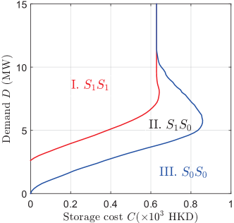
Figure 3: Equilibrium split with storage cost and demand at $\lambda=1.5$ HKD/kWh.

VI-B Impact of storage cost and demand on storage-investment equilibrium

We analyze the impact of storage cost and demand on the storage-investment equilibrium and have the analytical results for the cases when: (i) the storage cost $C_{i}$ is sufficiently large; (ii) the demand $D^{m,t}$ is sufficiently large or small. We present all the proofs in Appendix.XVII.

To better illustrate the storage-investment equilibrium, we show one simulation result of the equilibrium split (i.e., the storage-investment equilibrium with respect to parameters such as the demand and the storage cost) in Figure 3, and the details of the simulation setup are presented in Section VIII. In this simulation, for the illustration purpose, we consider the same demand $D$ for any hour $t$ of any month $m$. We also consider two homogeneous suppliers (with the same storage cost, the same renewable energy capacity and the same renewable energy distribution) to reveal the impact on storage-investment decision. In Figure 3 (where the penalty price is $\lambda=1.5$ Hong Kong dollars (HKD) per kWh), with respect to the demand and storage cost, the storage-investment equilibrium is divided into three regions: Region I of $\text{S}_{1}\text{S}_{1}$ (the left side of the red curve), Region II of $\text{S}_{1}\text{S}_{0}$ (between the red curve and the blue curve), and Region III of $\text{S}_{0}\text{S}_{0}$ (the right side of the blue curve).

First, for the impact of the storage cost, a higher storage cost will discourage suppliers from investing in storage as implied in Theorem 4. We will further show that when the storage cost is higher than a threshold, no suppliers will invest in storage no matter what the demand or penalty. However, counter-intuitively, we also find that in the case of a zero storage cost, not both suppliers will invest in storage once the demand is lower than a certain threshold.

As shown in Figure 3, when the storage cost is larger than a threshold, i.e., $C>0.86\times 10^{3}$ HKD, the $\text{S}_{0}\text{S}_{0}$ case will be the only equilibrium (independent of the demand $D$) and no suppliers invest in storage. We show this property in Proposition 6. The reason is that the benefit from investing in storage is bounded. When the storage cost is greater than a threshold corresponding to the bounded benefit, no suppliers will choose to invest in storage.

Proposition 6.

There exists a threshold $C_{i}^{\text{S}_{0}\text{S}_{0}}$ such that if the storage cost satisfies $C_{i}>C_{i}^{\text{S}_{0}\text{S}_{0}}$ for both $i=1,2$, the $\text{S}_{0}\text{S}_{0}$ case will be the unique pure storage-investment equilibrium.

However, as shown in Figure 3, when the demand is smaller than a certain threshold, i.e., $D<2.8$ MW, the $\text{S}_{1}\text{S}_{1}$ case cannot be a pure equilibrium even when the storage cost $C=0$. We show this property in Proposition 7. The reason is that when the demand is smaller than a certain threshold, in the $\text{S}_{1}\text{S}_{1}$ case, both suppliers can only get zero revenues (as shown in Proposition 2) due to the competition. Thus, if the $\text{S}_{1}\text{S}_{1}$ case is the storage-investment state where both suppliers invest in storage, one supplier can always deviate to not investing in storage, which can bring him a strictly positive profit as implied in Proposition 5.

Proposition 7.

If the demand satisfies $0<D^{m,t}\leq\min_{i}\mathbb{E}[X_{i}^{m,t}]$ for any $t$ and $m$, the $\text{S}_{1}\text{S}_{1}$ case cannot be the equilibrium.

Second, for the impact of demand, we already show that at a sufficiently low demand, the $\text{S}_{1}\text{S}_{1}$ case cannot be the equilibrium in Proposition 7. We will further show that if the demand is higher than a certain threshold, each supplier has a dominant strategy of whether to invest in storage based on his storage cost, which does not depend on the other supplier’s decision. For example, at $D>11$ MW in Figure 3, for these two homogeneous suppliers, if the storage cost is higher than a threshold, i.e., $C>0.63\times 10^{3}$ HKD, each supplier will not invest in storage (i.e., $\text{S}_{0}\text{S}_{0}$); otherwise, each supplier will invest (i.e., $\text{S}_{1}\text{S}_{1}$). We show this property in Proposition 8. The reason is that if the demand is large enough, both suppliers can bid the highest price and sell out the maximum bidding quantity. Thus, there is no competition between suppliers, and they will make storage-investment decisions based on their own storage costs.

Proposition 8.

There exists $D^{m,t,th}>0$ and $C_{i}^{\text{th}}>0$, such that when the demand satisfies $D^{m,t}\geq D^{m,t,th}$ for any $t$ and $m$, supplier $i$ has the dominant strategy $\varphi_{i}^{*}$ as follows.

$$\varphi_{i}^{*}=\left\{\begin{aligned} &1,~{}\text{if}~{}\text{the~{}storage~{}cost}~{}C_{i}\leq C_{i}^{\text{th}},\\ &0,~{}\text{if}~{}\text{the~{}storage~{}cost}~{}C_{i}>C_{i}^{\text{th}}.\end{aligned}\right.$$ (15)

VI-C Strictly positive profits of suppliers

We show that in suppliers’ competition facing the cost of storage investment, both suppliers can get strictly positive profits.

Proposition 9 (strictly positive profit).

Both suppliers will get strictly positive profits at the storage-investment equilibrium.

This proposition also shows the benefit of the uncertainty of renewable generation, which is similar to Proposition 5. Recall that if both suppliers have stable outputs, they may get zero revenue (shown in Proposition 2) and thus get negative profit considering the storage cost. However, with the random generation, both suppliers will get strictly positive profits at the storage-investment equilibrium even facing the storage cost. We will explain it as follows. Note that in the $\text{S}_{0}\text{S}_{0}$ case or the $\text{S}_{1}\text{S}_{0}$ case, the without-storage supplier always gets a strictly positive revenue (shown in Proposition 5) with a zero storage cost. In the $\text{S}_{1}\text{S}_{0}$ case or the $\text{S}_{1}\text{S}_{1}$ case, if the with-storage supplier gets a non-positive profit, he can always deviate to not investing in storage. This deviation provides him a strictly positive profit, which implies that the supplier will always get strictly positive profit.

VII Characterization of storage capacity

We propose a probability-based method using historical data of renewable generations to compute the storage capacity. Note that suppliers charge and discharge the storage to maintain his output at the mean value of the random renewable generations as shown in (1). Therefore, the charge and discharge amounts are also random variables, and we characterize the storage capacity such that its energy level will not exceed the storage capacity with a targeted probability. In this part, we focus on the storage with 100% charge and discharge efficiency and no degradation cost. In Appendix.XIII, we show that a lower charge/discharge efficiency and the consideration of degradation cost will increase the total storage cost of a supplier, which further affects the storage-investment equilibrium.

To begin with, we set a probability target $\alpha$, and we aim to find a storage capacity $S_{i}$ such that the energy level in the storage exceeds the capacity with a probability no greater than $\alpha$. Specifically, the with-storage supplier $i$ will charge and discharge storage with value $CD_{i}^{m,t}$ at hour $t$ of month $m$ as shown in (1). We assume that the initial energy level of storage is fixed for all the months and denote it as $S^{l}_{i}$. Note that the energy level of storage is the sum of the charge and discharge over the time, and is constrained by the storage capacity. Starting from the initial energy level $S^{l}_{i}$, the probability that energy level exceeds the minimum capacity (i.e., zero) and the maximum capacity (i.e., $S_{i}$) of the storage in a day of month $m$ is $\max_{t^{\prime}\in\mathcal{T}}\text{Pr}(\sum_{t=1}^{t^{\prime}}CD_{i}^{m,t}+S^{l}_{i}<0)$ and $\max_{t^{\prime}\in\mathcal{T}}\text{Pr}(\sum_{t=1}^{t^{\prime}}CD_{i}^{m,t}+S^{l}_{i}>S_{i})$, respectively. Considering all months $m$, we aim to choose the storage capacity $S_{i}$ so that the following hold:

$$\mathbb{E}_{m}\big{[}\max_{t^{\prime}\in\mathcal{T}}\text{Pr}(\sum_{t=1}^{t^{\prime}}CD_{i}^{m,t}+S^{l}_{i}<0)\big{]}\leq\alpha,$$ (16)

$$\mathbb{E}_{m}\big{[}\max_{t^{\prime}\in\mathcal{T}}\text{Pr}(\sum_{t=1}^{t^{\prime}}CD_{i}^{m,t}+S^{l}_{i}>S_{i})\big{]}\leq\alpha.$$ (17)

Then, we describe how to use historical data [29] to compute the storage capacity that satisfies the probability threshold as in (16) and (17). we will first characterize an upper bound for the probability that energy level exceeds the given storage capacity in terms of the random variable $CD_{i}^{m,t}$, and then we propose Algorithm 1 to compute the required storage capacity to satisfy (16) and (17).

First, given the underflow capacity $S_{i}^{l}>0$ and overflow capacity $S_{i}^{u}\triangleq S_{i}-S_{i}^{l}>0$, we characterize an upper bound $Pr^{l,m}(S_{i}^{l})$ for $\max_{t^{\prime}}\text{Pr}(\sum_{t=1}^{t^{\prime}}CD_{i}^{m,t}+S_{i}^{l}<0)$ and an upper bound $Pr^{u,m}(S_{i}^{u})$ for $\max_{t^{\prime}}\text{Pr}(\sum_{t=1}^{t^{\prime}}CD_{i}^{m,t}+S_{i}^{l}>S_{i})$, respectively. We characterize these upper bounds based on Markov inequality [30], which is shown in Proposition 10.

Proposition 10 (Markov-inequality-based upper bound).

Given $S_{i}^{l}>0$ and $S_{i}^{u}>0$, the Markov-inequality-based upper bounds are shown as follows.

• For the upper bound $Pr^{l,m}(S_{i}^{l})$:

  $$Pr^{l,m}(S_{i}^{l})=\max_{t^{\prime}}\min_{s>0}B^{l}(s),$$ (18)

  where $B^{l}(s)\triangleq e^{-sS_{i}^{l}}\cdot\mathbb{E}\left[e^{s\sum_{t=1}^{t^{\prime}}-CD_{i}^{m,t}}\right]$.

• For the upper bound $Pr^{u,m}(S_{i}^{u})$:

  $$Pr^{u,m}(S_{i}^{u})\triangleq~{}\max_{t^{\prime}}\min_{s>0}B^{u}(s),$$ (19)

  where $B^{u}(s)\triangleq e^{-sS_{i}^{u}}\cdot\mathbb{E}\left[e^{s\sum_{t=1}^{t^{\prime}}CD_{i}^{m,t}}\right]$.

Note that $Pr^{l,m}(S_{i}^{l})$ and $Pr^{u,m}(S_{i}^{u})$ are decreasing in $S_{i}^{l}$ and $S_{i}^{u}$, respectively. Also, $Pr^{l,m}(S_{i}^{l})\rightarrow 0$ as $S_{i}^{l}\rightarrow+\infty$, and $Pr^{u,m}(S_{i}^{u})\rightarrow 0$ as $S_{i}^{u}\rightarrow+\infty$. These show that a larger capacity will decrease the probability that the charge/discharge exceeds the capacity. Also, for any probability threshold $\alpha>0$, we can always find a capacity, such that the probability that energy level exceeds the capacity is below $\alpha$.

Second, we propose Algorithm 1 to characterize the storage capacity $S_{i}$ based on the historical data of $CD_{i}^{m,t}$ (derived from the renewable generation data of $X_{i}^{m,t}$). We use the underflow capacity $S_{i}^{l}$ for supplier $i$ as an example for illustration, and the overflow capacity $S_{i}^{u}$ follows the same procedure. Specifically, for the underflow capacity $S_{i}^{l}$, we search it in an increasing order from zero as in Step 4. Given $S_{i}^{l}$, for each month $m$, we calculate the exceeding probability $Pr^{l,m}(S_{i}^{l})$ according to (18) as in Steps 5-7. Note that based on the data samples of $\sum_{t=1}^{t^{\prime}}-CD_{i}^{m,t}$, $B^{l}(s)$ is strictly convex in $s$. Thus, for any $S_{i}^{l}>0$, the value of $\min_{s>0}B^{l}(s)$ can be efficiently computed using Newton’s method[31]. Further, we conduct an exhaustive search for ${t^{\prime}\in\mathcal{T}}$ to obtain $Pr^{l,m}(S_{i}^{l})$. We calculate the expected exceeding probability $\mathbb{E}_{m}[Pr^{l,m}(S_{i}^{l})]$ over months as in Step 8. We obtain the minimal underflow capacity $S_{i}^{l}$ if the exceeding probability satisfies $\mathbb{E}_{m}[Pr^{l,m}(S_{i}^{l})]\leq\alpha$ as in Step 9. Similarly, we can get the minimal overflow capacity $S_{i}^{u}$. The required storage capacity is calculated as in Step 11.

Algorithm 1 Storage capacity $S_{i}$

1:  initialization: set iteration index $S_{i}^{l}=S_{i}^{u}=0$, step size $\Delta S$;

2:  for each $k\in\{l,u\}$ do

3:     repeat

4:        $S_{i}^{k}:=S_{i}^{k}+\Delta S;$

5:        for each $m\in\mathcal{M}$ do

6:           Supplier $i$ calculates $Pr^{k,m}(S_{i}^{k})$ according to (18) or (19);

7:        end for

8:        Supplier $i$ calculates $\mathbb{E}_{m}[Pr^{k,m}(S_{i}^{k})]$;

9:     until 

$$\mathbb{E}_{m}[Pr^{k,m}(S_{i}^{k})]\leq\alpha;$$

10:  end for

11:  Each supplier $i$ computes

$$S_{i}=S_{i}^{l}+S_{i}^{u};$$

12:  output: $S_{i}$.

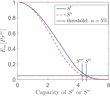
Figure 4: Characterization of storage capacity.

As an illustration, we calculate and show the underflow probability $\mathbb{E}_{m}[Pr^{l,m}(S_{i}^{l})]$ and overflow probability $\mathbb{E}_{m}[Pr^{u,m}(S_{i}^{u})]$ in the blue solid curve and red dashed curve respectively in Figure 4. The probability of $\mathbb{E}_{m}[Pr^{l,m}(S_{i}^{l})]$ ($\mathbb{E}_{m}[Pr^{u,m}(S_{i}^{u})]$, respectively) decreases with respect to the capacity $S_{i}^{l}$ ($S_{i}^{u}$, respectively). If the capacity $S_{i}^{l}$ ($S_{i}^{u}$, respectively) is small and close to zero, the exceeding probability $\mathbb{E}_{m}[Pr^{l,m}(S_{i}^{l})]$ ($\mathbb{E}_{m}[Pr^{u,m}(S_{i}^{u})]$, respectively) will approach one. However, when the capacity is large and close to a certain value (e.g., 6 in Figure 4), the corresponding exceeding probability will be close to zero. We choose the probability threshold $\alpha=5\%$ and obtain the corresponding minimal capacity $S_{i}^{l*}$ and $S_{i}^{u*}$ as marked in Figure 4.

VIII Simulation

In simulations, in addition to some analytical properties of storage-investment equilibrium shown in Section VI, we will further investigate the impact of the penalty, storage cost, and demand on suppliers’ profits. We will show some counter-intuitive results due to the competition between suppliers. For example, a higher penalty, a higher storage cost, and a lower demand can even increase a supplier’s profit at the storage-investment equilibrium. Furthermore, the first supplier who invests in storage may benefit less than the competitor who does not invest in storage. We will illustrate the detailed results in the following.

VIII-A Simulation setup

In simulations, we consider two homogeneous suppliers (with the same renewable capacity, generation distribution, and storage cost) to show the storage-investment equilibrium. We also consider a fixed demand $D$ for all the hours and months for illustration. Next, we explain the empirical distribution of renewable generation as well as parameter configurations of the penalty price $\lambda$, demand $D$, and storage cost $C$.

VIII-A1 Empirical distribution of renewable generation

We use the historical data of solar energy generation in Hong Kong from the year 1993 to year 2012 [29] to approximate the continuous CDF of suppliers’ renewable generations. Specifically, we cluster the renewable generations at hour $t$ of all days into $M=12$ types (months) considering the seasonal effect. We use daily data (from the year 1993 to year 2012) of renewable energy in month $m$ at hour $t$ to approximate the distribution of renewable generation at hour $t$ of month $m$. Based on the discrete data, we characterize a continuous empirical CDF to model the distribution of renewable power. We present the details of the characterization of empirical CDF in Appendix.XIV.

Furthermore, to check the reliability of the empirical distribution, we consider two sample data sets: one set consists of all the data samples from the year 1993 to 2012, and the other consists of the data samples from another specific year (e.g., 2013). We conduct Kolmogorov-Smirnov test [32] using the Matlab function kstest2 to test whether these two data sets are from the same continuous distribution [33]. The result shows that most of the hours of a month can pass the test. Also, our model is general for any continuous distribution of renewable generations. Interested readers can also use other data or other distributions of renewable energy to test the results.

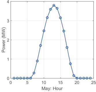
Figure 5: Average solar energy of different hours in May.

VIII-A2 Parameters configuration

We explain the configuration of the parameters of the penalty price $\lambda$, demand $D$, and storage cost $C$, respectively. We set the parameters to reflect the real-world practice, and study the impact of the parameters on the market equilibrium.

• The penalty $\lambda$: We choose the price cap $\bar{p}=1$ HKD/kWh, since the electricity price for residential users in Hong Kong is around 1 HKD/kWh [34]. Note that a penalty price satisfies $\lambda>\bar{p}$. In Figure 6(a), we will consider a wide range of the ratio $\frac{\lambda}{\bar{p}}\in[1.2,20]$ to demonstrate the impact of the penalty. In Figures 6(b)(c)(d), we fix the penalty price $\lambda=1.5$ HKD/kWh and focus on illustrating the impact of other parameters.

• The demand $D$: In Figure 6(d), we will discuss a wide range of demand from 0 MW to 15MW to show the impact of the demand. As a comparison, in Figure 5, we show the average renewable power across hours in May. In Figure 6(a) and (b), we fix the demand at $D=1$ MW to show the impact of other parameters ($\lambda$ and $C$). In Figure 6(c), we choose a larger demand $D=12$ MW and a smaller demand $D=6$ MW to show the impact of demand on the equilibrium profit.

• The Storage cost $C_{i}$: Recall that the storage investment cost is $C_{i}=c_{i}\kappa_{i}S_{i}$. There are different types of storage technologies with diverse capital costs and lifespans. For example, the pumped hydroelectric storage is usually cheap, and can last for 30 years with the capital cost $c_{i}=40\sim 800$ HKD/kWh, while the Li-ion battery can last 15 years with the capital cost about $c_{i}=1600\sim 9000$ HKD/kWh [35]. We choose the annual interest rate $r_{i}=5\%$, and the storage capacity for the with-storage supplier is characterized as 43 MWh by Algorithm 1. We capture the impact of parameters $c_{i}$ and $\kappa_{i}$ through the storage cost $C_{i}$. According to the calculation of storage investment cost $C_{i}=c_{i}\kappa_{i}S_{i}$, we can calculate that the (hourly) investment cost $C_{i}$ of the pumped hydroelectric storage is $0.012\times 10^{3}-0.255\times 10^{3}$ HKD and the cost of the Li-ion battery is $0.76\times 10^{3}-4.36\times 10^{3}$ HKD. This shows that the storage cost can have a wide range. Then, in Figures 6(c), we will consider a wide range of storage costs from 0 to $2\times 10^{3}$ HKD. Although zero storage cost is not very practical, we use it to show a low storage cost and capture the entire range of the impact of the storage costs. In Figure 6(a)(b)(d), we choose lower storage costs ($0.1\times 10^{3}$ and $0.15\times 10^{3}$ HKD) and higher storage costs ($1\times 10^{3}$ and $1.5\times 10^{3}$ HKD) to show the different results under different storage costs.

VIII-B Simulation results

We will discuss the impact of penalty, storage cost, and demand on suppliers’ profits, and show some counter-intuitive results due to the competition between suppliers.

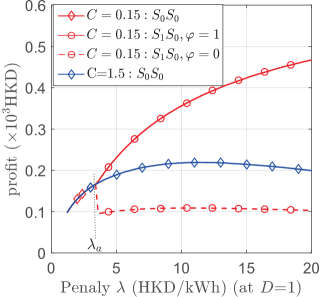
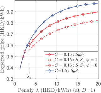
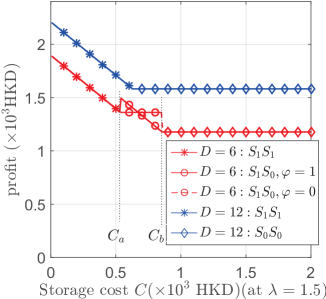
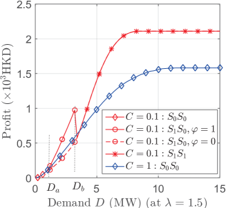
Figure 6: (a) Profit of suppliers with penalty ($D=1$ MW); (b) Expected bidding price of suppliers with penalty ($D=1$ MW); (c) Profit of suppliers with storage cost ($\lambda=1.5$ HKD/kWh); (d) Profit of suppliers with demand ($\lambda=1.5$ HKD/kWh).

VIII-B1 The impact of penalty on suppliers’ profits

Although a higher penalty $\lambda$ can increase the penalty cost on the without-storage supplier, surprisingly, we find that a higher penalty can also increase this supplier’s profit, due to the reduced market competition in the energy market.

We show how suppliers’ profits and expected bidding prices at the storage-investment equilibrium change with the penalty (at demand $D=1$ MW) in Figure 6 and 6, respectively. Different colors represent different storage costs. The diamond marker shows that $\text{S}_{0}\text{S}_{0}$ is the storage-investment equilibrium, and the circle marker shows that $\text{S}_{1}\text{S}_{0}$ is the equilibrium. Also, when $\text{S}_{1}\text{S}_{0}$ is the equilibrium, the solid lines and dashed lines distinguish the with-storage supplier and without-storage supplier, respectively.

First, we show that at the equilibrium where both suppliers do not invest in storage (i.e., $\text{S}_{0}\text{S}_{0}$), a higher penalty $\lambda$ can increase both suppliers’ profits. As shown in Figure 6, when the storage cost is high at $C=1.5\times 10^{3}$ HKD, both suppliers will not invest in storage for any value of the penalty $\lambda$ from $1.2$ HKD/kWh to $20$ HKD/kWh (in blue curve with diamond marker). In this case, both suppliers’ profits can first increase (at $\lambda<11$ HKD/kWh) and then decrease (at $\lambda>11$ HKD/kWh) with $\lambda$ (in blue curve). The intuition for the increase of profit at $\lambda<11$ HKD/kWh is that a higher penalty decreases both suppliers’ bidding quantity if the bidding price remains the same. This reduces the market competition and enables both suppliers to bid a higher price in the local energy market as shown in Figure 6 (in blue curve). However, the increased penalty also increases the penalty cost on suppliers, so the suppliers’ profits will also decrease if the penalty is too high (at $\lambda>11$ HKD/kWh).

Second, we show that at the equilibrium where one supplier invests in storage and one does not (i.e., $\text{S}_{1}\text{S}_{0}$), a higher penalty $\lambda$ can also increase both suppliers’ profits. We consider a low storage cost $C=0.15\times 10^{3}$ HKD as in red curves in Figure 6 and Figure 6. We see that if $\lambda$ is low (at $\lambda<\lambda_{a}$), both suppliers will not invest in storage (i.e., $\text{S}_{0}\text{S}_{0}$), and their profits increase with penalty shown in Figure 6 (at $\lambda<\lambda_{a}$ in red curve with diamond marker that overlaps with blue curve). As the penalty increases (at $\lambda>\lambda_{a}$), the equilibrium will change from $\text{S}_{0}\text{S}_{0}$ to $\text{S}_{1}\text{S}_{0}$, since a higher penalty and a lower storage cost can enable a supplier to enjoy more benefits by investing in storage. We discuss the profit of the with-storage supplier and without-storage supplier respectively as follows.

• For the with-storage supplier, as shown in Figure 6, when $\lambda>\lambda_{a}$, his profit increases as penalty increases (in red solid curve), which can be much higher than the without-storage supplier (in red dashed curve). The reason is that in the $\text{S}_{1}\text{S}_{0}$ case, the penalty cost makes the with-storage supplier dominate over the without-storage one. The with-storage supplier can bid higher prices than the without-storage supplier as shown in Figure 6 (in red solid curve and red dashed curve), and he also does not need to pay the penalty cost.

• However, for the without-storage supplier, as shown in Figure 6, his profit also slightly increases as the penalty increases around $\lambda_{a}<\lambda<10$ HKD/kWh (in red dashed curve). The intuition is that a higher penalty gives the advantage to the with-storage supplier, which reduces the market competition and increases both suppliers’ bidding price as shown in Figure 6 (in red curves). Thus, it can also benefit the without-storage supplier. However, as shown in Figure 6, if the penalty further increases to $\lambda>10$ HKD/kWh (in red dashed curve), the without-storage supplier’s profit will also decrease due to the increased penalty cost.

VIII-B2 The impact of storage cost on suppliers’ profits

Intuitively, a higher storage cost will discourage a supplier from investing in storage, which generally decreases a supplier’s profit. However, we find that it may also increase a supplier’s profit if the other supplier changes his strategy due to the increased storage cost.

We show how suppliers’ profits at the storage-investment equilibrium change with the storage cost in Figure 6. Different colors represent different demands. The diamond marker, circle marker, and star marker correspond to different storage-investment equilibria of $\text{S}_{0}\text{S}_{0}$, $\text{S}_{1}\text{S}_{0}$, and $\text{S}_{1}\text{S}_{1}$, respectively. For the $\text{S}_{1}\text{S}_{0}$ case, the solid lines and dashed lines distinguish the with-storage supplier and without-storage supplier, respectively.

As shown in Figure 6 (in both red curve and blue curve), generally the higher storage cost decreases suppliers’ profits. However, we show that the opposite may be true using the example of $D=6$ MW (in red curve). When the demand is at $D=6$ MW (in red curve), as the storage cost increases, the equilibrium changes from $\text{S}_{1}\text{S}_{1}$ (when $C<C_{a}$), to $\text{S}_{1}\text{S}_{0}$ (when $C_{a}<C<C_{b}$), and finally to $\text{S}_{0}\text{S}_{0}$ (when $C>C_{b}$). When the equilibrium changes from $\text{S}_{1}\text{S}_{1}$ to $\text{S}_{1}\text{S}_{0}$ at the threshold $C=C_{a}$, one with-storage supplier in the original $\text{S}_{1}\text{S}_{1}$ case has a higher (upward jumping) profit, after the other supplier chooses not to invest in storage due to the high storage cost. This changes the equilibrium from $\text{S}_{1}\text{S}_{1}$ to $\text{S}_{1}\text{S}_{0}$, which reduces the competition and gives more advantages to the with-storage supplier.

VIII-B3 The impact of demand on suppliers’ profits

Intuitively, a higher demand will increase a supplier’s profit. However, we show that a higher demand may also decrease a supplier’s profit if the other supplier changes his strategy due to the increased demand.

We show how suppliers’ profits at the storage-investment equilibrium change with the demand in Figure 6. Different colors represent different storage costs. The diamond marker, circle marker, and star marker correspond to different storage-investment equilibria of $\text{S}_{0}\text{S}_{0}$, $\text{S}_{1}\text{S}_{0}$, and $\text{S}_{1}\text{S}_{1}$, respectively. For the $\text{S}_{1}\text{S}_{0}$ case, the solid lines and dashed lines distinguish the with-storage supplier and without-storage supplier respectively.

As shown in Figure 6 (in both red curve and blue curve), generally a higher demand increases a supplier’s profit. However, we show that the opposite may be true using the example of $C=0.1\times 10^{3}$ HKD (in red curve). When the storage cost is low at $C=0.1\times 10^{3}$ HKD (in red curve), as the demand increases, the equilibrium changes from $\text{S}_{0}\text{S}_{0}$ (when $D<D_{a}$), to $\text{S}_{1}\text{S}_{0}$ (when $D_{a}<D<D_{b}$), and finally to $\text{S}_{1}\text{S}_{1}$ (when $D>D_{b}$). When the equilibrium changes from $\text{S}_{1}\text{S}_{0}$ to $\text{S}_{1}\text{S}_{1}$ at the threshold $D=D_{b}$, the with-storage supplier in the original $\text{S}_{1}\text{S}_{0}$ case has a smaller (downward jumping) profit, after the other supplier also chooses to invest in storage due to the high demand. This changes the equilibrium from $\text{S}_{1}\text{S}_{0}$ to $\text{S}_{1}\text{S}_{1}$, which increases the market competition and weakens the advantage of the with-storage supplier in the original $\text{S}_{1}\text{S}_{0}$ case. Furthermore, when the storage cost is high at $C=1.5\times 10^{3}$ HKD (in blue curve with diamond marker), both suppliers will not invest in storage independent of the demand.

VIII-B4 First-mover disadvantage and advantage

Intuitively, the first supplier who invests in storage can benefit more than the without-storage competitor. However, we find that if the storage cost is high, the first-mover supplier in investing storage can also benefit less than the free-rider competitor who does not invest in storage.

As shown in Figure 6 at $D=6$ MW (in red curve), the $\text{S}_{1}\text{S}_{0}$ case is the equilibrium when the storage cost is in the range $C_{a}<C<C_{b}$. If the storage cost is low at $C_{a}<C<0.7\times 10^{3}\text{ HKD}$, the with-storage supplier’s profit is higher than the without-storage supplier’s profit. However, if the storage cost is high at $0.7\times 10^{3}\text{ HKD}<C<C_{b}$, the with-storage supplier’s profit is lower than the without-storage supplier. This shows both advantage and disadvantage of the first-mover. Although in some situations investing storage will increase the supplier’s profit, he can get more profits if he waits for the other to invest first when the storage cost is high. However, if the storage cost is low, he should be the first to invest storage in order to get a higher profit.

IX Extensions: A more general oligopoly model

We build a more general oligopoly model and extend some of the theoretical results and insights from the duopoly case to the oligopoly case. Compared with the duopoly model, the only difference of the oligopoly model is that the number of suppliers can be more than two, i.e., $|\mathcal{I}|\geq 2$. Following the analysis of the duopoly model, we also analyze the equilibrium in Stage II and Stage I in the oligopoly case and derive some insights. Specifically, in Stage II, we extend the theoretical results of the price-quantity competition equilibrium. In Stage I, we generalize analytical results of the impact of storage cost and demand on the storage-investment equilibrium. Furthermore, we show that some of the key insights from the duopoly case, e.g., the uncertainty of renewable generation can be beneficial to suppliers, still hold in the oligopoly case. Next, we will discuss the extensions of Stage II and Stage I in detail, respectively. We include all the proofs of the propositions in Appendix.XVIII.

IX-A Stage II Analysis

For Stage II, the weakly dominant strategy of bidding quantities still hold for the case of more than two suppliers. We generalize the conditions on the existence of the pure price equilibrium and show that the mixed price equilibrium also exists in the oligopoly case. Furthermore, we show that suppliers get positive revenues at the mixed price equilibrium. We show the extended analysis in detail as follows.

IX-A1 Weakly dominant strategy for bidding quantities

The weakly dominant strategies for bidding quantities still hold as in Theorem 1.

IX-A2 Existence of the pure price equilibrium

We derive the conditions for the existence of the pure price equilibrium among suppliers, and generalize Proposition 2. Specifically, we consider a general subgame in Stage II denoted as ${S}^{{\mathcal{U}|\mathcal{V}}}$, where suppliers in the set $\mathcal{U}$ invest in storage and suppliers in the set $\mathcal{V}$ do not invest. Recall we denote the set of all the suppliers as $\mathcal{I}$, and we have $\mathcal{U}\bigcup\mathcal{V}=\mathcal{I}$. The case $\mathcal{U}=\mathcal{I}$ means that all the suppliers invest in storage, and the case $\mathcal{V}=\mathcal{I}$ means that no supplier invests in storage. We show the existence of the pure price equilibrium in Proposition 11.

Proposition 11 (existence of the pure price equilibrium in the oligopoly case).

Considering a subgame $\text{S}^{{\mathcal{U}|\mathcal{V}}}$ of storage investment among suppliers in Stage II, the existence of the pure price equilibrium depends on the demand $D$ as follows:

• If $D\geq\sum_{i\in\mathcal{I}}y_{i}^{*}(\bar{p},\varphi_{i})$, there exists a pure price equilibrium $p_{i}^{*}=\bar{p}$, with an equilibrium revenue $\pi_{i}^{RE}=\lambda\int_{0}^{F_{i}^{-1}(\bar{p}/\lambda)}xf_{i}(x)dx$ for any $i\in\mathcal{V}$ and $\pi_{i}^{RE}=\bar{p}\mathbb{E}[X_{i}]$ for any $i\in\mathcal{U}$.

• If $D\leq\sum_{i\in\mathcal{U}}y_{i}^{*}(\bar{p},\varphi_{i})-y_{j}^{*}(\bar{p},\varphi_{j})$ for any $j\in\mathcal{U}$, there exists a pure price equilibrium $p_{i}^{*}=0$, with an equilibrium revenue $\pi_{i}^{RE}=0$, for any $i\in\mathcal{I}$.

• If there exists $j\in\mathcal{U}$ such that $\sum_{i\in\mathcal{U}}y_{i}^{*}(\bar{p},\varphi_{i})-y_{j}^{*}(\bar{p},\varphi_{j})<D<\sum_{i\in\mathcal{I}}y_{i}^{*}(\bar{p},\varphi_{i})$, there is no pure price equilibrium.

Similar to the duopoly case, the result of this proposition can be interpreted as follows. If the demand is higher than the threshold $\sum_{i\in\mathcal{I}}y_{i}^{*}(\bar{p},\varphi_{i})$, all the suppliers can bid the price cap to sell the maximum quantities. If the demand is very low such that $D\leq\sum_{i\in\mathcal{U}}y_{i}^{*}(\bar{p},\varphi_{i})-y_{j}^{*}(\bar{p},\varphi_{j})$ for any $j\in\mathcal{U}$, the competition is fierce and all the suppliers bid zero price. However, if the demand is in the middle, there will be no pure price equilibrium.

Note that if the number of with-storage suppliers is no greater than one, i.e., $\mid\mathcal{U}\mid\leq 1$, the condition that there exists $j\in\mathcal{U}$ such that $D\leq\sum_{i\in\mathcal{U}}y_{i}^{*}(\bar{p},\varphi_{i})-y_{j}^{*}(\bar{p},\varphi_{j})$ cannot be satisfied. It means that there will be no pure equilibrium of $p_{i}^{*}=0$ for any demand $D>0$.

IX-A3 Existence of the mixed price equilibrium

For the case in Proposition 11 that there exists no pure price equilibrium, we show that there exists a mixed price equilibrium. However, the characterization of mixed strategy is highly non-trivial for the oligopoly case and it is difficult to completely generalize Lemma 1. We generalize it partially as Proposition 12 to show the existence of the mixed price equilibrium and show that all the suppliers get positive revenues at the mixed price equilibrium.

Proposition 12 (mixed price equilibrium in the oligopoly case).

For any $\bm{\varphi}$, when there is no pure price equilibrium, a mixed price equilibrium exists and the equilibrium electricity-selling revenues $\pi_{i}^{RE}$ satisfies $\pi_{i}^{RE}(\bm{\varphi})>0,\text{~{}for any}~{}i\in\mathcal{I}$.

The equilibrium revenue for the case where all the suppliers invest storage (i.e., $\mathcal{U}=\mathcal{I}$) has been characterized in [17]. When there are two suppliers, we can also characterize the cumulative distribution function (CDF) of the mixed price strategy for the case of one investing storage and one not investing in storage as in Theorem 2. However, when $I>2$, for any case where $\mid\mathcal{U}\mid<I$, it is highly non-trivial to characterize the corresponding CDF analytically.

IX-B Stage I Analysis

For Stage I, for the general oligopoly case, we show that a mixed storage-investment equilibrium always exists. We can also generalize the analytical results of the impact of storage cost and demand on the storage-investment equilibrium for those settings where (i) the storage cost is sufficiently large; and (ii) the demand is sufficiently large or small. Furthermore, some of the key insights, e.g., the uncertainty of renewable generation can be beneficial to suppliers, will still hold for the oligopoly case. We discuss the extensions in details in the following.

IX-B1 Existence of the storage-investment equilibrium

A mixed equilibrium of storage investment always exists. Note that each supplier has two strategies: investing in storage and not investing in storage. Numerically, we can check the pure storage-investment equilibrium by the Nash equilibrium definition. Also, a mixed equilibrium of storage investment always exists due to the finite numbers of storage-investment strategies [28].

IX-B2 Impacts of the storage cost and demand on storage-investment equilibrium

Some analysis of the impact of the storage cost and demand on storage-investment equilibrium in the duopoly case can also be extended. Specifically, we can extend Propositions 6, 7 and 8 and to the oligopoly case, which generalizes the analytical results for the settings where (i) the storage cost is sufficiently large; and (ii) the demand is sufficiently large or small.

First, since the benefit from investing in storage is bounded, we can show that when the storage cost is greater than a threshold, no suppliers will choose to invest in storage.

Proposition 13.

There exists a threshold $C_{i}^{\text{no}}$ such that if the storage cost satisfies $C_{i}>C_{i}^{\text{no}}$ for any $i\in\mathcal{I}$, the $S^{\emptyset|\mathcal{I}}$ case (i.e., no suppliers investing in storage) will be the unique pure storage-investment equilibrium.

Second, in the subgame $S^{\mathcal{U}|\mathcal{V}}$ where $\mid\mathcal{U}\mid\geq 2$, if the demand is too low, all the suppliers may get zero revenue in the energy market as implied in Proposition 11. This will make the with-storage suppliers deviate to not investing in storage. Thus, we have the proposition as follows.

Proposition 14.

In the subgame $S^{\mathcal{U}|\mathcal{V}}$, if the demand satisfies $0<D^{m,t}\leq\min_{j\in\mathcal{U}}(\sum_{i\in\mathcal{U}}y_{i}^{*}(\bar{p},\varphi_{i})-y_{j}^{*}(\bar{p},\varphi_{j}))$ for any $t$ and $m$, the case $S^{\mathcal{U}|\mathcal{V}}$ (i.e., suppliers in set $\mathcal{U}$ invest in storage and suppliers in set $\mathcal{V}$ do not invest in storage) cannot be a pure storage-investment equilibrium.

Third, as in Proposition 11, when the demand is higher than certain threshold, all the suppliers can bid the price cap to sell all his bidding quantity. In this case, there is no competition between suppliers, and they will make storage-investment decisions independently based on their own storage costs. We show this proposition as follows.

Proposition 15.

There exist $D^{m,t,th}>0$ and $C_{i}^{\text{th}}>0$, such that when the demand satisfies $D^{m,t}\geq D^{m,t}_{\text{th}}$ for any $t$ and $m$, supplier $i$ has the dominant strategy $\varphi_{i}^{*}$ as follows.

$$\varphi_{i}^{*}=\left\{\begin{aligned} &1,~{}\text{if}~{}\text{the~{}storage~{}cost}~{}C_{i}\leq C_{i}^{\text{th}},\\ &0,~{}\text{if}~{}\text{the~{}storage~{}cost}~{}C_{i}>C_{i}^{\text{th}}.\end{aligned}\right.$$ (20)

IX-B3 Positive profits at the storage-investment equilibrium

We can further extend Proposition 9 to show the benefit of the uncertainty to the equilibrium profit. We show that in suppliers’ competition (even with the potential cost of the storage investment), all the suppliers can get strictly positive profits at the equilibrium.

Proposition 16 (strictly positive profit).

All the suppliers will get strictly positive profits at the storage-investment equilibrium.

This proposition shows the benefit of the renewable generation randomness. If all the suppliers have stable outputs, they may get zero revenue as implied in Proposition 11 and thus get negative profit under possible storage cost. However, with the random generation, all the suppliers will get strictly positive profit at the storage-investment equilibrium even considering the storage cost. The intuition is that if one supplier invests in storage and gets non-positive profit, he can always choose not to invest in storage. This at least saves him the cost of storage investment, which increases his profit. Also, note that when no supplier invests in storage, all the suppliers can get positive profits. Therefore, only the state where all the suppliers get positive profits can be an equilibrium.

In summary, we can extend some of our major theoretical results and insights to the oligopoly case of more than two suppliers. Some of the key insights from the duopoly case, e.g., the uncertainty of renewable generation can be beneficial to suppliers, still hold in the oligopoly case. However, we are not able to analytically extend all insights to the oligopoly case due to the complexity of analysis. We would like to explore it in our future work.

X Conclusion

We study a duopoly two-settlement local energy market where renewable energy suppliers compete to sell electricity to consumers with or without energy storage. We formulate the interactions between suppliers and consumers as a three-stage game-theoretic model. We characterize a price-quantity competition equilibrium in the local energy market, and further characterize a storage-investment equilibrium at the beginning of the investment horizon between suppliers. Surprisingly, we find the uncertainty of renewable generation can increase suppliers’ profits compared with the case where both suppliers invest in storage and stabilize the outputs. In simulations, we show more counterintuitive results due to the market competition. For example, a higher penalty, a higher storage cost, and a lower demand may increase a supplier’s profit. We also show that the first-mover in investing in storage may benefit less than the free-rider competitor who does not invest in storage. In the future work, we will size the variable storage capacity considering the possibility of not completely smoothing out the renewable output.

Appendix

This appendix is organized as follows:

• Section XI: We show the equilibrium revenue of suppliers in the $\text{S}_{1}\text{S}_{1}$ case, when the demand satisfies $\min_{i}y_{i}^{*}(\bar{p},\varphi_{i})<D<\sum_{i}y_{i}^{*}(\bar{p},\varphi_{i})$ and there is no pure price equilibrium but the mixed price equilibrium.

• Section XII: We show how we discretize the continuous price set to approximate the mixed price equilibrium in the $\text{S}_{0}\text{S}_{0}$ case.

• Section XIII: For the storage capacity characterization, we first show the proof of the propositions in Section VII, and then we present the model of the imperfect storage.

• Section XIV: For the simulations, we first show the characterization of the continuous CDF for the renewable-generation distribution using historical data, and then we simulate an example of two heterogeneous suppliers.

• Section XV: We prove the theorems and propositions of Stage III.

• Section XVI: We prove the theorems and propositions of Stage II.

• Section XVII: We prove the theorems and propositions of Stage I.

• Section XVIII: We prove the propositions in the oligopoly model.

XI Appendix: Mixed price equilibrium of $\text{S}_{1}\text{S}_{1}$ subgame

As shown in Proposition 2, when the demand satisfies $\min_{i}y_{i}^{*}(\bar{p},\varphi_{i})<D<\sum_{i}y_{i}^{*}(\bar{p},\varphi_{i})$, there is no pure price equilibrium. We can characterize a close-form equilibrium revenue for each supplier at the mixed price equilibrium in Proposition 17, which has been proved in [17].

Proposition 17 ($\text{S}_{1}\text{S}_{1}$: mixed-equilibrium revenue).

In the $\text{S}_{1}\text{S}_{1}$ case (i.e., $\sum_{i=1}\varphi_{i}=2$), if $\min_{i}y_{i}^{*}<D<\sum_{i}y_{i}^{*}$, there exists no pure price equilibrium but exists the mixed price equilibrium, with the equilibrium revenue as follows.

$$\pi_{i}^{RE}(\bm{\varphi})=\left\{\begin{aligned} &\bar{p}(D-y_{-i}^{*}),~{}{if}~{}y_{i}^{*}>y_{-i}^{*},\\ &\frac{\bar{p}(D-y_{i}^{*})y_{i}^{*}}{\min(y_{-i}^{*},D)},~{}otherwise,\\ \end{aligned}\right.$$

where $y_{i}^{*}=\mathbb{E}[X_{i}]$ and $y_{-i}^{*}=\mathbb{E}[X_{-i}]$ as characterized in Theorem 1.

According to Proposition 17, one supplier’s equilibrium revenue is related to the other supplier’s bidding quantity (i.e., mean value of generations). Specifically, one supplier’s equilibrium revenue decreases if the other supplier’s bidding quantity increases. Furthermore, under the mixed price equilibrium, both suppliers get strictly positive revenues while they may get zero revenues when the demand is below the threshold $\min_{i}y_{i}^{*}$ as shown in Proposition 2 under the pure price equilibrium.

XII Appendix: Mixed price equilibrium of $\text{S}_{0}\text{S}_{0}$ subgame

In the $\text{S}_{0}\text{S}_{0}$ case, both suppliers do not invest in storage and face the general penalty cost. When $0<D<\sum_{i}y_{i}^{*}(\bar{p},\varphi_{i})$, the mixed price equilibrium has a continuous CDF over $[l,\bar{p})$ shown in Lemma 1, but we cannot derive it in close form. To have a better understanding of the CDF, we discretize the price to approximate the original continuous price set, and compute the mixed equilibrium for the discrete price set.

Specifically, we discretize the price between $(0,\bar{p}]$ into $\{\Delta p,2\Delta p,3\Delta p,...,\bar{p}-\Delta p,\bar{p}\}$ with a small $\Delta p>0$. We search for the lower support in the range given in (14) in the following way. Given a lower support $l^{\prime}$, the mixed strategy of each supplier has the support $\{l^{\prime},l^{\prime}+\Delta p,l^{\prime}+\Delta p,...,\bar{p}\}$ that approximates the original continuous support $[l,\bar{p}]$. For each supplier, each of price strategies in the support yields the same expected revenue, which can be used to construct a set of linear equations and calculate the mixed equilibrium. If the probability of each price for each supplier is between $(0,1)$, then the lower support $l^{\prime}$ is feasible; otherwise, there exists the price that should be excluded from the support $\{l^{\prime},l^{\prime}+\Delta p,l^{\prime}+\Delta p,...,\bar{p}\}$ and the lower support $l^{\prime}$ is not feasible. We calculate the equilibrium revenue according to Lemma 1 (ii).

XIII Appendix: Characterization of storage capacity

We will first prove Proposition 10 and show some properties of the upper bound $Pr^{l,m}(S_{i}^{l})$ and $Pr^{u,m}(S_{i}^{u})$. Then, we discuss the imperfect storage model and show how it affects the storage cost.

XIII-A Proof of Proposition 10

Proof: Below, we illustrate the upper bound $Pr^{l,m}(S_{i}^{l})$. The upper bound $Pr^{u,m}(S_{i}^{u})$ can be derived analogously.

Given $t^{\prime}\in\mathcal{T}$, we have

$$\text{Pr}(\sum_{t=1}^{t^{\prime}}-CD_{i}^{m,t}>S_{i}^{l}) =\text{Pr}\left(e^{s\sum_{t=1}^{t^{\prime}}-CD_{i}^{m,t}\geq e^{sS_{i}^{l}}}\right)\leq e^{-sS_{i}^{l}}\cdot\mathbb{E}\left[e^{s\sum_{t=1}^{t^{\prime}}-CD_{i}^{m,t}}\right]\triangleq B^{l}(s),$$ (21)

for any $s>0$. The inequality in (21) is due to the Markov inequality. Given $S_{i}^{l}>0$, we can find a tight upper bound for the probability $\text{Pr}(\sum_{t=1}^{t^{\prime}}-CD_{i}^{m,t}>S_{i}^{l})$ by minimizing the RHS in (21) over $s$. Therefore, $Pr^{l,m}(S_{i}^{l})=\max_{t^{\prime}}\min_{s>0}B^{l}(s)$. ∎

XIII-B Properties of some properties of the upper bound $Pr^{l,m}(S_{i}^{l})$ and $Pr^{u,m}(S_{i}^{u})$.

We have properties for $Pr^{l,m}(S_{i}^{l})$ and $Pr^{u,m}(S_{i}^{u})$ as follows.

Proposition 18 (properties of the upper bounds).

Given $S_{i}^{l}>0$ and $S^{u}>0$, the Markov-inequality-based upper bounds have properties as follows.

1. $Pr^{l,m}(S_{i}^{l})\leq 1$ and $Pr^{u,m}(S_{i}^{u})\leq 1$.

2. $Pr^{l,m}(S_{i}^{l})$ and $Pr^{u,m}(S_{i}^{u})$ are decreasing in $S_{i}^{l}$ and $S_{i}^{u}$, respectively.

3. $Pr^{l,m}(S_{i}^{l})\rightarrow 0$ as $S_{i}^{l}\rightarrow+\infty$, and $Pr^{u,m}(S_{i}^{u})\rightarrow 0$ as $S_{i}^{u}\rightarrow+\infty$.

Proof: The first property is because $\min_{s>0}B^{l}(s)\leq B^{l}(0^{-})=1$ and $\min_{s>0}B^{u}(s)\leq B^{u}(0^{-})=1$. The second property is straightforward from the function $B^{l}(s)$ and $B^{u}(s)$. The third property is because $CD_{i}^{m,t}$ is bounded. Thus, $B^{l}(s)\rightarrow 0$ as $S_{i}^{l}\rightarrow+\infty$, and $B^{u}(s)\rightarrow 0$ as $S_{i}^{u}\rightarrow+\infty$. ∎

Proposition 18 shows that a larger capacity decreases the charge/discharge exceeding probability. Also, for any positive probability threshold $\alpha$, we can always find a sufficiently large capacity to let the exceeding probability below $\alpha$. This lays the foundation for Algorithm 1.

XIII-C Generalization of imperfect storage model

We consider the imperfect energy storage in two aspects: (i) less-than-100% charge and discharge efficiency and (ii) the degradation cost incurred by the charge and discharge. Next, we will explain how the storage charge and discharge are determined in our work, and then further discuss how the imperfect storage impacts the total storage cost and investment equilibrium.

To begin with, we explain the model of the storage charge and discharge as well as the energy level of the storage in our work. Specifically, the with-storage supplier charges and discharges the energy storage to stabilize his renewable output at the mean value. Thus, the charge and discharge power is only dependent on the random variable of renewable generations. At hour $t$ of renewable-generation-type (month) $m$, we denote the charge amount as $CD_{i}^{m,t+}\geq 0$ and the discharge amount as $CD_{i}^{m,t-}\geq 0$. These values are characterized based on the random generation $X_{i}^{m,t}$ as follows:

$$CD_{i}^{m,t+}=(X_{i}^{m,t}-\mathbb{E}[X_{i}^{m,t}])^{+},$$ (22)

$$CD_{i}^{m,t-}=(X_{i}^{m,t}-\mathbb{E}[X_{i}^{m,t}])^{-},$$ (23)

where $g^{+}\triangleq\max(g,0)$ and $g^{-}\triangleq\max(-g,0)$. Furthermore, we denote the charge efficiency as $\eta_{i}^{c}$ and the discharge efficiency as $\eta_{i}^{d}$. The energy level in the storage can be calculated by adding the charge and discharge over time at month $m$ as follows.

$$e_{i}^{m,t}=e_{i}^{m,t-1}+\eta_{i}^{c}CD_{i}^{m,t+}-CD_{i}^{m,t-}/\eta_{i}^{d}.$$ (24)

Next, we discuss how the degradation cost and the less-than-100% charge and discharge efficiency impact the total storage cost.

XIII-C1 Degradation cost

We show that the degradation cost will increase the total cost of deploying the storage for the with-storage supplier. The degradation cost is caused by the charge and discharge of the storage. In the ideal case, we do not include the degradation cost as part of the storage cost. With the degradation, the total cost of deploying the storage will be higher. One widely used model in the literature for the degradation cost is a linear model [37][38]. We denote the unit cost of charge and discharge as $c_{i}^{o}$. Thus, the expected degradation cost $C_{i}^{o}$ (in each hour) is

$$C_{i}^{o}=\mathbb{E}_{m,t}[c_{i}^{o}CD_{i}^{m,t+}+c_{i}^{o}CD_{i}^{m,t-}],$$ (25)

which can be calculated based on the historical data of $X_{i}^{m,t}$.

Therefore, We can simply add (25) to the original storage cost. We calculate the total storage cost as $C_{i}^{\prime}=C_{i}+C_{i}^{o}$, which includes both investment cost and the degradation cost.

XIII-C2 Charge and discharge efficiency

The lower charge and discharge efficiency will increase the storage capacity and thus increase the total storage cost. Our goal is to characterize a minimum storage capacity such that the energy level $e_{i}^{m,t}$ will exceed the storage capacity with a probability no greater than $\alpha$. As shown in (24), the charge and discharge efficiency ($\eta_{i}^{c},~{}\eta_{i}^{d}$) will affect the energy level $e_{i}^{m,t}$. Compared with the perfect storage model with $\eta_{i}^{c}=\eta_{i}^{d}=100\%$, the difference in the imperfect storage model is that $\eta_{i}^{c}<100\%$ and $\eta_{i}^{d}<100\%$. With the charge and discharge efficiency, we modify (16) and (17) in Section XIII.A into the following.

$$\mathbb{E}_{m}\big{[}\max_{t^{\prime}\in\mathcal{T}}\text{Pr}(\sum_{t=1}^{t^{\prime}}\eta_{i}^{c}CD_{i}^{m,t+}-CD_{i}^{m,t-}/\eta_{i}^{d}+S^{l}_{i}<0)\big{]}\leq\alpha,$$ (26)

$$\mathbb{E}_{m}\big{[}\max_{t^{\prime}\in\mathcal{T}}\text{Pr}(\sum_{t=1}^{t^{\prime}}\eta_{i}^{c}CD_{i}^{m,t+}-CD_{i}^{m,t-}/\eta_{i}^{d}+S^{l}_{i}>S_{i})\big{]}\leq\alpha.$$ (27)

Similarly, we can follow Algorithm 1 in Section XIII.A to compute $S_{i}$ given the probability threshold $\alpha$.

According to Algorithm 1 that computes the storage capacity, we show how charge/discharge efficiency impacts the storage capacity in Figure 7. The blue curve shows the case where the probability that the energy level exceeds the capacity is smaller than 5% and the red curve shows the case where the probability that the energy level exceeds the capacity is smaller than 10%. We see that as the efficiency decreases, the required storage capacity increases (which further increases the storage investment cost).

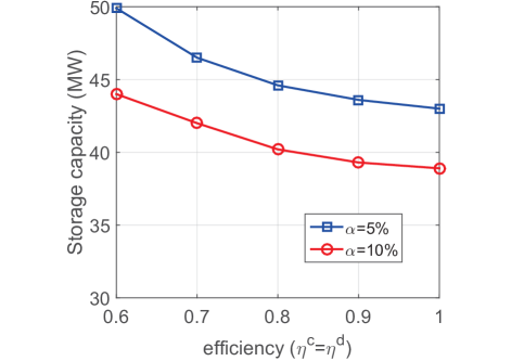
Figure 7: Storage capacity with charge/discharge efficiency.

In summary, compared with the case of perfect storage, a lower charge/discharge efficiency with the degradation cost will increase the total storage cost of a supplier. In Section VI, we present some analytical results of the storage cost’ s impact on the storage-investment equilibrium. In Section VIII, we also show the simulation results of the impact of the storage cost on the suppliers’ profits. These discussions can capture the impact of the imperfect storage.

XIV Appendix: Simulations

We will first show the details of how we approximate the continuous CDF for the renewable-generation distribution using historical data. Then, we show a simulation result for two heterogeneous suppliers.

XIV-A Empirical distribution of renewable generations

We use the historical data of solar energy in Hong Kong from the year 1993 to year 2012 [29] to approximate the continuous CDF of suppliers’ renewable generations. Specifically, we cluster the renewable generations at hour $t$ of all days into $M=12$ types (months) considering the seasonal effect. We use daily data (from the year 1993 to year 2012) of renewable energy in month $m$ at hour $t$ to approximate the distribution of renewable generation at hour $t$ of month $m$. Based on the discrete data, we first use an empirical cumulative distribution function (ECDF) to model the renewable power distribution. Note that our model is built on the continuous CDF of suppliers’ renewable generations. Thus, we further use linear interpolation to set up the continuous ECDF from the ECDF[40]. We illustrate the ECDF and linearly-interpolated ECDF in Figure 8, where the stepwise blue solid curve represents the ECDF and the red dotted curve represents the linearly-interpolated ECDF. For the illustration of renewable generation distribution, we show the ECDF and linearly-interpolated ECDF of hour $t=9$ of month $m=5$ (May) in Figure 8. Through the linearly-interpolated ECDF $F_{i}$, we can also compute the value $F_{i}^{-1}(\cdot)$ efficiently.

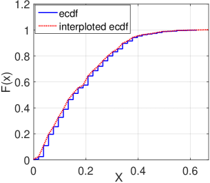
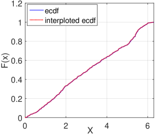
Figure 8: (a) Illustration of ECDF and linearly-interpolated ECDF; (b) ECDF and linearly-interpolated ECDF at hour 9 of May.

XIV-B Simulations of two heterogeneous suppliers

We simulate an example with two heterogeneous suppliers. Note that we can prove that a pure Nash equilibrium of storage investment will always exist in the homogeneous case (with the same storage cost, the same renewable energy capacity and the same renewable energy distribution). However, for the general heterogeneous case, we cannot theoretically prove that the pure Nash equilibrium always exists. In our following example of heterogeneous suppliers, the pure Nash equilibrium of storage investment still exists.

Specifically, we consider that supplier 2’s renewable generation capacity is twice as much as the capacity of supplier 1, where both suppliers have the same distribution of renewable energy. For comparison, we consider the homogeneous case as in the simulation of the main text where each supplier’s renewable generation capacity is equal to supplier 1’s capacity of the heterogeneous case. In the following, we first assume that the storage investment cost is the same across the two suppliers, and study the storage-investment equilibrium with respect to the storage cost and demand in the homogeneous (capacity) case and heterogeneous (capacity) case, respectively. Then, we allow the storage investment cost to also differ across the two suppliers in the heterogeneous case, and study the storage-investment equilibrium with respect to the two suppliers’ different storage costs.

We first consider the case that two suppliers’ bear the same investment cost of storage, so as to focus on showing the impact of different capacities of renewables. Figure 9 shows the equilibrium split in terms of demand and storage cost under the homogeneous case. Note that this figure has been shown as Figure 3 of the main text. Figure 9 shows the equilibrium split in terms of demand and storage cost under the heterogeneous case.

• In Figure 9, in Region I, both-investing-storage is one equilibrium; in Region III, neither-investing-storage is one equilibrium; in Region II, one investing in storage and one not investing in storage will be one equilibrium.

• In Figure 9, in the solid-grid region, both-investing-storage is one equilibrium; in the dash-grid region, neither-investing-storage is one equilibrium; in the region bounded by the red curve, supplier 1 does not invest in storage while supplier 2 should invest in storage; and in the region bounded by the blue curve, supplier 1 invests in storage while supplier 2 does not invest in storage.

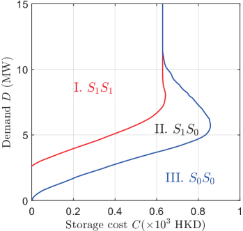
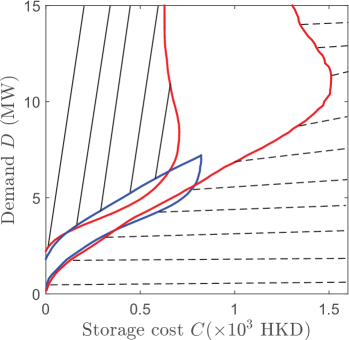
Figure 9: (a) Equilibrium split in the homogeneous case; (b) Equilibrium split in the heterogeneous case.

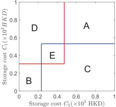
Figure 10: Equilibrium split with storage cost.

Generally, in the heterogeneous case, we see that the region where supplier 2 should invest in storage is larger than the region of supplier 1. The intuition is that supplier 2 has a larger capacity of renewables, which gives her advantage in the competition. When both suppliers face the same high storage cost greater than 1000 HKD as in Figure 9, supplier 1 will not invest in storage at the equilibrium for any demand $D$ but supplier 2 may still invest in storage when the demand is high. Also, the region of only supplier 1 investing in storage and only supplier 2 investing in storage can overlap under the heterogeneous case, which means that only supplier 1 investing in storage and only supplier 2 investing in storage are both equilibria.

Next we consider the case that two heterogeneous suppliers bear different storage investment costs. We choose a certain demand ($D=4$ MW) and show the equilibrium split with respect to the storage cost of the two suppliers in Figure 10. In Figure 10, if the storage costs of supplier 1 and supplier 2 lie in Region A, neither supplier will invest in storage. In Region B, both suppliers will invest in storage. In Region D, only supplier 2 invests in storage and supplier 1 will not invest in storage. In Region C, only supplier 1 invests in storage and supplier 2 will not invest in storage. However, in Region E, only supplier 1 investing in storage and only supplier 2 investing in storage, are both equilibria.

XV Appendix: Proofs of Stage III

To prove Proposition 1, we will discuss the following two cases and analyze the objective function of Problem (4) based on linear functions. For notation simplicity, we omit the superscript $m,t$ in the corresponding variables and parameters.

• If $p_{1}=p_{2}=p$, we rewrite the objective function (4a) as

  $$(P_{g}-p)(x_{1}+x_{2}).$$ (28)

  Since $P_{g}-p>0$, the optimal value is achieved at the maximum value of $x_{1}+x_{2}$, i.e., $\min(D,y_{1}+y_{2})$ according to the constraints (4b) and (4c).

• If $p_{1}\neq p_{2}$, we assume $p_{1}>p_{2}$ without loss of generality. We rewrite the objective function (4a) as

  $$(P_{g}-p_{2})(x_{1}+x_{2})+(p_{1}-p_{2})x_{1}.$$ (29)

  Since $P_{g}-p_{2}>0$ and $p_{1}-p_{2}>0$, the optimal value is achieved at the maximum value of $x_{1}+x_{2}$ and the maximum value of $x_{1}$ as follows:

  $$x_{1}^{*}+x_{2}^{*}=\min(D,y_{1}+y_{2}),$$ (30)

  $$x_{1}^{*}=\min(y_{1},D).$$ (31)

  Then, we obtain the optimal solution $x_{2}^{*}=\min(D,y_{1}+y_{2})-\min(y_{1},D)$, which is equivalent to $x_{2}^{*}=\min(D-\min(y_{1},D),y_{2})$.

Combining the above two cases, we have Proposition 1 proved. ∎

Remark 1: Proposition 1 can be easily extended to the oligopoly case with more than 2 suppliers.

Remark 2: Given the other supplier $-i$’s bidding price $p_{-i}$ and bidding quantity $y_{-i}$, the supplier $i$’s payoff function generally is not continuous in price $p_{i}$ at $p_{i}=p_{-i}$ due to the discontinuous change of the optimal capacity $x_{i}^{*}$. This shows that given the other supplier $-i$’s decisions, supplier $i$’s payoff function generally is discontinuous.

XVI Appendix: Proofs of Stage II

XVI-A Proof of Theorem 1

To prove Theorem 1, the key step is to show that given price $p_{i}$, the revenue function $\pi_{i}^{R}\left(p_{i},x_{i}^{*}(\bm{p},\bm{y}),\bm{\varphi}\right)$ of supplier $i$ with respect to $x_{i}^{*}(\bm{p},\bm{y})$ is increasing on the interval $(0,y_{i}^{*})$ and decreasing on the interval $(y_{i}^{*},+\infty)$. Then, combined with Proposition 1, we can prove that $y_{i}^{*}$ will be the weakly dominant strategy for the bidding quantity. We discuss the weakly dominant strategy for supplier $i$ with $\varphi_{i}=1$ and $\varphi_{i}=0$, respectively.

XVI-A1 Case of $\varphi_{i}=1$

We will prove that the weakly dominant strategy of bidding quantity for the with-storage supplier $i$ (i.e., $\varphi_{i}=1$) is $y_{i}^{*}\left(p_{i},\varphi_{i}\right)=\mathbb{E}[X_{i}]$. Given any price $p_{i}\leq\bar{p}<\lambda$, the function $\pi_{i}^{R}\left(p_{i},x_{i}^{*}(\bm{p},\bm{y}),\bm{\varphi}\right)$ with respect to $x_{i}^{*}(\bm{p},\bm{y})$ is linearly increasing on the interval $(0,\mathbb{E}[X_{i}])$ and linearly decreasing on the interval $(\mathbb{E}[X_{i}],+\infty)$. Thus, given any price $p_{i}$, we always have

$$\pi_{i}^{R}\left(p_{i},x_{i}^{*}(\bm{p},\bm{y}),\bm{\varphi}\right)\leq\pi_{i}^{R}\left(p_{i},\mathbb{E}[X_{i}],\bm{\varphi}\right)$$ (32)

Then, we discuss a total of three cases to show that with-storage supplier’s revenue cannot be better off if he chooses strategy $y_{i}$ other than $y_{i}^{*}\left(p_{i},\varphi_{i}\right)=\mathbb{E}[X_{i}]$. For notation simplicity, we use $y_{i}^{*}$ to represent $y_{i}^{*}\left(p_{i},\varphi_{i}\right)$ in the later discussion.

(a) If $y_{i}<y_{i}^{*}=\mathbb{E}[X_{i}]$, according to Proposition 1, we have

$$x_{i}^{*}(\bm{p},({y}_{i},y_{-i}))\leq x_{i}^{*}(\bm{p},({y}_{i}^{*},y_{-i}))\leq\mathbb{E}[X_{i}],~{}\text{for~{}any~{}}y_{-i},$$ (33)

which (according to (32)) implies

$$\pi_{i}^{R}\left(p_{i},x_{i}(\bm{p},({y}_{i},y_{-i})),\bm{\varphi})\leq\pi_{i}(p_{i},x_{i}(\bm{p},({y}_{i}^{*},y_{-i})),\bm{\varphi}\right).$$ (34)

(b) If $y_{i}>y_{i}^{*}=\mathbb{E}[X_{i}]$ and $x_{i}^{*}(\bm{p},({y}_{i},y_{-i}))>\mathbb{E}[X_{i}]$, according to Proposition 1, we have

$$x_{i}^{*}(\bm{p},({y}_{i}^{*},y_{-i}))=\mathbb{E}[X_{i}],$$

which (according to (32)) implies

$$\pi_{i}^{R}(p_{i},x_{i}^{*}(\bm{p},({y}_{i},y_{-i})),\bm{\varphi})\leq\pi_{i}^{R}(p_{i},\mathbb{E}[X_{i}],\bm{\varphi})=\pi_{i}^{R}(p_{i},x_{i}^{*}(\bm{p},({y}_{i}^{*},y_{-i})),\bm{\varphi}).$$

(c) If $y_{i}>y_{i}^{*}=\mathbb{E}[X_{i}]$ and $x_{i}^{*}(\bm{p},({y}_{i},y_{-i}))\leq\mathbb{E}[X_{i}]$, according to Proposition 1, we have

$$x_{i}^{*}(\bm{p},({y}_{i},y_{-i}))=x_{i}^{*}(\bm{p},({y}_{i}^{*},y_{-i})),$$

which implies

$$\pi_{i}^{R}(p_{i},x_{i}^{*}(\bm{p},({y}_{i},y_{-i})),\bm{\varphi})=\pi_{i}^{R}(p_{i},x_{i}^{*}(\bm{p},({y}_{i}^{*},y_{-i})),\bm{\varphi}).$$

Combining the above three conditions (a)-(c), we complete the proof that $y_{i}^{*}=\mathbb{E}[X_{i}]$ if $\varphi_{i}=1$.

XVI-A2 Case of $\varphi_{i}=0$

We prove the weakly dominant strategy of bidding quantity for the without-storage supplier $i$ (i.e., $\varphi_{i}=0$) is $y_{i}^{*}=F_{i}^{-1}(\frac{p_{i}}{\lambda})$. We take the derivative of $\pi_{i}^{R}\left(p_{i},x_{i}^{*}(\bm{p},\bm{y}),\bm{\varphi}\right)$ with respect to $x_{i}^{*}(\bm{p},\bm{y})$ and give any $p_{i}>0$, it is easy to show that the function $\pi_{i}^{R}\left(p_{i},x_{i}^{*}(\bm{p},\bm{y}),\bm{\varphi}\right)$ is increasing on the interval interval $(0,F_{i}^{-1}(\frac{p_{i}}{\lambda}))$ and decreasing on the interval $(F_{i}^{-1}(\frac{p_{i}}{\lambda}),+\infty)$. Thus, given any price $p_{i}$, we always have

$$\pi_{i}^{R}\left(p_{i},x_{i}^{*}(\bm{p},\bm{y}),\bm{\varphi}\right)\leq\pi_{i}^{R}\left(p_{i},F_{i}^{-1}(\frac{p_{i}}{\lambda}),\bm{\varphi}\right).$$ (35)

Then, we can follow the proof step for $y_{i}^{*}$ in the case of $\varphi_{i}=1$ and prove that $y_{i}^{*}=F_{i}^{-1}(\frac{p_{i}}{\lambda})$ for supplier $i$ with $\varphi_{i}=0$. ∎

XVI-B Proof of Proposition 2

We verify the pure price equilibrium according to Definition 2 that the supplier cannot be better off if he deviates unilaterally. Towards this end, note that for supplier $i$ with or without storage, the revenue function $\pi_{i}^{R}\left(p_{i},x_{i}^{*}(\bm{p},\bm{y}),\bm{\varphi}\right)$ is strictly increasing with respect to both the price $p_{i}$ and the selling quantity $x_{i}^{*}(\bm{p},\bm{y})$ that is in the range $[0,y_{i}^{*}(p_{i},\varphi_{i})]$ (without considering the other supplier’s coupled decisions). We will discuss the three types of subgames respectively.

XVI-B1 The type $\text{S}_{0}\text{S}_{0}$ (i.e., $\sum_{i}\varphi_{i}=0$)

We first prove that when $D\geq\sum_{i}y_{i}^{*}(\bar{p},{\varphi}_{i})$, $p_{1}=p_{2}=\bar{p}$ is a pure price equilibrium and show that this pure price equilibrium is unique. Then, we show that when $D<\sum_{i}y_{i}^{*}(\bar{p},{\varphi}_{i})$, there exists no pure price equilibrium.

(a) The case of $D\geq\sum_{i}y_{i}^{*}(\bar{p},{\varphi}_{i})$.

We first prove that when $D\geq\sum_{i}y_{i}^{*}(\bar{p},{\varphi}_{i})$, $p_{1}=p_{2}=\bar{p}$ is a pure price equilibrium. When $p_{1}=p_{2}=\bar{p}$, according to Proposition 1, the total selling energy quantities of supplier 1 and supplier 2 satisfy

$$\sum_{i}x_{i}^{*}\left((\bar{p},\bar{p}),({y}_{1}^{*}(\bar{p},{\varphi}_{1}),{y}_{2}^{*}(\bar{p},{\varphi}_{2}))\right) =\min(D,{y}_{1}^{*}(\bar{p},{\varphi}_{1})+{y}_{2}^{*}(\bar{p},{\varphi}_{2}))$$ (36)

$$={y}_{1}^{*}(\bar{p},{\varphi}_{1})+{y}_{2}^{*}(\bar{p},{\varphi}_{2}).$$ (37)

Since $x_{i}^{*}(\bm{p},\bm{y})\leq y_{i}^{*}(p_{i},\varphi_{i})$ always holds for any $i=1,2$, based on (37), we have

$$x_{i}\triangleq x_{i}^{*}((\bar{p},\bar{p}),({y}_{1}^{*}(\bar{p},{\varphi}_{1}),{y}_{2}^{*}(\bar{p},{\varphi}_{2})))={y}_{i}^{*}(\bar{p},{\varphi}_{i}).$$ (38)

We will show that both suppliers cannot be better off if they deviate from such a bidding strategy. Without loss of generality, if supplier $1$ bids a price $p_{1}^{\prime}<\bar{p}$ unilaterally, according to Proposition 1, we have

$$x_{1}^{\prime}\triangleq{x}_{1}^{*}(({p}_{1}^{\prime},\bar{p}),({y}_{1}^{*}(p_{1}^{\prime},{\varphi}_{1}),{y}_{2}^{*}(\bar{p},{\varphi}_{2})) =\min\left\{D,{y}_{1}^{*}(p_{1}^{\prime},{\varphi}_{1})\right\}$$ (39)

$$={y}_{1}^{*}(p_{1}^{\prime},{\varphi}_{1})$$ (40)

$$<x_{1}.$$ (41)

Since the revenue function $\pi_{i}^{R}\left(p_{i},x_{i}^{*}(\bm{p},\bm{y}),\bm{\varphi}\right)$ is strictly increasing with respect to the price $p_{i}$ and the selling quantity $x_{i}^{*}(\bm{p},\bm{y})\leq y^{*}$, we have

$$\pi_{1}^{R}\left(p_{1}^{\prime},x_{1}^{\prime},\bm{\varphi}\right)<\pi_{1}^{R}\left(\bar{p},x_{1},\bm{\varphi}\right),$$ (42)

which shows that supplier 1’s revenue decreases if he deviates from the price $\bar{p}$. This proves that $p_{1}=p_{2}=\bar{p}$ is a pure price equilibrium.

Next, we show that this equilibrium is unique. Without loss of generality, suppose that supplier 1 bids a price $p_{1}^{\prime}<\bar{p}$ while the other supplier bids a price $p_{2}^{\prime}\leq\bar{p}$. Since $D\geq\sum_{i}y_{i}^{*}(\bar{p},{\varphi}_{i})$, according to Proposition 1, each supplier’s maximum bidding quantity will be sold out and we have

$$x_{1}^{*}(\bm{p}^{\prime},\bm{y}^{*}(\bm{p}^{\prime},\bm{\varphi}))=y_{1}^{*}(p_{1}^{\prime},\varphi_{1})\leq y_{1}^{*}(\bar{p},\varphi_{1}).$$ (43)

Therefore, supplier 1 can always increase his price $p_{i}^{\prime}$ to $\bar{p}$, which will increase his revenue due to the increased price and non-decreasing selling quantity. Thus, any price pair $(p_{1},p_{2})\neq(\bar{p},\bar{p})$ can’t be an equilibrium.

(b) Case of $0<D<\sum_{i}y_{i}^{*}(\bar{p},{\varphi}_{i})$ .

We will assume that both suppliers bid the pure prices and will discuss a total of three cases in the following to show that no pure price strategy can be an equilibrium.

First, suppliers’ bidding prices are not equal, and we assume $p_{i}<p_{-i}$ without loss of generality. the lower-price supplier can always increase the price by a small $\varepsilon>0$ such that $p_{i}^{\prime}=p_{i}+\varepsilon<p_{-i}$. Then, the bidding price $p_{i}^{\prime}>p_{i}$ and the selling quantity at $p_{i}^{\prime}$ denoted as ${x}_{i}^{\prime}$ satisfies ${x}_{i}^{\prime}=\min\left\{D,y_{i}^{*}(p_{i}+\varepsilon,\varphi_{i})\right\}\geq x_{i}=\min\left(D,y_{i}^{*}(p_{i},\varphi_{i})\right)$. In this case, we denote the revenue at the original price $p_{i}$ as $\pi_{i}$, and the revenue at the price $p_{i}^{\prime}$ as $\pi_{i}^{\prime}$. We have $\pi_{i}^{\prime}>\pi_{i}$ since $p_{i}^{\prime}>p_{i}$ and ${x}_{i}^{\prime}\geq x_{i}$. Thus, the unequal bidding price cannot be an equilibrium.

Second, two suppliers bid the same positive price, i.e., $p_{1}=p_{1}=p>0$. Based on Proposition 1, the selling quantities of two suppliers satisfy the following condition

$$\sum_{i}x_{i}^{*}(\bm{p},\bm{y}^{*}(\bm{p},\bm{\varphi}))=\min(D,y_{1}^{*}({p},\varphi_{1})+y_{2}^{*}({p},\varphi_{2})).$$ (44)

For simplicity, we denote the original selling quantity of supplier 1 and supplier 2 as $x_{1}$ and $x_{2}$, respectively when $p_{1}=p_{1}=p>0$. Then we discuss two cases (i) and (ii).

• (i) When $D<y_{1}^{*}({p},\varphi_{1})+y_{2}^{*}({p},\varphi_{2})$, we have

  $$x_{1}+x_{2}=D.$$ (45)

  In this case, if supplier 1 reduces the price by a small $\varepsilon_{1}>0$ to a price $p_{1}^{\prime}=p-\varepsilon_{1}$ unilaterally, we have

  $$x_{1}^{\prime}\triangleq{x}_{1}^{*}(({p}-\varepsilon_{1},{p}),(y_{1}^{*}({p-\varepsilon_{1}},\varphi_{1}),y_{2}^{*}({p},\varphi_{2}))=\min\left\{D,y_{1}^{*}({p-\varepsilon_{1}},\varphi_{1})\right\}.$$ (46)

  If supplier $2$ reduces the price by a small $\varepsilon_{2}>0$ to a price $p_{2}^{\prime}=p-\varepsilon_{2}$ unilaterally , we have

  $$x_{2}^{\prime}\triangleq{x}_{2}^{*}(({p},{p}-\varepsilon_{2}),(y_{1}^{*}({p},\varphi_{1}),y_{2}^{*}({p-\varepsilon_{2}},\varphi_{2}))=\min\left\{D,y_{2}^{*}(p-\varepsilon_{2},\varphi_{2})\right\}.$$ (47)

  We choose small $\varepsilon_{1}$ and $\varepsilon_{2}$ such that $D<y_{1}^{*}({p}-\varepsilon_{1},\varphi_{1})+y_{2}^{*}({p}-\varepsilon_{2},\varphi_{2})$ holds. Then, we have

  $$x_{1}^{\prime}+x_{2}^{\prime}=\min\left\{D,y_{1}^{*}({p-\varepsilon_{1}},\varphi_{1})\right\}+\min\left\{D,y_{2}^{*}(p-\varepsilon_{2},\varphi_{2})\right\}.$$ (48)

  Combining (45) and (48), we see that at least one supplier $i$ can always reduce the price by a small $\varepsilon_{i}>0$ unilaterally such that the selling quantity increases by

  $$x_{i}^{\prime}-x_{i}>\frac{1}{2}\min(D,y_{1}^{*}({p-\varepsilon_{1}},\varphi_{1}),y_{2}^{*}({p-\varepsilon_{2}},\varphi_{2})).$$

  Since we can choose a sufficiently small $\varepsilon_{i},\forall i=1,2$, the revenue $\pi_{i}$ will increase due to the increased selling quantity $x_{i}^{\prime}-x_{i}$ (with an upward jumping).

• (ii) When $y_{1}^{*}({p},\varphi_{1})+y_{2}^{*}({p},\varphi_{2})\leq D<y_{1}^{*}(\bar{p},\varphi_{1})+y_{2}^{*}(\bar{p},\varphi_{2})$, we have

  $$x_{1}+x_{2}=y_{1}^{*}({p},\varphi_{1})+y_{2}^{*}({p},\varphi_{2}).$$ (49)

  Both suppliers can sell out the bidding quantities completely as follows.

  $$x_{1}=y_{1}^{*}({p},\varphi_{1}),~{}x_{2}=y_{2}^{*}({p},\varphi_{2}).$$ (50)

  Note that $D-y_{2}^{*}({p},\varphi_{2})\geq y_{1}^{*}({p},\varphi_{1})=x_{1}$. Supplier $1$ can always increase his price $p$ to $p^{\prime}=\bar{p}>p$ unilaterally, and $x_{1}^{\prime}=\min(y_{1}^{*}({p^{\prime}},\varphi_{1}),D-y_{2}^{*}({p},\varphi_{2}))$. Since we also have $y_{1}^{*}({p^{\prime}},\varphi_{1})\geq y_{1}^{*}({p},\varphi_{1})=x_{1}$, supplier $1$’s obtained demand $x_{1}^{\prime}$ at $p^{\prime}$ will not decrease, i.e., $x_{i}^{\prime}\geq x_{i}$. Thus, the revenue of supplier $i$ after increasing the price will also increase.

In summary, when two suppliers bid the same positive price, one supplier can always deviate so as to obtain a higher revenue, which shows that the equal positive bidding prices cannot be pure price equilibrium.

Third, both suppliers bid the price at zero: $p_{1}=p_{2}=0$. In this case, both suppliers have zero revenues: $\pi_{1}^{R}=\pi_{2}^{R}=0$. Note that both without-storage suppliers will also bid the zero quantity $y_{i}^{*}(p_{i},\varphi_{i})=0$ as shown in Theorem 1. Thus, any supplier $i$ can always set a positive price $p_{i}^{\prime}>0$ to obtain the positive demand since the other supplier bid zero quantity. This makes his revenue $\pi_{1}^{R^{\prime}}>0$ after increasing the price. There, the pure price strategy $p_{1}=p_{2}=0$ cannot be the equilibrium

So far, for the case of $0<D<\sum_{i}y_{i}^{*}(\bar{p},{\varphi}_{i})$ , we have discussed all the three cases of the pure price strategies but none of them is an equilibrium. Thus, there exists no pure price equilibrium when $0<D<\sum_{i}y_{i}^{*}(\bar{p},{\varphi}_{i})$.

XVI-B2 The type $\text{S}_{1}\text{S}_{0}$ (i.e., $\sum_{i}\varphi_{i}=1$)

Following the same arguments as in the type $\text{S}_{0}\text{S}_{0}$, we can first prove that when $D\geq\sum_{i}y_{i}^{*}(\bar{p},{\varphi}_{i})$, $p_{1}=p_{2}=\bar{p}$ is a pure price equilibrium and show that this pure price equilibrium is unique. Furthermore, we can show that when $D<\sum_{i}y_{i}^{*}(\bar{p},{\varphi}_{i})$, there exists no pure price equilibrium.

XVI-B3 The type $\text{S}_{1}\text{S}_{1}$ (i.e., $\sum_{i}\varphi_{i}=2$)

The results have been proved in the paper [17].

In conclusion, we have Proposition 2 proved.

XVI-C Proof of Theorem 2

We prove Theorem 2 based on Lemma 1 that has been shown in [17]. However, based on Lemma 1, deriving the mixed price equilibrium in our model is still not straightforward compared with [17]. That is because, in [17], supplier’s bidding quantity is upper-bounded by his deterministic production quantity, while in our model, without-storage supplier’s bidding quantity is upper-bounded by a function of price. The difference significantly increases the complexity of the analysis in our work.

To prove Theorem 2, we will utilize a basic property of mix strategy equilibrium as shown in Lemma 2[41]. In Lemma 2, we use $\pi_{i}^{RM}(\mu_{i},\mu_{-i},\bm{\varphi})$ to denote the expected revenue of supplier $i$ at any arbitrary mixed price strategy $(\mu_{1},\mu_{2})$, which is defined as follows.

$$\pi_{i}^{RM}(\mu_{i},\mu_{-i},\bm{\varphi})=\int_{{[0,\bar{p}]}^{2}}\pi_{i}^{R}(p_{i},{x}_{i}^{*}((p_{i},{p}_{-i}),\bm{y}^{*}(p_{i},p_{-i})),\bm{\varphi})d(\mu_{i}(p_{i})\times{\mu}_{-i}({p}_{-i}))$$

Lemma 2.

$\pi_{i}^{RM}(p_{i},\mu_{-i}^{*},\bm{\varphi})=\pi_{i}^{RE}(\bm{\varphi})$, for all $p_{i}\in[l,\bar{p}]$, where $\pi_{i}^{RE}$ is the equilibrium revenue [41].

Lemma 2 shows that the equilibrium revenue $\pi_{i}^{RE}$ of supplier $i$ is equal to the expected revenue when he plays any pure strategy $p_{i}$ in the support, i.e., $p_{i}\in[l,\bar{p}]$, against the mixed strategy $\mu_{-i}^{*}$ of the other supplier at the equilibrium.

Based on Lemma 1 and Lemma 2, we will characterize the equilibrium revenue $\pi_{i}^{RE}$ as well as the CDF of the mixed price equilibrium $F_{i}^{e}(p)$ using the lower support $l$ over $p\in[l,\bar{p})$. We make the analysis of the with-storage supplier (i.e., $\varphi_{i}=1$) and without-storage supplier (i.e., $\varphi_{i}=0$) as follows.

XVI-C1 With-storage supplier $i$ (i.e., $\varphi_{i}=1$)

For supplier $i$, based on Lemma 2, the equilibrium revenue $\pi_{i}^{RE}$ can be characterized by the expected revenue when he plays any pure strategy $p_{i}\in[l,\bar{p})$ against the mixed strategy of supplier $-i$ (with CDF $F_{-i}^{e}$ and PDF $f_{-i}^{e}$) at the equilibrium as follows

$$\pi_{i}^{RE}(\bm{\varphi}) =\pi_{i}^{RM}(p_{i},\mu_{-i}^{*},\bm{\varphi})$$

$$=\underbrace{p_{i}\min(D,\mathbb{E}[X_{i}])\cdot(1-F_{-i}^{e}(p_{i}))}_{p_{i}\leq p_{-i}}$$

$$~{}~{}~{}~{}+\underbrace{p_{i}\int_{l}^{p_{i}}\min\left(D-\min(y_{-i}^{*}(p_{-i},\varphi_{-i}),D),\mathbb{E}[X_{i}]\right)\cdot f_{-i}^{e}(p_{-i})dp_{-i}}_{p_{i}>p_{-i}}.$$ (51)

Note that in (51), $D-\min(y_{-i}^{*}(p_{-i},\varphi_{-i}),D)\leq\mathbb{E}[X_{i}]$ will always hold for any $p_{-i}\in[l,\bar{p}]$, i.e., $D-\min(y_{-i}^{*}(l,\varphi_{-i}),D)\leq\mathbb{E}[X_{i}]$, or

$$D\leq\mathbb{E}[X_{i}]+y_{-i}^{*}(l,\varphi_{-i}).$$ (52)

This helps us simplify the second part “$p_{i}>p_{-i}$" in (51). We can prove this by contradiction as follows. If $D-\min(y_{-i}^{*}(l,\varphi_{-i}),D)>\mathbb{E}[X_{i}]$, there exists a small $\varepsilon>0$ such that $D-\min(y_{-i}^{*}(l+\varepsilon,\varphi_{-i}),D)>\mathbb{E}[X_{i}]$ still holds. Based on (51), we have

$$\pi_{i}^{RE}=\pi_{i}^{RM}(l,\mu_{-i}^{*},\bm{\varphi})={l\cdot\min(D,\mathbb{E}[X_{i}])},$$ (53)

and for any $\varepsilon>0$,

$$\pi_{i}^{RE}(\bm{\varphi}) =\pi_{i}^{RM}(l+\varepsilon,\mu_{-i}^{*},\bm{\varphi})$$

$$={(l+\varepsilon)\cdot\min(D,\mathbb{E}[X_{i}])(1-F_{-i}^{e}(l+\varepsilon))}+{(l+\varepsilon)\int_{l}^{l+\varepsilon}\mathbb{E}[X_{i}]\cdot f_{-i}^{e}(p_{-i})dp_{-i}}$$

$$={(l+\varepsilon)\cdot\min(D,\mathbb{E}[X_{i}])(1-F_{-i}^{e}(l+\varepsilon))}+{(l+\varepsilon)\cdot\mathbb{E}[X_{i}]\cdot F_{-i}^{e}(l+\varepsilon)}$$

$$\geq(l+\varepsilon)\cdot\min(D,\mathbb{E}[X_{i}]).$$ (54)

Then, we can see that $\eqref{eq:pif2}$ and $\eqref{eq:pif1}$ contradict with each other, and thus $D-\min(y_{-i}^{*}(p_{-i},\varphi_{-i}),D)\leq\mathbb{E}[X_{i}]$ will always hold for $p_{2}\in[l,\bar{p}]$, which enables us to simplify (51).

Since $\pi_{i}^{RE}(\bm{\varphi})=\pi_{i}^{RM}(p_{i},\mu_{-i}^{*},\bm{\varphi})$ is constant over $p_{i}\in[l,\bar{p})$, the derivative of $\pi_{i}^{RM}(p_{i},\mu_{-i}^{*},\bm{\varphi})$ with respect to $p_{i}$ is zero over $p_{i}\in[l,\bar{p})$, i.e.,

$$\frac{\partial\pi_{i}^{RM}(p_{i},\mu_{-i}^{*},\bm{\varphi})}{\partial p_{i}}= {\min(D,\mathbb{E}[X_{i}])(1-F_{-i}^{e}(p_{i}))}+p_{i}\min(D,\mathbb{E}[X_{i}])(-f_{-i}^{e}(p_{i}))$$

$$+ {\int_{l}^{p_{i}}\left(D-\min(y_{-i}^{*}(p_{-i}),D)\right)f_{-i}^{e}(p_{-i})dp_{-i}}+{{p_{i}}\left(D-\min(y_{-i}^{*}(p_{i},\varphi_{-i}),D)\right)f_{-i}^{e}(p_{i})}$$

$$= 0.$$ (55)

Combining (XVI-C1) with (51), we have the PDF of mixed price strategy at the equilibrium for without-storage supplier ${-i}$’s as follows.

$$f_{-i}^{e}(p)=\frac{\pi_{i}^{RE}(\bm{\varphi})}{p^{2}\cdot\min\{y_{-i}^{*}(p,\varphi_{-i}),D\}-p^{2}\cdot[D-\mathbb{E}{[X_{i}]}]^{+}},$$ (56)

which is characterized by the equilibrium revenue $\pi_{i}^{RE}$ of supplier $i$.

XVI-C2 Without-storage supplier $i$ (i.e., $\varphi_{i}=0$)

For supplier $i$ without storage, similarly, based on Lemma 2, the equilibrium revenue $\pi_{i}^{RE}(\bm{\varphi})$ can be characterized by the expected revenue when he plays any pure strategy $p_{i}\in[l,\bar{p})$ against the mixed strategy of supplier ${-i}$ (with CDF $F_{-i}^{e}$) at the equilibrium as follows

$$\pi_{i}^{RE}(\bm{\varphi})= \pi_{i}^{RM}(p_{i},\mu_{-i}^{*},\bm{\varphi})$$ (57)

$$= \underbrace{\pi_{i}^{R}(p_{i},\min\left(D,y_{i}^{*}(p_{i},\varphi_{i}),\bm{\varphi}\right))\cdot(1-F_{-i}^{e}(p_{i}))}_{p_{i}\leq p_{-i}}$$

$$+\underbrace{\pi_{i}^{R}\left(p_{i},\min(D-\min(\mathbb{E}[X_{-i}],D),y_{i}^{*}(p_{i},\varphi_{i})),\bm{\varphi}\right)\cdot F_{-i}^{e}(p_{i})}_{p_{i}>p_{-i}}.$$ (58)

Similarly, we have that $D-\min(\mathbb{E}[X_{-i}],D)\leq y_{i}^{*}(p_{i},\varphi_{i})$ always holds for any $p_{i}\in[l,\bar{p}]$. Then, according to (58), we have the PDF of the mixed price strategy at the equilibrium for the with-storage supplier $-i$ as follows.

$$F_{-i}^{e}(p)=\frac{\pi_{i}^{R}\left(p,\min\{y_{i}^{*}(p,\varphi_{i}),D\},\bm{\varphi}\right)-\pi_{i}^{RE}(\bm{\varphi})}{\pi_{i}^{R}\left(p,\min\{y_{i}^{*}(p,\varphi_{i}),D\},\bm{\varphi}\right)-\pi_{i}^{R}\left(p,[D-\mathbb{E}[X_{-i}]]^{+},\bm{\varphi}\right)},$$ (59)

which is characterized by the equilibrium revenue $\pi_{i}^{RE}$ of supplier $i$.

In conclusion, if $\varphi_{i}=1$, we have

$$F_{i}^{e}(p)=\frac{\pi_{-i}^{R}\left(p,\min\{y_{-i}^{*}(p,\varphi_{-i}),D\},\bm{\varphi}\right)-\pi_{-i}^{RE}(\bm{\varphi})}{\pi_{-i}^{R}(p,\min\{y_{-i}^{*}(p,\varphi_{-i}),D\},\bm{\varphi})-\pi_{-i}^{R}(p,(D-\mathbb{E}[X_{i}])^{+},\bm{\varphi})}.$$ (60)

If $\varphi_{i}=0$, we have

$$F_{i}^{e}(p)=\int_{l}^{\bar{p}}\frac{\pi_{-i}^{RE}(\bm{\varphi})}{p^{2}\cdot\min\{y_{i}^{*}(p,\varphi_{i}),D\}-p^{2}\cdot(D-\mathbb{E}[X_{-i}])^{+}}dp.$$ (61)

for any $l\leq p<\bar{p}$.

∎

XVI-D Proof of Proposition 3

To prove Proposition 3, we first show that $F_{i}^{e}(\bar{p}^{-}\mid l_{i}^{\dagger})$ is always decreasing in $l_{i}^{\dagger},\forall i$, based on which we can prove Proposition 3 (1) by contradiction. Then, we can have Proposition 3 (2) proved directly from Lemma 1 (iii).

We now prove that $F_{i}^{e}(\bar{p}^{-}\mid l_{i}^{\dagger})$ is always decreasing with $l_{i}^{\dagger}$, for both $\varphi_{i}=1$ and $\varphi_{i}=0$.

XVI-D1 With-storage supplier $i$ (i.e, $\varphi_{i}=1$)

For the without-storage supplier $i$, according to (11), we have

$$F_{i}^{e}(\bar{p}^{-}\mid l_{i}^{\dagger})=\frac{\pi_{-i}^{R}\left(\bar{p},\min\{y_{-i}^{*}(\bar{p},\varphi_{-i}),D\},\bm{\varphi}\right)-\pi_{-i}^{RE}(\bm{\varphi})}{\pi_{-i}^{R}(\bar{p},\min\{y_{-i}^{*}(p,\varphi_{-i}),D\},\bm{\varphi})-\pi_{-i}^{R}(\bar{p},(D-\mathbb{E}[X_{i}])^{+},\bm{\varphi})}.$$ (62)

Note that the equilibrium revenue function $\pi_{-i}^{RE}(\bm{\varphi})$ (shown in Lemma 1 (iii)) is increasing in the lower support $l_{i}^{\dagger}$, and thus $F_{i}^{e}(\bar{p}^{-}\mid l_{1}^{\dagger})$ is decreasing in $l_{i}^{\dagger}$.

XVI-D2 Without-storage supplier $i$ (i.e, $\varphi_{i}=0$)

For the without-storage supplier $i$, according to (12), we have

$$F_{i}^{e}(\bar{p}^{-}\mid l_{i}^{\dagger})=\int_{l_{i}^{\dagger}}^{\bar{p}}\frac{{l_{i}^{\dagger}}\cdot\min(D,\mathbb{E}[X_{i}])}{p^{2}\cdot\min\{y_{i}^{*}(p,\varphi_{i}),D\}-p^{2}\cdot[D-\mathbb{E}[X_{i}]]^{+}}dp.$$ (63)

We take the first-order derivative of $F_{i}^{e}(\bar{p}^{-}\mid l_{i}^{\dagger})$ with respect to $l_{i}^{\dagger}$ and obtain

$$\frac{\partial F_{i}^{e}(\bar{p}^{-}\mid l_{i}^{\dagger})}{\partial l_{i}^{\dagger}} =\int_{l_{i}^{\dagger}}^{\bar{p}}\frac{\min(D,\mathbb{E}[X_{i}])}{p^{2}\cdot\min\{y_{i}^{*}(p,\varphi_{i}),D\}-p^{2}\cdot(D-\mathbb{E}[X_{i}])^{+}}dp$$

$$~{}~{}~{}~{}~{}~{}~{}-\frac{\min(D,\mathbb{E}[X_{i}])}{{l_{i}^{\dagger}}\cdot\min\{y_{i}^{*}(l_{i}^{\dagger},\varphi_{i}),D\}-{l_{i}^{\dagger}}\cdot(D-\mathbb{E}[X_{i}])^{+}}.$$ (64)

Further, we take the derivative of (64) with respect to $l_{i}^{\dagger}$ again and have

$$\frac{\partial^{2}F_{i}^{e}(\bar{p}^{-}\mid l_{i}^{\dagger})}{\partial{l_{i}^{\dagger}}^{2}}=-\frac{1}{{l_{i}^{\dagger}}}\cdot\frac{\partial\frac{\min(D,\mathbb{E}[X_{i}])}{\min\{y_{i}^{*}(l_{i}^{\dagger},\varphi_{i}),D\}-(D-\mathbb{E}[X_{i}])^{+}}}{\partial l_{i}^{\dagger}}.$$ (65)

Note that $\frac{\min(D,\mathbb{E}[X_{i}])}{\min\{y_{i}^{*}(l_{i}^{\dagger},\varphi_{i}),D\}-(D-\mathbb{E}[X_{i}])^{+}}$ decreases in $l_{i}^{\dagger}$ because $y_{i}^{*}(l_{i}^{\dagger},\varphi_{i})$ increases in $l_{i}^{\dagger}$. Thus, we always have

$$\frac{\partial^{2}F_{i}^{e}(\bar{p}^{-}\mid l_{i}^{\dagger})}{\partial{l_{i}^{\dagger}}^{2}}\geq 0,$$ (66)

which shows that $\frac{\partial F_{i}^{e}(\bar{p}^{-}\mid l_{i}^{\dagger})}{\partial l_{i}^{\dagger}}$ is non-decreasing with $l_{i}^{\dagger}$. Then, we choose $l_{i}^{\dagger}=\bar{p}$ and have

$$\frac{\partial F_{i}^{e}(\bar{p}^{-}\mid l_{i}^{\dagger})}{\partial l_{i}^{\dagger}} =-\frac{\min(D,\mathbb{E}[X_{i}])}{{\bar{p}}\cdot\min\{y_{i}^{*}(\bar{p},\varphi_{i}),D\}-{\bar{p}}\cdot(D-\mathbb{E}[X_{i}])^{+}}$$

$$<0,$$

which holds for all $l_{i}^{\dagger}\leq\bar{p}$. The reason is that $D<\mathbb{E}[X_{i}]+y_{i}^{*}(\bar{p},\varphi_{i})$ in the subgame $\text{S}_{1}\text{S}_{0}$ without the pure price equilibrium. Therefore, we have that ${F_{i}^{e}(\bar{p}^{-}\mid l_{i}^{\dagger})}$ decreases with $l_{i}^{\dagger}$.

Till now, we have shown that $F_{i}^{e}(\bar{p}^{-}\mid l_{i}^{\dagger})$ is always decreasing in $l_{i}^{\dagger}$ for both $\varphi_{i}=1$ and $\varphi_{i}=0$. Then, we can prove Proposition 3 (1) by contradiction. According to Lemma 1 (iii), if $F_{i}^{e}(\bar{p}^{-}\mid l_{i}^{\dagger})=1$ has a solution $l_{i}^{\dagger*}$ for both suppliers $i=1,2$, either $l=\max(l_{1}^{\dagger*},l_{2}^{\dagger*})$ or $l=\min(l_{1}^{\dagger*},l_{2}^{\dagger*})$ will hold. If $l=\min(l_{1}^{\dagger*},l_{2}^{\dagger*})$, without loss of generality, we assume $l_{1}^{\dagger*}<l_{2}^{\dagger*}$ and $l=l_{1}^{\dagger*}$. Note that $F_{1}^{e}(\bar{p}^{-}\mid l_{1}^{\dagger*})=1$ and hence $F_{2}^{e}(\bar{p}^{-}\mid l_{2}^{\dagger*})=1$. Since $F_{2}^{e}(\bar{p}^{-}\mid l_{2}^{\dagger})$ is decreasing with $l_{2}^{\dagger}$, then $F_{2}^{e}(\bar{p}^{-}\mid l_{1}^{\dagger*})>1$, which is a contradiction of the CDF. Therefore, we can only choose $l=\max(l_{1}^{\dagger*},l_{2}^{\dagger*})$ and we have Proposition 3 (1) proved. Furthermore, according to Lemma 1 (iii), we have that $F_{i}^{e}(\bar{p}^{-})=1$  is true for at least one of the suppliers. Thus, if we have only one solution of $l_{i}^{\dagger}$ among $i=1$ and $i=2$, it must be the equilibrium lower support, which has Proposition 3 (2) proved. ∎

XVI-E Proof of Theorem 3

We first prove that $\pi_{i}^{RE}>\pi_{-i}^{RE}$ always holds for a general distribution for the renewable generation $X_{i}$ if $\varphi_{i}=1$, $\varphi_{-i}=0$ and $\mathbb{E}[X_{i}]=\mathbb{E}{[X_{-i}]}$. Then, we consider the case that $X_{-i}$ follows a uniform distribution.

XVI-E1 A general distribution for $X_{i}$

We consider the cases of pure price equilibrium and mixed price equilibrium respectively, and characterize suppliers’ revenue as follows.

(a) The case with pure price equilibrium: According to Proposition 2 and Lemma 1 (ii), we have

$$\pi_{i}^{RE}(\bm{\varphi})=\left\{\begin{aligned} &\bar{p}\min(\mathbb{E}[X_{i}],D),~{}\text{if}~{}\varphi_{i}=1,\\ &\pi_{i}^{R}(\bar{p},\min(D,y_{i}^{*}(\bar{p},\varphi_{i})),\bm{\varphi}),~{}\text{if}~{}\varphi_{i}=0.\end{aligned}\right.$$ (67)

Note that $D\geq\mathbb{E}[X_{i}]+y_{i}^{*}(\bar{p},\varphi_{i})$ when there is the pure price equilibrium. Therefore, if $\varphi_{i}=1$ and $\varphi_{-i}=0$, we have

$$\pi_{i}^{RE}(\bm{\varphi}) =\bar{p}\mathbb{E}[X_{i}].$$ (68)

$$\pi_{-i}^{RE}(\bm{\varphi}) =\pi_{-i}^{R}(\bar{p},y_{-i}^{*}(\bar{p},\varphi_{-i}),\bm{\varphi})$$ (69)

$$=\lambda\int_{0}^{F_{-i}^{-1}(\frac{\bar{p}}{\lambda})}xf_{-i}(x)dx.$$ (70)

$$=\lambda\int_{0}^{F_{-i}^{-1}(\frac{\bar{p}}{\lambda})}xdF_{-i}(x)$$ (71)

$$=\bar{p}F_{-i}^{-1}(\frac{\bar{p}}{\lambda})-\lambda\int_{0}^{F_{-i}^{-1}(\frac{\bar{p}}{\lambda})}F_{-i}(x)dx$$ (72)

$$<\bar{p}F_{-i}^{-1}(\frac{\bar{p}}{\lambda})-\bar{p}\int_{0}^{F_{-i}^{-1}(\frac{\bar{p}}{\lambda})}F_{-i}(x)dx.$$ (73)

Based on (73), we consider the following function $h(x)$ for any $p>0$ and $0\leq x<\bar{X}_{-i}$. Note that $F_{-i}^{-1}(\frac{\bar{p}}{\lambda})<\bar{X}_{-i}$ since $\bar{p}<\lambda$.

$$h(x)={p}x-p\int_{0}^{x}F_{-i}(x)dx.$$ (74)

The, we have

$$h^{\prime}(x)={p}-pF_{-i}(x)>0,$$ (75)

which shows that $h(x)$ increases in $x$. Since $F_{-i}^{-1}(\frac{\bar{p}}{\lambda})<\bar{X}_{-i}$, according to (73), we have

$$\pi_{-i}^{RE}(\bm{\varphi}) <\bar{p}\bar{X}_{-i}-\bar{p}\int_{0}^{\bar{X}_{-i}}F_{-i}(x)dx$$ (76)

$$=\bar{p}\mathbb{E}[X_{-i}]\leq\pi_{i}^{RE}(\bm{\varphi}).$$ (77)

Based on (68) and (77), if $\mathbb{E}[X_{-i}]\leq\mathbb{E}[X_{i}]$, then we always have

$$\pi_{-i}^{RE}(\bm{\varphi})<\pi_{i}^{RE}(\bm{\varphi}).$$ (78)

(b) The case without pure price equilibrium: The proof procedure is the similar to the case (a) with pure price equilibrium. The difference is to replace $\bar{p}$ into the lower support $l$, i.e.,

$$\pi_{i}^{RE}(\bm{\varphi})=\left\{\begin{aligned} &l\cdot\min(\mathbb{E}[X_{i}],D),~{}\text{if}~{}\varphi_{i}=1,\\ &\pi_{i}^{R}(l,\min(D,y_{i}^{*}(l,\varphi_{i})),\bm{\varphi}),~{}\text{if}~{}\varphi_{i}=0.\end{aligned}\right.$$ (79)

We will discuss the following two cases.

• $\mathbb{E}[X_{i}]\leq D$: If $\varphi_{i}=1$ and $\varphi_{-i}=0$, we have

  $$\pi_{i}^{RE}(\bm{\varphi}) =l\cdot\mathbb{E}[X_{i}].$$ (80)

  $$\pi_{-i}^{RE}(\bm{\varphi}) =\pi_{-i}^{R}(l,\min(D,y_{-i}^{*}(l,\varphi_{-i})),\bm{\varphi})$$ (81)

  $$\leq\pi_{-i}^{R}(l,y_{-i}^{*}(l,\varphi_{{-i}}),\bm{\varphi}).$$ (82)

  We can follow the same argument as in (a) with the pure price equilibrium to show that $\pi_{i}^{RE}>\pi_{-i}^{RE}$ if $\mathbb{E}[X_{i}]\geq\mathbb{E}[X_{-i}]$. The only difference is to replace $\bar{p}$ by $l$.

• $\mathbb{E}[X_{i}]>D$: If $\varphi_{i}=1$ and $\varphi_{-i}=0$, we have

  $$\pi_{i}^{RE}(\bm{\varphi}) =l\cdot D.$$ (83)

  $$\pi_{-i}^{RE}(\bm{\varphi}) =\pi_{-i}^{R}(l,\min(D,y_{-i}^{*}(l,\varphi_{-i})),\bm{\varphi}).$$ (84)

  • If $y_{-i}^{*}(l,\varphi_{{-i}})\leq D$, we have

    $$\pi_{-i}^{RE}(\bm{\varphi}) =\pi_{-i}^{R}(l,y_{-i}^{*}(l,\varphi_{-i}),\bm{\varphi})$$ (85)

    $$\leq ly_{-i}^{*}(l,\varphi_{{-i}})-l\int_{0}^{y_{-i}^{*}(l,\varphi_{{-i}})}F_{-i}(x)dx~{}(\text{as in}~{}\eqref{eq:proof_mcom})$$ (86)

    $$<lD$$ (87)

    $$=\pi_{i}^{RE}(\bm{\varphi}).$$ (88)

  • If $y_{-i}^{*}(l,\varphi_{{-i}})>D$, we have

    $$\pi_{-i}^{RE}(\bm{\varphi}) =\pi_{-i}^{R}(l,D,\bm{\varphi})$$ (89)

    $$=lD-\lambda\int_{0}^{D}(D-x)f_{-i}(x)dx$$ (90)

    $$<lD$$ (91)

    $$=\pi_{i}^{RE}(\bm{\varphi}).$$ (92)

Therefore, for the case (b) without pure price equilibrium, we also have that $\pi_{i}^{RE}>\pi_{-i}^{RE}$ if $\mathbb{E}[X_{i}]\geq\mathbb{E}[X_{-i}]$. Combining case (a) with the pure price equilibrium, for a general distribution of $X_{i}$, we prove that $\pi_{i}^{RE}>\pi_{-i}^{RE}$ if $\mathbb{E}[X_{i}]\geq\mathbb{E}[X_{-i}]$.

XVI-E2 Uniform distribution of $X_{-i}$

We will derive the revenues (at both pure and mixed price equilibrium) of suppliers under the uniform renewable-generation distribution. For the pure price equilibrium, it is straightforward to calculate the equilibrium revenue when there is $p_{1}=p_{2}=\bar{p}$ when $D\geq\sum_{i}y_{i}(\bar{p},\varphi_{i})$. For the case without pure price equilibrium, i.e., $D<\sum_{i}y_{i}(\bar{p},\varphi_{i})$, we will characterize the lower support for the mixed price equilibrium and characterize the equilibrium revenue based on Theorem 2 and Proposition 3.

We consider $\varphi_{i}=1$ and $\varphi_{-i}=0$. We have the PDF and CDF of the uniform distribution $X_{-i}$ as follows:

$$f_{-i}=\frac{1}{\bar{X}_{-i}},~{}F_{-i}(x)=\frac{x}{\bar{X}_{-i}}.$$ (93)

According to Theorem 1, the weakly dominant bidding quantity strategy is

$$y_{i}^{*}=\mathbb{E}[{X}_{i}],$$ (94)

$$y_{-i}^{*}(p_{-i},\varphi_{{-i}})=F_{-i}^{-1}\left(\frac{p_{-i}}{\lambda}\right)=\frac{p_{-i}}{\lambda}\bar{X}_{-i}.$$ (95)

Next we discuss the case (a) with pure price equilibrium and the case (b) without pure price equilibrium respectively.

(a) The case with pure price equilibrium: When $D\geq\sum_{i}y_{i}(\bar{p},\varphi_{i})$, both suppliers’ bid price $\bar{p}$ and we have

$$\pi_{i}^{RE}(\bm{\varphi})=\bar{p}\mathbb{E}[X_{i}],$$ (96)

$$\pi_{-i}^{RE}(\bm{\varphi})=\pi_{-i}^{R}(\bar{p},y_{-i}^{*}(\bar{p},\varphi_{-i}),\bm{\varphi})=\frac{\bar{X}_{-i}}{2\lambda}\bar{p}^{2},$$ (97)

which leads to the revenue ratio:

$$\frac{\pi_{i}^{RE}(\bm{\varphi})}{\pi_{-i}^{RE}(\bm{\varphi})}=\frac{\lambda\mathbb{E}[X_{i}]}{\mathbb{E}[X_{-i}]\bar{p}}.$$ (98)

If $\mathbb{E}[X_{i}]\geq\mathbb{E}[X_{-i}]$, then

$$\frac{\pi_{i}^{RE}(\bm{\varphi})}{\pi_{-i}^{RE}(\bm{\varphi})}\geq\frac{\lambda}{\bar{p}}.$$ (99)

(b) The case without pure price equilibrium: When $D<\sum_{i}y_{i}(\bar{p},\varphi_{i})$, based on the characterization of CDF in Theorem 2, we discuss the following cases respectively.

• Case of $0<D\leq\mathbb{E}[X_{i}]$: According to Theorem 2, we have the CDF of the mixed equilibrium price over $p\in[l,\bar{p})$ as follows:

  $$F_{i}^{e}(p)=\frac{\pi_{i}^{R}\left(p,\min\{y_{-i}^{*}(p,\varphi_{-i}),D\},\bm{\varphi}\right)-\pi_{-i}^{RE}(\bm{\varphi})}{\pi_{i}^{R}\left(p,\min\{y_{-i}^{*}(p,\varphi_{-i}),D\},\bm{\varphi}\right)},$$ (100)

  $$F_{-i}^{e}(p)=\int_{l}^{\bar{p}}\frac{\pi_{i}^{RE}(\bm{\varphi})}{p^{2}\cdot\min\{y_{-i}^{*}(p,\varphi_{-i}),D\}}dp.$$ (101)

  We can see that $F_{i}^{e}(p)<1$ over $p\in[l,\bar{p})$ since $\pi_{-i}^{RE}(\bm{\varphi})>0$. According to Proposition 3, we solve the following equation to derive the equilibrium lower support $l$.

  $$F_{-i}^{e}(\bar{p})=\int_{l}^{\bar{p}}\frac{\pi_{i}^{RE}(\bm{\varphi})}{p^{2}\cdot\min\{y_{-i}^{*}(p,\varphi_{-i}),D\}}dp=1.$$ (102)

  We discuss the following two cases

  • 1) If $D\geq y_{-i}^{*}(\bar{p},\varphi_{-i})$, we have

    $$l=\frac{\bar{p}^{2}\bar{X}_{-i}}{D\lambda}(-1+\sqrt{1+\frac{D^{2}\lambda^{2}}{\bar{p}^{2}\bar{X}_{-i}^{2}}}).$$ (103)

  • 2) If $D<y_{-i}^{*}(\bar{p},\varphi_{-i})$, we have

    $$l=\frac{D\lambda}{\bar{X}_{-i}(1+\sqrt{2\frac{D\lambda}{\bar{p}\bar{X}_{-i}}})}.$$ (104)

  We verify that in both cases (1) and (2), $\min(D,y_{-i}^{*}(l,\varphi_{-i}))=y_{-i}^{*}(l,\varphi_{-i})$. According to Lemma 1, the equilibrium revenue of both suppliers will be

  $$\pi_{i}^{RE}(\bm{\varphi})=l\cdot(D,\mathbb{E}[X_{i}])=l\cdot D,$$ (105)

  $$\pi_{-i}^{RE}(\bm{\varphi})=\pi_{-i}^{R}(l,\min(D,y_{-i}^{*}(l,\varphi_{-i})),\bm{\varphi})=\pi_{-i}^{R}(l,y_{-i}^{*}(l,\varphi_{-i}),\bm{\varphi})=\frac{\bar{X}_{-i}}{2\lambda}l^{2},$$ (106)

  which leads to the revenue ratio:

  $$\frac{\pi_{i}^{RE}(\bm{\varphi})}{\pi_{-i}^{RE}(\bm{\varphi})}=\frac{2\lambda D}{l\bar{X}_{-i}}.$$ (107)

  In summary, we have

  $$\frac{\pi_{i}^{RE}(\bm{\varphi})}{\pi_{-i}^{RE}(\bm{\varphi})}=\left\{\begin{aligned} &2\sqrt{2\frac{D\lambda}{\bar{p}\bar{X}_{-i}}}+2~{},~{}~{}~{}~{}~{}~{}~{}~{}\text{if}~{}\frac{D\lambda}{\bar{p}\bar{X}_{-i}}<1,\\ &2\sqrt{1+\frac{D^{2}\lambda^{2}}{\bar{p}^{2}\bar{X}_{-i}^{2}}}+2,~{}~{}~{}~{}\text{if}~{}\frac{D\lambda}{\bar{p}\bar{X}_{-i}}\geq 1.\end{aligned}\right.$$ (108)

  Therefore, when $0<D\leq\mathbb{E}[X_{i}]$, we have

  • when $0<D\leq\mathbb{E}[X_{i}]$, $\frac{\pi_{i}^{RE}(\bm{\varphi})}{\pi_{-i}^{RE}(\bm{\varphi})}\geq 2$;

  • when $D=\mathbb{E}[X_{i}]$ and $\mathbb{E}[X_{-i}]=\frac{\bar{X}_{-i}}{2}\leq\mathbb{E}[X_{i}]$, $\frac{\pi_{i}^{RE}(\bm{\varphi})}{\pi_{-i}^{RE}(\bm{\varphi})}\geq 4$ (due to $\lambda/\bar{p}>1$).

• Case of $\mathbb{E}[X_{i}]<D<\sum_{i}y_{i}(\bar{p},\varphi_{i})$: We characterize the revenue ratio between the two suppliers according to Lemma 1 as follows.

  $$\pi_{i}^{RE}(\bm{\varphi})=l\cdot\min(D,\mathbb{E}[X_{i}])=l\cdot\mathbb{E}[X_{i}],$$ (109)

  $$\pi_{-i}^{RE}(\bm{\varphi})=\pi_{-i}^{R}(l,\min(D,y_{-i}^{*}(l,\varphi_{-i})),\bm{\varphi})\leq\pi_{-i}^{R}(l,y_{-i}^{*}(l,\varphi_{-i}),\bm{\varphi})=\frac{\bar{X}_{-i}}{2\lambda}l^{2}.$$ (110)

  Then, we have

  $$\frac{\pi_{i}^{RE}(\bm{\varphi})}{\pi_{-i}^{RE}(\bm{\varphi})}\geq\frac{l\cdot\mathbb{E}[X_{i}]}{\pi_{-i}^{R}(l,y_{-i}^{*}(l,\varphi_{-i}),\bm{\varphi})}=\frac{2\lambda\mathbb{E}[X_{i}]}{l\bar{X}_{-i}}.$$ (111)

  If $\mathbb{E}[X_{-i}]\leq\mathbb{E}[X_{i}]$, then

  $$\frac{\pi_{i}^{RE}(\bm{\varphi})}{\pi_{-i}^{RE}(\bm{\varphi})}\geq\frac{\lambda}{l}>\frac{\lambda}{\bar{p}}.$$ (112)

  Therefore, combining case (a), when $D>\mathbb{E}[X_{i}]$ and $\mathbb{E}[X_{-i}]\geq\mathbb{E}[X_{i}]$, we have $\frac{\pi_{i}^{RE}(\bm{\varphi})}{\pi_{-i}^{RE}(\bm{\varphi})}\geq\frac{\lambda}{\bar{p}}.$

Finally, combining (a) and Subsection (b), we have Theorem 3 proved. ∎

XVI-F Proof of Proposition 5

We will discuss the equilibrium revenue with pure price equilibrium and without pure price equilibrium, respectively.

XVI-F1 With the pure price equilibrium (i.e., $D\geq\sum_{i}y_{i}^{*}(\bar{p},\varphi_{i})$

: If $\varphi_{i}=1$, we have

$$\pi_{i}^{RE}(\bm{\varphi}) =\bar{p}\mathbb{E}[X_{i}]>0.$$ (113)

If $\varphi_{i}=0$, we have

$$\pi_{i}^{RE}(\bm{\varphi}) =\pi_{i}^{R}(\bar{p},y_{i}^{*}(\bar{p},\varphi_{i}),\bm{\varphi})$$ (114)

$$=\lambda\int_{0}^{F_{-i}^{-1}(\frac{\bar{p}}{\lambda})}xf_{i}(x)dx$$ (115)

$$>0.$$ (116)

XVI-F2 Without the pure price equilibrium (i.e., $D<\sum_{i}y_{i}^{*}(\bar{p},\varphi_{i})$

:If $\varphi_{i}=1$, due to the lower support $l>0$, we have

$$\pi_{i}^{RE}(\bm{\varphi}) =l\min(D,\mathbb{E}[X_{i}])>0.$$ (117)

If $\varphi_{i}=0$, due to the lower support $l>0$, we have

$$\pi_{i}^{RE}(\bm{\varphi}) =\pi_{i}^{R}(l,\min(D,y_{i}^{*}(l,\varphi_{i})),\bm{\varphi})$$ (118)

$$>\pi_{i}^{R}(0,\min(D,y_{i}^{*}(0,\varphi_{i})),\bm{\varphi})$$ (119)

$$=0.$$ (120)

In conclusion, we have Proposition 5 proved.

XVI-G Proof of Proposition 4

We prove Proposition 4 by contradiction.

First, we prove $\min_{i}~{}y_{i}^{*}(l,\varphi_{i})<D$ by contradiction. Suppose that $y_{i}^{*}(l,\varphi_{i})\geq D$ for both $i=1,2$ and supplier $-i$’s mixed strategy $F_{-i}^{e}$ has no atom at $\bar{p}$ based on Lemma 1 (iii). Then, against supplier $-i$’s bidding price $p\in[l,\bar{p})$, according to Proposition 1, supplier $i$’s selling out electricity quantity at the price $\bar{p}$ is

$${x}_{i}^{*}(\bm{p},\bm{y})= \min\left\{D-\min\left\{D,y_{-i}^{*}(p,\varphi_{-i})\right\},y_{i}^{*}(\bar{p},\varphi_{i})\right\}$$ (121)

$$= 0.$$ (122)

Thus, the equilibrium revenue of supplier $i$ can be characterized as follows

$$\pi_{i}^{RE}(\bm{\varphi}) =\pi_{i}^{RM}(\bar{p},\mu_{-i}^{*},\bm{\varphi})$$

$$=\bar{p}\int_{l}^{\bar{p}}{x}_{i}^{*}(\bm{p},\bm{y})\cdot f_{-i}^{e}(p_{-i})dp_{-i}$$ (123)

$$=0.$$ (124)

However, at the case of mixed price equilibrium, both suppliers’ equilibrium revenue is strictly positive as shown in Proposition 5, i.e., $\pi_{i}^{RE}(\bm{\varphi})>0$, which is contradiction to (124). Therefore, we have $\min_{i}~{}y_{i}^{*}(l,\varphi_{i})<D$.

Second, we prove $D\leq\sum_{i}y_{i}^{*}(l,\varphi_{i})$ by contradiction. Suppose that $D>\sum_{i}y_{i}^{*}(l,\varphi_{i})$. Thus, there exists a small $\varepsilon>0$ such that $D>\sum_{i}y_{i}^{*}(l+\varepsilon,\varphi_{i})$ still holds. Note that $\min_{i}~{}y_{i}^{*}(l,\varphi_{i})<D$ and we assume that $~{}y_{-i}^{*}(l,\varphi_{-i})<D$ without loss of generality. We also let this small $\varepsilon$ satisfy $~{}y_{-i}^{*}(l+\varepsilon,\varphi_{-i})<D$. We can characterize supplier $i$’s equilibrium revenue using $l$ and $l+\varepsilon$, respectively as follows.

(a) With $l$:

$$\pi_{i}^{RE}(\bm{\varphi}) =\pi_{i}^{RM}(l,\mu_{-i}^{*},\bm{\varphi})={l\int_{l}^{\bar{p}}\min(D,y_{i}^{*}(l,\varphi_{i}))f_{-i}^{e}(p_{-i})dp_{-i}}.$$ (125)

(b) With $l+\varepsilon$:

$$\pi_{i}^{RE}(\bm{\varphi}) =\pi_{i}^{RM}(l+\varepsilon,\mu_{-i}^{*},\bm{\varphi})$$

$$={(l+\varepsilon)\cdot\int_{l+\varepsilon}^{\bar{p}}\min(D,y_{i}^{*}(l+\varepsilon,\varphi_{i}))f_{-i}^{e}(p_{-i})dp_{-i}}$$

$$~{}~{}~{}~{}~{}~{}~{}~{}~{}+{(l+\varepsilon)\int_{l}^{l+\varepsilon}\min\left\{D-\min\left\{D,y_{-i}^{*}(p,\varphi_{-i})\right\},y_{i}^{*}(l+\varepsilon,\varphi_{i})\right\}\cdot f_{-i}^{e}(p_{-i})dp_{-i}}$$

$$={(l+\varepsilon)\int_{l+\varepsilon}^{\bar{p}}\min(D,y_{i}^{*}(l+\varepsilon,\varphi_{i}))f_{-i}^{e}(p_{-i})dp_{-i}}+{(l+\varepsilon)\int_{l}^{l+\varepsilon}y_{i}^{*}(l+\varepsilon,\varphi_{i})\cdot f_{-i}^{e}(p_{-i})dp_{-i}}$$

$$>{l\int_{l+\varepsilon}^{\bar{p}}\min(D,y_{i}^{*}(l,\varphi_{i}))f_{-i}^{e}(p_{-i})dp_{-i}}+{l\int_{l}^{l+\varepsilon}\min(D,y_{i}^{*}(l,\varphi_{i}))\cdot f_{-i}^{e}(p_{-i})dp_{-i}}$$

$$={l\int_{l}^{\bar{p}}\min(D,y_{i}^{*}(l,\varphi_{i}))f_{-i}^{e}(p_{-i})dp_{-i}}.$$ (126)

We see that (125) and (126) contradict with each other. Therefore, we have $D\leq\sum_{i}y_{i}^{*}(l,\varphi_{i})$.

In conclusion, we have Proposition 4 proved.∎

XVII Appendix: Proofs of Stage I

XVII-A Proof of Theorem 4

We prove Theorem 4 based on Definition 4 for the storage-investment equilibrium. We first discuss the pure storage-investment equilibrium and then discuss the mixed storage-investment equilibrium.

First, for the pure price equilibrium, we use the example of the $\text{S}_{0}\text{S}_{0}$ case. If the $\text{S}_{0}\text{S}_{0}$ case is an equilibrium, each supplier will not be better off if he deviates to investing in storage, i.e.,

$$\pi_{i}^{\text{S}_{1}\text{S}_{0}|Y}-C_{i}\leq\pi_{i}^{\text{S}_{0}\text{S}_{0}},\forall i=1,2$$ (127)

Therefore, $C_{i}\in[\pi_{i}^{\text{S}_{1}\text{S}_{0}|\text{Y}}-\pi_{i}^{\text{S}_{0}\text{S}_{0}},+\infty)$, for both $i=1,2$. Similarly, we can derive the conditions for the $\text{S}_{1}\text{S}_{0}$ case and the $\text{S}_{1}\text{S}_{1}$ case to be the equilibrium, respectively.

Second, if there is no pure storage-investment equilibrium, we can always compute the mixed storage-investment equilibrium[28]. Supplier $i$ invests in the storage with probability $pr_{i}^{s}$ and does not invest in storage with with probability $pr_{i}^{n}$, where $pr_{i}^{s}+pr_{i}^{n}=1$. We construct the following set of linear equations as follows to compute $pr_{i}^{s}$ and $pr_{i}^{n}$[28].

$$\left\{\begin{aligned} &pr_{i}^{s}+pr_{i}^{n}=1,\forall i=1,2,\\ &pr_{-i}^{s}\cdot(\pi_{i}^{\text{S}_{1}\text{S}_{1}}-C_{i})+pr_{-i}^{n}\cdot(\pi_{i}^{\text{S}_{1}\text{S}_{0}|\text{Y}}-C_{i})=pr_{-i}^{s}\cdot\pi_{i}^{\text{S}_{1}\text{S}_{0}|\text{N}}+pr_{-i}^{n}\cdot\pi_{i}^{\text{S}_{0}\text{S}_{0}},\forall i=1,2.\end{aligned}\right.$$ (128)

By solving (128), we can obtain $pr_{i}^{s}$ and $pr_{i}^{n}$ for both $i=1,2$, which is the mixed storage-investment equilibrium. ∎

XVII-B Proof of Proposition 6

We prove Proposition 6 based on Theorem 4.

Note that $\pi_{i}^{\text{S}_{1}\text{S}_{0}|\text{Y}}-\pi_{i}^{\text{S}_{0}\text{S}_{0}}$ is bounded for both $i=1,2$. Thus, there always exists $C_{i}^{\text{S}_{0}\text{S}_{0}}$ such that $C_{i}^{\text{S}_{0}\text{S}_{0}}>\pi_{i}^{\text{S}_{1}\text{S}_{0}|\text{Y}}-\pi_{i}^{\text{$\text{S}_{0}\text{S}_{0}$}}$ for each $i=1,2$. According to Theorem 4, the $\text{S}_{0}\text{S}_{0}$ case will be the storage-investment equilibrium, which is also unique. ∎

XVII-C Proof of Proposition 7

We prove Proposition 7 based on the storage-investment-equilibrium shown in Theorem 4 and suppliers’ equilibrium revenue in the case $\text{S}_{0}\text{S}_{0}$ shown in Proposition 2. We will show that if the demand $D^{m,t}\leq\min_{i}\mathbb{E}[X_{i}^{m,t}]$, the condition $C_{i}\in[0,\pi_{i}^{\text{S}_{1}\text{S}_{1}}-\pi_{i}^{\text{S}_{1}\text{S}_{0}|\text{N}}]$, for both $i=1,2$ cannot be satisfied.

According to Proposition 2, in the $\text{S}_{0}\text{S}_{0}$ case, if the demand $D^{m,t}\leq\min_{i}\mathbb{E}[X_{i}^{m,t}]$, then both suppliers’ revenue is zero. Therefore, if the demand $0<D^{m,t}\leq\min_{i}\mathbb{E}[X_{i}^{m,t}]$ for any $m$ and $t$, we have

$$\pi_{i}^{\text{S}_{1}\text{S}_{1}}=0,\forall i=1,2.$$ (129)

However, according to Proposition 5, we have that $\pi_{i}^{\text{S}_{1}\text{S}_{0}|\text{N}}>0$ always holds. Therefore, if the demand $0<D^{m,t}\leq\mathbb{E}[X_{i}^{m,t}]$ for any $m$ and $t$, we have

$$\pi_{i}^{\text{S}_{1}\text{S}_{1}}-\pi_{i}^{\text{S}_{1}\text{S}_{0}|\text{N}}<0,\forall i=1,2.$$ (130)

Based on the condition of $\text{S}_{1}\text{S}_{1}$ being the equilibrium in Theorem 4, the $\text{S}_{1}\text{S}_{1}$ case cannot be a pure equilibrium if $\pi_{i}^{\text{S}_{1}\text{S}_{1}}-\pi_{i}^{\text{S}_{1}\text{S}_{0}|\text{N}}<0,\forall i=1,2$.∎

XVII-D Proof of Proposition 8

We will prove Proposition 8 based on Theorem 4. The key is to show $\pi_{i}^{\text{S}_{1}\text{S}_{0}|\text{Y}}-\pi_{i}^{\text{S}_{0}\text{S}_{0}}=\pi_{i}^{\text{S}_{1}\text{S}_{1}}-\pi_{i}^{\text{S}_{1}\text{S}_{0}|\text{N}}>0$ for both $i=1,2$.

When $D^{m,t}\geq D^{m,t,th}=\max(\sum_{i}y_{i}^{m,t*}(\bar{p},1),$ $\sum_{i}y_{i}^{m,t*}(\bar{p},0))$, there exists the pure price equilibrium $p_{1}=p_{2}=\bar{p}$ for each type of subgame in Stage II according to Proposition 2. Therefore, for both $i=1,2$,

$$\pi_{i}^{\text{S}_{0}\text{S}_{0}}=\pi_{i}^{\text{S}_{1}\text{S}_{0}|\text{N}} =\mathbb{E}_{m,t}[\pi_{i}^{R,m,t}(\bar{p},y_{i}^{*}(\bar{p},\varphi_{i}),\bm{\varphi})],~{}\text{where}~{}\sum_{i}\varphi_{i}=0$$ (131)

$$=\mathbb{E}_{m,t}[\lambda\int_{0}^{y_{i}^{m,t*}(\bar{p},0)}xf_{i}^{m,t}(x)dx]$$ (132)

$$=\mathbb{E}_{m,t}[\bar{p}y_{i}^{m,t*}(\bar{p},0)-\lambda\int_{0}^{y_{i}^{m,t*}(\bar{p},0)}F_{i}^{m,t}(x)dx],$$ (133)

which has been shown in (72). Furthermore, we also have

$$\pi_{i}^{\text{S}_{1}\text{S}_{1}}=\pi_{i}^{\text{S}_{1}\text{S}_{0}|\text{Y}} =\mathbb{E}_{m,t}[\pi_{i}^{R,m,t}(\bar{p},y_{i}^{*}(\bar{p},\varphi_{i}),\bm{\varphi})],~{}\text{where}~{}\sum_{i}\varphi_{i}=2$$ (134)

$$=\mathbb{E}_{m,t}\left[\bar{p}y_{i}^{m,t*}(\bar{p},1)\right]$$ (135)

$$=\mathbb{E}_{m,t}[\bar{p}\bar{X}_{i}-\bar{p}\int_{0}^{\bar{X}_{i}}F_{i}^{m,t}(x)dx].$$ (136)

Thus, we have

$$\pi_{i}^{\text{S}_{1}\text{S}_{0}|\text{Y}}-\pi_{i}^{\text{S}_{0}\text{S}_{0}}=\pi_{i}^{\text{S}_{1}\text{S}_{1}}-\pi_{i}^{\text{S}_{1}\text{S}_{0}|\text{N}} =\mathbb{E}_{m,t}[\bar{p}y_{i}^{m,t*}(\bar{p},1)-\lambda\int_{0}^{y_{i}^{m,t*}(\bar{p},0)}xf_{i}^{m,t}(x)dx]$$ (137)

$$\triangleq C_{i}^{th}.$$ (138)

which is based on (132) and (135). Note that $C_{i}^{th}>0$ always holds as implied in (78).

According to Theorem 4, if $C_{i}\leq C_{i}^{th}$, then supplier $i$ will invest in storage (i.e., $\varphi_{i}^{*}=1$) while if $C_{i}>C_{i}^{th}$, then supplier $i$ will not invest in storage (i.e., $\varphi_{i}^{*}=0$). ∎

XVII-E Proof of Proposition 9

Suppliers always have strictly positive profit at the storage-investment equilibrium because the without-storage supplier can always have positively revenue in the cases of $\text{S}_{1}\text{S}_{0}$ and $\text{S}_{0}\text{S}_{0}$ according to Proposition 5. We show it as follows.

• If the $\text{S}_{0}\text{S}_{0}$ case is the equilibrium, both suppliers get strictly positive profit (with zero storage investment cost) according to Proposition 5.

• If the $\text{S}_{1}\text{S}_{0}$ case is the equilibrium, the without-storage suppliers get strictly positive profit (with zero storage investment cost) according to Proposition 5. If the with-storage supplier gets non-positive profit, he can always deviate to not investing in storage, which leads to the case $\text{S}_{0}\text{S}_{0}$ and brings him strictly positive profit.

• If the $\text{S}_{1}\text{S}_{1}$ case is the equilibrium and one supplier gets non-positive profit, he can always deviate to not investing in storage, which leads to the case $\text{S}_{1}\text{S}_{0}$ and brings him strictly positive profit.

In summary, suppliers always have strictly positive profits at the storage-investment equilibrium.∎

XVIII Appendix: Proofs of oligopoly model

XVIII-A Proof of Proposition 11

This proof can follow the same procedure in the proof of Proposition 2 by verifying the pure price equilibrium according to the definition of the Nash equilibrium. Towards this end, note that for supplier $i$ with or without storage, the revenue function $\pi_{i}^{R}\left(p_{i},x_{i}^{*}(\bm{p},\bm{y}),\bm{\varphi}\right)$ is strictly increasing with respect to both the price $p_{i}$ and the selling quantity $x_{i}^{*}(\bm{p},\bm{y})$ that is in the range $[0,y_{i}^{*}(p_{i},\varphi_{i})]$ (without considering the other supplier’s coupled decisions). We will discuss the three cases, respectively.

XVIII-A1 The case of $D\geq\sum_{i\in\mathcal{I}}y_{i}^{*}(\bar{p},\varphi_{i})$

We can prove that when $D\geq\sum_{i}y_{i}^{*}(\bar{p},{\varphi}_{i})$, $p_{i}=\bar{p}$ is a pure price equilibrium . Also, this pure price equilibrium is unique. This proof can follow the same procedure in the Section XVI.B.1.a. of the proof of Proposition 2. The intuition is that when the demand is larger than the maximum bidding quantity, if any supplier deviates to a lower price, his selling quantity cannot be increased, which leads to a lower revenue.

XVIII-A2 The case of $D\leq\sum_{i\in\mathcal{U}}y_{i}^{*}(\bar{p},\varphi_{i})-y_{j}^{*}(\bar{p},\varphi_{i})$ for any $j\in\mathcal{U}$

We first prove by the definition of the Nash equilibrium that when $D\leq\sum_{i\in\mathcal{U}}y_{i}^{*}(\bar{p},\varphi_{i})-y_{j}^{*}(\bar{p},\varphi_{j})$ for any $j\in\mathcal{U}$, there exists a pure price equilibrium $p_{i}^{*}=0$ with an equilibrium revenue $\pi_{i}^{RE}=0$, for any $i\in\mathcal{I}$. Then, note that this equilibrium is not unique, but we show that suppliers always get zero revenue at any equilibrium.

First, we prove the pure price equilibrium $p_{i}^{*}=0$. We assume that $p_{i}^{*}=0,\forall i\in\mathcal{I}$. We will discuss two cases of with-storage supplier and without-storage supplier, respectively.

(a) For a supplier $j\in\mathcal{U}$ who invests in storage, if he deviates to a higher price $p_{j}^{\prime}>0$, the demand that he gets is the following.

$$\min\left(D-\min(D,\sum_{i\in\mathcal{I}\backslash j}y_{i}^{*}(0,\varphi_{i})),y_{j}^{*}(p_{j}^{\prime},\varphi_{j})\right),~{}j\in\mathcal{U}.$$ (139)

Note that according to Theorem 1, we have $y_{k}^{*}(0,\varphi_{k})=0,\forall k\in\mathcal{V}$. Also, we have $y_{k}^{*}(p_{k},\varphi_{k})=\mathbb{E}[X_{k}],\forall k\in\mathcal{U}$. Therefore,

$$\eqref{eq:proofget}=\min\left(D-\min(D,\sum_{i\in\mathcal{U}}y_{i}^{*}(\bar{p},\varphi_{i})-y_{j}(\bar{p},\varphi_{j})),y_{j}^{*}(p_{j}^{\prime},\varphi_{j})\right),~{}j\in\mathcal{U},$$ (140)

which is zero since $D\leq\sum_{i\in\mathcal{U}}y_{i}^{*}(\bar{p},\varphi_{i})-y_{j}^{*}(\bar{p},\varphi_{j}),\forall j\in\mathcal{U}$. Therefore, if this supplier deviates to a higher price, his revenue will be still zero.

(b) For a supplier $j\in\mathcal{V}$ who does not invest in storage, if he deviates to a higher price $p_{j}^{\prime}>0$, the demand that he gets is

$$\min\left(D-\min(D,\sum_{i\in\mathcal{I}\backslash j}y_{i}^{*}(0,\varphi_{i})),y_{j}^{*}(p_{j}^{\prime},\varphi_{j})\right),~{}j\in\mathcal{V},$$ (141)

$$= \min\left(D-\min(D,\sum_{i\in\mathcal{U}}y_{i}^{*}(\bar{p},\varphi_{i})),y_{j}^{*}(p_{j}^{\prime},\varphi_{j})\right),~{}j\in\mathcal{V}$$ (142)

which is still zero since $D\leq\sum_{i\in\mathcal{U}}y_{i}^{*}(\bar{p},\varphi_{i})$. Therefore, if this supplier deviates to a higher price, his revenue will be still zero. In conclusion, the bidding price $p_{i}^{*}=0,\forall i\in\mathcal{I}$ is an equilibrium where no supplier will deviate.

Second, note that the equilibrium here is not unique, however, each supplier always gets zero revenue at any equilibrium. We show this by contradiction as follows. If supplier $k$ gets positive revenue, it means that his bidding price and his obtained demand are both positive. We assume that a set of suppliers $\mathcal{P}$ bid the price $p>0$ the same as this supplier $k$. We denote the set of suppliers whose prices are lower than $p$ as $\mathcal{PL}$ and the set of suppliers whose prices are higher than $p$ as $\mathcal{PH}$. Since this supplier gets positive demand, it means

$$\sum_{i\in\mathcal{P}}y_{i}^{*}({p_{i},\varphi_{i}})\leq D-\sum_{i\in\mathcal{PL}}y_{i}^{*}({p_{i},\varphi_{i}}),$$ (143)

or

$$0<\ D-\sum_{i\in\mathcal{PL}}y_{i}^{*}({p_{i},\varphi_{i}})<\sum_{i\in\mathcal{P}}y_{i}^{*}({p_{i},\varphi_{i}}).$$ (144)

• Case (144) and $|\mathcal{P}|\geq 2$: At least one of suppliers in $\mathcal{P}$ can decrease his price by a sufficiently positive value, which can increase his obtained demand and increase his revenue. This shows that this case cannot be one equilibrium.

• Case (144); $|\mathcal{P}|=1$ and $p<\bar{p}$: This supplier can increase his price by a small positive value (which makes the bidding price smaller than the lowest bidding price in set $\mathcal{PH}\bigcup\bar{p}$), which will not decrease his obtained demand. Thus, this deviation increases his revenue and this case cannot be one equilibrium.

• Case (144); $|\mathcal{P}|=1$ and $p=\bar{p}$: Due to (144), we have $\sum_{i\in\mathcal{PL}}y_{i}^{*}({p_{i},\varphi_{i}})<D$. Note that the set $\mathcal{PL}$ contains all the suppliers except the single supplier $k$. Thus, there alyways exists $j\in\mathcal{U}$ such that $\sum_{i\in\mathcal{U}}y_{i}^{*}(\bar{p},\varphi_{i})-y_{j}^{*}(\bar{p},\varphi_{j})<\sum_{i\in\mathcal{PL}}y_{i}^{*}({p_{i},\varphi_{i}})<D$, which contradicts the condition $D\leq\sum_{i\in\mathcal{U}}y_{i}^{*}(\bar{p},\varphi_{i})-y_{j}^{*}(\bar{p},\varphi_{j}),\forall j\in\mathcal{U}$. This case is impossible.

• Case (143) and $p<\bar{p}$: any supplier in $\mathcal{P}$ can always increase his price by a small positive value (which makes the bidding price smaller than price cap $\bar{p}$) without decreasing his obtained demand, which increases his revenue. This shows that this case cannot be one equilibrium.

• Case (143) and $p=\bar{p}$: Due to (143), we have $\sum_{i\in\mathcal{I}}y_{i}^{*}({p_{i},\varphi_{i}})\leq D$, which contradicts the condition $D\leq\sum_{i\in\mathcal{U}}y_{i}^{*}(\bar{p},\varphi_{i})-y_{j}^{*}(\bar{p},\varphi_{j}),\forall j\in\mathcal{U}$. Thus, this case is impossible.

Therefore, we can draw the conclusion that at any equilibrium, suppliers get zero revenue.

XVIII-A3 The case that there exists $j\in\mathcal{U}$ such that $\sum_{i\in\mathcal{U}}y_{i}^{*}(\bar{p},\varphi_{i})-y_{j}^{*}(\bar{p},\varphi_{j})<D<\sum_{i\in\mathcal{I}}y_{i}^{*}(\bar{p},\varphi_{i})$

In this case, there is no pure price equilibrium. This proof can follow the similar procedure in the Section XVI.B.1.b of the proof of Proposition 2. We can discuss three cases: (i) all the suppliers bid zero prices; (ii) suppliers’ bidding prices are all equal and positive. (iii) suppliers’ bidding prices are not equal for all the suppliers. We show that all theses cases cannot be the pure price equilibrium.

First, for case (i) , at least one supplier $j$ (i.e., the $j$ satisfying $\sum_{i\in\mathcal{U}}y_{i}^{*}(\bar{p},\varphi_{i})-y_{j}^{*}(\bar{p},\varphi_{j})<D$) who invests in storage can increase his price, and he will get positive demand. This increases his revenue and shows that case (i) cannot be an equilibrium.

Second, for case (ii), we can discuss two conditions $\sum_{i\in\mathcal{I}}y_{i}^{*}(p_{i},\varphi_{i})\leq D$ and $\sum_{i\in\mathcal{I}}y_{i}^{*}(p_{i},\varphi_{i})>D$, which is the same Section XVI.B.1.b. For $\sum_{i\in\mathcal{I}}y_{i}^{*}(p_{i},\varphi_{i})\leq D$, any supplier can always increase his price without decreasing his obtained demand, which increases his revenue. For $\sum_{i\in\mathcal{I}}y_{i}^{*}(p_{i},\varphi_{i})>D$, at least one supplier can always reduce his price by a sufficiently small positive value, which can increase his demand and increase his revenue. Thus, case (ii) can not be an equilibrium.

Third, for case (iii), we denote the set of suppliers with the lowest bidding prices $p$ among all the suppliers as $\mathcal{L}$. Similarly, we discuss two conditions $\sum_{i\in\mathcal{L}}y_{i}^{*}(p_{i},\varphi_{i})\leq D$ and $\sum_{i\in\mathcal{L}}y_{i}^{*}(p_{i},\varphi_{i})>D$. For $\sum_{i\in\mathcal{L}}y_{i}^{*}(p_{i},\varphi_{i})\leq D$, any supplier can always increase his price by a small positive value (which makes the bidding price smaller than the second lowest price) without decreasing his obtained demand, which increases his revenue. Thus, this case cannot be an equilibrium. For $\sum_{i\in\mathcal{L}}y_{i}^{*}(p_{i},\varphi_{i})>D$, there are three possibilities.

• The lowest price $p>0$ and $|\mathcal{L}\mid=1$: This supplier can increase his price by a small positive value (which makes the bidding price smaller than the second lowest bidding price), which will not decrease his obtained demand. Thus, it increases his revenue and this case cannot be one equilibrium.

• The lowest price $p>0$ and $|\mathcal{L}\mid\geq 2$: At least one of suppliers in $\mathcal{L}$ can decrease his price by a sufficiently small positive value, which can increase his obtained demand and increase his revenue. This shows that this case cannot be one equilibrium.

• The lowest price $p=0$: In this case, all the suppliers have zero revenue, and $\sum_{i\in\mathcal{L}}y_{i}^{*}(0,\varphi_{i})>D$. Note that demand $D$ also satisfies $\sum_{i\in\mathcal{U}}y_{i}^{*}(\bar{p},\varphi_{i})-\max_{j}y_{j}^{*}(\bar{p},\varphi_{i})<D$, $j\in\mathcal{U}$. We denote $\arg\max_{j\in\mathcal{U}}y_{j}^{*}(\bar{p},\varphi_{j})=j^{*}$. Thus, there are two possibilities that lead to make this:

  • $j^{*}\in\mathcal{L}$: The supplier $j^{*}$ can increase his zero price to a positive price (which is smaller than the second lowest price) and get positive demand since $\sum_{i\in\mathcal{L}\setminus j^{*}}y_{i}^{*}(0,\varphi_{i})\leq\sum_{i\in\mathcal{U}}y_{i}^{*}(\bar{p},\varphi_{i})-y_{j^{*}}^{*}(\bar{p},\varphi_{i})<D$. This increases supplier $j^{*}$’s revenue.

  • $j^{*}\notin\mathcal{L}$: Any supplier $k$ in $\mathcal{L}$ can increase his zero price to a positive price (which is smaller than the second lowest price) and get positive demand since $\sum_{i\in\mathcal{L}\setminus k}y_{i}^{*}(0,\varphi_{i})<\sum_{i\in\mathcal{U}}y_{i}^{*}(\bar{p},\varphi_{i})-y_{j^{*}}^{*}(\bar{p},\varphi_{i})<D$. This increases supplier $k$’s revenue.

  Therefore, the case that the lowest price $p=0$ cannot be one equilibrium. Combining the case $p=0$ and $p>0$, the condition $\sum_{i\in\mathcal{L}}y_{i}^{*}(p_{i},\varphi_{i})>D$ is not an equilibrium.

Combining cases (i)-(iii), we show that all theses cases cannot the equilibrium. Thus, there is no pure price equilibrium if there exists $j\in\mathcal{U}$ such that $\sum_{i\in\mathcal{U}}y_{i}^{*}(\bar{p},\varphi_{i})-y_{j}^{*}(\bar{p},\varphi_{j})<D<\sum_{i\in\mathcal{I}}y_{i}^{*}(\bar{p},\varphi_{i})$. Finally, we have Proposition 11 proved. ∎

XVIII-B Proof of Proposition 12

We first show the existence of mixed price equilibrium and then prove the positive revenues for all the suppliers in the mixed price equilibrium.

XVIII-B1 Existence of mixed price equilibrium

This result can be derived from Theorem 5 [42].

XVIII-B2 Positive revenue

Note that the case that there exists $j\in\mathcal{U}$ such that $\sum_{i\in\mathcal{U}}y_{i}^{*}(\bar{p},\varphi_{i})-y_{j}^{*}(\bar{p},\varphi_{j})<D<\sum_{i\in\mathcal{I}}y_{i}^{*}(\bar{p},\varphi_{i})$ is equivalent to the case $\sum_{i\in\mathcal{U}}y_{i}^{*}(\bar{p},\varphi_{i})-\max_{j\in\mathcal{U}}y_{j}^{*}(\bar{p},\varphi_{j})<D<\sum_{i\in\mathcal{I}}y_{i}^{*}(\bar{p},\varphi_{i})$. We will first prove by contradiction that for supplier $n$ with $n=\arg\max_{i\in\mathcal{U}}y_{i}^{*}(\bar{p},\varphi_{i})$, his equilibrium revenue is positive. Then, we prove that other suppliers except supplier $n$ also have the positive revenues. We denote the support of supplier $i$’s mixed price strategy as $\mathcal{SP}_{i}$.

First, we will prove that for supplier $n$, his revenue equilibrium $\pi_{n}^{RE}>0$. We prove this by contradiction. We assume that supplier $n$’s equilibrium revenue $\pi_{n}^{RE}=0$, and discuss two cases.

• For each supplier $j\neq n$, the support $\mathcal{SP}_{j}$ only contains 0, which means each supplier $j\neq i$ has the pure price strategy $p_{j}=0$: Then, for supplier $n$, he can always set a pure price $p_{n}>0$ to achieve positive demand and get positive revenue since $\sum_{i\in\mathcal{U}}y_{i}^{*}(\bar{p},\varphi_{i})-y_{n}^{*}(\bar{p},\varphi_{n})<D$, which contradicts the assumption that $\pi_{n}^{RE}=0$.

• In all the suppliers except $n$, there exists at least one supplier $k$ such that $\mathcal{SP}_{k}$ contains positive price $p_{k}>0$: For all the suppliers whose supports contain positive prices (except $n$), we denote the set of those suppliers as $\mathcal{PS}$. For any supplier $k\in\mathcal{PS}$, we choose one positive price $p_{k}\in\mathcal{SP}_{k}$. Thus, supplier $n$ can always choose a pure price strategy $0<p_{n}<\min_{k\in\mathcal{PS}}p_{k}$, such that he can get positive demand and positive revenue with a positive probability. This contradicts the assumption that $\pi_{n}^{RE}=0$.

Thus, we can have the conclusion that at the equilibrium, supplier $n$’s revenue $\pi_{n}^{RE}>0$. This also implies that for supplier $n$, his support $\mathcal{SP}_{n}$ does not contain zero.

Second, we will prove that for any supplier $j\neq n$, his equilibrium revenue is positive. We assume that supplier $j$’s equilibrium revenue $\pi_{j}^{RE}=0$. Note that among the suppliers except $j$, there exists at least one supplier $n$ such that $\mathcal{SP}_{n}$ contains positive price $p_{n}>0$. For all the suppliers (except $j$) whose supports contain positive prices, we denote the set of those suppliers as $\mathcal{PS}^{\prime}$. For any supplier $k\in\mathcal{PS}^{\prime}$, we choose one positive price $p_{k}\in\mathcal{SP}_{k}$. Thus, supplier $j$ can always choose a pure price strategy $0<p_{j}<\min_{k\in\mathcal{PS}^{\prime}}p_{k}$, such that he can get positive demand and positive revenue with a positive probability. Therefore, at the equilibrium, supplier $j$’s revenue cannot be zero.

Therefore, based on above discussions, we have that all the suppliers have the positive revenues in the case of $\sum_{i\in\mathcal{U}}y_{i}^{*}(\bar{p},\varphi_{i})-\max_{j\in\mathcal{U}}y_{j}^{*}(\bar{p},\varphi_{j})<D<\sum_{i\in\mathcal{I}}y_{i}^{*}(\bar{p},\varphi_{i})$. ∎

XVIII-C Proof of Proposition 13

The proof follows the definition of Nash equilibrium.

It is straightforward that the benefit brought by investing storage for supplier $i$ is bounded. At the case $\mathcal{S}^{\mathcal{U}|\mathcal{V}}$, we denote the equilibrium profit of supplier $i$ as $\Pi_{i}^{*}(\mathcal{S}^{\mathcal{U}|\mathcal{V}})$ and the expected equilibrium revenue (scaled in one hour) over the investment horizon as $\pi_{i}^{REE}(\mathcal{S}^{\mathcal{U}|\mathcal{V}})$. For any case $\mathcal{S}^{\mathcal{U}|\mathcal{V}}$, one without-storage supplier $i$ has the profit $\Pi_{i}^{*}(\mathcal{S}^{\mathcal{U}|\mathcal{V}})=\pi_{i}^{REE}(\mathcal{S}^{\mathcal{U}|\mathcal{V}}),i\in\mathcal{V}$ at the equilibrium. However, if he deviates to investing in storage, he has the profit $\Pi_{i}^{*}(\mathcal{S}^{\mathcal{U}\bigcup i|\mathcal{V}\setminus i})=\pi_{i}^{REE}(\mathcal{S}^{\mathcal{U}\bigcup i|\mathcal{V}\setminus i})-C_{i}$. Thus, for $i\in\mathcal{V}$, we have

$$\Pi_{i}^{*}(\mathcal{S}^{\mathcal{U}\bigcup i|\mathcal{V}\setminus i})-\Pi_{i}^{*}(\mathcal{S}^{\mathcal{U}|\mathcal{V}})$$ (145)

$$= \pi_{i}^{REE}(\mathcal{S}^{\mathcal{U}\bigcup i|\mathcal{V}\setminus i})-\pi_{i}^{REE}(\mathcal{S}^{\mathcal{U}|\mathcal{V}})-C_{i}.$$ (146)

Note that $\pi_{i}^{REE}(\mathcal{S}^{\mathcal{U}\bigcup i|\mathcal{V}\setminus i})-\pi_{i}^{REE}(\mathcal{S}^{\mathcal{U}|\mathcal{V}})$ is bounded for any $\mathcal{S}^{\mathcal{U}|\mathcal{V}}$. If the storage cost $C_{i}>C_{i}^{no}$, where $C_{i}^{no}$ is the maximum value of $\pi_{i}^{REE}(\mathcal{S}^{\mathcal{U}\bigcup i|\mathcal{V}\setminus i})-\pi_{i}^{REE}(\mathcal{S}^{\mathcal{U}|\mathcal{V}})$ over all the cases $\mathcal{S}^{\mathcal{U}|\mathcal{V}}$, then this supplier $i\in\mathcal{V}$ will not deviate to investing in storage in any case of $\mathcal{S}^{\mathcal{U}|\mathcal{V}}$. Thus, no supplier investing in storage is the unique equilibrium.

∎

XVIII-D Proof of Proposition 14

The proof follows the definition of Nash equilibrium.

Note that in the subgame $S^{\mathcal{U}|\mathcal{V}}$, when $0<D^{m,t}\leq\min_{j\in\mathcal{U}}(\sum_{i\in\mathcal{U}}y_{i}^{*}(\bar{p},\varphi_{i})-y_{j}^{*}(\bar{p},\varphi_{j}))$ for any $t$ and $m$, each supplier has zero revenue for any $t$ and $m$ as shown in Proposition 11. Thus, for each supplier $i\in\mathcal{I}$, his expected equilibrium revenue $\pi_{i}^{REE}(S^{\mathcal{U}|\mathcal{V}})=0$. Then, for supplier $j\in\mathcal{U}$ who invests in storage, his profit is $\pi_{i}^{REE}(S^{\mathcal{U}|\mathcal{V}})-C_{i}<0$ since $C_{i}>0$. Therefore, this supplier $i$ can always deviate to not investing storage which leads to a nonnegative profit. This shows that when $0<D^{m,t}\leq\min_{j\in\mathcal{U}}(\sum_{i\in\mathcal{U}}y_{i}^{*}(\bar{p},\varphi_{i})-y_{j}^{*}(\bar{p},\varphi_{j}))$, the case $S^{\mathcal{U}|\mathcal{V}}$ (i.e., suppliers of set $\mathcal{U}$ investing in storage and suppliers of set $\mathcal{V}$ not investing in storage) cannot be a pure storage-investment equilibrium. ∎

XVIII-E Proof of Proposition 15

The intuition of this proposition is that when the demand $D$ is sufficiently large, there is not competition between suppliers and they make decisions of storage investment independently.

As implied in Proposition 11, when demand $D^{m,t}\geq\sum_{i\in\mathcal{I}}y_{i}^{m,t*}(\bar{p},\varphi_{i})$ in subgame $\mathcal{S}^{\mathcal{U}|\mathcal{V}}$, each supplier $i$ can bid the price cap $\bar{p}$ to get his biding quantity $y_{i}^{m,t*}(\bar{p},\varphi_{i})$. For convenience, at hour $t$ of month $m$, we denote the bidding quantity of supplier $i$ at price cap $\bar{p}$ in subgame $\mathcal{S}^{\mathcal{U}|\mathcal{V}}$ as $y_{i}^{m,t*}(\bar{p},\varphi_{i}|\mathcal{S}^{\mathcal{U}|\mathcal{V}})$. We also denote the set of all the subgames as $\mathcal{S}^{\Omega}$. Thus, if the demand $D^{m,t}\geq\max_{\mathcal{S}^{\mathcal{U}|\mathcal{V}}\in\mathcal{S}^{\Omega}}\sum_{i\in\mathcal{I}}y_{i}^{m,t*}(\bar{p},\varphi_{i}|\mathcal{S}^{\mathcal{U}|\mathcal{V}})\triangleq D^{m,t,th^{\prime}}$ for any $t$ and $m$, then each supplier $i$ can bid the price cap $\bar{p}$ to get his biding quantity $y_{i}^{m,t*}(\bar{p},\varphi_{i})$ in any subgame for any $t$ and $m$. This leads to the revenue $\pi_{i}^{R,m,t}(\bar{p},y_{i}^{m,t*}(\bar{p},\varphi_{i}),\bm{\varphi})$ that can be directly calculated based on supplier $i$’s parameter. In this case, we have the following.

• If supplier invests in storage, i.e., $\varphi_{i}=1$, his equilibrium revenue is

  $$\mathbb{E}_{m,t}[\pi_{i}^{R,m,t}(\bar{p},y_{i}^{*}(\bar{p},1),\bm{\varphi})]= =\mathbb{E}_{m,t}\left[\bar{p}y_{i}^{m,t*}(\bar{p},1)\right],$$ (147)

  which has been shown in (135).

• If supplier does not invest in storage i.e., $\varphi_{i}=0$, his equilibrium revenue is

  $$\mathbb{E}_{m,t}[\pi_{i}^{R,m,t}(\bar{p},y_{i}^{*}(\bar{p},0),\bm{\varphi})]=\mathbb{E}_{m,t}[\lambda\int_{0}^{y_{i}^{m,t*}(\bar{p},1)}xf_{i}^{m,t}(x)dx],$$ (148)

  which has been shown in (132).

We compared (147) and (148), and we characterize $C_{i}^{th^{\prime}}$ the same as (137) as follows.

$$\mathbb{E}_{m,t}[\bar{p}y_{i}^{m,t*}(\bar{p},1)-\lambda\int_{0}^{y_{i}^{m,t*}(\bar{p},0)}xf_{i}^{m,t}(x)dx]\triangleq C_{i}^{th^{\prime}}.$$ (149)

∎

XVIII-F Proof of Proposition 16

We prove this by contradiction and discuss a total of three cases.

• If one supplier does not invest in storage and gets zero profit (note that a without-storage supplier always has nonnegative profits), it only means the demand lies in the condition $D\leq\sum_{i\in\mathcal{U}}y_{i}^{*}(\bar{p},\varphi_{i})-y_{j}^{*}(\bar{p},\varphi_{j}),\forall j\in\mathcal{U}$ as shown in Proposition 11 and Proposition 12, where all the suppliers get zero revenues in the local energy market. This state is not stable because the with-storage supplier gets negative profit and he can always choose not to invest in storage, which increases his profit.

• If one supplier invests in storage and gets negative profit, he can always choose not to invest in storage, which increases his profit. Thus, this case cannot be an equilibrium.

• If one supplier invests in storage and gets zero profit, it means the demand cannot lie in the condition $D\leq\sum_{i\in\mathcal{U}}y_{i}^{*}(\bar{p},\varphi_{i})-y_{j}^{*}(\bar{p},\varphi_{j}),\forall j\in\mathcal{U}$ (otherwise, this supplier will get negative profit) as shown in Proposition 11 and Proposition 12. This state is not stable since this supplier can further choose not to invest ins storage, where the demand still cannot satisfy $D\leq\sum_{i\in\mathcal{U}}y_{i}^{*}(\bar{p},\varphi_{i})-y_{j}^{*}(\bar{p},\varphi_{j}),\forall j\in\mathcal{U}$. This leads to a positive revenue, i.e., the positive profit for this supplier.

In summary, any supplier always has strictly positive profits at the storage-investment equilibrium.∎

References

- [1] D. Zhao, H. Wang, J. Huang, and X. Lin, “Controllable vs. random: Renewable generation competition in a local energy market,” in 2019 IEEE ICC, May 2019, pp. 1–6.
- [2] D. Hales, “Renewables 2018 global status report,” Renewable Energy Policy Network, 2018.
- [3] S. Thomas, Evolution of the Distribution System & the Potential for Distribution-level Markets: A Primer for State Utility Regulators. NARUC Research Lab, January 2018.
- [4] F. Teotia and R. Bhakar, “Local energy markets: Concept, design and operation,” in 2016 NPSC, Dec 2016, pp. 1–6.
- [5] D. S. Kirschen and G. Strbac, Fundamentals of power system economics. John Wiley & Sons, 2018.
- [6] D. T. Nguyen and L. B. Le, “Optimal bidding strategy for microgrids considering renewable energy and building thermal dynamics,” IEEE Transactions on Smart Grid, vol. 5, no. 4, pp. 1608–1620, July 2014.
- [7] X. Luo, J. Wang, M. Dooner, and J. Clarke, “Overview of current development in electrical energy storage technologies and the application potential in power system operation,” Applied Energy, vol. 137, pp. 511–536, 2015.
- [8] O. L. Mangasarian, “Equilibrium points of bimatrix games,” Journal of the Society for Industrial and Applied Mathematics, vol. 12, no. 4, pp. 778–780, 1964.
- [9] M. J. Osborne and C. Pitchik, “Price competition in a capacity-constrained duopoly,” Journal of Economic Theory, vol. 38, no. 2, pp. 238–260, 1986.
- [10] E. Y. Bitar, R. Rajagopal, P. P. Khargonekar, K. Poolla, and P. Varaiya, “Bringing wind energy to market,” IEEE Transactions on Power Systems, vol. 27, no. 3, pp. 1225–1235, Aug 2012.
- [11] N. Li and K. W. Hedman, “Economic assessment of energy storage in systems with high levels of renewable resources,” IEEE Transactions on Sustainable Energy, vol. 6, no. 3, pp. 1103–1111, 2015.
- [12] D. Connolly, H. Lund, B. V. Mathiesen, E. Pican, and M. Leahy, “The technical and economic implications of integrating fluctuating renewable energy using energy storage,” Renewable energy, vol. 43, pp. 47–60, 2012.
- [13] R. M. Grant, Contemporary strategy analysis: Text and cases edition. John Wiley & Sons, 2016.
- [14] H. Dixon, “The competitive outcome as the equilibrium in an edgeworthian price-quantity model,” Economic Journal, vol. 102, no. 411, pp. 301–09, 1992.
- [15] P. R. Chowdhury, “Bertrand–edgeworth equilibrium with a large number of firms,” International Journal of Industrial Organization, vol. 26, no. 3, pp. 746–761, 2008.
- [16] K. G. Dastidar, “On the existence of pure strategy bertrand equilibrium,” Economic Theory, vol. 5, no. 1, pp. 19–32, 1995.
- [17] D. Acemoglu, K. Bimpikis, and A. Ozdaglar, “Price and capacity competition,” Games and Economic Behavior, vol. 66, no. 1, pp. 1–26, 2009.
- [18] P. Li, S. Sekar, and B. Zhang, “A capacity-price game for uncertain renewables resources,” in e-Energy, 2018, pp. 119–133.
- [19] J. A. Taylor and J. L. Mathieu, “Strategic bidding in electricity markets with only renewables,” in 2016 ACC, July 2016, pp. 5885–5890.
- [20] E. Mengelkamp, J. Gärttner, and C. Weinhardt, “Decentralizing energy systems through local energy markets: The lamp-project,” in Multikonferenz Wirtschaftsinformatik, 2018.
- [21] Pjm data, accessed 2019.9.13. [Online]. Available: https://www.pjm.com/-/media/about-pjm/newsroom/fact-sheets/pjm-statistics.ashx?la=en
- [22] A. Ilas, P. Ralon, A. Rodriguez, and M. Taylor, “Renewable power generation costs in 2017,” International Renewable Energy Agency (IRENA): Abu Dhabi, UAE, 2018.
- [23] D. Zhao, H. Wang, J. Huang, and X. Lin, “Technical report for "storage or no storage: Duopoly competition between renewable energy suppliers in a local energy market".” [Online]. Available: https://arxiv.org/abs/1910.02744
- [24] R. A. Sevlian and R. Rajagopal, “A model for the effect of aggregation on short term load forecasting,” in 2014 IEEE PES General Meeting | Conference Exposition, July 2014, pp. 1–5.
- [25] European energy market, accessed 2019.6.23. [Online]. Available: https://www.nordpoolgroup.com/the-power-market/Day-ahead-market/
- [26] P. Chakraborty, E. Baeyens, and P. P. Khargonekar, “Cost causation based allocations of costs for market integration of renewable energy,” IEEE Transactions on Power Systems, vol. 33, no. 1, pp. 70–83, Jan 2018.
- [27] H. Pandžić, Y. Wang, T. Qiu, Y. Dvorkin, and D. S. Kirschen, “Near-optimal method for siting and sizing of distributed storage in a transmission network,” IEEE Transactions on Power Systems, vol. 30, no. 5, pp. 2288–2300, Sept 2014.
- [28] E. Rasmusen and B. Blackwell, “Games and information,” Cambridge, MA, vol. 15, 1994.
- [29] Summary of wind and solar meteorological data in hong kong, accessed 2019.6.12. [Online]. Available: http://jianwei.ie.cuhk.edu.hk/energy.html
- [30] S. Boucheron, G. Lugosi, and P. Massart, Concentration inequalities: A nonasymptotic theory of independence. Oxford university press, 2013.
- [31] J. Stoer and R. Bulirsch, Introduction to numerical analysis. Springer Science & Business Media, 2013, vol. 12.
- [32] F. J. Massey Jr, “The kolmogorov-smirnov test for goodness of fit,” Journal of the American statistical Association, vol. 46, no. 253, pp. 68–78, 1951.
- [33] Matlab function "kstest2", accessed 2019.8.26. [Online]. Available: https://www.mathworks.com/help/stats/kstest2.html
- [34] Residential customers, accessed 2019.8.25. [Online]. Available: https://www.clp.com.hk/en/customer-service/tariff/residential-customers
- [35] P. Ralon, M. Taylor, and A. Ilas, “Electricity storage and renewables: costs and markets to 2030,” International Renewable Energy Agency: Abu Dhabi, UAE, 2017.
- [36] N. Mousavi, “How tight is chernoff bound,” 2010.
- [37] H. Wang and J. Huang, “Incentivizing energy trading for interconnected microgrids,” IEEE Trans. on Smart Grid, vol. PP, no. 99, pp. 1–13, 2016.
- [38] Y. Guo and Y. Fang, “Electricity cost saving strategy in data centers by using energy storage,” IEEE Trans. on Parallel and Distributed Systems, vol. 24, no. 6, pp. 1149–1160, 2013.
- [39] B. Nelson, Foundations and methods of stochastic simulation: a first course. Springer Science & Business Media, 2013.
- [40] P. Bratley, B. L. Fox, and L. E. Schrage, A guide to simulation. Springer Science & Business Media, 2011.
- [41] M. D. W. Mas-Colell, Andreu and J. R. Green, Microeconomic theory. Vol. New York: Oxford university press, 1995.
- [42] P. Dasgupta, E. Maskin et al., “The existence of equilibrium in discontinuous economic games, i: Theory,” Review of Economic Studies, vol. 53, no. 1, pp. 1–26, 1986.