A new causal general relativistic formulation for dissipative continuum fluid and solid mechanics and its solution with high-order ADER schemes

Abstract

We present a unified causal general relativistic formulation of dissipative and non-dissipative continuum mechanics. The presented theory is the first general relativistic theory that can deal simultaneously with viscous fluids as well as irreversible deformations in solids and hence it also provides a fully covariant formulation of the Newtonian continuum mechanics in arbitrary curvilinear spacetimes. In such a formulation, the matter is considered as a Riemann-Cartan manifold with non-vanishing torsion and the main field of the theory being the non-holonomic basis tetrad field also called four-distortion field. Thanks to the variational nature of the governing equations, the theory is compatible with the variational structure of the Einstein field equations. Symmetric hyperbolic equations are the only admissible equations in our unified theory and thus, all perturbations propagate at finite speeds (even in the diffusive regime) and the Cauchy problem for the governing PDEs is locally well-posed for arbitrary and regular initial data which is very important for the numerical treatment of the presented model. Nevertheless, the numerical solution of the discussed hyperbolic equations is a challenging task because of the presence of the stiff algebraic source terms of relaxation type and non-conservative differential terms. Our numerical strategy is thus based on an advanced family of high-accuracy ADER Discontinuous Galerkin and Finite Volume methods which provides a very efficient framework for general relaxation hyperbolic PDE systems. An extensive range of numerical examples is presented demonstrating the applicability of our theory to relativistic flows of viscous fluids and deformation of solids in Minkowski and curved spacetimes.

I Introduction

I.1 Classical fluid dynamics and Eckart-Landau-Lifshitz theory

Paradoxically, a century after the formulation of the General Relativity (GR) theory of gravity by Einstein, there is still no a dissipative continuous theory compatible with the variational nature of GR. It is known though that the Euler equations for perfect fluids, nonlinear elasticity theory of perfect elastic solids, and Maxwell equations in vacuum do admit a fully covariant and variational formulation compatible with GR, e.g. see Rezzolla and Zanotti (2013); Carter and Quintana (1972); Kijowski and Magli (1992); Karlovini and Samuelsson (2003); Wernig-Pichler (2006); Broda (2008); Gundlach et al. (2012). What makes dissipative systems so special? It is of course the way how the dissipation is represented in the classical/modern continuum mechanics. Thus, any continuum model relies on the fundamental mass, momentum and energy conservation laws. However, in order to be applied to a certain physical system, the conservation laws have to be supplemented by constitutive laws which relate the state of that system to the external stimuli. Thus, the constitutive theory of the modern dissipative continuum mechanics relies on the Classical Irreversible Thermodynamics (CIT), e.g. see de Groot and Mazur (1984); Lebon et al. (2008), which, in turn, relies on the famous phenomenological constitutive laws such as Newton’s viscous law, Fourier’s law of heat conduction, and Fick’s law of diffusion, etc. For example, the entire fluid mechanics of viscous fluids is built around Newton’s viscous law by using it directly as in the Navier-Stokes equations or generalizing and/or extending it to more complex media (non-linear viscosity approach). The key feature of all such laws is the steady-state assumption, that is the flow (or a transfer process) should be microscopically in a steady-state (time independent) regime, i.e. the time is completely removed from the microscopic time evolution and the history of the microscopic evolution preceding the steady-state state is disregarded completely. It is well known that the steady-state assumption provides a good approximation to reality if the characteristic length/time scale of the process is sufficiently longer than a microscopic characteristic length/time scale, i.e. the steady-state is reached significantly faster than the macroscopic characteristic time of the process. Nevertheless, being acceptable from the engineering standpoint, the steady-state-based transport theory has the following conceptual issues that, in particular, make it difficult building of a consistent with GR continuous dissipative theory:

• First of all, we note that the steady-state is actually a deceptive state. Indeed, what is macroscopically seen as a time-independent process is, in fact, the result of the competitive dynamics between the external energy supply and the internal (microscopic) dissipative processes in the system.

• Secondly, by ignoring the time in the constitutive relations, one obtains parabolic conservation laws which is known to violate the causality principle (superluminal signal speeds). Moreover, in contrast to the non-relativistic case, linear parabolic PDEs have ill-posed initial value problem Hiscock and Lindblom (1988); Rezzolla and Zanotti (2013); Romatschke (2010) in the relativistic settings (unbounded growth of short-wavelength perturbations, which necessarily leads to grid-dependent numerical results that do not converge as the spatial resolution is refined) which makes them practically unusable for the numerical simulations. Note that even in the non-relativistic framework, a nonlinear viscosity parabolic model might be ill-posed Schaeffer (1987); Barker et al. (2015).

• Thirdly, a variational formulation for the parabolic dissipative theory is not known and most likely does not exist. Hence, any possible coupling of the Navier-Stokes stress with the matter energy-momentum coming from the Einstein field equations destroys the Euler-Lagrange structure of the latter.

For completeness, we recall that formally the Navier-Stokes-Fourier equations can be written in the relativistic settings and there are two versions of such equations due to Eckart Eckart (1940) and Landau and Lifshitz Landau and Lifshitz (1966) which differ by the definition of the 4-velocity Rezzolla and Zanotti (2013). Both formulations suffer from the above issues. This is a good illustration of the non-universality of the phenomenological constitutive theory and that a “good approximation” of specific experimental data (e.g. stress strain-rate relation) does not necessarily results in physical consistency and mathematical regularity of the governing equations. Nevertheless, attempts to fix the stability issues of the Eckart and Landau-Lifshitz theories have continued. Thus, thanks to the separate treatment of the momentum density and energy current density, Ván and Biró Van and Biro (2012) were able to build a stable modification of the Eckart theory. Also, recent results by Freistühler and Temple Freistühler and Temple (2017) suggest that the Eckart-Landau-Lifshitz second-order equations can be still modified in such a way that the resulting equations can be obtained as a uniform limit of second-order symmetric hyperbolic equations in the sense of Hughes et al. (1977) and thus can provide a causal formulation for dissipative fluids. However, our main counterargument for using phenomenological dissipative theories for modeling general relativistic flows is that they do not admit a variational formulation and therefore, the dissipative stress has to be added to the canonical matter energy-momentum tensor in an ad hoc manner.

I.2 Müller-Israel-Stewart theory

The well-known fix allowing (to some degree) to avoid acausal and unstable behavior of the relativistic parabolic dissipative theory, as well as of the non-relativistic Navier-Stokes equations is their “hyperbolization” via the Maxwell-Cattaneo procedure Maxwell (1867); Cattaneo (1948) when the original second-order parabolic PDEs are transformed into a new extended first-order hyperbolic system in which the stress tensor (or heat flux, mass flux) is promoted to the independent state variable governed by its own evolution equation of relaxation type. This naive hyperbolization then had become more mature after works by Müller Mueller (1966); Muller (1967), Israel Israel (1976) and Stewart Stewart (1977), known now as the Müller-Israel-Stewart theory or Extended Irreversible Thermodynamics (EIT), which, in turn, later transformed into an alternative divergence formulation and, which has also benefited from a close connection with the kinetic theory of gases, particularly through the moment method of Grad Grad (1949); Torrilhon (2016), and is called the divergence-type formulation of Extended Irreversible Thermodynamics, or as Rational Extended Thermodynamics (RET) by Muüller and Ruggeri and others  Liu et al. (1986); Muller and Ruggeri (1998); Ruggeri and Sugiyama (2015); Geroch and Lindblom (1990); Lehner et al. (2017). In the non-relativistic settings, there is also a very similar formulation known also as Extended Irreversible Thermodynamics Jou et al. (2010); Lebon et al. (2008). One of the central ideas in such theories is the hierarchical structure of the equations when the flux of the $k$-th evolution equation enters as the density field in the $k+1$ equation, and so on. This results in the ever-increasing rank of the state variables by one. For a more comprehensive reviews of the existing relativistic theories of dissipative fluids, we refer the reader to Rezzolla and Zanotti (2013); Romatschke (2010); Andersson and Comer (2007). Currently, the Müller-Israel-Stewart theory presents the state of the art of the relativistic dissipative fluid dynamics and is used in numerical simulation of Heavy Ion Collisions to study the properties of the quark-gluon plasma Bouras et al. (2009, 2010); Takamoto and ichiro Inutsuka (2011); Akamatsu et al. (2014) and is implemented in the state of the art relativistic computational fluid dynamics codes Del Zanna et al. (2013); Karpenko et al. (2014); Shen et al. (2016).

Despite a relative success in overcoming the non-causality and stability issues of the relativistic Navier-Stokes-Fourier equations, the mentioned formulations for dissipative fluids have several conceptual issues. For example, the main obstacle preventing their coupling with GR, in our opinion, is the lack of a variational formulation which does not allow to embed them into the Euler-Lagrange structure of Einstein’s field equations. In other words, the viscous stress tensor has to be plugged into the canonical matter energy-momentum tensor in an ad hoc manner. Another difficulty concerns the multiphysics applications. For instance, it is not clear how such theories can be coupled with electromagnetic fields, e.g. see a discussion in Torrilhon (2016). Furthermore, the connection of RET with the Boltzmann gas kinetic theory frequently emphasized as a strong argument in favor of such theories rises another question of how to deal with relativistic liquids and solids (e.g. the star interior, liquid-gas transition, also the outer crust of the neutron star is believed to be a crystalline solid Chamel and Haensel (2008)) which apparently are not described by the kinetic theory of gases. Also, the infinite hierarchy of RET equations cannot be used in practice directly and requires to be restricted to a finite subsystem, that is high-order terms require a constitutive relations which express them only in terms of low-order moments. This constitutes the closure problem of RET which is, in fact, the central problem of RET and is the topic of active research Muller and Ruggeri (1998); Torrilhon (2016); Schaerer and Torrilhon (2017). It is well known that the closure problem does not have a unique solution. In particular, recent study Denicol et al. (2012a) shows that there can be infinitely many choices for the closure procedure provided by Israel and Stewart which result in different explicit form and coefficients in equations of motion for the dissipative currents. Lastly, the physical meaning of high-rank tensors (higher than 2) remains unclear in RET.

I.3 Alternative geometric approach

It is a direct goal of this paper to propose and discuss a new geometrical approach to formulating general relativistic equations for dissipative and non-dissipative dynamics of fluids and solids. The proposed approach is a rather straightforward generalization of our unified formulation for Newtonian fluid and solid mechanics Peshkov and Romenski (2016); Dumbser et al. (2016, 2017); Peshkov et al. (2017, 2019a) which in turn relies on the non-linear Eulerian inelasticity theory by Godunov and Romenski Godunov and Romenskii (1974); Godunov (1978); Romenskii (1979); Godunov and Romensky (1995, 1996); Godunov and Romenskii (2003), Besseling Besseling (1968); Besseling and Van Der Giessen (1994), and Rubin Rubin (1987, 2019). In such a theory, the flowing medium is treated as a Riemann-Cartan manifold with non-zero torsion and with the main field being the non-holonomic local basis tetrad field, which we also shall call the 4-distortion field. The 4-distortion describes deformation and rotation of continuum particles which are assumed to have a finite length scale $\ell$. The finiteness of the continuum particle length-scale is crucial in our theory for describing the ability of a medium to flow (fluidity). Because it is more convenient to work not with the length-scale but with the corresponding time-scale $\tau$, we shall use the latter for characterizing the medium fluidity. Time $\tau$ is a continuum interpretation of the seminal idea of the so-called particle settled life time of Frenkel Frenkel (1955), who applied it to describe the fluidity of liquids, e.g. see Brazhkin et al. (2012); Bolmatov et al. (2013, 2015a, 2015b, 2016). In our continuum approach, the time $\tau$ is called strain dissipation time and it is the time taken by a given continuum particle (material element) to “escape” from the cage composed of its neighbor particles, i.e. the time taken to rearrange with one of its neighbors Peshkov et al. (2017). The more viscous a fluid is, the larger the time $\tau$, i.e. the longer the continuum particles stay in contact with each other. Moreover, the use of Frenkels’ concept for time $\tau$ allows for a unified mathematical description of the two main branches of continuum mechanics, fluid and solid dynamics, within a single system of governing equations, e.g. see Peshkov and Romenski (2016); Dumbser et al. (2016, 2017); Peshkov et al. (2017, 2019b).

From the mathematical viewpoint, the proposed theory has some important features. First of all, the non-relativistic counterpart of the new model belongs to the class of so-called Symmetric Hyperbolic Thermodynamically Compatible (SHTC) formulation of Newtonian continuum mechanics  Peshkov et al. (2018), which originates from the works Godunov (1961, 1972); Godunov and Romensky (1995); Godunov et al. (1996); Romensky (1998, 2001) by Godunov and Romenski on the admissible structure of macroscopic thermodynamically consistent equations in continuum physics. Non-relativistic SHTC equations can be applied to describe all basic transport processes such as viscous momentum, heat, mass, and electric charge transfer Dumbser et al. (2016, 2017); Peshkov et al. (2018). Moreover, as it follows from the name of SHTC formulation, all equations are hyperbolic and hence have the well-posed initial value problem for arbitrary smooth initial data and all perturbations propagate at finite speeds even in the diffusive regime. We expect that the relativistic version of all the SHTC equations including the one discussed in this paper preserve the property of being symmetric hyperbolic. However, we don’t prove this rigorously in this paper. Nevertheless, we prove thermodynamic consistency of the model which is the key for recovering hyperbolicity in the SHTC framework.

Secondly, from the point of view of formulating a general relativistic flow theory, i.e. compatible with GR, another important and very attractive feature of our new geometric approach is that it admits a variational formulation. More precisely, the overall time evolution of our theory is split into two parts, reversible and irreversible,

$$\left(\frac{\partial}{\partial t}\right)_{total}=\left(\frac{\partial}{\partial t}\right)_{revers}+\left(\frac{\partial}{\partial t}\right)_{irrevers}.$$ (1)

It is the reversible part (all the differential terms) which incorporates most of the mathematical structure of the governing equations. This part admits a variational formulation and thus can be straightforwardly coupled with the Einstein field equations via the matter part of the Hilbert-Einstein action integral. In other words, the matter energy-momentum tensor of our theory has the convenient structure of the canonical matter energy-momentum tensor of GR, see Sec. III.4.2. Despite that the importance of the variational principle is well understood in relativistic physics, to the best of our knowledge, there were no much attempts to employ variational principle for deriving equations for relativistic dissipative continuum mechanics apart from the works by Carter, Comer, and Anderson Carter (1991); Andersson and Comer (2015, 2007). However, at the end of the day, the viscosity law is postulated but not derived in these papers. In contrast, our theory does employ the concept of viscosity at all. Nevertheless, an effective viscosity can be derived for our model in the so-called stiff relaxation limit (diffusive regime), see Sec. IV.5.

Last but not least, we also remark the Hamiltonian nature of the non-relativistic SHTC equations Peshkov et al. (2018), that is the reversible part of the time evolution of the SHTC equations can be generated by the corresponding Poisson brackets. This fact might be important for establishing connections of the theory with microscopic theories such as gas kinetic theory for example in the context of the Hamiltonian formulation of non-equilibrium thermodynamics known as General Equations for Non-Equilibrium Reversible-Irreversible Coupling (GENERIC) Grmela and Öttinger (1997); Öttinger and Grmela (1997); Öttinger (1998a, b, 2005); Pavelka et al. (2018). Moreover, equations for relativistic viscous heat conducting fluids were proposed by Öttinger in the GENERIC framework Öttinger (1998b); Stricker and Öttinger (2019). Because, as it was shown in Peshkov et al. (2018), the non-relativistic SHTC equations are fully compatible with GENERIC, we expect to see many common features between Öttinger’s and our formulation despite very different mathematical bases, i.e. Hamiltonian nature of GENERIC and variational nature of SHTC equations. For example, one can see that Öttinger’s equation (9) Stricker and Öttinger (2019) is structurally equivalent to our equation (113). The orthogonality conditions are different though, cf. condition (11) in Stricker and Öttinger (2019) and (113)₂ in this work.

The outline of the paper is the following. We first briefly discuss the main principles of the SHTC equations using the general relativistic Euler equations as an example in Section II. In section III, we demonstrate that the classical Lagrangian formalism of Newtonian continuum mechanics can be generalized to the 4-dimensional formalism of GR. We introduce Lagrangian and Eulerian frames of reference and then derive equations of motion for the 4-continuum in the Lagrangian frame. The Lagrangian equations of motion are then transformed into the Eulerian frame and demonstrated to be covariant. In Section IV, we introduce the main field of our theory, the 4-distortion field and formulate the final governing equations. The family of ADER Finite Volume and ADER Discontinuous Galerkin methods is briefly discussed in Section V, while the results of numerical simulations are presented in Section VI. Eventually, we conclude with the final comments and discuss further developments of the theory in Section VII.

II Main principles of the SHTC equations

Our unified formulation of Newtonian continuum mechanics Peshkov and Romenski (2016); Dumbser et al. (2016, 2017) has been developed in the framework of the SHTC equations. In this section, we shall briefly describe the main principles of the SHTC theory using the relativistic Euler equations for perfect fluids as an example. Also, most of the important details of the SHTC equations were recently summarized and revisited in Peshkov et al. (2018).

When one deals with a nonlinear time-dependent phenomenon and thus with an underlying nonlinear time-dependent PDE system, one has to be sure that such a system has the well-posed initial value problem (IVP), i.e. that, for arbitrary regular initial data, the solution exists locally in time, the solution is unique and stable. The well-posedness is not only a mathematical requirement but is a fundamental property of a PDE system representing a macroscopic physical system due to the deterministic nature of the macroscopic time evolution. Moreover, the well-posedness of the initial value problem is a fundamental property which allows us to solve such nonlinear PDE systems numerically. Thus, ill-posed problems suffer from unbounded growth of short-wavelength perturbations, which necessarily leads to grid-dependent numerical results that do not converge as the spatial resolution is enhanced. It is important to understand that not all physically sound mathematical models have the well-posed IVP. For example, the relativistic Navier-Stokes-Fourier equations have the ill-posed IVP Hiscock and Lindblom (1983, 1985, 1988), as well as the Burnett equations which were derived from the Boltzmann equation via the Chapman-Enskog expansion Bobylev (1982); Struchtrup and Torrilhon (2003); Torrilhon (2016), also some Navier-Stokes-based non-linear viscosity models may have ill-posed IVP, e.g. Schaeffer (1987); Barker et al. (2015).

Godunov was within the first who asked what physical principles may guaranty the well-posedness of a PDE system representing a continuum mechanics model Godunov (1961). In particular, he observed that if a first order system of conservation laws is compatible with the first law of thermodynamics then such a system can be cast into a symmetric hyperbolic form and thus has well-posed initial value problem.

The relativistic Euler equations read

$$\nabla_{\mu}T^{\mu}_{\ \nu}=0,\qquad\nabla_{\mu}(\rho u^{\mu})=0,\qquad\nabla_{\mu}(su^{\mu})=0,$$ (2)

where the energy-momentum tensor $T^{\mu}_{\ \nu}$ and the fluid pressure $p$ are defined as

$$T^{\mu}_{\ \nu}:=E\,u^{\mu}u_{\nu}+ph^{\mu}_{\ \nu},\qquad p:=\rho E_{\rho}+sE_{s}-E.$$ (3)

Here, $E=E(\rho,s)$ is the energy density, $\rho$ is the rest fluid density, $s$ is the entropy density, $E_{\rho}=\frac{\partial E}{\partial\rho}$, $E_{s}=\frac{\partial E}{\partial s}$, $u^{\mu}$ is the 4-velocity satisfying the normalization condition $u^{\mu}u_{\mu}=-1$, and $h^{\mu}_{\ \nu}=\delta^{\mu}_{\ \nu}+u^{\mu}u_{\nu}$.

System (2) is, in fact, an overdetermined system because there are one more equations than the unknowns due to the fact that $u^{0}$ is not an unknown because of $u^{\mu}u_{\mu}=-1$. Godunov then suggested that in order such an over-determined system be compatible one of the equations should be a consequence of the others with some coefficients. Indeed, it can be shown that the zeroth equation ($\mu=0$) of the energy-momentum conservation for $E^{\mu}:=T^{\mu}_{\ 0}$ can be expressed as

$$\nabla_{\mu}E^{\mu}=-\frac{u^{i}}{u^{0}}\nabla_{\mu}T^{\mu}_{\ i}-\frac{E_{\rho}}{u^{0}}\nabla_{\mu}(\rho u^{\mu})-\frac{E_{s}}{u^{0}}\nabla_{\mu}(su^{\mu}).$$ (4)

Then, in contrast to the non-relativistic settings where the thermodynamic potential and the conserved unknowns are directly available, in the general relativistic covariant settings, we still need somehow to specify a thermodynamic potential $\mathscr{E}(q_{\ell})$ and unknowns $q_{\ell}$, see Ruggeri and Strumia (1981). We chose

$$\mathscr{E}(q_{\ell}):=E^{\mu}u_{\mu}=-u_{0}E,\qquad q_{\ell}:=(T^{\mu}_{\ i}u_{\mu},\rho u^{\mu}u_{\mu},su^{\mu}u_{\mu})=(-u_{i}E,-\rho,-s),\ \ell=1,2,\ldots,5.$$ (5)

With this choice, we have the following thermodynamic identity

$${\rm d}(u_{0}E)=u_{0}{\rm d}E+E{\rm d}u_{0}=u_{0}{\rm d}E-E\frac{u^{i}}{u^{0}}{\rm d}u_{i}=\\ u_{0}{\rm d}E-E\frac{u^{i}}{u^{0}}\left(\frac{{\rm d}(u_{i}E)-u_{i}{\rm d}E}{E}\right)=-\frac{E_{\rho}}{u^{0}}{\rm d}\rho-\frac{E_{s}}{u^{0}}{\rm d}s-\frac{u^{i}}{u^{0}}{\rm d}(u_{i}E),$$ (6)

or, in other words,

$$\mathscr{E}_{q_{i}}=\frac{\partial\mathscr{E}}{\partial(-u_{i}E)}=-\frac{u^{i}}{u^{0}},\qquad\mathscr{E}_{q_{4}}=\frac{\partial\mathscr{E}}{\partial(-\rho)}=-\frac{E_{\rho}}{u^{0}},\qquad\mathscr{E}_{q_{5}}=\frac{\partial\mathscr{E}}{\partial(-s)}=-\frac{E_{s}}{u^{0}}.$$ (7)

Therefore, we have the 4-potential $E^{\mu}(q_{\ell})$, the scalar potential $\mathscr{E}(q_{\ell})$ and the conserved unknowns $q_{\ell}$. Godunov then observed that if one introduces new (dual) 4-potential $L^{\mu}(p^{\ell})$, scalar potential $L(p^{\ell})$ and the new unknowns $p^{\ell}$ as Legendre conjugates to the old ones

$$p^{i}:=\mathscr{E}_{q_{i}}=-\frac{u^{i}}{u^{0}},\qquad p^{4}:=\mathscr{E}_{q_{4}}=-\frac{E_{\rho}}{u^{0}},\qquad p^{5}:=\mathscr{E}_{q_{5}}=-\frac{E_{s}}{u^{0}},$$ (8)

$$L:=q_{\ell}{\mathscr{E}}_{q_{\ell}}-{\mathscr{E}}=q_{\ell}\,p^{\ell}-{\mathscr{E}},$$ (9)

$$L^{\mu}:=p^{i}T^{\mu}_{\ i}+p^{4}(\rho u^{\mu})+p^{5}(su^{\mu})-E^{\mu},$$ (10)

then the system of relativistic Euler equations can be written in Godunov’s canonical form Godunov (1961); Peshkov et al. (2018). Indeed, it follows from (10) that the partial derivatives of $L^{\mu}$ are

$$L^{\mu}_{p^{i}}=T^{\mu}_{\ i},\qquad L^{\mu}_{p^{4}}=\rho u^{\mu},\qquad L^{\mu}_{p^{5}}=su^{\mu}.$$ (11)

Moreover, putting (8) into (9) and (10) gives

$$L^{\mu}=-u^{\mu}L.$$ (12)

Eventually, based on (11) and (12)₂, one may conclude that the relativistic Euler equations (2) can be cast into the canonical Godunov form

$$-\nabla_{\mu}(u^{\mu}L)_{p^{\ell}}=0,$$ (13)

and then into a symmetric quasilinear form

$$\mathsf{A}^{\mu}_{\ell m}\nabla_{\mu}p^{m}=0,$$ (14)

where $m,\ell=1,2,\ldots,5$, and matrices $\mathsf{A}^{\mu}_{\ell m}=-(u^{\mu}L)_{p^{\ell}p^{m}}$ are obviously symmetric as they are the second order derivatives of the potentials $L^{\mu}=-u^{\mu}L$. Moreover, if to assume that the potential ${\mathscr{E}}(q_{\ell})$ is convex, and hence $L(p^{\ell})$ is convex as well (due to the property of the Legendre transformation to preserve the convexity), then for any time-like 4-vector $\zeta_{\mu}$ (independent of $p^{\ell}$) the matrix $\mathsf{A}_{\ell m}:=\mathsf{A}^{\mu}_{\ell m}\zeta_{\mu}=L_{p^{\ell}p^{m}}$ is positive definite. Therefore, quasilinear system (14), as well as the original Euler system (2), is symmetric hyperbolic and hence, has well-posed initial value problem (locally in any time-like direction) as well as the finite speeds for perturbations propagation. In other words, Godunov’s observation Godunov (1961) establishes an intimate connection between the well-posedness and causality of a nonlinear mathematical model expressed as an over-determined system of conservation laws and the thermodynamics.

III Motion of the continuum in the 4D Lagrangian formalism

We recall that the reversible and irreversible (dissipative) parts of the time evolution are treated separately in our theory, see (1). Therefore, our way to derive governing equations is as follows. We first derive the reversible part from a variational principle and then by preserving its structure we add low order (algebraic) terms based on the second law of thermodynamics. The reversible part of the time evolution describes reversible deformations of the continuum, i.e. elasticity (after adding dissipative terms, it becomes local elasticity). This part is rather kinematical and, in the absence of irreversible processes, is described by the one-to-one mapping $x^{\mu}(\xi^{a})$ between the Lagrangian, $\xi^{a}$, and Eulerian, $x^{\mu}$, coordinates of the continuum particles. The mapping $x^{\mu}(\xi^{a})$ completely defines the motion of the non-dissipative continuum and as we shall see satisfy second-order (w.r.t. $x^{\mu}(\xi^{a})$) Euler-Lagrange equations which however we shall treat as an enlarged system of first-order equations for the gradient $\frac{\partial x^{\mu}}{\partial\xi^{a}}=x^{\mu}_{\ a}\,$. This gradient can be viewed as holonomic basis tetrad, i.e. its torsion $\partial_{a}x^{\mu}_{\ b}\,-\partial_{b}x^{\mu}_{\ a}\,$ is zero. On the other hand, the irreversibility of deformation implies that the mapping $x^{\mu}(\xi^{a})$ becomes multivalued and meaning of $x^{\mu}_{\ a}\,$ as being gradient of $x^{\mu}(\xi^{a})$ becomes questionable which is expressed in the non-vanishing torsion $\partial_{a}x^{\mu}_{\ b}\,-\partial_{b}x^{\mu}_{\ a}\,\neq 0$. This means that the tetrad $x^{\mu}_{\ a}\,$ becomes non-holonomic. The irreversible part of the time evolution is then added to the reversible equations as low order terms (relaxation terms) which acts as the source of non-holonomy for the tetrad $x^{\mu}_{\ a}\,$.

Nevertheless, a completely different route to the governing equations of our theory is possible. This route does not assume existence of the mapping $x^{\mu}(\xi^{a})$ but treats tetrad $x^{\mu}_{\ a}\,$ as non-holonomic from the very beginning. This way of deriving governing equations in the framework of the Riemann-Cartan geometry was discussed recently in Peshkov et al. (2019a) in the non-relativistic settings. However, for the first attempt to obtain relativistic version of the SHTC equations we follow the first route explained above as being more simple.

III.1 Eulerian and Lagrangian viewpoints

Let us consider a spacetime manifold $\mathcal{V}^{4}$ equipped with an arbitrary curvilinear coordinate system $x^{\mu}$ and a Riemannian metric $g_{\mu\nu}(x^{\lambda})$ with a signature $(-,+,+,+)$, i.e. it is implied that the zeroth coordinate $x^{0}$ is the coordinate time and also will be denoted as $x^{0}=t$ (we adopt a timescale for which the light speed is $c=1$). The objects related to $\mathcal{V}^{4}$ have indices which are Greek alphabet letters $\alpha,\beta,\dots,\lambda,\mu,\nu,\dots$.

Let us then consider the 4-continuum which is the collection of all the material particle worldlines. Thus, the 4-continuum is a 4-dimensional matter-time manifold $\mathcal{M}^{4}$ embedded into $\mathcal{V}^{4}$. The objects related to $\mathcal{M}^{4}$ have indices which are Latin letters $a,b,c,\ldots=0,1,2,3$, while capital Latin letters, e.g. ${A},{B},{C},\ldots=1,2,3$, denote pure material components of the matter-time tensors. The 4-continuum $\mathcal{M}^{4}$ is parametrized by its own (different and independent from $x^{\mu}$) coordinate system $\xi^{a}=(\xi^{0},\xi^{A}):=(\tau,\xi^{A})$, where the three scalars $\xi^{{A}}$ label the matter particles and hence label the particle worldlines, while $\xi^{0}:=\tau$ is defined to be the matter proper time, that is the time of the Lagrangian observer which is comoving with the matter as measured from his comoving clock (should not be confused with the strain dissipation time $\tau$ used in Section I and other sections), i.e.

$$-{\rm d}\tau^{2}=g_{\mu\nu}{\rm d}x^{\mu}{\rm d}x^{\nu}.$$ (15)

In continuum mechanics, the coordinates $\xi^{a}$ on the matter-time manifold $\mathcal{M}^{4}$ are called the Lagrangian coordinates of the 4-continuum and are associated to a Lagrangian observer, which is comoving and co-deforming with the medium. On the other hand, the coordinate system $x^{\mu}$ of the spacetime manifold $\mathcal{V}^{4}$ is associated to an observer which is not comoving with the matter. Such a coordinate system is called Eulerian coordinate system. The Lagrangian and Eulerian coordinates of continuum particles are related to each other in a one-to-one manner by the mappings, e.g. Sedov (1971); Maugin (1974),

$$x^{\mu}=x^{\mu}(\xi^{a}),\qquad\xi^{a}=\xi^{a}(x^{\mu}).$$ (16)

This conventional formulation of continuum mechanics is essentially a deformation theory, that is the stresses in matter depend on the strain state of the medium. In order to measure strains in a material body, one has to be able to measure distances between labeled material points, and hence one needs a material metric. Thus, it is necessary to remark that the role of the fields $\xi^{a}$ is to merely label the trajectories and they do not relate to the geometry of the spacetime $\mathcal{V}^{4}$. This means that we are free to choose the metric ${\kappa_{ab}}$ of the matter-time manifold $\mathcal{M}^{4}$ which is a non-dynamical parameter of the theory. For example, ${\kappa_{ab}}$ can be set to be flat even though the spacetime metric $g_{\mu\nu}$ has a non-vanishing curvature. Moreover, despite using the 4-dimensional formalism, the 4-continuum $\mathcal{M}^{4}$ should not be treated as a general spacetime but it has a very certain structure. In particular, the most important feature of its structure is that the time and matter dimensions of $\mathcal{M}^{4}$ cannot be mixed. Each 3-dimensional slice of the matter-time manifold corresponding to $\tau=const$ represents a 3-dimensional matter manifold $\mathcal{M}^{3}$ consisting of exactly the same particles (molecules) which have constituted the matter at $\tau=0$. In addition, because the time in $\mathcal{M}^{4}$ is the proper time $\tau$, the time dimension $\xi^{0}$ is not curved (the time is absolute in $\mathcal{M}^{4}$). For example, it is usually convenient and natural to define ${\kappa_{ab}}$ to be globally flat (i.e. $\xi^{a}$ is a Cartesian coordinate system), as we assume in this paper. However, in general, the matter 3-metric $\kappa_{{A}{B}}$ (the matter components of ${\kappa_{ab}}$) can be non-Euclidean, e.g. in the case if the matter is an elastoplastic solid that suffered from plastic deformations in the past Godunov and Romenskii (1972); Godunov (1978); Godunov and Romenskii (2003); Katanaev and Volovich (1992), or can be Euclidean (spatially flat) but non-constant which can be conditioned by the geometry of the problem, see numerical examples in Section VI. Thus, in general, the metric ${\kappa_{ab}}$ may vary from point to point, i.e. ${\kappa_{ab}}={\kappa_{ab}}(\xi^{c})$, and the most general admissible structure of ${\kappa_{ab}}$ is

$${\kappa_{ab}}=\left(\begin{array}[]{rccc}-1&0&0&0\\ 0&&&\\ 0&&\kappa_{{A}{B}}&\\ 0&&&\end{array}\right).$$ (17)

The local Lagrangian observer is not able to recognize if the matter is deforming or not because the Lagrangian lengths given by the metric ${\kappa_{ab}}$ are constant along the trajectories. Therefore, any deformation theory needs at least two observers, the local comoving (Lagrangian) and a non-comoving , e.g. the Eulerian observer, in order to measure the relative length changes. In the following section, we thus proceed with the introduction of fields which allow us to make such measurements.

III.2 4-Jacobians, 4-velocities, frame of reference, proper strain measure

III.2.1 4-Jacobians

Let us now introduce the very important fields of our theory, the 4-Jacobians,

$$x^{\mu}_{\ a}\,:=\frac{\partial x^{\mu}}{\partial\xi^{a}},\qquad\xi^{a}_{\phantom{a}\mu}:=\frac{\partial\xi^{a}}{\partial x^{\mu}}$$ (18)

with the obvious orthogonality properties:

$$\xi^{a}_{\phantom{a}\mu}x^{\mu}_{\ b}\,=\delta^{a}_{\ b},\qquad x^{\mu}_{\ a}\,\xi^{a}_{\phantom{a}\nu}=\delta^{\mu}_{\ \nu},$$ (19)

where $\delta^{a}_{\ b}$ and $\delta^{\mu}_{\ \nu}$ are the Kronecker deltas in the Lagrangian and Eulerian frames, accordingly. In the relativistic elasticity literature Kijowski and Magli (1992); Wernig-Pichler (2006); Broda (2008); Gundlach et al. (2012), $\xi^{a}(x^{\mu})$ is called the configuration and the Jacobian $\xi^{a}_{\phantom{a}\mu}$ is the configuration gradient. We shall also use this name here. Usually, it is convenient to define the coordinate system $\xi^{a}$ identical to $x^{\mu}$ so that initially, at $\tau=0$, one has $x^{\mu}_{\ a}\,=\text{diag}(1,1,1,1)$ and $\xi^{a}_{\phantom{a}\mu}=\text{diag}(1,1,1,1)$. We emphasize that even in this case, we are free to set ${\kappa_{ab}}$ to be flat despite $g_{\mu\nu}$ may have a non-vanishing curvature. The relaxed or unstressed state of a material element is then can be identified with $\xi^{a}_{\phantom{a}\mu}(x^{\mu})=R^{a}_{\ \mu}$, where $R^{a}_{\ \mu}=const$ is an orthogonal spatial transformation with respect to $x^{\mu}$.

III.2.2 4-velocities

Furthermore, it is implied that the Lagrangian coordinates $\xi^{{A}}$ and $\tau$ are independent variables which expressed in that the Lagrangian 4-velocity (the velocity as measured with respect to the Lagrangian coordinate system $\xi^{a}$) is given by

$$U^{a}:=\frac{\partial\xi^{a}}{\partial\tau}=(1,0,0,0).$$ (20)

Also, we define the 4-velocity of the material elements with respect to the Eulerian coordinate system $x^{\mu}$ as

$$u^{\mu}:=x^{\mu}_{\ 0}\,=\frac{\partial x^{\mu}}{\partial\xi^{0}}=\frac{\partial x^{\mu}}{\partial\tau},$$ (21)

i.e. it is the tangent to the worldline of the Eulerian observer span by the parameter $\tau$. Note that the Lagrangian 4-velocity $U^{\mu}=x^{\mu}_{\ a}\,U^{a}$, if written in the Eulerian frame, and $u^{\mu}$ are related by the identity

$$u^{\mu}\equiv U^{\mu}.$$ (22)

Therefore, in the rest of the paper, we shall not distinguish between them and will always write $u^{\mu}$.

The situation is different with respect to the covariant components of the 4-velocity. The covariant components can be introduced in two ways. The Lagrangian definition is that the 4-velocity $\bm{u}$ is decomposed in the Lagrangian cobasis $\bm{{\rm d}\xi}^{a}$

$$\bm{u}=U_{a}\bm{{\rm d}\xi}^{a},\qquad\text{or}\qquad U_{a}:={\kappa_{ab}}U^{b}=(-1,0,0,0),$$ (23)

or, if written in the Eulerian frame,

$$U_{\mu}=\xi^{a}_{\phantom{a}\mu}U_{a}=-\xi^{0}_{\phantom{0}\mu}.$$ (24)

On the other hand, the standard spacetime definition (Eulerian definition) is that the 4-velocity $\bm{u}$ is decomposed in the spacetime cobasis $\bm{{\rm d}x}^{\mu}$

$$\bm{u}=u_{\mu}\bm{{\rm d}x}^{\mu},\qquad\text{or}\qquad u_{\mu}:=g_{\mu\nu}u^{\nu}.$$ (25)

This gives covariant components $u_{\mu}$ that, in general, are not equal to $U_{\mu}$ because, one may write

$$U_{\mu}=\xi^{a}_{\phantom{a}\mu}U_{a}=\xi^{a}_{\phantom{a}\mu}{\kappa_{ab}}U^{b}=\xi^{a}_{\phantom{a}\mu}{\kappa_{ab}}\xi^{b}_{\phantom{b}\nu}U^{\nu}={\kappa_{\mu\nu}}U^{\nu}={\kappa_{\mu\nu}}u^{\nu}.$$ (26)

We note that despite the ambiguity in the definition of the covariant components of the 4-velocity, both definitions satisfy the normalization condition

$$u^{\mu}u_{\mu}=-1,\qquad U^{\mu}U_{\mu}=-1$$ (27)

i.e. $u^{\mu}$ ($=U^{\mu}$) is normalized and timelike. Nevertheless, because we are building an Eulerian description of the continuum, we shall use the Eulerian definition (25) for the covariant components $u_{\mu}$ of the 4-velocity in the rest of the paper.

It is useful to write the Jacobians $x^{\mu}_{\ a}\,$ and $\xi^{a}_{\phantom{a}\mu}$ explicitly in order to emphasize that the first column of $x^{\mu}_{\ a}\,$ and the first row of $\xi^{a}_{\phantom{a}\mu}$ are $u^{\mu}$ and $-U_{\mu}$, accordingly:

$$x^{\mu}_{\ a}\,=\left(\begin{array}[]{cccc}u^{0}&x^{0}_{\ 1}&x^{0}_{\ 2}&x^{0}_{\ 3}\\ u^{1}&x^{1}_{\ 1}&x^{1}_{\ 2}&x^{1}_{\ 3}\\ u^{2}&x^{2}_{\ 1}&x^{2}_{\ 2}&x^{2}_{\ 3}\\ u^{3}&x^{3}_{\ 1}&x^{3}_{\ 2}&x^{3}_{\ 3}\end{array}\right),\quad\xi^{a}_{\phantom{a}\mu}=\left(\begin{array}[]{rrrr}-U_{0}&-U_{1}&-U_{2}&-U_{3}\\ \xi^{1}_{\phantom{1}0}&\xi^{1}_{\phantom{1}1}&\xi^{1}_{\phantom{1}2}&\xi^{1}_{\phantom{1}3}\\ \xi^{2}_{\phantom{2}0}&\xi^{2}_{\phantom{2}1}&\xi^{2}_{\phantom{2}2}&\xi^{2}_{\phantom{2}3}\\ \xi^{3}_{\phantom{3}0}&\xi^{3}_{\phantom{3}1}&\xi^{3}_{\phantom{3}2}&\xi^{3}_{\phantom{3}3}\end{array}\right),$$ (28)

where, in general, $x^{0}_{\ {A}}\,=\frac{\partial x^{0}}{\partial\xi^{{A}}}=\frac{\partial t}{\partial\xi^{{A}}}\neq 0$ which expresses the non-absoluteness of the coordinate time $x^{0}=t$ for different Lagrangian observers $\xi^{{A}}$.

An important orthogonality condition for the matter components $\xi^{{A}}_{\phantom{{A}}\mu}$ of the 4-Jacobian $\xi^{a}_{\phantom{a}\mu}$ immediately follows from (19)₁ and the definition of the 4-velocity (21)

$$\xi^{{A}}_{\phantom{{A}}\mu}u^{\mu}=0.$$ (29)

III.2.3 Local relaxed reference frame

We are now in the position to introduce a material strain measure in order to measure relative changes in the material distances. In fact, the 4-Jacobians $x^{\mu}_{\ a}\,$ and $\xi^{a}_{\phantom{a}\mu}$ already contain all the necessary information about the relative change of the Eulerian displacements ${\rm d}x^{\mu}=x^{\mu}_{\ a}\,{\rm d}\xi^{a}$ with respect to the Lagrangian coordinate increments ${\rm d}\xi^{a}$ which is pretty enough to build a deformation theory. However, we still need to define a proper strain measure because, as will be discussed later, the energy potential of the matter should be a Lorentz scalar and thus, it may depend only on invariants of a rank 2 spacetime tensor properly constructed from $\xi^{a}_{\phantom{a}\mu}$ or $x^{\mu}_{\ a}\,$ (recall that the Jacobians $\xi^{a}_{\phantom{a}\mu}$ and $x^{\mu}_{\ a}\,$ transforms as covariant and contravariant spacetime vectors, respectively). Moreover, while measuring the material lengths with respect to an observer which is not co-moving with the matter, one needs also to avoid the effect of the Lorentz length contraction and hence, such measurements should be performed in the material element rest frame. In the relativistic dynamics of perfect fluids, the material element rest frame is defined as a frame, e.g. a basis tetrad of four vectors $\{\bm{e}_{\mu}\}$, whose space-like vectors $\bm{e}_{i}$ ($i=1,2,3$) are arbitrary but orthogonal to the material 4-velocity $u^{\mu}$ and the time-like vector $\bm{e}_{0}$ is tangent to and co-directional with $u^{\mu}$. However, in a strain-based theory, such an arbitrariness in the choice of the space-like vectors of the rest frame can be naturally overcome. In fact, the triad $\bm{e}_{i}$ has definite directions which are conditioned by the choice of the so-called local relaxed reference frame (LRRF) $\{\bm{e}_{a}\}$, which is an orthonormal basis tetrad attached to each material element. Such a frame is associated with the relaxed (stress-free) state of the matter. In the simplest case, the LRRF $\bm{e}_{a}$ can be identified with the coordinate basis, i.e. $\bm{e}_{a}=\frac{\bm{\partial}}{\bm{\partial}\xi^{a}}=\bm{\partial}_{a}$. The rest frame $\bm{e}_{\mu}$ is then given by $\bm{e}_{\mu}=\xi^{a}_{\phantom{a}\mu}\bm{e}_{a}$. However, the association of the LRRF $\bm{e}_{a}$ with the coordinate basis $\bm{\partial}_{a}$ relies on the definition of the Lagrangian coordinates and hence, it is very restrictive if one wants to deal with irreversible deformations. Therefore, the concept of the coordinate associated holonomic frame, i.e. $\bm{e}_{a}=\bm{\partial}_{a}$, will be replaced by the concept of non-holonomic frame in Section IV which cannot be associated to a global coordinate system $\xi^{a}$.

III.2.4 Proper strain measure

The material strain measure can be introduced independently of whether holonomic or non-holonomic LRRF is used. Thus, we proceed by defining the Lagrangian matter metric $\mathcal{G}_{ab}$ on $\mathcal{M}^{4}$ as the projection of the Lagrangian matter-time metric ${\kappa_{ab}}$ onto the three-dimensional matter space:

$$\mathcal{G}_{ab}:={\kappa_{ab}}+U_{a}U_{b}=\left(\begin{array}[]{rccc}0&0&0&0\\ 0&&&\\ 0&&\kappa_{{A}{B}}&\\ 0&&&\end{array}\right),$$ (30)

or, in the Eulerian frame,

$$\mathcal{G}_{\mu\nu}(x^{\lambda}):=\mathcal{G}_{ab}\xi^{a}_{\phantom{a}\mu}\xi^{b}_{\phantom{b}\nu}=\kappa_{{A}{B}}\xi^{{A}}_{\phantom{{A}}\mu}\xi^{{B}}_{\phantom{{B}}\nu},\qquad\det(\mathcal{G}_{\mu\nu})=0,\qquad\mathcal{G}_{\mu\nu}u^{\mu}=0.$$ (31)

The property (31)₃ follows from (29) and it says that $\mathcal{G}_{\mu\nu}$ is the proper strain measure because it gives the material length as measured in the local material element rest frame. In the same way, the material metric will be introduced in Sec. IV with the only difference that the holonomic tetrad $\xi^{a}_{\phantom{a}\mu}$ will be replaced by non-holonomic tetrad (4-distortion).

Also, note that despite $\mathcal{G}_{\mu\nu}$ is orthogonal to the 4-velocity $u^{\mu}$, it cannot be used to project spacetime tensors onto the material element rest frame because it gives not the spacetime spatial distances but the material distances. Recall that in order to measure the length of a spacetime 4-vector in the rest frame, one has to use the comoving-spatial metric

$$h_{\mu\nu}:=g_{\mu\nu}+u_{\mu}u_{\nu},\qquad g^{\mu\nu}h_{\mu\nu}=3,\qquad h_{\mu\nu}u^{\mu}=0,$$ (32)

which is induced by the spacetime metric $g_{\mu\nu}$. The rest frame spatial distances measured with $h_{\mu\nu}$ and $\mathcal{G}_{\mu\nu}$ are different in general. Thus, by comparing $h_{\mu\nu}$ and $\mathcal{G}_{\mu\nu}$, i.e. $(h_{\mu\nu}-\mathcal{G}_{\mu\nu})/2$, one may conclude about the relative length changes in the matter. The bigger this difference, the bigger the strain in the matter.

In what follows, the projectors

$$h^{\mu}_{\ \lambda} :=g^{\mu\lambda}h_{\lambda\nu}=\delta^{\mu}_{\ \nu}+u^{\mu}u_{\nu},$$ (33a)

$$h^{\mu\nu} :=g^{\mu\lambda}h_{\lambda\gamma}g^{\gamma\nu}=g^{\mu\nu}+u^{\mu}u^{\nu}$$ (33b)

with the properties $h^{\mu}_{\ \lambda}h^{\lambda}_{\ \nu}=h^{\mu}_{\ \nu}$, $h^{\mu\lambda}h_{\lambda\nu}=h^{\mu}_{\ \nu}$will be also used along side with the tensor $h_{\mu\nu}$.

III.3 Equations of motion in the Lagrangian frame

By the equations of motion we understand not only the Euler-Lagrange equations but an extended system of PDEs whose solution is one of the 4-Jacobians (18) of the mapping (16). Such a system, thus, completely specifies the motion of the continuum.

In this section, we derive the equations of motion from Hamilton’s principle of stationary action. However, having two reference frames at hand, the Lagrangian $\xi^{a}$ and the Eulerian $x^{\mu}$ one, it is naturally to question in which frame we should perform the variation? Thus, keeping in mind that our ultimate goal is to obtain the equations of motion in the Eulerian frame $x^{\mu}$, one may think about two routes to get these equations. The first route, is to perform variation directly in the Eulerian settings, while the second route is to perform variations in the Lagrangian frame $\xi^{a}$ and then change the variables $\xi^{a}\rightarrow x^{\mu}$. Which route should we chose? Or are they equivalent?

It is known that the PDE for the energy-momentum tensor which emerges as the Euler-Lagrange equation are indeed equivalent in both cases. However, energy-momentum conservation give us only four equations which is not enough to define 16 components of $x^{\mu}_{\ a}\,$. Thus, we also need 12 more PDEs which are not the result of the variation but usually are integrability conditions. The fact is that, in the Eulerian frame, such a PDEs cannot be rigorously derived from the definitions of the potentials $\xi^{a}(x^{\mu})$ and usually is postulated based on some extra reasoning or introduced “by hand”, e.g. see Gundlach et al. (2012); Gavrilyuk (2011). On the other side, the second route, i.e performing the variations in the Lagrangian frame and then applying the change of variables $\xi^{a}\rightarrow x^{\mu}$, allows for an unambiguous derivation of the PDE for the configuration gradient $\xi^{a}_{\phantom{a}\mu}$ only from the definition of the potentials $x^{\mu}(\xi^{a})$ and without the attraction of extra reasoning. Therefore, in what follows, as well as in our Newtonian paper Dumbser et al. (2017); Peshkov et al. (2018), we follow the latter route.

III.3.1 Hamilton’s principle in the Lagrangian frame

Let us consider the action integral in the Lagrangian frame $\xi^{a}$

$$S^{{\rm L}}=\int\sqrt{-\kappa}\,\tilde{\Lambda}{\rm d}\bm{\xi},\qquad\kappa=\det({\kappa_{ab}}),$$ (34)

where the Lagrangian density $\hat{\Lambda}=\sqrt{-\kappa}\tilde{\Lambda}$ does not depend explicitly on the 4-potential $x^{\mu}(\xi^{a})$ and coordinates $\xi^{a}$ (due to the requirement of the translational invariance) but only on the partial derivatives $x^{\mu}_{\ b}\,(\xi^{a})=\partial_{b}\,x^{\mu}$:

$$\hat{\Lambda}(\xi^{a},x^{\mu}(\xi^{a}),x^{\mu}_{\ b}\,(\xi^{a}))=\Lambda(x^{\mu}_{\ b}\,(\xi^{a})).$$ (35)

Hence, the first variation of the action $S^{L}$ gives the Euler-Lagrange equations

$$\frac{\partial\Lambda_{x^{\mu}_{\ a}\,}}{\partial\xi^{a}}=0\qquad\text{or}\qquad\partial_{a}\,\Lambda_{x^{\mu}_{\ a}\,}=0,$$ (36)

whose meaning will be clarified below. Here, as well as throughout the paper, we use the notation $\Lambda_{x^{\mu}_{\ a}\,}=\frac{\partial\Lambda}{\partial x^{\mu}_{\ a}\,}$.

There are only 4 conservation laws in (36) for 16 unknowns $x^{\mu}_{\ a}\,$. Hence, we need 12 more equations do define all sixteen fields $x^{\mu}_{\ a}\,$. The remaining 12 evolution equations can be obtained from the integrability conditions

$$\partial_{b}\,x^{\mu}_{\ a}\,-\partial_{a}\,x^{\mu}_{\ b}\,=0$$ (37)

which are trivial consequences of the definition of $x^{\mu}_{\ b}\,(\xi^{a})$. There are 24 equations within (37), while only 12 of them are evolution equations, i.e. those for $a,b=0$. The rest 12 are pure spatial constraints and are conserved along the trajectories, they are the so-called involution constraints, e.g. see Peshkov et al. (2018). Conservation laws (36) together with the integrability conditions (37) form a closed system of 16 PDEs (if $\Lambda$ is specified) for 16 fields $x^{\mu}_{\ a}\,$ which we shall call the equations of motion written in the Lagrangian coordinates $\xi^{a}$.

III.3.2 Symmetric Hyperbolicity of the Lagrangian equations of motion

Depending on the Lagrangian $\Lambda$, system (36), (37) can be a highly nonlinear PDE system. Hence, to be physically meaningful, one has to assure that this system is also mathematically well-posed (Hadamard stability), i.e. solution exists, is unique and continuously depends on input data (initial conditions, material parameters, etc.). Since we are interested in time evolution of the matter, we shall consider the well-posedness property only in the time direction (evolutionarity). In the PDE theory, the time dependent PDE systems which are well-posed for arbitrary but regular initial data (at $\tau=0$) are called t-hyperbolic systems, i.e. hyperbolic in the time direction.

In what follows, we demonstrate even a stronger well-posedness property of system (36), (37), that is this system is, in fact, symmetric t-hyperbolic in the sense of Friedrichs Friedrichs (1958) if the Lagrangian $\Lambda(x^{\mu}_{\ a}\,)$ is a convex potential. Thus, in order to see this we need to separate the proper time derivative $\partial_{\tau}=\partial_{0}$ from the spatial (matter) derivatives $\partial_{{A}}$, ${A}=1,2,3$. After that, 4 equations (36), and those 12 equations (37) which are evolution equations can be written as

$$\partial_{\tau}\,\Lambda_{u^{\mu}}+\partial_{{A}}\,\Lambda_{x^{\mu}_{\ {A}}\,}=0,\qquad\partial_{\tau}\,x^{\mu}_{\ {A}}\,-\partial_{{A}}\,u^{\mu}=0.$$ (38)

Let us now introduce new variables $m_{\mu}:=\Lambda_{u^{\mu}}$ and a new potential $U(m_{\mu},x^{\mu}_{\ {A}}\,)$ as the partial Legendre transformation of $\Lambda(u^{\mu},x^{\mu}_{\ {A}}\,)=\Lambda(x^{\mu}_{\ 0}\,,x^{\mu}_{\ {A}}\,)=\Lambda(x^{\mu}_{\ a}\,)$ with respect to the 4-velocity, i.e. $U:=u^{\mu}\Lambda_{u^{\mu}}-\Lambda=u^{\mu}m_{\mu}-\Lambda$. Hence, we have

$$U_{m_{\mu}}=u^{\mu},\qquad U_{x^{\mu}_{\ {A}}\,}=-\Lambda_{x^{\mu}_{\ {A}}\,},$$ (39)

while system (38) now reads

$$\partial_{\tau}\,m_{\mu}-\partial_{{A}}\,U_{x^{\mu}_{\ {A}}\,}=0,\qquad\partial_{\tau}\,x^{\mu}_{\ {A}}\,-\partial_{{A}}\,U_{m_{\mu}}=0.$$ (40)

As in the non-relativistic case Dumbser et al. (2017); Peshkov et al. (2018), if we multiply (40)₁ by $U_{m_{\mu}}$ and (40)₂ by $U_{x^{\mu}_{\ A}\,}$ and then sum up the results we obtain an extra conservation law

$$\partial_{\tau}U-\partial_{{A}}(U_{m_{\mu}}U_{x^{\mu}_{\ {A}}\,})=0$$ (41)

which is fulfilled on solutions to (40). Therefore, system (36), (37) is the system of conservation laws accompanied with another conservation law (41). Hence, according to the Godunov-Boilat theorem Godunov (1961); Boillat (1974); Peshkov et al. (2018), it is a symmetric hyperbolic system if $U$ is a convex potential. Indeed, in terms of the variables $u^{\mu}=U_{m_{\mu}}$ and $\pi^{{A}}_{\ \mu}=U_{x^{\mu}_{\ {A}}\,}$ and the potential $L(u^{\mu},\pi^{{A}}_{\ \mu}):=m_{\mu}U_{m_{\mu}}+x^{\mu}_{\ {A}}\,U_{x^{\mu}_{\ {A}}\,}-U=m_{\mu}u^{\mu}+x^{\mu}_{\ {A}}\,\pi^{{A}}_{\ \mu}-U$, it can be rewritten Peshkov et al. (2018); Godunov and Peshkov (2010) in the Godunov form similar to (13) and then in a symmetric quasilinear form. Hence, we can be sure that despite the nonlinearity of system (36), (37), the initial value problem (the Cauchy problem) for it is well-posed locally in time if $U(m_{\mu},x^{{A}}_{\ \mu}\,)$ is convex.

Finally, we note that the physical meanings of the Lagrangian $\Lambda$ and the potential $U$ are yet hidden. So far, we may only try to establish a connection between $\Lambda$ and $U$ using an analogy with the non-relativistic continuum mechanics Dumbser et al. (2017); Peshkov et al. (2018). Thus, the 4-vector $m_{\mu}$ is Legendre conjugate to the 4-velocity $u^{\mu}$ and hence it can be given the meaning of the 4-momentum, i.e. $m_{\mu}=\rho_{0}u_{\mu}$, where $\rho_{0}$ is the axiomatically given reference matter density (should not be confused with the rest matter density $\rho$ introduced in Section III.4.1), then, from the definitions of $\Lambda$ and $U$, we obtain that $U=u^{\mu}\Lambda_{u^{\mu}}-\Lambda=u^{\mu}\rho_{0}u_{\mu}-\Lambda=-\rho_{0}-\Lambda$. Therefore, they relate as $-\Lambda=\rho_{0}+U$.

III.4 Governing equations in the Eulerian frame, Lagrange-to-Euler transformation

The most striking feature of the Lagrangian formalism is that it is a pure material description and the Lagrangian observer, living in $\mathcal{M}^{4}$, experiences the gravity effect in a very peculiar way. Indeed, in the Einstein general relativity theory, the gravity is associated with the curvature of the spacetime which results in the use of the covariant partial derivatives $\partial_{\mu}\rightarrow\nabla_{\mu}$ in the Eulerian field equations. On the other hand, the material (Lagrangian) coordinates $\xi^{a}$ and partial derivatives $\partial_{a}$ are not related to the spacetime at all. This, in particular, means that the Lagrangian metric ${\kappa_{ab}}$ can be taken flat even though the spacetime has a non-vanishing curvature. So, how the Lagrangian observer actually feel the gravity being in a flat material manifold $\mathcal{M}^{4}$? In fact, the gravity field $g_{\mu\nu}$ is taken into account in the Lagrangian description implicitly in $\Lambda_{x^{\mu}_{\ a}\,}$ as explained in Appendix A. In order to appreciate the gravity effect in an explicit manner, we need to leave the material manifold and observe the motion from an Eulerian observer standpoint.

Thus, in this section, we shall transform equations of motion (36) and (37) written for the Lagrangian observer into the frame of an Eulerian observer. We shall also see that the Lagrangian conservation laws (37) transform into the covariant conservation laws for the canonical energy-momentum tensor appearing as the result of variation of the matter part of the Hilbert-Einstein action.

III.4.1 Matter current and rest matter density

In relativistic elasticity literature, e.g. Kijowski et al. (1990); Kijowski and Magli (1992, 1998); Wernig-Pichler (2006); Broda (2008); Gundlach et al. (2012), the matter current $J^{\mu}$ is introduced first, while the 4-velocity is defined as a vector proportional to $J^{\mu}$. This is because the authors of the mentioned papers prefer to use not the full configuration gradient $\xi^{a}_{\phantom{a}\mu}$ but only its matter components $\xi^{A}_{\phantom{A}\mu}$. However, the use of the full 4-Jacobians $\xi^{a}_{\phantom{a}\mu}$ and $x^{\mu}_{\ a}\,$ provides a more natural and unified (with Newtonian mechanics) way to introduce the 4-velocity as a time derivative of the motion, $u^{\mu}=\partial_{\tau}x^{\mu}$, see (21). The matter current, and mass density then can be introduced via the 4-velocity. We now show that, in fact, both routes are equivalent.

Using the formulas $w:=\det(\xi^{a}_{\phantom{a}\mu})$, $\partial w/\partial\xi^{a}_{\phantom{a}\mu}=w\,x^{\mu}_{\ a}\,$, $\partial x^{\mu}_{\ a}\,/\partial\xi^{b}_{\phantom{b}\lambda}=-x^{\mu}_{\ b}\,x^{\lambda}_{\ a}\,$, and $\partial_{\nu}\xi^{a}_{\phantom{a}\mu}-\partial_{\mu}\xi^{a}_{\phantom{a}\nu}=0$, one can prove that

$$\partial_{\mu}(w\,x^{\mu}_{\ a}\,)=w\,x^{\mu}_{\ a}\,x^{\lambda}_{\ b}\,(\partial_{\mu}\xi^{b}_{\phantom{b}\lambda}-\partial_{\lambda}\xi^{b}_{\phantom{b}\mu})=0,$$ (42)

and in particular that (for $a=0$)

$$\partial_{\mu}(wu^{\mu})=0.$$ (43)

The latter equation together with $u^{\mu}\partial_{\mu}\rho_{0}=\partial_{\tau}\rho_{0}=0$ implies the conservation law

$$\partial_{\mu}(\sqrt{-g}\rho u^{\mu})=0,$$ (44)

where we have define $\rho_{0}$ as the material constant with the meaning of the reference mass density (moles per unit volume of the relaxed material), while we also have defined $\rho:=\rho_{0}w/\sqrt{-g}$ as the rest frame matter density, and $g=\det(g_{\mu\nu})$ is the determinant of the spacetime metric. Note that $\rho$ transforms as a scalar but not as a scalar density under the coordinate change $x^{\mu}\rightarrow x^{\mu^{\prime}}$ because $w$ and $\sqrt{-g}$ are scalar densities of weight $W=1$. Hence, the matter current

$$J^{\mu}:=\sqrt{-g}\rho u^{\mu}$$ (45)

transforms as a tensor density of weight $W=1$. Recall that the covariant derivative of an arbitrary vector density $A^{\mu}$ of weight $W$ is

$$\nabla_{\nu}A^{\mu}=\partial_{\nu}A^{\mu}+\Gamma^{\mu}_{\ \nu\lambda}A^{\lambda}-W\Gamma^{\lambda}_{\ \nu\lambda}A^{\mu},$$ (46)

where $\nabla_{\mu}$ is the conventional covariant derivative associated with the Levi-Civita connection. In particular, for $W=1$, due to the fact that the Levi-Civita is torsion-free connection, i.e. $\Gamma^{\mu}_{\ \lambda\nu}=\Gamma^{\mu}_{\ \nu\lambda}$, one obtains that the covariant divergence $\nabla_{\mu}A^{\mu}$ equals to the ordinary divergence

$$\nabla_{\mu}A^{\mu}=\partial_{\mu}A^{\mu}.$$ (47)

Therefore, (47) and (44) imply the covariant rest mass density conservation law $\nabla_{\mu}(\sqrt{-g}\rho u^{\mu})=0$, and eventually thanks to the fact that th Levi-Civita connection is metric compatible $\nabla_{\lambda}g_{\mu\nu}=0$, one obtains the conventional form of the rest mass density conservation law

$$\nabla_{\mu}(\rho u^{\mu})=0.$$ (48)

Finally, we note that the rest mass density conservation law (48) was derived based on the assumption that $\xi^{a}_{\phantom{a}\mu}$ is torsion-less, i.e. $\partial_{\nu}\xi^{a}_{\phantom{a}\mu}-\partial_{\mu}\xi^{a}_{\phantom{a}\nu}=0$. However, our goal is to deal with irreversible deformations and this condition has to be relaxed. Therefore, later we will also show that equations (48) is in fact the consequence of the 4-distortion evolution equation, see Section IV.2.

III.4.2 Energy-Momentum transformation

We now transform the Lagrangian conservation laws (36) into the Eulerian frame. After the change of the Lagrangian partial derivatives with $\partial_{a}=x^{\nu}_{\ a}\,\partial_{\nu}$, (36) becomes

$$x^{\nu}_{\ a}\,\partial_{\nu}\Lambda_{x^{\mu}_{\ a}\,}=0.$$ (49)

Then, identity (42) can be used to rewrite (49) in a conservative form

$$\partial_{\nu}(w\,x^{\nu}_{\ a}\,\Lambda_{x^{\mu}_{\ a}\,})=0.$$ (50)

Finally, using that $\partial\xi^{b}_{\phantom{b}\lambda}/\partial x^{\mu}_{\ a}\,=-\xi^{b}_{\phantom{b}\mu}\xi^{a}_{\phantom{a}\lambda}$, we can write $\Lambda_{x^{\mu}_{\ a}\,}=-\Lambda_{\xi^{b}_{\phantom{b}\lambda}}\xi^{b}_{\phantom{b}\mu}\xi^{a}_{\phantom{a}\lambda}$, and subsequently one obtains that the Lagrangian equations of motion (36), in the Eulerian coordinates $x^{\mu}$ transforms into

$$-\partial_{\nu}(w\,\xi^{b}_{\phantom{b}\mu}\Lambda_{\xi^{b}_{\phantom{b}\nu}})=0.$$ (51)

We shall see now that the tensor in the brackets in (51) is, in fact, equal to the canonical matter energy-momentum tensor of GR. We shall also show that the partial derivatives $\partial_{\nu}$ in (51) can be replaced with the covariant derivatives $\nabla_{\nu}$, which are the standard covariant derivatives with respect to the torsion-free metric compatible ($\nabla_{\lambda}g_{\mu\nu}=0$) Levi-Civita connection, which can be uniquely expressed in terms of the Christoffel symbols $\Gamma^{\lambda}_{\ \mu\nu}=\frac{1}{2}g^{\lambda\alpha}\left(\partial_{\mu}g_{\alpha\nu}+\partial_{\nu}g_{\alpha\mu}-\partial_{\alpha}g_{\mu\nu}\right)$.

First of all, we recall that the action (34) under the Lagrange-to-Euler coordinate transformation $\xi^{a}\rightarrow x^{\mu}$ transforms as

$$S^{{\rm L}}=\int\Lambda(\xi^{a},x^{\mu}(\xi^{a}),\partial_{a}x^{\mu}){\rm d}\bm{\xi} =$$

$$\int w\Lambda(\xi^{a}(x^{\mu}),x^{\mu},\partial_{\mu}\xi^{a}){\rm d}\bm{x} :=S^{{\rm E}}.$$ (52)

Motivated by this action transformation, we introduce the potential (scalar-density because $w$ transforms as a scalar-density)

$$\mathcal{L}:=w\,\Lambda$$ (53)

and hence, (51) now reads

$$\partial_{\nu}\Sigma^{\nu}_{\ \,\mu}=0,\qquad\Sigma^{\nu}_{\ \,\mu}:=-\left(\xi^{a}_{\phantom{a}\mu}\mathcal{L}_{\xi^{a}_{\phantom{a}\nu}}-\delta^{\nu}_{\ \mu}\mathcal{L}\right),$$ (54)

where $\Sigma^{\nu}_{\ \,\mu}$ is the tensor-density of weight $W=1$ which we shall call energy-momentum tensor-density of our theory.

On the other hand, if

$$S^{{\rm G}{\rm R}}=\int\mathcal{L}^{{\rm G}}+\mathcal{L}^{{\rm M}{\rm F}}{\rm d}\bm{x}$$ (55)

is the Hilbert-Einstein action of GR then the canonical energy-momentum tensor-density reads Maugin (1972); Kijowski and Magli (1998)

$$T_{\mu\nu}:=-2\frac{\partial\mathcal{L}^{{\rm M}{\rm F}}}{\partial g^{\mu\nu}}=-\sqrt{-g}\left[2\frac{\partial\mathcal{E}}{\partial g^{\mu\nu}}-g_{\mu\nu}\mathcal{E}\right]$$ (56)

where $\mathcal{L}^{\rm G}$ being the gravity part of the total Lagrangian density, $\mathcal{L}^{{\rm M}{\rm F}}:=\sqrt{-g}\,\mathcal{E}$ being the matter-field part, and $\mathcal{E}$ is the total energy of the matter and fields (per unit volume).

Our first task, therefore, is to show that $\Sigma^{\mu}_{\ \,\nu}$ and the canonical tensor-density $T^{\mu}_{\ \,\nu}=g^{\mu\lambda}T_{\lambda\nu}=-\sqrt{-g}(2g^{\mu\lambda}e_{g^{\lambda\nu}}-\delta^{\mu}_{\ \nu}\mathcal{E})$ are coincide. Our second task then is to show that the energy-momentum $\Sigma^{\mu}_{\ \,\nu}$ is covariantly conserved, $\nabla_{\mu}\Sigma^{\mu}_{\ \,\nu}=0$. Thus, by comparing the actions (III.4.2) and (55), we conclude that at least we have to assume that

$$\mathcal{L}=\sqrt{-g}\,\mathcal{E}.$$ (57)

Furthermore, since $\mathcal{E}$ is assumed to be a relativistic scalar, it can depend on $\xi^{a}_{\phantom{a}\mu}$ only via its invariants, which are formed with the help of the spacetime metric $g_{\mu\nu}$, see Sec. IV.4. Hence, in fact, $\mathcal{E}=\mathcal{E}(\xi^{a}_{\phantom{a}\mu},g_{\mu\nu})$. This can be used to show that (e.g. see Beig and Schmidt (2003); Wernig-Pichler (2006); Broda (2008))

$$\xi^{a}_{\phantom{a}\mu}\frac{\partial\mathcal{E}}{\partial\xi^{a}_{\phantom{a}\nu}}=2g^{\nu\lambda}\frac{\partial\mathcal{E}}{\partial g^{\lambda\mu}}.$$ (58)

Therefore, combining (57) and (58) and that $\partial\sqrt{-g}/\partial\xi^{a}_{\phantom{a}\nu}=0$, we conclude that

$$\Sigma^{\mu}_{\ \,\nu}=-\left(\xi^{a}_{\phantom{a}\mu}\mathcal{L}_{\xi^{a}_{\phantom{a}\nu}}-\delta^{\nu}_{\ \mu}\mathcal{L}\right)=-\sqrt{-g}\left(2g^{\mu\lambda}\mathcal{E}_{g^{\lambda\nu}}-\delta^{\mu}_{\ \nu}\mathcal{E}\right)=T^{\mu}_{\ \,\nu}.$$ (59)

Finally, it remains to prove that the tensor-density $\Sigma^{\mu}_{\ \,\nu}$ is covariantly conserved:

$$\nabla_{\mu}\Sigma^{\mu}_{\ \,\nu}=0.$$ (60)

Firstly, let us prove the identity

$$2\sqrt{-g}g^{\mu\lambda}\mathcal{E}_{g^{\lambda\nu}}=2g^{\mu\lambda}\mathcal{L}_{g^{\lambda\nu}}+\delta^{\mu}_{\ \nu}\mathcal{L}$$ (61)

which we shall need later in an equivalent form

$$\xi^{a}_{\phantom{a}\nu}\mathcal{L}_{\xi^{a}_{\phantom{a}\mu}}-\delta^{\mu}_{\ \nu}\mathcal{L}=2g^{\mu\lambda}\mathcal{L}_{g^{\lambda\nu}},$$ (62)

where we have used (58) and that $\partial\sqrt{-g}/\partial\xi^{a}_{\phantom{a}\nu}=0$. Identity (61) is obtained from

$$2\sqrt{-g}g^{\mu\lambda}\mathcal{E}_{g^{\lambda\nu}}=2\sqrt{-g}g^{\mu\lambda}\left(\frac{1}{\sqrt{-g}}\mathcal{L}\right)_{g^{\lambda\nu}}=2\sqrt{-g}g^{\mu\lambda}\frac{1}{\sqrt{-g}}\left(\frac{1}{2}g_{\lambda\nu}\mathcal{L}+\mathcal{L}_{g^{\lambda\nu}}\right)=\delta^{\mu}_{\ \nu}\mathcal{L}+2g^{\mu\lambda}\mathcal{L}_{\lambda\nu}.$$ (63)

Secondly, we note that the covariant divergence of a tensor-density $A^{\mu}_{\ \nu}$ of weight $W=1$ reads (for the Levi-Civita connection)

$$\nabla_{\mu}A^{\mu}_{\ \nu}=\partial_{\mu}A^{\mu}_{\ \nu}+\Gamma^{\mu}_{\ \mu\lambda}A^{\lambda}_{\ \nu}-\Gamma^{\lambda}_{\ \mu\nu}A^{\mu}_{\ \lambda}-W\Gamma^{\lambda}_{\ \mu\lambda}A^{\mu}_{\ \nu}=\partial_{\mu}A^{\mu}_{\ \nu}-\Gamma^{\lambda}_{\ \mu\nu}A^{\mu}_{\ \lambda}.$$ (64)

Therefore, in order to prove (60) we need to show that

$$\partial_{\mu}\Sigma^{\mu}_{\ \,\nu}-\Gamma^{\lambda}_{\ \mu\nu}\Sigma^{\mu}_{\ \,\lambda}=0.$$ (65)

We proceed with calculating the divergence $\partial_{\mu}\Sigma^{\mu}_{\ \,\nu}$:

$$\partial_{\mu}\Sigma^{\mu}_{\ \,\nu}=-\mathcal{L}_{\xi^{a}_{\phantom{a}\mu}}\partial_{\mu}\xi^{a}_{\phantom{a}\nu}-\xi^{a}_{\phantom{a}\nu}\partial_{\mu}\mathcal{L}_{\xi^{a}_{\phantom{a}\mu}}+\partial_{\nu}\mathcal{L}=-\mathcal{L}_{\xi^{a}_{\phantom{a}\mu}}\partial_{\mu}\xi^{a}_{\phantom{a}\nu}-\xi^{a}_{\phantom{a}\nu}\partial_{\mu}\mathcal{L}_{\xi^{a}_{\phantom{a}\mu}}+\mathcal{L}_{\xi^{a}_{\phantom{a}\lambda}}\partial_{\nu}\xi^{a}_{\phantom{a}\lambda}+\mathcal{L}_{g^{\lambda\kappa}}\partial_{\nu}g^{\lambda\kappa}.$$ (66)

We then use the fact that $\partial_{\mu}\xi^{a}_{\phantom{a}\nu}=\partial_{\nu}\xi^{a}_{\phantom{a}\mu}$ and that $\mathcal{L}_{g^{\lambda\kappa}}=\frac{1}{2}g_{\lambda\eta}(\xi^{a}_{\phantom{a}\kappa}\mathcal{L}_{\xi^{a}_{\phantom{a}\eta}}-\delta^{\eta}_{\ \kappa}\mathcal{L})=-\frac{1}{2}g_{\lambda\eta}\Sigma^{\eta}_{\ \,\kappa}$, see (62). Therefore, (66) now reads

$$\partial_{\mu}\Sigma^{\mu}_{\ \,\nu}=-\xi^{a}_{\phantom{a}\nu}\partial_{\mu}\mathcal{L}_{\xi^{a}_{\phantom{a}\mu}}-\frac{1}{2}g_{\lambda\eta}\Sigma^{\eta}_{\ \,\kappa}\partial_{\nu}g^{\lambda\kappa},$$ (67)

which, thanks to that $\partial_{\mu}\mathcal{L}_{\xi^{a}_{\phantom{a}\mu}}=0$ which is the Euler-Lagrange equation for $S^{\rm E}$, see (III.4.2), reduces to

$$\partial_{\mu}\Sigma^{\mu}_{\ \,\nu}-Z^{\kappa}_{\ \nu\eta}\Sigma^{\eta}_{\ \,\kappa}=0,\qquad Z^{\kappa}_{\ \nu\eta}:=\frac{1}{2}g^{\lambda\kappa}\partial_{\nu}g_{\lambda\eta},$$ (68)

where we have used $g_{\lambda\eta}\partial_{\nu}g^{\lambda\kappa}=-g^{\lambda\kappa}\partial_{\nu}g_{\lambda\eta}$.

Finally, using the metric compatibility property of the Levi-Civita connection, one may express $Z^{\kappa}_{\ \nu\eta}$ as

$$Z^{\kappa}_{\ \nu\eta}=\frac{1}{2}g^{\kappa\sigma}\Gamma^{\lambda}_{\ \nu\sigma}g_{\lambda\eta}+\frac{1}{2}\Gamma^{\kappa}_{\ \nu\eta},$$ (69)

which after plugging into (68)₁ gives

$$0=\partial_{\mu}\Sigma^{\mu}_{\ \,\nu}-Z^{\kappa}_{\ \nu\eta}\Sigma^{\eta}_{\ \,\kappa}=\partial_{\mu}\Sigma^{\mu}_{\ \,\nu}-\Gamma^{\kappa}_{\ \nu\eta}\Sigma^{\eta}_{\ \,\kappa}$$ (70)

which together with the divergence formula for the tensor-density (64) and symmetry $\Gamma^{\kappa}_{\ \nu\eta}=\Gamma^{\kappa}_{\ \eta\nu}$ give covariant conservation law (60) for the energy-momentum tensor-density $\Sigma^{\mu}_{\ \,\nu}$. For the rest of the paper, it is convenient to switch from the energy-momentum tensor-density $\Sigma^{\mu}_{\ \,\nu}$ to the pure energy-momentum tensor $\mathcal{T}^{\mu}_{\ \,\nu}$

$$\mathcal{T}^{\mu}_{\ \,\nu}:=\frac{1}{\sqrt{-g}}\Sigma^{\mu}_{\ \,\nu}=-(\xi^{a}_{\phantom{a}\nu}\mathcal{E}_{\xi^{a}_{\phantom{a}\mu}}-\delta^{\mu}_{\ \nu}\mathcal{E}),$$ (71a)

which thanks to the metric compatibility property of the Levi-Civita connection also covariantly conserved

$$\nabla_{\mu}\mathcal{T}^{\mu}_{\ \,\nu}=0.$$ (71b)

We have shown that the energy-momentum tensor-density of our theory is covariantly conserved. However, since our formulation is intrinsically based on two coordinate systems, the Eulerian $x^{\mu}$ and the Lagrangian $\xi^{a}$, one also has to be sure that the change of the Lagrangian coordinates $\xi^{a}\rightarrow\xi^{a^{\prime}}$ will not affect the form of the energy-momentum conservation.

Therefore, let us consider a change of variables $\xi^{a}\rightarrow\xi^{a^{\prime}}$ which results in the multiplicative decomposition of the configuration gradient $\xi^{a^{\prime}}_{\phantom{a^{\prime}}\mu}=\xi^{a^{\prime}}_{\phantom{a^{\prime}}a}\xi^{a}_{\phantom{a}\mu}$ and hence, $w^{\prime}=\xi^{\prime}w$, $\xi^{\prime}:=\det(\xi^{a^{\prime}}_{\phantom{a^{\prime}}a})$. Also, matter-time metric ${\kappa_{ab}}$ transforms as usual ${\kappa_{a^{\prime}b^{\prime}}}={\kappa_{ab}}\xi^{a}_{\phantom{a}a^{\prime}}\xi^{b}_{\phantom{b}b^{\prime}}$ and hence, $\sqrt{-\kappa^{\prime}}=\sqrt{-\kappa}/\xi^{\prime}$ Then, using the chain rule, (51) can be written as

$$-\partial_{\nu}\left(\frac{w^{\prime}}{\xi^{\prime}}\xi^{b}_{\phantom{b}b^{\prime}}\xi^{b^{\prime}}_{\phantom{b^{\prime}}\mu}\xi^{a^{\prime}}_{\phantom{a^{\prime}}b}\xi^{\prime}\sqrt{-\kappa}\tilde{\Lambda}_{\xi^{a^{\prime}}_{\phantom{a^{\prime}}\nu}}\right)=0.$$ (72)

where we have explicitly written the Lagrangian density as $\Lambda=\sqrt{-k}\tilde{\Lambda}$, see (34), (35). Therefore, we arrive at

$$-\partial_{\nu}\left(w^{\prime}\xi^{a^{\prime}}_{\phantom{a^{\prime}}\mu}\Lambda_{\xi^{a^{\prime}}_{\phantom{a^{\prime}}\nu}}\right)=0,$$ (73)

which has the same form as (51).

III.4.3 Configuration gradient evolution

We now derive the evolution equation for the configuration gradient $\xi^{a}_{\phantom{a}\mu}$ in the Eulerian coordinates $x^{\mu}$. We emphasize that this Eulerian equation can not be derived but only postulated if the variational principle is formulated in the Eulerian frame.

In order to obtain the evolution equation for $\xi^{a}_{\phantom{a}\mu}$, we consider the integrability condition (37) corresponding to $b=0$ (or equivalently to $a=0$, the rest equations $a\neq 0$ and $b\neq 0$ will be pure spatial constraints) which can be written

$$\partial_{\tau}x^{\mu}_{\ a}\,-\partial_{a}u^{\mu}=0,$$ (74)

where we use the definition of the 4-velocity (21) and that $\xi^{0}=\tau$. Using definitions (18), we can express Lagrangian partial derivatives $\partial_{\tau}$ and $\partial_{a}$ as $\partial_{\tau}=u^{\nu}\partial_{\nu}$ and $\partial_{a}=x^{\lambda}_{\ a}\,\partial_{\lambda}$, after which, (74) becomes

$$u^{\nu}\partial_{\nu}x^{\mu}_{\ a}\,-x^{\lambda}_{\ a}\,\partial_{\lambda}u^{\mu}=0.$$ (75)

Then, based on the identity $0\equiv u^{\nu}\partial_{\nu}\delta^{\mu}_{\ \eta}=u^{\nu}\partial_{\nu}(x^{\mu}_{\ a}\,\xi^{a}_{\phantom{a}\eta})$, the derivative $u^{\nu}\partial_{\nu}x^{\mu}_{\ a}\,$ can be substituted by $u^{\nu}\partial_{\nu}x^{\mu}_{\ a}\,=-x^{\eta}_{\ a}\,x^{\mu}_{\ b}\,u^{\nu}\partial_{\nu}\xi^{b}_{\phantom{b}\eta}$. Thus, we have

$$x^{\eta}_{\ a}\,x^{\mu}_{\ b}\,u^{\nu}\partial_{\nu}\xi^{b}_{\phantom{b}\eta}+x^{\lambda}_{\ a}\,\partial_{\lambda}u^{\mu}=0.$$ (76)

Eventually, after multiplying this equation by $\xi^{a}_{\phantom{a}\gamma}$ and then by $\xi^{a}_{\phantom{a}\mu}$ we obtain the sought equation for $\xi^{a}_{\phantom{a}\mu}$

$$u^{\nu}\partial_{\nu}\xi^{a}_{\phantom{a}\mu}+\xi^{a}_{\phantom{a}\nu}\partial_{\mu}u^{\nu}=0,\quad\text{or}\quad\mathcal{L}_{\bm{u}}\xi^{a}_{\phantom{a}\mu}=0$$ (77)

where $\mathcal{L}_{\bm{u}}$ is the Lie derivative in the direction of the 4-velocity $u^{\nu}$.

Alternatively, using the identity $\xi^{a}_{\phantom{a}\nu}\partial_{\mu}x^{\nu}_{\ b}\,=-x^{\nu}_{\ b}\,\partial_{\mu}\xi^{a}_{\phantom{a}\nu}$, one can rewrite (77) as

$$u^{\nu}(\partial_{\nu}\xi^{a}_{\phantom{a}\mu}-\partial_{\mu}\xi^{a}_{\phantom{a}\nu})=0.$$ (78)

The fact that the evolution of the configuration gradient is the Lie derivative can be used to replace the standard partial derivatives $\partial_{\mu}$ by the covariant derivatives $\nabla_{\mu}$. This is valid for the torsion-free spacetimes. Also, it is evident that for the torsion-free connection, the covariant derivatives can be used instead of $\partial_{\nu}$ in (78) as well. Thus, evolution equations (77), (78) can be written in covariant forms

$$u^{\nu}\nabla_{\nu}\xi^{a}_{\phantom{a}\mu}+\xi^{a}_{\phantom{a}\nu}\nabla_{\mu}u^{\nu}=0,\qquad u^{\nu}(\nabla_{\nu}\xi^{a}_{\phantom{a}\mu}-\nabla_{\mu}\xi^{a}_{\phantom{a}\nu})=0,$$ (79)

Eventually, in order to accomplish the discussion at the beginning of Section III.3, we remark that the equation (77) cannot be obtained as a consequence of the definition of the potentials $\xi^{a}(x^{\mu})$ if the variational principle is formulated in the Eulerian settings. Indeed, it is not clear whether $\partial_{\nu}\xi^{a}_{\phantom{a}\mu}-\partial_{\mu}\xi^{a}_{\phantom{a}\nu}=0$ (the direct consequence of the definition of $\xi^{a}(x^{\mu})$) or $u^{\nu}(\partial_{\nu}\xi^{a}_{\phantom{a}\mu}-\partial_{\mu}\xi^{a}_{\phantom{a}\nu})=0$ has to be used as the evolution equation for $\xi^{a}_{\phantom{a}\mu}$. In contrast, if the variational principle is formulated in the Lagrangian frame, equations (77) are obtained as a rigorous consequence of (37).

IV Irreversible deformations

The classical Lagrangian formalism without any changes was used in Section III to obtain equations of motion (36)–(37) in the Lagrangian coordinates $\xi^{a}$. These equations are valid for arbitrary curvilinear coordinates $\xi^{a}$ and $x^{\mu}$. We then transformed these equations into their Eulerian counterparts (60), (79) by means of the change of variables $\xi^{a}\rightarrow x^{\mu}$. Formally, these equations are applicable to arbitrary continua, either fluid or solid. However, a few important ingredients are still missing.

First of all, the equations are not closed, i.e. the energy potential $E(\xi^{a}_{\phantom{a}\mu})$, which generates the energy-momentum $\Sigma^{\nu}_{\ \,\mu}=-(\xi^{a}_{\phantom{a}\mu}E_{\xi^{a}_{\phantom{a}\nu}}-E\,\delta^{\nu}_{\ \mu})$, is remained unspecified. Here, however, we run into two principal problems of the pure Lagrangian description of motion if one tries to apply this approach to modeling of irreversible deformations. Indeed, the field of labels $\xi^{a}(x^{\mu})$ contains the complete information about the macroscopic motion and geometry of the continuum including the information about the initial configuration. The configuration gradient $\xi^{a}_{\phantom{a}\mu}$ was introduced in Section III.2 as the gradient of the field of labels $\xi^{a}$ and thus, represents the total (observable) deformation encoded in the laws of motion (16). The problem is that the fluid or plastic solid should not be able to “remember” this complete information abut the history of motion, i.e. the stress state should not depend on the complete flow history. Such an information should be removed (dissipated) from the system in a thermodynamically consistent way. Therefore, we still need to introduce dissipation in the so far reversible equations (60), (79).

Secondly, the irreversible deformations are due to the structural changes in the medium. The structural changes mean that the material elements (parcels of molecules) that were attached to each other in space may become disconnected after the irreversible process of material element rearrangements, which is, in fact, the essence of any flow, see Fig. 1. Such structural rearrangements are in apparent contradiction with the Lagrangian viewpoint relying on the existence of the single-valued mapping $\xi^{a}(x^{\mu})$ implying that the portions of matter that were connected initially are remained so at all later time instants.

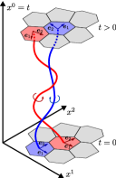
Figure 1: A pictorial illustration of the material triad evolution and continuum particle (finite volumes) rearrangement. The red and blue particles change their neighbors which results in the incompatibility of the local deformation of particles represented by the material basis triads (only $\bm{e}_{1}$ and $\bm{e}_{2}$ are depicted). Initially holonomic $\bm{e}_{1}$, $\bm{e}_{2}$ become non-holonomic at later times.

IV.1 Distortion field

In order to overcome these contradictions and, at the same time, to retain the variational structure of the equations of motion (60), (79) compatible with GR, we follow Godunov and Romenski Godunov and Romenskii (1972); Godunov (1978); Godunov and Romenskii (2003) (and our Newtonian papers Peshkov and Romenski (2016); Dumbser et al. (2016); Peshkov et al. (2017, 2018)) and introduce two deformation fields one of which describes the observable macroscopic deformation while the other describes the internal (non observable for a macroscopic observer) deformation, it is called effective deformation in Godunov and Romenskii (1972); Godunov (1978); Godunov and Romenskii (2003). As the first field, we keep the configuration gradient $\xi^{a}_{\phantom{a}\mu}$ which is integrable or holonomic, i.e. $\partial_{\mu}\xi^{a}_{\phantom{a}\nu}-\partial_{\nu}\xi^{a}_{\phantom{a}\mu}=0$, due to its definition. But this field will play no role in our theory any further. The second deformation field, denoted as $A^{m}_{\ \,\mu}$, is called the 4-distortion and defined as the solution to the following evolution equation (coupled with the energy-momentum conservation which will be discussed later)

$$u^{\nu}\nabla_{\nu}A^{m}_{\ \,\mu}+A^{m}_{\ \,\nu}\nabla_{\mu}u^{\nu}=S^{m}_{\ \mu},\quad\text{or}\quad\mathcal{L}_{\bm{u}}A^{m}_{\ \,\mu}=S^{m}_{\ \mu},$$ (80)

which are different from the evolution of the configuration gradient (77) by the presence of algebraic source term $S^{m}_{\ \mu}(A^{a}_{\ \,\mu})$ which acts as the source of anholonomy.

In order to emphasize that, in general, the stress-free matter configuration corresponding to the distortion field $A^{m}_{\ \,\mu}$ might be different from the initial stress-free configuration corresponding to $\xi^{a}_{\phantom{a}\mu}$ and labeled with $\xi^{a}$, from now on, we shall use middle Latin alphabet letters $m,n,l=0,1,2,3$ and ${M},{N},{L}=1,2,3$ to denote matter-time components, $A^{m}_{\ \,\mu}$, and pure matter components, $A^{{M}}_{\ \,\mu}$, of the distortion field.

Because the mapping $x^{\mu}(\xi^{a})$ may not exist in general, the definition of the 4-velocity (21) cannot be used. Nevertheless, as previously in (28), we still can define the 4-velocity as the 1-st column of the inverse distortion $A^{\mu}_{\ a}$ ($A^{\mu}_{\ a}A^{a}_{\ \,\nu}=\delta^{\mu}_{\ \nu}$, $A^{\mu}_{\ a}A^{b}_{\ \,\mu}=\delta^{b}_{\ a}$), e.g. see Peshkov et al. (2019a),

$$u^{\mu}:=A^{\mu}_{\ 0}.$$ (81)

In particular,

$$A^{0}_{\ \,\mu}u^{\mu}=1,\qquad A^{{M}}_{\ \,\mu}u^{\mu}=0.$$ (82)

Furthermore, we define the source of non-holonomy $S^{m}_{\ \mu}$ satisfying the following four properties

invertibility: $$\quad\det(A^{m}_{\ \,\mu})>0,$$ (83a)

orthogonality: $$\quad A^{{M}}_{\ \,\mu}u^{\mu}=0,$$ (83b)

non-integrability: $$\quad T^{m}_{\ \mu\nu}:=\partial_{\mu}A^{m}_{\ \,\nu}-\partial_{\nu}A^{m}_{\ \,\mu}\neq 0,$$ (83c)

irreversibility: $$\quad\nabla_{\mu}(su^{\mu})\geq 0.$$ (83d)

Here, $s$ is the entropy density, $T^{m}_{\ \mu\nu}$ is the torsion tensor Peshkov et al. (2019a) and, in general, is not assumed to be equal to zero. In other words, the condition (83c) is the mathematical expression of the microscopic structural rearrangements which imply that if a 4-potential, say $A^{m}(x^{\mu})$, would exist it would be a discontinuous (a closed loop on the material manifold becomes open during the evolution) because the connectivity between microscopic parts of the media may not be preserved in the irreversible deformations. The torsion tensor $T^{m}_{\ \mu\nu}$ thus represents a continuous distribution of the density of such microscopic discontinuities, e.g. see Peshkov et al. (2019a); Kleinert (2008) and references therein.

IV.1.1 Local relaxed reference frame

Because a global coordinate system $A^{m}(x^{\mu})$ such that $\partial_{\mu}A^{m}=A^{m}_{\ \,\mu}$ does not exist in general due to the non-integrability condition (83c), one therefore needs to define what is meant under unstressed reference frame in the context of irreversible deformations. In the absence of the global coordinate system, a reference frame can be defined locally for each material element individually. Actually, this is the distortion field itself who introduces the local reference frame. Indeed, due to the invertability condition (83a), the inverse distortion $A^{\mu}_{\ n}$ exists and represents a basis tetrad. Such a tetrad, if pulled-back by the distortion $A^{m}_{\ \,\mu}A^{\mu}_{\ \,n}=\delta^{m}_{\ \,n}$, becomes the orthonormal tetrad $\delta^{m}_{\ \,n}$. The orthonormal tetrad $\delta^{m}_{\ \,n}$ represents the local reference frame with respect to which one can measure the deformation of the given material element. The locality means that in different material elements, the spatial directions (triad) of such an orthonormal tetrad may differ by an arbitrary spatial rotation, while the time direction is implied to be the same for all the material elements and be oriented in the direction of the proper time, see (83b). Furthermore, the local reference frame is also identified with the new relaxed or stress-free state of a given material element. In other words, if the tetrad $A^{\mu}_{\ n}$ and $\delta^{m}_{\ n}$ differ by only a spatial rotation $R^{m}_{\ \mu}$, that is $R^{m}_{\ \mu}A^{\mu}_{\ n}=\delta^{m}_{\ n}$, we say that the material element is locally relaxed.

The key difference between $A^{m}_{\ \,\mu}$ and $\xi^{a}_{\phantom{a}\mu}$ is that the stress-free state associated with $\xi^{a}_{\phantom{a}\mu}$ can be reached globally for all the material elements simultaneously, while the local stress-free states associated with the distortion field $A^{m}_{\ \,\mu}$ cannot be reached simultaneously because there is no such a continuous motion $A^{m}(x^{\mu})$ which could map all the material elements from their current deformed state to the stress-free state.

IV.1.2 Strain measure

Because the stresses in the irreversibly deforming matter depend not on the observable deformation encoded in $\xi^{a}_{\phantom{a}\mu}$, but on the deviation from the local stress-free state encoded now in $A^{m}_{\ \,\mu}$, the spatial metric $\mathcal{G}_{\mu\nu}=\mathcal{G}_{ab}\xi^{a}_{\phantom{a}\mu}\xi^{b}_{\phantom{b}\nu}$ cannot be used to measure material distances anymore. Therefore, it is implied that, in the local reference frame given by $A^{m}_{\ \,\mu}$, the mater-time element is characterized with the axiomatically given metric $\kappa_{mn}$ which, in the absence of phase transformations and other physicochemical changes at the molecular level, is assumed to be locally identical to ${\kappa_{ab}}$ from Section III.2, i.e. it is assumed to be locally flat $\kappa_{mn}=\text{diag}(-1,1,1,1)$. Furthermore, we introduce a new material metric (it is called the effective metric tensor in Godunov (1972); Godunov and Romenskii (2003) in the non-relativistic context),

$$G_{\mu\nu}:=G_{mn}A^{m}_{\ \,\mu}A^{n}_{\ \,\nu}=\kappa_{{M}{N}}A^{M}_{\ \,\mu}A^{N}_{\ \,\nu},$$ (84)

where, similar to (30), we have defined the matter projector in the local relaxed frame

$$G_{mn}:={\kappa_{mn}}+U_{m}U_{n}=\left(\begin{array}[]{rccc}0&0&0&0\\ 0&&&\\ 0&&\kappa_{{M}{N}}&\\ 0&&&\end{array}\right).$$ (85)

As in (30), $U_{m}=(-1,0,0,0)$ because the introduction of the local reference frame concerns only the spatial directions, while it keeps the proper time direction unaffected. Note that if the media is an elastic solid then we have $\xi^{{A}}_{\phantom{{A}}\mu}=A^{{A}}_{\ \,\mu}$ and $\mathcal{G}_{\mu\nu}=G_{\mu\nu}$. Moreover, due to the orthogonality property (83b) of the distortion field, we also have

$$G_{\mu\nu}u^{\mu}=0.$$ (86)

Also, we shall need the contravariant components of the matter projector

$$G^{mn}={\kappa^{mn}}+U^{m}U^{n},\quad G^{\mu\nu}=G^{mn}A^{\mu}_{\ m}A^{\nu}_{\ n}.$$ (87)

IV.1.3 Canonical structure of the energy-momentum tensor

We have defined two deformation fields, one of which, the configuration gradient $\xi^{a}_{\phantom{a}\mu}$, is global and describes the observable deformation of the medium but it says nothing about the changes in the internal structure. The second deformation field, the distortion field $A^{m}_{\ \,\mu}$, is local and characterizes only deformations and rotations of the material elements, while the global deformation of the continuum cannot be recovered from $A^{m}_{\ \,\mu}$. This, however, rises the following issue. The variational principle suggests that the energy-momentum tensor-density $\mathcal{T}^{\nu}_{\ \,\mu}=-(\xi^{a}_{\phantom{a}\mu}\mathcal{E}_{\xi^{a}_{\phantom{a}\nu}}-\delta^{\nu}_{\ \mu}\mathcal{E})$ introduced in (54) is completely specified by defining the energy potential $E(\xi^{a}_{\phantom{a}\mu})$, which, in turn, implies that $\xi^{a}_{\phantom{a}\mu}$ should be treated as a state variable. However, as we just discussed, $\xi^{a}_{\phantom{a}\mu}$ is not related to the internal structure and hence, to the stress state of the media in the case of irreversible deformations (in the elastic case $\xi^{{A}}_{\phantom{{A}}\mu}$ and $A^{{M}}_{\ \,\mu}$ coincide), while the distortion field does characterize the real deformation of the material elements and should play the role of the state variable. In fact, the Euler-Lagrange structure of the energy-momentum tensor-density allows to overcome this contradiction. Indeed, because any two invertible matrices can be related to each other as

$$\xi^{a}_{\phantom{a}\mu}=P^{a}_{\ m}A^{m}_{\ \,\mu},$$ (88)

for some non-degenerate matrix $P^{a}_{\ m}$, and since we assume that the stress state can depend only on actual distances between molecules, the energy may depend on the configuration gradient only via its dependence on the distortion field $A^{m}_{\ \,\mu}$ which dose describe the distances between molecules, see (84), i.e.

$$\mathcal{E}(\xi^{a}_{\phantom{a}\mu})=\hat{\mathcal{E}}(P^{m}_{\ a}\xi^{a}_{\phantom{a}\mu})=\hat{\mathcal{E}}(A^{m}_{\ \,\mu}),$$ (89)

where $P^{m}_{\ \,a}$ is the inverse of $P^{a}_{\ m}$. Therefore, applying the chain rule exactly as in (72), (73), we arrive at

$$-\mathcal{T}^{\nu}_{\ \,\mu}=\xi^{a}_{\phantom{a}\mu}\mathcal{E}_{\xi^{a}_{\phantom{a}\nu}}-\delta^{\nu}_{\ \mu}\mathcal{E}=A^{m}_{\ \,\mu}\hat{\mathcal{E}}_{A^{m}_{\ \,\nu}}-\delta^{\nu}_{\ \mu}\hat{\mathcal{E}},$$ (90)

that is the canonical structure of the energy-momentum is preserved. In the rest of the paper, we remove the “hat” in (89) and write $\mathcal{E}(A^{m}_{\ \,\mu})$.

IV.2 Governing equations

Eventually, we can write down the system of governing equations

$$\nabla_{\mu}\left(A^{m}_{\ \,\nu}\mathcal{E}_{A^{m}_{\ \,\mu}}-\delta^{\mu}_{\ \nu}\mathcal{E}\right)=0,$$ (91a)

$$u^{\nu}\nabla_{\nu}A^{m}_{\ \,\mu}+A^{m}_{\ \,\nu}\nabla_{\mu}u^{\nu}=-\frac{1}{\theta(\tau)}G^{mn}g_{\mu\nu}\mathcal{E}_{A^{n}_{\ \,\nu}},$$ (91b)

$$\nabla_{\mu}(\rho u^{\mu})=0,$$ (91c)

$$\nabla_{\mu}(su^{\mu})=\frac{1}{\mathcal{E}_{s}\theta(\tau)}G^{mn}g_{\mu\nu}\mathcal{E}_{A^{m}_{\ \,\mu}}\mathcal{E}_{A^{n}_{\ \,\nu}}\geq 0,$$ (91d)

which should be closed by providing appropriate functions $\mathcal{E}(A^{{M}}_{\ \,\mu},s)$ and $\theta(\tau)$ where, from now on, $\tau$ stands for the characteristic strain dissipation (or stress relaxation) time but not for the proper time. They will be specified in Sec. IV.4. Also, here, $\mathcal{E}_{s}=\partial\mathcal{E}/\partial s$ stands for the temperature.

The source of non-holonomy $S^{m}_{\ \mu}=-G^{mn}g_{\mu\nu}\mathcal{E}_{A^{n}_{\ \,\nu}}/\theta(\tau)$, as it is defined in (91b), satisfies the four properties (83). In particular, the entropy source term is obviously positive. It is constructed based on the SHTC principle discussed in Sec. II, that is the over-determined system (91) has to be compatible, see details in Sec. IV.7.

The orthogonality condition (83b), is automatically satisfied due the definition of the 4-velocity (81). Nevertheless, in Appendix B, we show that the orthogonality condition (83b) is fulfilled as long as $\mathcal{E}_{A^{{M}}_{\ \,\mu}}u_{\mu}=0$ (which is the case in this paper, see Section IV.3), i.e. the relaxation of the time components $A^{{M}}_{\ \,0}$ is just a consequence of the 4-dimensional formalism.

The non-integrability condition (83c) is also automatically fulfilled for any non-zero source $S^{m}_{\ \mu}$, and the torsion is non-zero in general, e.g. see Peshkov et al. (2019a).

Finally, we have to show that our choice for the source $S^{m}_{\ \mu}$ does not violate the invertibility property (83a). Moreover, as was mentioned in Section III.4.1, we have to show that for the non-holonomic case, i.e. when $\partial_{\nu}A^{m}_{\ \,\mu}-\partial_{\mu}A^{m}_{\ \,\nu}\neq 0$, the rest mass density conservation law (91c) can be derived from the distortion evolution equation (91b). In fact, in order to satisfy our needs, it is sufficient to initiate the distortion field with the condition

$$\det(A^{m}_{\ \,\mu})=\det(\xi^{a}_{\phantom{a}\mu})=\frac{\rho}{\rho_{0}}\sqrt{-g}.$$ (92)

Indeed, in this case, by multiplying (91b) by $\rho_{A^{m}_{\ \,\mu}}=\partial\rho/\partial A^{m}_{\ \,\mu}=\rho A^{\mu}_{\ m}$, one obtains

$$\rho_{A^{m}_{\ \,\mu}}\left(u^{\nu}\nabla_{\nu}A^{m}_{\ \,\mu}+A^{m}_{\ \,\nu}\nabla_{\mu}u^{\nu}\right)=u^{\mu}\nabla_{\mu}\rho+\rho A^{\nu}_{\ m}A^{m}_{\ \,\mu}\nabla_{\nu}u^{\mu}=\nabla_{\mu}(\rho u^{\mu})$$ (93)

for the left hand-side of (91b). Therefore, it remains to show that

$$\rho_{A^{m}_{\ \,\mu}}G^{mn}g_{\mu\nu}\mathcal{E}_{A^{n}_{\ \,\nu}}=\rho_{A^{{M}}_{\ \,\mu}}\kappa^{{M}{N}}g_{\mu\nu}\mathcal{E}_{A^{{N}}_{\ \,\nu}}=0.$$ (94)

This, however, cannot be proved in the general case but is conditioned by the choice of the energy $\mathcal{E}$. Thus, we prove in Section IV.4 (see equation (IV.4)) that for our particular choice of the equation of state, condition (94) is satisfied.

IV.3 Conventional structure of the energy-momentum tensor

Because the energy potential $\mathcal{E}$ is supposed to transform as a scalar-density under transformations of both the spacetime and matter, it may depend on $A^{m}_{\ \,\mu}$ only via the scalars that can be made from $G_{\mu\nu}={\kappa_{{M}{N}}}A^{{M}}_{\ \,\mu}A^{{N}}_{\ \,\nu}$. Also, because $G_{\mu\nu}$ has one zero eigenvalue, there are only three independent scalar invariants. For example,

$$I_{1}=g^{\mu\lambda}G_{\lambda\mu}=G^{\mu}_{\ \mu},\quad I_{2}=G^{\mu}_{\ \nu}G^{\nu}_{\ \mu},\quad I_{3}=G^{\mu}_{\ \nu}G^{\nu}_{\ \lambda}G^{\lambda}_{\ \mu}.$$ (95)

However, it is convenient to replace the third invariant with the rest matter density $\rho$. Indeed, as discussed in Karlovini and Samuelsson (2003); Gundlach et al. (2012), the spacetime tensor $G^{\mu}_{\ \nu}=g^{\mu\lambda}G_{\lambda\nu}$ has the same eigenvalues as the pure matter tensor $G^{{M}}_{\ {N}}:=g^{\mu\nu}\kappa_{{N}{L}}A^{{M}}_{\ \,\mu}A^{{L}}_{\ \,\nu}$ in addition to one zero eigenvalue. Furthermore, in Gundlach et al. (2012), it is also shown that the determinant $\det(G^{{M}}_{\ {N}})$ relates to the rest matter density as $\det(G^{{M}}_{\ {N}})=\rho^{2}$. Therefore, we assume that

$$\mathcal{E}(A^{m}_{\ \,\mu},s)=\mathcal{E}(I_{1},I_{2},\rho,s),$$ (96)

where we also consider a dependence on the entropy density $s=\rho S$ with $S$ being the specific entropy in the rest frame. We are now ready to unveil the conventional structure of the energy-momentum tensor $\mathcal{T}^{\nu}_{\ \,\mu}=-(A^{m}_{\ \,\mu}\mathcal{E}_{A^{m}_{\ \,\nu}}-\delta^{\nu}_{\ \mu}\mathcal{E})$ of our theory. Thus, because of (96), one can write $A^{m}_{\ \,\mu}\mathcal{E}_{A^{m}_{\ \,\nu}}=A^{{M}}_{\ \,\mu}\mathcal{E}_{A^{{M}}_{\ \,\nu}}$. Then, using that $\rho=\frac{1}{\sqrt{-g}}\sqrt{-J^{\mu}J_{\mu}}$, $u^{\mu}=A^{\mu}_{\ 0}$ and the identity (see Kijowski et al. (1990))

$$\frac{\partial J^{\lambda}}{\partial A^{{M}}_{\ \,\nu}}A^{{M}}_{\ \,\mu}=J^{\lambda}\delta^{\nu}_{\ \mu}-J^{\nu}\delta^{\lambda}_{\ \mu},$$ (97)

we may write

$$-\mathcal{T}^{\nu}_{\ \,\mu}=A^{{M}}_{\ \,\mu}\left(\mathcal{E}_{\rho}\frac{\partial\rho}{\partial J^{\lambda}}\frac{\partial J^{\lambda}}{\partial A^{{M}}_{\ \,\nu}}+\mathcal{E}_{A^{{M}}_{\ \,\nu}}\right)-\mathcal{E}\delta^{\nu}_{\ \mu} =$$

$$-\frac{1}{\sqrt{-g}}(\mathcal{E}_{\rho}+S\mathcal{E}_{s})u_{\lambda}(J^{\lambda}\delta^{\nu}_{\ \mu}-J^{\nu}\delta^{\lambda}_{\ \mu})+A^{{M}}_{\ \,\mu}\mathcal{E}_{A^{{M}}_{\ \,\nu}}-\mathcal{E}\delta^{\nu}_{\ \mu} =$$

$$(\rho\mathcal{E}_{\rho}+s\mathcal{E}_{s})(\delta^{\nu}_{\ \mu}+u^{\nu}u_{\mu})+A^{{M}}_{\ \,\mu}\mathcal{E}_{A^{{M}}_{\ \,\nu}}-\mathcal{E}\delta^{\nu}_{\ \mu},$$ (98)

which now can be rewritten in the conventional form

$$-\mathcal{T}^{\nu}_{\ \,\mu}=\mathcal{E}u^{\nu}u_{\mu}+ph^{\nu}_{\ \mu}+\sigma^{\nu}_{\ \mu},$$ (99)

where one can identify the pressure $p$ and the anisotropic part $\sigma^{\nu}_{\ \mu}$ of the energy-momentum tensor as

$$p:=\rho\mathcal{E}_{\rho}+s\mathcal{E}_{s}-\mathcal{E},\qquad\sigma^{\nu}_{\ \mu}:=A^{{M}}_{\ \,\mu}\mathcal{E}_{A^{{M}}_{\ \,\nu}}.$$ (100)

It is necessary to emphasize that while computing $\sigma^{\nu}_{\ \mu}$, the rest mass density $\rho$ and the distortion $A^{{M}}_{\ \,\mu}$ should be treated as independent variables because their dependence has been already taken into account in the pressure. More explicitly, $\sigma^{\nu}_{\ \mu}=A^{{M}}_{\ \,\mu}\left(\frac{\partial\mathcal{E}}{\partial I_{1}}\frac{\partial I_{1}}{\partial A^{{M}}_{\ \,\nu}}+\frac{\partial\mathcal{E}}{\partial I_{2}}\frac{\partial I_{2}}{\partial A^{{M}}_{\ \,\nu}}\right)$.

Finally, we note that due to the orthogonality condition $A^{{M}}_{\ \,\mu}u^{\mu}=0$, the following orthogonality conditions are hold for the anisotropic part of the energy-momentum

$$\sigma^{\nu}_{\phantom{\nu}\mu}u^{\mu}=0,\qquad\sigma^{\nu}_{\phantom{\nu}\mu}u_{\nu}=0.$$ (101)

While (101)₁ is obvious, (101)₂ follows from (96) and the formulas

$$\frac{\partial I_{1}}{\partial A^{{M}}_{\ \,\mu}}=2\,\kappa_{{M}{N}}A^{{N}}_{\ \,\lambda}{g^{\lambda\mu}}=2\,\kappa_{{M}{N}}A^{{N}}_{\ \,\lambda}{h^{\lambda\mu}},\quad\frac{\partial I_{2}}{\partial A^{{M}}_{\ \,\mu}}=4\,\kappa_{{M}{N}}A^{{N}}_{\ \,\lambda}G^{\lambda}_{\ \nu}{g^{\nu\mu}}=4\,\kappa_{{M}{N}}A^{{N}}_{\ \,\lambda}G^{\lambda}_{\ \nu}{h^{\nu\mu}}.$$ (102)

These derivatives are obviously orthogonal to $u_{\mu}$.

IV.4 Equation of state

In this section, we give a particular expression to the specific energy

$$1+\varepsilon(I_{1},I_{2},\rho,S):=\rho^{-1}\mathcal{E}(I_{1},I_{2},\rho,s).$$ (103)

Following our papers on Newtonian continuum mechanics Dumbser et al. (2016, 2017), we shall decompose tensor $G_{\mu\nu}$ on the traceless, $\mathring{G}_{\mu\nu}$, and spherical parts

$$G_{\mu\nu}=\mathring{G}_{\mu\nu}+\frac{G^{\lambda}_{\ \lambda}}{3}h_{\mu\nu},\quad\text{ where }\quad\mathring{G}_{\mu\nu}:=G_{\mu\nu}-\frac{G^{\lambda}_{\ \lambda}}{3}h_{\mu\nu}.$$ (104)

Note that, in this definition, $\mathring{G}_{\mu\nu}$ refers to $h_{\mu\nu}$ and not to the full spacetime metric $g_{\mu\nu}$. We then use the norm of the traceless part (here one has to use $h^{\mu}_{\ \mu}=g^{\mu\lambda}h_{\lambda\mu}=3$)

$$\mathring{G}^{\lambda}_{\ \nu}\mathring{G}^{\nu}_{\ \lambda}=I_{2}-I_{1}^{2}/3,$$ (105)

as an indication of the presence of non-volumetric deformations, and define the specific energy $\varepsilon(I_{1},I_{2},\rho,S)$ as

$$\varepsilon(I_{1},I_{2},\rho,S)=\varepsilon^{\rm eq}(\rho,S)+\frac{c_{s}^{2}}{4}\mathring{G}^{\lambda}_{\ \nu}\mathring{G}^{\nu}_{\ \lambda}$$ (106)

where $\varepsilon^{\rm eq}$ is the internal (equilibrium) part of the total energy, and $c_{s}$ is the sound speed for the shear perturbation propagation. This sound speed may depend on $\rho$ and $S$ but we do not consider this possibility in this paper. The non-equilibrium term (the second term on the right hand-side of (106)) is due to the distortion of the material elements. Such a simple equation of state serves only as an example which nevertheless allows us to demonstrate all of the important features of our unified framework including dynamics of solids and fluids. It is also important to emphasize that the shear momentum transfer (as well as other transfer processes) occurs in an intrinsically transient way in the SHTC framework in contrast to the steady-state classical transport theory based on the viscosity concept and the steady-state Newton’s viscous law. The transient character of our theory is expressed in that the transport coefficient are the velocity and time characteristics, $c_{s}$ and $\tau$, accordingly. Such characteristics can be recovered only from transient experiments such as high frequency sound wave propagation, see Dumbser et al. (2016); Peshkov et al. (2017). We thus stress that the classical steady-state viscosity concept is not used in our theory either explicitly nor implicitly.

When we shall deal with gases in the numerical examples we shall use the ideal gas equation of state for the equilibrium part $\varepsilon^{\rm eq}$ of the energy

$$\varepsilon^{\rm eq}(\rho,S)=\frac{c^{2}_{0}}{\gamma(\gamma-1)},\quad c_{0}^{2}=\gamma\rho^{\gamma-1}e^{S/c_{V}},$$ (107a)

or the so-called stiffened gas equation of state

$$\varepsilon^{\rm eq}(\rho,S)=\dfrac{c^{2}_{0}}{\gamma(\gamma-1)}\left(\dfrac{\rho}{\rho_{0}}\right)^{\gamma-1}e^{S/c_{V}}+\dfrac{\rho_{0}c_{0}^{2}-\gamma p_{0}}{\gamma\rho},\quad c_{0}^{2}=const,$$ (107b)

if we want to deal with liquids or solids. In both cases, $c_{0}$ has the meaning of the adiabatic sound speed, $c_{V}$ is the specific heat capacity at constant volume, $\gamma$ is the ratio of the specific heats, i.e. $\gamma=c_{p}/c_{V}$, if $c_{p}$ is the specific heat capacity at constant pressure. In (107b), $\rho_{0}$ is the reference mass density, $p_{0}$ is the reference (atmospheric) pressure.

Giving an equation of state for $\mathcal{E}$ closes the model formulation. Thus, we now may compute the anisotropic part $\sigma^{\nu}_{\ \mu}$ of the energy-momentum tensor and the dissipative source term in the evolution equation (91b) for the distortion field. Differentiating of $\mathcal{E}$ with respect to $A^{{M}}_{\ \,\mu}$ gives the formula similar to its Newtonian analog (see equation (9) in Dumbser et al. (2016))

$$\mathcal{E}_{A^{{M}}_{\ \,\mu}}=\rho\,c_{s}^{2}\kappa_{{M}{N}}A^{{N}}_{\ \,\lambda}g^{\lambda\alpha}\mathring{G}_{\alpha\beta}h^{\beta\mu},$$ (108)

where we have used formulas (102).

Furthermore, it is now clear how to choose function $\theta(\tau)$ in (91b) to make the physical units on the right and left-hand side of (91b) agree, e.g. $\theta(\tau)\sim\rho\,\tau c_{s}^{2}$. We choose

$$\theta(\tau)=\rho_{0}\,\tau c_{s}^{2}G^{\lambda}_{\ \lambda}/3.$$ (109)

The trace $G^{\lambda}_{\ \lambda}/3$ appears here for convenience only which later makes it easier the computation of the effective viscosity of our model.

Eventually, formula (100) for the covariant component of the stress tensor-density $\sigma_{\mu\nu}$ can be written explicitly (recall that we treat $\rho$ and $A^{{M}}_{\ \,\mu}$ as independent variables in (100))

$$\sigma_{\mu\nu}=g_{\mu\lambda}\sigma^{\lambda}_{\phantom{\lambda}\nu}=\,g_{\mu\lambda}A^{{M}}_{\ \,\nu}\mathcal{E}_{A^{{M}}_{\ \,\lambda}}=\rho\,c_{s}^{2}\mathring{G}_{\mu\lambda}G^{\lambda}_{\ \nu}.$$ (110)

Also, note that if one wants to incorporate the volume relaxation (volume viscosity) effect one just need to add an extra non-equilibrium term in the energy potential:

$$\varepsilon(A^{{M}}_{\ \,\mu},\rho,S)=\varepsilon^{\rm eq}(\rho,S)+\frac{c_{s}^{2}}{4}\mathring{G}^{\lambda}_{\ \nu}\mathring{G}^{\nu}_{\ \lambda}+\frac{c_{v}^{2}}{2}\left(\frac{w}{\sqrt{-g}}-\frac{\rho}{\rho_{0}}\right)^{2},$$ (111)

where $c_{v}$ is a velocity that will contribute to the sound speed of propagation of volume perturbations at high frequencies, $w=\det(A^{m}_{\ \,\mu})$, see (92). This extra term, of course, affects the computation of (108) and (110). An effective volume viscosity then can be identified as $\sim\tau(c_{0}^{2}+c_{v}^{2})$ in the same way as we identify the effective shear viscosity, see details in Sec. IV.5. Here, $c_{0}$ is the adiabatic (low frequency) sound speed from (107).

Finally, we have to prove that our choice of the energy potential is consistent with the rest mass density conservation law, i.e. that the condition (94) is fulfilled. Indeed, one has (without losing the generality, we shall omit $\rho c_{s}^{2}>0$ factor in $\mathcal{E}_{A^{{N}}_{\ \,\nu}}$):

$$\rho_{A^{{M}}_{\ \,\mu}}\kappa^{{M}{N}}g_{\mu\nu}\mathcal{E}_{A^{{N}}_{\ \,\nu}}=\rho A^{\mu}_{\ {M}}\kappa^{{M}{N}}g_{\mu\nu}\mathcal{E}_{A^{{N}}_{\ \,\nu}} =$$

$$\rho A^{\mu}_{\ {M}}\kappa^{{M}{N}}g_{\mu\nu}\kappa_{{N}{K}}A^{{K}}_{\ \,\lambda}g^{\lambda\alpha}\mathring{G}_{\alpha\beta}h^{\beta\nu} =$$

$$\rho\mathring{G}_{\alpha\beta}h^{\beta\alpha}=\rho h^{\beta\alpha}\left(G_{\alpha\beta}-\frac{I_{1}}{3}h_{\alpha\beta}\right) =$$

$$\rho\left(I_{1}-\frac{I_{1}}{3}h^{\beta\alpha}h_{\alpha\beta}\right) =0.$$ (112)

IV.5 Asymptotic analysis in the diffusive regime

As we discussed in the previous section, our theory does not rely on the classical steady-state viscosity approach, but nevertheless, we may perform a formal asymptotic analysis for $\tau\rightarrow 0$ (i.e. we are in the diffusive regime) and show that, in the leading terms, the viscous stress is similar to the relativistic Navier-Stokes stress obtained by Landau and Lifshitz Landau and Lifshitz (2004) and thus we may obtain an expression for the effective viscosity coefficient in terms of transient characteristics $c_{s}$ and $\tau$. However, it is necessary to recall that the relativistic Navier-Stokes stress leads to the acausal governing PDEs, e.g. Muller and Ruggeri (1998); Rezzolla and Zanotti (2013), which results also in the numerical instabilities. Because our model is hyperbolic and hence causal, it is thus clear that this is the high order terms in $\tau$ of the model who damp the unstable modes in the relativistic Navier-Stokes equations.

In this section, it is convenient to use the evolution equation for the effective metric tensor $G_{\mu\nu}$ since the stress $\sigma_{\mu\nu}$ depends on $A^{{M}}_{\ \,\mu}$ only through $G_{\mu\nu}$. The evolution of $G_{\mu\nu}$ reads as

$$u^{\lambda}\nabla_{\lambda}G_{\mu\nu}+G_{\mu\lambda}\nabla_{\nu}u^{\lambda}+G_{\lambda\nu}\nabla_{\mu}u^{\lambda}=-\frac{2}{\tau\,\vartheta}\sigma_{\mu\nu},$$ (113)

where $\vartheta=\theta/\tau=\rho_{0}\,c_{s}^{2}G^{\lambda}_{\ \lambda}/3$. This PDE is the direct consequence of the distortion evolution (91b), the advection equation for $\kappa^{{M}{N}}$, $u^{\lambda}\nabla_{\lambda}\kappa^{{M}{N}}=0,$ and the identity

$${\rm d}G_{\mu\nu}=A^{{M}}_{\ \,\mu}\kappa^{{M}{N}}({\rm d}A^{{N}}_{\ \,\nu})+A^{{M}}_{\ \,\mu}({\rm d}\kappa^{{M}{N}})A^{{N}}_{\ \,\nu}+({\rm d}A^{{M}}_{\ \,\mu})\kappa^{{M}{N}}A^{{N}}_{\ \,\nu}.$$ (114)

After taking the traceless part of the covariant PDE for $G_{\mu\nu}$ (113) and replacing $G_{\lambda\beta}$ by $\mathring{G}_{\lambda\beta}+\frac{1}{3}G^{\lambda}_{\ \lambda}h_{\lambda\beta}(=G_{\lambda\beta})$, we have the following PDE

$$u^{\lambda}\nabla_{\lambda}\mathring{G}_{\mu\nu}+\mathring{G}_{\mu\lambda}\nabla_{\nu}u^{\lambda}+\mathring{G}_{\lambda\nu}\nabla_{\mu}u^{\lambda}+2GD_{\mu\nu}-\frac{2}{3}\left(h^{\alpha\beta}G_{\lambda\beta}\nabla_{\alpha}u^{\lambda}\right)h_{\mu\nu}+{Gu^{\lambda}\nabla_{\lambda}h_{\mu\nu}}=-\frac{2}{\tau\,\vartheta}\mathring{\sigma}_{\mu\nu},$$ (115)

where

$$D_{\mu\nu} :=\frac{1}{2}\left(h_{\mu\lambda}\nabla_{\nu}u^{\lambda}+h_{\lambda\nu}\nabla_{\mu}u^{\lambda}\right),$$ (116a)

$$\mathring{\sigma}_{\mu\nu} :=\sigma_{\mu\nu}-\frac{\sigma^{\lambda}_{\ \lambda}}{3}h_{\mu\nu},\qquad G:=\frac{1}{3}G^{\lambda}_{\ \lambda}$$ (116b)

are the symmetric 4-velocity gradient, the trace-less part of the stress tensor, and one-third of the trace of $G_{\mu\nu}$, accordingly.

After once more replacing $G_{\lambda\beta}$ by $\mathring{G}_{\lambda\beta}+Gh_{\lambda\beta}$ we arrive at the final PDE for the trace-less part $\mathring{G}_{\mu\nu}$

$$u^{\lambda}\nabla_{\lambda}\mathring{G}_{\mu\nu}+\mathring{G}_{\mu\lambda}\nabla_{\nu}u^{\lambda}+\mathring{G}_{\lambda\nu}\nabla_{\mu}u^{\lambda}+2G\mathring{D}_{\mu\nu}-\frac{2}{3}\left(h^{\alpha\beta}\mathring{G}_{\lambda\beta}\nabla_{\alpha}u^{\lambda}\right)h_{\mu\nu}+{Gu^{\lambda}\nabla_{\lambda}h_{\mu\nu}}=-\frac{2}{\tau\,\vartheta}\mathring{\sigma}_{\mu\nu},$$ (117)

where $\mathring{D}_{\mu\nu}=D_{\mu\nu}-(D^{\lambda}_{\ \lambda}/3)h_{\mu\nu}$ is the trace-less part of the symmetric velocity gradient $D_{\mu\nu}$. We now assume that the solution to (117) can be written as

$$\mathring{G}_{\mu\nu} =\mathring{G}_{\mu\nu}^{(0)}+\tau\mathring{G}_{\mu\nu}^{(1)}+\tau^{2}\mathring{G}_{\mu\nu}^{(2)}+\ldots\,,$$ (118a)

$$\rho =\rho_{0}+\tau\rho_{1}+\tau^{2}\rho_{2}+\ldots\,,$$ (118b)

$$G =G^{(0)}+\tau G^{(1)}+\tau^{2}G^{(2)}+\ldots\,,$$ (118c)

and will show that the relativistic Euler equations are recovered if only zeroth order terms are retained, and the relativistic Navier-Stokes equations are recovered if the first-order terms in $\tau$ are retained.

Zeroth-order approximation (Euler fluid):

After plugging (118a) into the PDE (117), and collecting leading order terms ($\tau^{0}$), we have that

$$\mathring{G}_{\mu\nu}^{(0)}=0,$$ (119)

and hence

$$G_{\mu\nu}^{(0)}=G^{(0)}h_{\mu\nu}\quad\text{ with }\quad G^{(0)}=\frac{1}{3}g^{\alpha\beta}G_{\beta\alpha}^{(0)}=1,$$ (120)

which results in that $\sigma_{\mu\nu}=0$ and hence, the energy-momentum tensor reduces to the one of the relativistic Euler equations.

First-order approximation (Navier-Stokes):

If we now plug (118a) into the stress tensor $\sigma_{\mu\nu}=\rho\,c_{s}^{2}\mathring{G}_{\mu\lambda}G^{\lambda}_{\ \nu}$ and keep only leading terms of the order $\tau^{1}$, we have

$$\sigma_{\mu\nu}=\,c_{s}^{2}\left((\rho_{0}+\tau\rho_{1})\mathring{G}_{\mu\lambda}^{(0)}G_{\alpha\nu}^{(0)}+\tau\rho_{0}\left(G_{\alpha\nu}^{(1)}\mathring{G}_{\mu\lambda}^{(0)}+\mathring{G}_{\mu\lambda}^{(1)}G_{\alpha\nu}^{(0)}\right)\right)h^{\lambda\alpha}+\ldots$$ (121)

which, because of (119), (120), and the orthogonality condition, simplifies to

$$\sigma_{\mu\nu}=\rho_{0}c_{s}^{2}\tau\mathring{G}_{\mu\lambda}^{(1)}G_{\alpha\nu}^{(0)}h^{\lambda\alpha}=\rho_{0}c_{s}^{2}\tau\mathring{G}_{\mu\lambda}^{(1)}G^{(0)}h^{\lambda}_{\ \nu}=\rho_{0}\tau c_{s}^{2}\mathring{G}_{\mu\lambda}^{(1)}h^{\lambda}_{\ \nu}.$$ (122)

It also follows from this result that $h^{\alpha\beta}\sigma_{\alpha\beta}=0$, i.e. at first order the stress $\sigma_{\mu\nu}$ is trace-less, $\mathring{\sigma}_{\mu\nu}=\sigma_{\mu\nu}$.

From the other hand, if we plug expansion (118a) into the PDE (117), in leading terms, we have

$$2\mathring{D}_{\mu\nu}+{u^{\lambda}\nabla_{\lambda}h_{\mu\nu}}=-\frac{2}{\rho_{0}c_{s}^{2}}\rho_{0}c_{s}^{2}\mathring{G}_{\mu\lambda}^{(1)}h^{\lambda}_{\ \nu}.$$ (123)

Now, using that $\mathring{G}_{\mu\lambda}^{(1)}h^{\lambda}_{\ \nu}=\sigma_{\mu\nu}/(\rho_{0}\tau c_{s}^{2})$, see (122), and the definition of $\mathring{D}_{\mu\nu}$, the last equality transforms into

$$-\frac{1}{\rho_{0}\tau c_{s}^{2}}\sigma_{\mu\nu}=\frac{1}{2}\left(h_{\mu\lambda}\nabla_{\nu}u^{\lambda}+h_{\lambda\nu}\nabla_{\mu}u^{\lambda}-\vphantom{\frac{2}{3}}\frac{2}{3}(h^{\alpha}_{\ \lambda}\nabla_{\alpha}u^{\lambda})h_{\mu\nu}+{u^{\lambda}\nabla_{\lambda}h_{\mu\nu}}\right),$$ (124)

which is equivalent to the Landau-Lifshitz version of the relativistic Navier-Stokes stress Landau and Lifshitz (2004); Rezzolla and Zanotti (2013) (to see this, it is only necessary to take into account that $u_{\lambda}\nabla_{\nu}u^{\lambda}=0$ and $\nabla_{\lambda}g_{\mu\nu}=0$)

$$\tau^{{\rm NS}}_{\mu\nu}:=-\mu\left(\nabla_{\nu}u_{\mu}+\nabla_{\mu}u_{\nu}+u^{\lambda}\nabla_{\lambda}(u_{\mu}u_{\nu})-\vphantom{\frac{2}{3}}\frac{2}{3}(h^{\alpha\lambda}\nabla_{\lambda}u_{\alpha})h_{\mu\nu}\right).$$ (125)

Hence, for small $\tau$, we may identify an effective shear viscosity coefficient for our model:

$$\mu:=\frac{1}{6}\rho_{0}\tau c_{s}^{2}.$$ (126)

3+1 version:

Since, in the numerical simulation, we use the 3+1 split of the spacetime, it is also necessary to know the viscosity in this case. Thus, using that $(\gamma,\gamma\hat{v}^{i})=(u^{0},u^{i})$, $\gamma=\alpha^{-1}W$, where $\alpha$ is the time lapse and $W$ is the Lorentz factor, we can rewrite the stress (124) as

$$-\sigma_{\mu\nu}=\mu\left(h_{\mu 0}\partial_{\nu}\gamma+h_{\mu j}\partial_{\nu}(\gamma\hat{v}^{j})+h_{0\mu}\partial_{\mu}\gamma+\vphantom{\frac{2}{3}}h_{j\nu}\partial_{\mu}(\gamma\hat{v}^{j})-\frac{2}{3}(h^{\alpha}_{\ 0}\partial_{\alpha}\gamma+h^{\alpha}_{\ j}\partial_{\alpha}(\gamma\hat{v}^{j}))h_{\mu\nu}+\vphantom{\frac{2}{3}}\gamma\partial_{0}h_{\mu\nu}+\gamma\hat{v}^{j}\partial_{j}h_{\mu\nu}\right).$$ (127)

Further, using that $h_{\mu\nu}$ is the projector, we may write

$$h_{\mu 0}\partial_{\nu}\gamma+h_{\mu j}\partial_{\nu}(\gamma\hat{v}^{j})=h_{\mu 0}\partial_{\nu}\gamma+h_{\mu j}\hat{v}^{j}\partial_{\nu}\gamma+\gamma h_{\mu j}\partial_{\nu}\hat{v}^{j}=\gamma h_{\mu j}\partial_{\nu}\hat{v}^{j},$$ (128)

and hence

$$-\sigma_{\mu\nu}=\mu\gamma\left(h_{\mu j}\partial_{\nu}\hat{v}^{j}+h_{j\nu}\partial_{\mu}\hat{v}^{j}-\vphantom{\frac{2}{3}}\frac{2}{3}(h_{j}^{\alpha}\partial_{\alpha}\hat{v}^{j})h_{\mu\nu}+\partial_{t}h_{\mu\nu}+\hat{v}^{j}\partial_{j}h_{\mu\nu}\right).$$ (129)

Therefore, if $\mu$ denotes the viscosity coefficient in the covariant version (124) and $\hat{\mu}$ denotes the viscosity coefficient in the 3+1 split then they relate to each other as

$$\hat{\mu}=\gamma\mu,\qquad\gamma=\alpha^{-1}W.$$ (130)

IV.6 Comparison with the Müller-Israel-Stewart model

In this section we compare our equations with the state of the art relativistic dissipative fluid dynamics model, the Israel-Stewart model (also known as Müller-Israel-Stewart model) Mueller (1966); Israel (1976); Stewart (1977), which is actively used in the special relativistic context, and in particular for relativistic heavy-ion collisions, e.g. Del Zanna et al. (2013); Karpenko et al. (2014); Shen et al. (2016). However, since we ignore in this paper the volume relaxation effect and the heat conduction, we shall compare only the PDEs for the evolution of the shear stress tensor. The volume relaxation can be incorporated in the current framework as it is discussed in (111). The hyperbolic heat conduction in the SHTC framework also has a variational nature, e.g. see Peshkov et al. (2018), and can be incorporated in a straightforward manner in the present model. This will be the subject for further publications.

The Israel-Stewart equation for the trace-less shear stress tensor $\tau_{\mu\nu}$ (without the temperature terms) reads as, see e.g. Rezzolla and Zanotti (2013),

$$\lambda\,h^{\alpha}_{\ \mu}h^{\beta}_{\ \nu}\overset{\bm{\cdot}}{\tau}_{\alpha\beta}+\tau_{\mu\nu}=-2\mu\tau^{{\rm NS}}_{\mu\nu},$$ (131)

where

$$\tau^{{\rm NS}}_{\mu\nu}:=\frac{1}{2}\left(L_{\nu\mu}+L_{\mu\nu}+u^{\gamma}\nabla_{\gamma}(u_{\mu}u_{\nu})\right)-\frac{1}{3}(h^{\alpha\gamma}\nabla_{\gamma}u_{\alpha})h_{\mu\nu},$$

is the relativistic Navier-Stokes stress tensor, $\lambda$ is the relaxation time associated with the time scale of the relaxation of the shear stress to its equilibrium value $\tau^{{\rm NS}}_{\mu\nu}$, the overdot symbol stands for the convective derivative $\overset{\bm{\cdot}}{\tau}_{\mu\nu}:=u^{\gamma}\nabla_{\gamma}\tau_{\mu\nu}$, while $L^{\mu}_{\ \nu}=\nabla_{\nu}u^{\mu}$, $L_{\mu\nu}=g_{\mu\gamma}L^{\gamma}_{\ \nu}$ is the velocity gradient tensor. Therefore, it only remains to obtain the evolution equation for the shear stress tensor (110) and to compare it with (131). This is however not a trivial task in the general case even for the simple equation of state (106) due to the nonlinear relation between the distortion field $A^{{M}}_{\ \,\mu}$ and the shear stress $\sigma_{\mu\nu}$. Nevertheless, this can be done relatively easily if to assume the smallness of $\sigma_{\mu\nu}$ in $\mathring{G}_{\mu\nu}$, that is we shall assume the approximation

$$\sigma_{\mu\nu}=\rho\,c_{s}^{2}\mathring{G}_{\mu\lambda}G^{\lambda}_{\ \nu}=\rho\,c_{s}^{2}\mathring{G}_{\mu\lambda}(\mathring{G}^{\lambda}_{\ \nu}+Gh^{\lambda}_{\ \nu})\approx\rho\,c_{s}^{2}\,G\,\mathring{G}_{\mu\nu},\qquad G=\frac{1}{3}G^{\lambda}_{\ \lambda}.$$ (132)

Also, recall that in this paper it is assumed that $c_{s}=const$. We note that, in general, the shear stress $\sigma_{\mu\nu}$ is not necessary trace-less and hence already has some contribution to the bulk viscosity effect but its linear approximation in $\mathring{G}_{\mu\nu}$ (132) has obviously zero trace.

We then apply the convective derivative $u^{\gamma}\nabla_{\gamma}$ to the approximation (132) to obtain

$$\overset{\bm{\cdot}}{\sigma}_{\mu\nu}=\overset{\bm{\cdot}}{\rho}c_{s}^{2}G\mathring{G}_{\mu\nu}+\overset{\bm{\cdot}}{G}\rho c_{s}^{2}\mathring{G}_{\mu\nu}+\overset{\bm{\cdot}}{\mathring{G}}_{\mu\nu}\rho c_{s}^{2}G.$$ (133)

Note that if one wants to obtain the PDE for the full shear stress tensor, (133) should be replaced with

$$\overset{\bm{\cdot}}{\sigma}_{\mu\nu}=\overset{\bm{\cdot}}{\rho}c_{s}^{2}(G\mathring{G}_{\mu\nu}+\mathring{G}_{\mu\lambda}\mathring{G}^{\lambda}_{\ \nu})+\overset{\bm{\cdot}}{G}\rho c_{s}^{2}\mathring{G}_{\mu\nu}+\rho c_{s}^{2}(G\overset{\bm{\cdot}}{\mathring{G}}_{\mu\nu}+\overset{\bm{\cdot}}{\mathring{G}}_{\mu\lambda}\mathring{G}^{\lambda}_{\ \nu})+\rho c_{s}^{2}\mathring{G}_{\mu\lambda}\overset{\bm{\cdot}}{\mathring{G}^{\lambda}_{\ \nu}}.$$ (134)

From the rest mass conservation $\nabla_{\mu}(\rho u^{\mu})=0$ we can obtain that $\overset{\bm{\cdot}}{\rho}=-\rho L^{\lambda}_{\ \lambda}$, while the PDE for $\overset{\bm{\cdot}}{G}$ can be obtained by applying $u^{\gamma}\nabla_{\gamma}$ to (113). Thus, we have

$$\overset{\bm{\cdot}}{G}=-\frac{2}{3}(\mathring{G}^{\nu}_{\ \lambda}+Gh^{\nu}_{\ \lambda})L^{\lambda}_{\ \nu}.$$ (135)

Eventually, the evolution equation for $\overset{\bm{\cdot}}{\mathring{G}}_{\mu\nu}$ is given by (117).

After plugging expressions for $\overset{\bm{\cdot}}{\rho}$, $\overset{\bm{\cdot}}{G}$, and $\overset{\bm{\cdot}}{\mathring{G}}_{\mu\nu}$ into (133) and after a few term rearrangements we arrive at

$$\frac{\tau}{2}\left(\overset{\bm{\cdot}}{\sigma}_{\mu\nu}+\sigma_{\mu\nu}L^{\lambda}_{\ \lambda}+\frac{5}{3}\sigma_{\mu\lambda}L^{\lambda}_{\ \nu}+\sigma_{\lambda\nu}L^{\lambda}_{\ \mu}-\vphantom{\frac{2}{3}}\frac{2}{3}(\sigma^{\alpha}_{\ \lambda}L^{\lambda}_{\ \alpha})h_{\mu\nu}\right)+\sigma_{\mu\nu}=-2\mu\sigma^{{\rm NS}}_{\mu\nu},$$ (136a)

where

$$\sigma^{{\rm NS}}_{\mu\nu}=\frac{1}{2}\left(L_{\mu\nu}+L_{\nu\mu}+u^{\gamma}\nabla_{\gamma}(u_{\mu}u_{\nu})\right)-\frac{1}{3}(h^{\alpha}_{\ \lambda}L^{\lambda}_{\ \alpha})h_{\mu\nu}.$$ (136b)

Thus, we can directly compare equations (131) and (136a). It is obvious that $\tau^{{\rm NS}}_{\mu\nu}$ and $\sigma^{{\rm NS}}_{\mu\nu}$ are identical and the main difference is in the first terms of (131) and (136a). Thus, one may expect that the solutions to the Israel-Stewart theory and our theory are close for the flows not far from the equilibrium, i.e. when the Navier-Stokes terms dominate. The solutions will diverge as long as the flow becomes more and more non-equilibrium. A detailed comparison of the theories in the non-equilibrium settings is outside the scope of this study. Moreover, it is necessary to underline that the PDE (136a) is the result of the specific and very simple choice (106) of the energy $\mathcal{E}(A^{{M}}_{\ \,\mu},\rho,s)$. Each time we specify the energy, the stress tensor (110) $\sigma_{\mu\nu}=g_{\mu\alpha}A^{{M}}_{\ \,\nu}\mathcal{E}_{A^{{M}}_{\ \,\alpha}}$ changes, and hence, (132), (133), and (136a) change as well. It is thus unlikely that the PDE for the stress tensor may have a certain structure. In contrast, the structure of the distortion evolution equation (91b) is canonical in the sense that it is invariant with respect to the choice of the closure due to the geometrical nature of the distortion field (non-holonomic bases tetrad). Apparently, the use of the full shear stress tensor $\sigma_{\mu\nu}=\rho c_{s}^{2}\mathring{G}_{\mu\lambda}G^{\lambda}_{\ \nu}$ instead of its approximation (132), and hence (134) instead of (133), only increases the complexity of the structure of (136a) by adding new nonlinear terms to the existing ones. However, to obtain an explicit time evolution even in the case of the, perhaps, most simplest energy expression (106) which leads to the shear stress $\sigma_{\mu\nu}=\rho c_{s}^{2}\mathring{G}_{\mu\lambda}G^{\lambda}_{\ \nu}$ is hopeless.

It may also seem that the connection of the Israel-Stewart theory with the Boltzmann equation via Grad’s moment method, e.g. Huovinen and Molnar (2009); Denicol et al. (2012b, a), and the absence of such a connection for the SHTC equations, says in favor of the use of the Israel-Stewart-type models in relativistic fluid dynamics. On the other hand, the recently established consistency Peshkov et al. (2018) of the SHTC equations with the GENERIC (General Equation for Non-Equilibrium Reversible-Irreversible Coupling) provides a possibility to connect the SHTC theory with the fundamental equation of statistical mechanics, the Liouville equation for the $N$-particle distribution function, which, as well as the SHTC equations, has a Hamiltonian structure and simultaneously applicable to gases, liquids and solids. Recall that the Boltzmann equation can be obtained as a reduction of the Liouville equation for the one-particle distribution function Pavelka et al. (2016). Moreover, the lack of a Hamiltonian formulation for the Israel-Stewart-type models destroys the variational structure of the Einstein field equations if one tries to couple such models with the gravity field. This means that the Israel-Stewart stress tensor has to be added to the matter energy-momentum of GR in an ad hoc manner.

IV.7 Thermodynamical consistency of the governing equations

In this section, we demonstrate that the governing equations (91) constitute a thermodynamically compatible system, that is the first and the second law of the thermodynamics are fulfilled on the solution to (91).

As in Section II, we may specify the conservative state variables and the thermodynamic potential as (here, we need to use the orthogonality property (101)₂) $\mathscr{E}(q_{\ell}):=-\mathcal{T}^{\mu}_{\ \,0}u_{\mu}$ and $q_{\ell}:=(-\mathcal{T}^{\mu}_{\ \,i}u_{\mu},\xi^{{A}}_{\phantom{{A}}\nu}u^{\mu}u_{\mu},\rho u^{\mu}u_{\mu},su^{\mu}u_{\mu})$, $\ell=1,2,\ldots,17$. Hence, we have

$${\mathscr{E}}(q_{\ell})=-u_{0}\mathcal{E},\qquad q_{\ell}=(-u_{i}\mathcal{E},-A^{{M}}_{\ \,\nu}-\rho,-s).$$ (137)

Now, using the fact that ${\mathscr{E}}=-u_{0}\mathcal{E}$ is not an unknown but is a potential of $q_{\ell}$, we conclude that the PDE system (91) is an overdetermined system of equations because the number of equations is one more than the number of unknowns. This means that one of the equations, say the energy conservation, can be obtained as a linear combination of the others. In order to see this, let us introduce the new variables $p^{\ell}$ and the new potential $L(p^{\ell})$ as the Legendre conjugates to $q_{\ell}$ and ${\mathscr{E}}(q_{\ell})$

$$p^{\ell}:=\mathscr{E}_{q_{\ell}},\quad L:=q_{\ell}{\mathscr{E}}_{q_{\ell}}-{\mathscr{E}}=q_{\ell}\,p^{\ell}-{\mathscr{E}},\quad$$ (138)

or explicitly

$$p^{\ell} =\left(-\frac{u^{i}}{u^{0}},-\frac{\mathcal{E}_{A^{{M}}_{\ \,\lambda}}}{u^{0}},-\frac{\mathcal{E}_{\rho}}{u^{0}},-\frac{\mathcal{E}_{s}}{u^{0}}\right),$$ (139a)

$$L =\frac{1}{u^{0}}\left(A^{{M}}_{\ \,\lambda}\mathcal{E}_{A^{{M}}_{\ \,\lambda}}+\rho\mathcal{E}_{\rho}+s\mathcal{E}_{s}-\mathcal{E}\right).$$ (139b)

Then, it is a matter of a straightforward verification that the energy conservation (the zeroth equation in (91a)) can be obtained as the linear combination of the other equations with the conjugate variables $p^{\ell}$ playing the role of the coefficients

$$\nabla_{\mu}\left[\mathcal{E}\,u^{\mu}u_{0}+ph^{\mu}_{\ 0}+\sigma^{\mu}_{\phantom{\mu}0}\right]=\\ -\dfrac{u^{i}}{u^{0}}\nabla_{\mu}\left[\mathcal{E}\,u^{\mu}u_{i}+ph^{\mu}_{\ i}+\sigma^{\mu}_{\phantom{\mu}i}\right]-\dfrac{\mathcal{E}_{A^{A}_{\ \,\mu}}}{u^{0}}\left[u^{\nu}\nabla_{\nu}A^{m}_{\ \,\mu}+A^{m}_{\ \,\nu}\nabla_{\mu}u^{\nu}\right]-\dfrac{\mathcal{E}_{\rho}}{u^{0}}\nabla_{\mu}(\rho u^{\mu})-\dfrac{\mathcal{E}_{s}}{u^{0}}\nabla_{\mu}(su^{\mu}).$$ (140)

The dissipative sources in (91b) and (91d) are obviously annihilated in (140) and hence the way the dissipation is introduced in (91) does not violate the energy conservation law (first law of thermodynamics). Moreover, because $\kappa^{{M}{N}}$ and $g_{\mu\nu}$ are assumed to be positive definite, the entropy production (the right hand-side in (91d)) is positive and thus the second law of thermodynamics is also fulfilled. In other words, the system of governing equations (91) is a thermodynamically compatible system.

IV.8 Causality and hyperbolicity

One of the key features of the SHTC equations is that the reversible part (left hand-side of (91)) and irreversible part (right hand-side of (91)) of the evolution are treated separately. Because the irreversible terms are algebraic, the type of the governing equations is defined only by the reversible part which constitutes the principal symbol of the PDE system (91). In particular, this means that if the reversible part of the evolution is hyperbolic then the entire dissipative system is hyperbolic as well even in the diffusive regime when the relaxation time goes to zero, e.g. see the dispersion analysis in Dumbser et al. (2016). Moreover, all signals propagate at the speeds slower than the characteristic speeds (eigenvalues) of the reversible part. These characteristic speeds are the upper bounds for the signal speeds (sound speeds) of the complete system (91) (including the relaxation terms) at high frequencies, see Dumbser et al. (2016).

It has appeared that in contrast to the non-relativistic case, the symmetric form of the relativistic equations written in the Eulerian coordinates is not easy to obtain due to their covariance. Moreover, due to the nonlinearity of the system  (91), it is also not clear if it is possible to compute the eigenvalues (characteristic speeds) and eigenvectors of the system analytically. Therefore, in this paper we may give only indirect evidences of that the system  (91) is hyperbolic. First of all, one can be certain that the characteristic speeds of (91) are real and finite because they can be obtained from the characteristic speeds of the Lagrangian system (40) which is symmetric hyperbolic (if $U$ is convex) and hence has real eigenvalues. Moreover, the same dispersion analysis as for the non-relativistic equations in  Dumbser et al. (2016) can be performed which, in particular, gives the maximum material sound speed $c_{\infty}^{2}=c_{0}^{2}+4c_{s}^{2}/3$ at high frequencies, i.e. $\omega\rightarrow\infty$. Secondly, Eulerian system (91) is a thermodynamically compatible system which is the key for the symmetrization in the framework of SHTC equations. The problem here is that the technique we used to symmetrize the non-relativistic equations can not be straightforwardly generalized to the covariant relativistic equations. Thirdly, the fact that we were able to compute the numerical solution in the wide range of the state variables (e.g. the distortion field) with the methods specifically designed for hyperbolic equations and which do not employ different stability improvement techniques (artificial dumping of high frequencies modes, etc.) says that the initial value problem for  (91) is likely well-posed. We plan to investigate the hyperbolicity, and symmetric hyperbolicity in particular, of (91) in a more rigorous way in future publications.

V Numerics

V.1 Summary of the 4D equations

In this section, we summarize the equations of our theory. The governing PDEs are

$$\nabla_{\mu}\left(\mathcal{E}\,u^{\mu}u_{\nu}+ph^{\mu}_{\ \nu}+A^{{M}}_{\ \,\nu}\mathcal{E}_{A^{{M}}_{\ \,\mu}}\right)=0,$$ (141a)

$$u^{\nu}\nabla_{\nu}A^{{M}}_{\ \,\mu}+A^{{M}}_{\ \,\nu}\nabla_{\mu}u^{\nu}=-\frac{1}{\theta(\tau)}\kappa^{{M}{N}}g_{\mu\nu}\mathcal{E}_{A^{{N}}_{\ \,\nu}},$$ (141b)

$$\nabla_{\mu}(\rho u^{\mu})=0,$$ (141c)

$$\nabla_{\mu}(su^{\mu})=\frac{1}{\mathcal{E}_{s}\theta(\tau)}\kappa^{{M}{N}}g_{\mu\nu}\mathcal{E}_{A^{{M}}_{\ \,\mu}}\mathcal{E}_{A^{{N}}_{\ \,\nu}}\geq 0,$$ (141d)

where, we recall, $$s=\rho S S \mathcal{E}(A^{{M}}_{\ \,\mu},\rho,s)=\rho\left(1+\varepsilon(\rho,S,A^{{M}}_{\ \,\mu})\right) p=\rho\mathcal{E}_{\rho}+s\mathcal{E}_{s}-\mathcal{E}=\rho^{2}\varepsilon_{\rho} A^{{M}}_{\ \,\nu}\mathcal{E}_{A^{{M}}_{\ \,\mu}}$$ is the entropy per unit volume of the rest mass, is the specific entropy, , the pressure , the anisotropic stresses . In this paper, we choose

$$\varepsilon(\rho,s,A^{{M}}_{\ \,\mu})=\varepsilon^{\rm eq}(\rho,S)+\frac{c_{s}^{2}}{4}\mathring{G}^{\lambda}_{\ \nu}\mathring{G}^{\nu}_{\ \lambda},$$ (141e)

where $$\varepsilon^{\rm eq} \mathcal{E}_{s}=\partial\mathcal{E}/\partial s=\partial\varepsilon^{\rm eq}/\partial S c_{s}^{2}=const$$ is either the ideal gas (107a) or stiffened gas (107b) equations of state. The temperature is , . Our choice for the non-equilibrium part of the energy results in

$$\mathcal{E}_{A^{{M}}_{\ \,\mu}}=\rho\,c_{s}^{2}\kappa_{{M}{N}}g^{\lambda\alpha}A^{{N}}_{\ \,\lambda}\mathring{G}_{\alpha\beta}h^{\beta\mu},\qquad\sigma^{\mu}_{\phantom{\mu}\nu}=A^{{M}}_{\ \,\nu}\mathcal{E}_{A^{{M}}_{\ \,\mu}}=\rho\,c_{s}^{2}\mathring{G}^{\mu}_{\ \lambda}G^{\lambda}_{\ \nu}.$$ (141f)

Eventually, we chose $$\theta(\tau)=\rho_{0}\tau c_{s}^{2}G^{\lambda}_{\ \lambda}/3 \tau=const \tau=\tau(\rho,s,A^{{M}}_{\ \,\mu})$$ and . Note, that in general , e.g. for elastoplastic solids, complex fluids, or mixtures, e.g. see Peshkov et al. (2019b); Jackson and Nikiforakis (2019).

V.2 Summary of the 3+1 split of the equations

We recall here the definition of the momentum-energy stress tensor $T^{\mu\nu}$ and the pure anisotropic stress tensor component $\sigma^{\mu}_{\ \nu}$

$$\mathcal{T}^{\mu\nu}_{\ \,} =\mathcal{E}u^{\mu}u^{\nu}+ph^{\mu\nu}+\sigma^{\mu\nu}$$ (142)

$$\sigma^{\mu}_{\ \nu} :=\frac{\partial\mathcal{E}}{\partial A^{{M}}_{\ \,\mu}}A^{{M}}_{\ \,\nu}=\rho c_{s}^{2}\mathring{G}^{\mu}_{\ \lambda}G^{\lambda}_{\ \nu},$$ (143)

$$\mathcal{E}(\rho,s,A^{{M}}_{\ \,\mu}) :=\rho\left[\varepsilon^{\rm eq}(\rho,S)+\frac{c_{s}^{2}}{4}\mathring{G}^{\lambda}_{\ \nu}\mathring{G}^{\nu}_{\ \lambda}\right]$$ (144)

$$G_{\mu\nu} :=\kappa_{{M}{N}}A^{{M}}_{\ \,\mu}A^{{N}}_{\ \,\nu},\qquad\mathring{G}_{\mu\nu}:=G_{\mu\nu}-\frac{G^{\lambda}_{\ \lambda}}{3}h_{\mu\nu}.$$ (145)

After expanding $\mathcal{T}^{\mu\nu}_{\ \,}$ and $\sigma^{\mu\nu}$ with respect to the spatial and temporal projection operator $\gamma^{\mu}_{\ \nu}$ and $N^{\mu}_{\ \nu}$ as

$$\mathcal{T}^{\mu\nu}_{\ \,}=S^{\mu\nu}+S^{\mu}n^{\nu}+n^{\mu}S^{\nu}+Un^{\mu}n^{\nu},\quad\quad\quad\sigma^{\mu\nu}=\vartheta^{\mu\nu}+\vartheta^{\mu}n^{\nu}+n^{\mu}\vartheta^{\nu}+\vartheta n^{\mu}n^{\nu}$$ (146)

i.e.

$$S^{\mu\nu} :=\hphantom{+}\gamma^{\mu}_{\ \alpha}\gamma^{\nu}_{\ \beta}\mathcal{T}^{\alpha\beta}_{\ \,}, \vartheta^{\mu\nu}:= \gamma^{\mu}_{\ \alpha}\gamma^{\nu}_{\ \beta}\sigma^{\alpha\beta}$$ (147)

$$S^{\mu} :=-\gamma^{\mu}_{\ \alpha}n_{\beta}\mathcal{T}^{\alpha\beta}_{\ \,}, \vartheta^{\mu}:= -\gamma^{\mu}_{\ \alpha}n_{\beta}\sigma^{\alpha\beta}$$ (148)

$$U :=\hphantom{+}n_{\alpha}n_{\beta}\mathcal{T}^{\alpha\beta}_{\ \,}, \vartheta:= n_{\alpha}n_{\beta}\sigma^{\alpha\beta}$$ (149)

the GRGPR equations for static-spacetimes (Cowling approximation) read as (see details in Appendix C).

$$\partial_{t}\left(\gamma^{\frac{1}{2}}D\right)+\partial_{i}\left[\gamma^{\frac{1}{2}}D\left(\alpha v^{i}-\beta^{i}\right)\right]=0$$ (150)

$$\partial_{t}\left(\gamma^{\frac{1}{2}}S_{j}\right)+\partial_{i}\left[\gamma^{\frac{1}{2}}\left(\alpha S^{i}_{\hphantom{\mu}j}-\beta^{i}S_{j}\right)\right]-\gamma^{\frac{1}{2}}\left(\frac{1}{2}\alpha S^{ik}\partial_{j}\gamma_{ik}+S_{i}\partial_{j}\beta^{i}-U\partial_{j}\alpha\right)=0$$

$$\partial_{t}\left(\gamma^{\frac{1}{2}}\mathcal{U}\right)+\partial_{i}\left[\gamma^{\frac{1}{2}}\left(\alpha\left(S^{i}-Dv^{i}\right)-\mathcal{U}\beta^{i}\right)\right]-\gamma^{\frac{1}{2}}\left(\alpha S^{ij}K_{ij}-S^{j}\partial_{j}\alpha\right)=0$$

$$\partial_{t}A^{i}_{\ \,j}+\partial_{j}\left(A^{i}_{\ \,k}\hat{v}^{k}\right)+\hat{v}^{k}\left(\partial_{k}A^{i}_{\ \,j}-\partial_{j}A^{i}_{\ \,k}\right)=-\frac{1}{\theta(\tau)}A^{i}_{\ \,\mu}\mathring{G}^{\mu}_{\ j}$$

$$\partial_{t}\kappa_{{A}{B}}+\hat{v}^{k}\partial_{k}\kappa_{{A}{B}}=0,$$

$$\partial_{t}\left[\begin{array}[]{ccc}\alpha,\beta_{j},\tilde{\gamma}_{m}\end{array}\right]=0,$$ (152)

where

$$S^{i}_{\hphantom{\mu}j} =\rho hW^{2}v^{i}v_{j}+p\gamma^{i}_{j}+\vartheta^{i}_{\hphantom{\mu}j}$$ (153)

$$S_{i} =\rho hW^{2}v_{i}+\vartheta_{i},$$ (154)

$$U =\rho hW^{2}-p+\vartheta$$ (155)

$$D =\rho W,$$ (156)

$$\mathcal{U} =U-D$$ (157)

and in the Cowling approximation the following relation holds

$$\alpha S^{ij}K_{ij}\equiv\frac{1}{2}S^{ik}\beta^{j}\partial_{j}\gamma_{ik}+S^{j}_{\hphantom{\mu}i}\partial_{j}\beta^{i}.$$ (158)

V.3 ADER discontinuous Galerkin schemes

With the aim of validating the physical model, in addition to the outlined theoretical results we propose a series of non-trivial numerical tests, grouped within the following benchmark-classes on flat or curvilinear coordinates: 1) the limit of viscous Newtonian fluid-dynamics, i.e. setting parameters …; 2) the limit of Newtonian linear elasticity; 3) the limit of special relativistic viscous fluid-dynamics, i.e. setting …; 4) the limit of general relativistic hydrodynamics, i.e. …. Since the nonlinear PDE system (150) is provably strongly hyperbolic, we have chosen as ideal candidate numerical method the ADER discontinuous Galerkin (DG) scheme supplemented with an a-posteriori finite-volume subcell limiter approach, which has been presented in a well known series of papers Dumbser et al. (2014a); Zanotti et al. (2015a, b); Fambri et al. (2017) and more recently in Fambri et al. (2018) and it has been shown to be very robust even against complex shock-wave dominated scenarios in the context of the Euler equations of compressible gas dynamics, ideal MHD, special relativistic RMHD, but also compressible Navier-Stokes and viscous and resistive MHD and general relativistic MHD equations.

In this section we summarize the main feature of the adopted ADER-DG strategy with subcell finite-volume limiter (SCL).

First, let us denote with $\bm{V}$ the array of the 30 primitive variables

$$\bm{V}:=\left(\rho,v_{j},p,A^{i}_{\ \,j},\tilde{k}_{m},\alpha,\beta^{j},\tilde{\gamma}_{m}\right)\,,\;\;\;i,j=1,2,3;\;\;m=1,\ldots,6\,,$$ (159)

where the rest-mass density is denoted by $\rho$, as measured by the comoving frame, $\bm{v}$ is the three-velocity vector, the fluid pressure if $p$, $A^{i}_{\ \,j}$ are the spatial components of the so called 4-distrortion field, $\tilde{\bm{k}}$ is the array of the six independent components of the matter metric $\bm{k}$, i.e.

$$\tilde{\bm{k}}=\left(k_{11},k_{12},k_{13},k_{22},k_{23},k_{33}\right)$$ (160)

$\alpha$ is the lapse function, $\bm{\beta}$ is the shift vector, and $\tilde{\bm{\gamma}}$ the array of the six independent components of the three (spatial) metric $\bm{\gamma}$, i.e.

$$\tilde{\bm{\gamma}}=\left(\gamma_{11},\gamma_{12},\gamma_{13},\gamma_{22},\gamma_{23},\gamma_{33}\right).$$ (161)

Then, the corresponding state vector $\bm{Q}$ of conserved variables with respect to the PDE system (150) can be defined as

$$\bm{Q}:=\left(\sqrt{\gamma}D,\sqrt{\gamma}S_{j},\sqrt{\gamma}\tau,A^{i}_{\ \,j},\tilde{k}_{m},\alpha,\beta^{j},\tilde{\gamma}_{m}\right)\,.$$ (162)

If the transformation from primitive to conserved variables is explicit and straightforward, the definition of ’an’ inverse transformation, i.e. conserved to primitive, is far from being simple. Indeed, since the elements of the state vector $\bm{Q}$ are defined as a non-banal non-linear combination of the components of $\bm{V}$, in this work, the inversion of the primitive to conserved function is computed iteratively. The very basic and adopted strategies are briefly described in appendix D.

Then, it is very easy to verify that the governing PDE system (150) can be casted into a (numerically) very elegant form, i.e.

$$\partial_{t}{\bm{Q}}+\nabla\cdot\bm{F}({\bm{Q}})+\bm{\mathcal{B}}({\bm{Q}})\cdot\nabla{\bm{Q}}=\bm{\mathcal{S}}({\bm{Q}})$$ (163)

where ${\bm{F}}$ is the tensor of the non-linear conservative fluxes, $\bm{\mathcal{B}}$ is the matrix-tensor of the non-conservative product $\bm{\mathcal{B}}({\bm{Q}})\cdot\nabla{\bm{Q}}$, and $\bm{\mathcal{S}}({\bm{Q}})$ is the prescribed non-linear source term, which, depending on the physical regime, it may become stiff. In particular, we have

$$\bm{F}:=\left(\begin{array}[]{c}\gamma^{\frac{1}{2}}\left(\alpha v^{i}D-\beta^{i}D\right)\\ \gamma^{\frac{1}{2}}\left(\alpha T^{i}_{j}-\beta^{i}S_{j}\right)\\ \gamma^{\frac{1}{2}}\left(\alpha\left(S^{i}-v^{i}D\right)-\beta^{i}\tau\right)\\ A^{i}_{\ \,k}\hat{v}^{k}\\ 0\\ 0\\ 0\\ 0\end{array}\right), \bm{S}:=\left(\begin{array}[]{c}0\\ 0\\ 0\\ -\frac{1}{\theta(\tau)}A^{i}_{\ \,\mu}\mathring{G}^{\mu}_{\ j}\\ 0\\ 0\\ 0\\ 0\end{array}\right)\,,$$ (180)

$$\bm{\mathcal{B}}(\bm{Q})\cdot\nabla\bm{Q}:=\left(\begin{array}[]{c}0\\ \gamma^{\frac{1}{2}}\left(U\partial_{j}\alpha-\frac{1}{2}\alpha T^{ik}\partial_{j}\gamma_{ik}-S_{i}\partial_{j}\beta^{i}\right)\\ \gamma^{\frac{1}{2}}\left(S^{j}\partial_{j}\alpha-\frac{1}{2}T^{ik}\beta^{j}\partial_{j}\gamma_{ik}-T_{i}^{j}\partial_{j}\beta^{i}\right)\\ \hat{v}^{k}\left(\partial_{k}A^{i}_{\ \,j}-\partial_{j}A^{i}_{\ \,k}\right)\\ \hat{v}^{k}\partial_{k}k_{AB}\\ 0\\ 0\\ 0\end{array}\right)\,,$$ (189)

Equation (163) can be alternatively expressed in the quasi-linear form

$$\partial_{t}{\bm{Q}}+\bm{\mathcal{A}}({\bm{Q}})\cdot\nabla{\bm{Q}}=\bm{\mathcal{S}}({\bm{Q}})$$ (190)

after defining $\bm{\mathcal{A}}({\bm{Q}}):=\partial\bm{F}/\partial\bm{Q}+\bm{\mathcal{B}}({\bm{Q}})$. System (190) is said to be hyperbolic if the matrix $\bm{\mathcal{A}}\cdot\bm{n}$ is diagonalizable for all normal vectors $n\neq 0$ with only real eigenvalues and a complete set of bounded linearly independent eigenvectors, see Toro (2009). Here, the differential operator $\nabla$ is intended to be $\nabla=(\partial_{x},\partial_{y},\partial_{z})$. Even if the form of (190) cover a very large class of complex non-linear hyperbolic PDE systems, it becomes numerically friendly if approached by the mentioned ADER-DG techniques, mainly because of the use of three numerical tools: i) the so called path-conservative integration, which allows to give sense to the quasi-linear product $\bm{\mathcal{A}}({\bm{Q}})\cdot{\bm{Q}}$ even in the presence of discontinuities in the state variables, within ii) the arbitrary high-order accurate explicit and local ADER-DG predictor, which allows to solve stiff and non-stiff source terms, with the support of a very robust a-posteriori and resolution-preserving finite volume limiter. Details and references will be given in the following.

Given a Cartesian mesh partition $\Omega_{h}=\{\Omega_{i}\}$, such that

$$\Omega=\bigcup\limits_{i=1,\ldots N_{E}}\Omega_{i},\hskip 28.45274pt\bigcup\limits_{i\neq j;\;\;i,j=1,\ldots N_{E}}\Omega^{\circ}_{i}\cap\Omega^{\circ}_{j}=\varnothing$$ (191)

where $\Omega\subset\mathbb{R}^{d}$ is the computational domain in $d$ space-dimensions, which is discretized within $N_{E}$ total number of spatial elements and symbol “$\left.\right.^{\!\!\circ}$” denotes the interior operator, the following weak formulation of the governing equations (190) is obtained after multiplication by a test function with compact support integration along a space-time control-volume $\Omega_{i}\times[t^{n},t^{n+1}]$, where $[t^{n},t^{n+1}]$ is the future time interval where the solution is still unknown, and $t=t^{n}$ is the time slice where the solution is known or from the initial condition, or from the previously computed time-step, i.e.

$$\int\limits_{t^{n}}^{t^{n+1}}\int\limits_{\Omega_{i}}\phi_{k}\left(\partial_{t}{\bm{Q}}+\bm{\mathcal{A}}({\bm{Q}})\cdot\nabla{\bm{Q}}-\bm{\mathcal{S}}({\bm{Q}})\right)\,d\bm{x}\,dt=0\,.$$ (192)

In the DG framework, the test function $\phi_{k}$ is a basis element for the vector space $\mathcal{U}_{h}^{N}$ of piecewise polynomials of maximum degree $N\geq 0$ over $\Omega$. Notice that, since the chosen basis functions are piecewise polynomials, they are allowed to be discontinuous across the element interfaces $\partial\Omega_{i}$. In this work, the set of Lagrange interpolation polynomials of degree $N$ over $\Omega_{i}$ with the property

$$\phi_{k}(\bm{x}_{\text{GL},i}^{m})=\left\{\begin{array}[]{rl}1&\text{if}\;\;k=m;\\ 0&\text{otherwise};\end{array}\right.\hskip 19.91684ptk,m=1,\ldots,(N+1)^{\text{d}}$$ (195)

has been chosen as nodal polynomial basis, with $\{\bm{x}_{\text{GL},i}^{m}\}$ being the set of the Gauss-Legendre (GL) quadrature points in $\Omega_{i}\in\Omega_{h}$.

In the present formulation, the grid is locally Cartesian and, thanks to the polynomial expansion and quadrature rules for numerical integration, the multi-dimensional spatial integrals of Eq. (192) can be factorized as the multiplication of one-dimensional independent integrals in $x$, $y$ and $z$ direction. Moreover, the domain of integration $\Omega_{i}$ is first rescaled to the unit element $[0,1]^{d}$, and therefore, basis function are defined accordingly to the only tensor product of the GL quadrature points in the unit interval $[0,1]$, denoted by $\{\xi_{\text{GP}}^{m}\}_{m=1,\ldots,N+1}$.

Then, schematically:

1. after introducing a space-time polynomial $\bm{q}_{h}(\bm{x},t)$ as an only-locally implicit predictor solution for $t\in[t^{n},t^{n+1}]$, which is in general discontinuous at the element edges $\partial\Omega_{i}$ and whose details will be outlined in the next section;

2. after choosing the set of piecewise and purely spatial polynomials $\mathcal{U}_{h}^{N}$ over $\Omega_{h}$ as the space of solutions for the problem (192), such that for every time slice $t=t^{n}$ the solution can be approximated as

   $${\bm{Q}}(\bm{x},t^{n})\approx\bm{u}_{h}(\bm{x},t^{n})=\phi_{k}(\bm{x})\;\hat{\bm{u}}^{n}_{k},\;\;\;k=1,\ldots,(N+1)^{d},\quad\bm{x}\in\Omega_{h};$$

3. then, a higher order accurate and path-conservative ADER-DG scheme for the time-evolution of the expansion coefficients $\hat{\bm{u}}_{k}^{n}$, named also degrees of freedom, can be written in the following form

   $$\left(\,\int\limits_{\Omega_{i}}\phi_{k}\phi_{l}\,d\bm{x}\right)\left(\hat{\bm{u}}_{l}^{n+1}-\hat{\bm{u}}_{l}^{n}\,\right)+\int\limits_{t^{n}}^{t^{n+1}}\!\!\int\limits_{\partial\Omega_{i}}\!\!\phi_{k}\mathcal{D}\left(\bm{q}_{h}^{-},\bm{q}_{h}^{+}\right)\cdot\bm{n}\,dS\,dt+$$

   $$+\int\limits_{t^{n}}^{t^{n+1}}\!\!\int\limits_{\Omega_{i}}\phi_{k}\bm{\mathcal{A}}(\bm{q}_{h})\cdot\nabla\bm{q}_{h}\,d\bm{x}\,dt =\int\limits_{t^{n}}^{t^{n+1}}\!\!\int\limits_{\Omega_{i}}\phi_{k}\bm{\mathcal{S}}(\bm{q}_{h})\,d\bm{x}\,dt\,,$$ (196)

   for any spatial element $\Omega_{i}\in\Omega_{h}$, and where the extent of the time-interval is dependent on the local CFL stability condition, see Eq. (202) in the next. Notice here, the purely spatial integral of $\phi_{k}\phi_{l}$ on the left is can be regarded as the Gram matrix of the basis functions, also called ’mass-matrix’, it is positive definite, but also purely-diagonal because we have chosen an orthogonal basis set.

Dredging up the fact that the predictor solution $\bm{q}_{h}$ is allowed to be discontinuous at the element edges $\partial\Omega_{i}$, the non-conservative product has been approximated by means of a path-conservative scheme (see Parés (2006); Castro et al. (2006, 2017); Parés (2010); Parés and Muñoz-Ruiz (2009) for a detailed discussion about the topic) of the form

$$\mathcal{D}\left(\bm{q}_{h}^{-},\bm{q}_{h}^{+}\right)\cdot\bm{n}= \frac{1}{2}\left(\int\limits_{0}^{1}\bm{\mathcal{A}}\left(\bm{\psi}(\bm{q}_{h}^{-},\bm{q}_{h}^{+},s)\right)\cdot\bm{n}\,ds\right)\cdot\left(\bm{q}_{h}^{+}-\bm{q}_{h}^{-}\right)-\frac{1}{2}s_{\max}\left(\bm{q}_{h}^{+}-\bm{q}_{h}^{-}\right)\,,$$ (197)

depending on the boundary extrapolated data $\bm{q}_{h}^{-}$ and $\bm{q}_{h}^{+}$, and which mathematical definition is based on the theory of Dal Maso et al. (1995) on hyperbolic partial differential equations with nonconservative products. In particular, the numerical flux, or better, numerical jump (197) takes the form of a line-integral along a path $\bm{\psi}$ in the configuration space, with a consistency condition represented by

$$\mathcal{D}\left(\bm{q}_{h}^{-},\bm{q}_{h}^{+}\right)\cdot\bm{n}-\mathcal{D}\left(\bm{q}_{h}^{+},\bm{q}_{h}^{-}\right)\cdot\bm{n}=\int\limits_{0}^{1}\bm{\mathcal{A}}\left(\bm{\psi}(\bm{q}_{h}^{-},\bm{q}_{h}^{+},s)\right)\cdot\bm{n}\,\partial_{s}\bm{\psi}\,ds\,,$$ (198)

named also as generalized Rankine-Hugoniot condition.

In principle, any choice of the path $\bm{\psi}$ that admits a parametrization in the form

$$\bm{\psi}=\bm{\psi}(\bm{q}_{h}^{-},\bm{q}_{h}^{+},s), \bm{\psi}(\bm{q}_{h}^{-},\bm{q}_{h}^{+},0)=q_{h}^{-}, \bm{\psi}(\bm{q}_{h}^{-},\bm{q}_{h}^{+},1)=q_{h}^{+},$$ (199)

with $\bm{\psi}$ being a Lipschitz continuous function in the variable $s$, is possible. In practice, we adopted the straight-line path connecting the states $\bm{q}_{h}^{-}$ and $\bm{q}_{h}^{+}$, i.e.

$$\bm{\psi}=\bm{\psi}(\bm{q}_{h}^{-},\bm{q}_{h}^{+},s)=\bm{q}_{h}^{-}+s\left(\bm{q}_{h}^{+}-\bm{q}_{h}^{-}\right)\,, s\in[0,1]\,,$$ (200)

and approximate the line integral in (197) with a sufficiently accurate numerical quadrature rules [see also Dumbser et al. (2009); Dumbser and Toro (2011) for details].

Whenever the matrix-tensor $\bm{\mathcal{A}}$ is a pure Jacobian, i.e. the pure conservative case $\bm{\mathcal{A}}=\partial\bf{F}/\partial\bm{q}$, then it is easy to verify that the numerical flux (197) is a generalization to the non-conservative case of the widely used, single-wave, Rusanov (or local Lax-Friedrichs) approximate Riemann solver, i.e. Rusanov (1961)

$$\mathcal{D}\left(\bm{q}_{h}^{-},\bm{q}_{h}^{+}\right)\cdot\bm{n}\;\;\xrightarrow{\bm{\mathcal{A}}=\partial\bf{F}/\partial\bm{q}}\;\;\mathcal{G}\left(\bm{q}_{h}^{-},\bm{q}_{h}^{+}\right)\cdot\bm{n}=\frac{1}{2}\left(\bm{F}(\bm{q}_{h}^{+})+\bm{F}(\bm{q}_{h}^{-})\right)\cdot\bm{n}-\frac{1}{2}s_{\max}\left(\bm{q}_{h}^{+}-\bm{q}_{h}^{-}\right)\,.$$ (201)

In principle, more sophisticated and little dissipative schemes, based on a wider eigen-spectrum of the matrix-tensor $\bm{\mathcal{A}}$ may also be used [see e.g. an HLLEM-type version in Dumbser and Balsara (2016), or the path-conservative Osher schemes in Dumbser and Toro (2011)].

Note also that in this work we follow Fambri et al. (2018) in rewriting the gravity terms of the fluid-equations as non-conservative products.

Finally, we stress the fact that the proposed space-time ADER-DG scheme (196) is an explicit DG scheme, and it is $(N+1)$-th order accurate both in space and time, for smooth solutions. Then, the standard CFL-type stability condition of DG schemes constrains the time-step to

$$\Delta t_{\text{DG}}<\text{CFL}\frac{h_{\text{min}}}{d\left(2N+1\right)}\frac{1}{|\lambda_{\text{max}}|},$$ (202)

$h_{\text{min}}$ being the minimum characteristic mesh-size, $d$ the number of spatial dimensions, $\lambda_{\text{max}}$ the maximum signal velocity of the PDE, and CFL is a real number within $0<\text{CFL}<1$. In our tests, if not stated otherwise, we chose $\text{CFL}=0.9$.

In the following sections we describe the space-time DG predictor and the implementation of the subcell finite-volume limiter, see also Dumbser et al. (2014a); Zanotti et al. (2015a, b); Fambri et al. (2017, 2018).

V.4 Spacetime discontinuous Galerkin predictor

In this section we give a brief description of the the spacetime predictor $\bm{q}_{h}$, appearing in Eq. (196), and how we compute it.

First, one introduces a the new (nodal) basis set $\{\theta_{k}=\theta_{k}(t,\bm{x})\}$ spanning the vector space $\mathcal{Q}_{h}^{N}$ of all piecewise spacetime polynomials of maximum degree $N$ over $\Omega_{h}$. According to this new basis, any discrete solution $\bm{q}_{h}(\bm{x},t)\in\mathcal{Q}_{h}^{N}$ can be expanded as

$$\bm{q}_{h}(\bm{x},t)=\theta_{k}(\bm{x},t)\,{\hat{\bm{q}}}_{k}\,,$$ (203)

where ${\hat{\bm{q}}}_{k}$ are real-valued expansion coefficients, named also spacetime degrees of freedom of $\bm{q}_{h}$. Then, based on the following weak formulation of (192) (192) in space and time

$$\int\limits_{t^{n}}^{t^{n+1}}\!\!\int\limits_{\Omega_{i}^{\circ}}\theta_{k}\,\partial_{t}\bm{q}_{h}\,d\bm{x}\,dt+\int\limits_{t^{n}}^{t^{n+1}}\!\!\int\limits_{\Omega_{i}^{\circ}}\theta_{k}\,\nabla\cdot\bm{F}(\bm{q}_{h})\,d\bm{x}\,dt+\int\limits_{t^{n}}^{t^{n+1}}\!\!\int\limits_{\Omega_{i}^{\circ}}\theta_{k}\bm{\mathcal{B}}(\bm{q}_{h})\cdot\nabla\bm{q}_{h}\,d\bm{x}\,dt=\int\limits_{t^{n}}^{t^{n+1}}\!\!\int\limits_{\Omega_{i}^{\circ}}\theta_{k}\bm{\mathcal{S}}(\bm{q}_{h})\,d\bm{x}\,dt\,,$$ (204)

the spacetime predictor $\bm{q}_{h}$ can be regarded as an “interior” solution of the partial differential equations within each space-time element. Indeed, the spatial domain of integration in (204) has chosen to be the interior of the space elements $\Omega^{\circ}_{i}$, that means approximating boundary contributions. Thanks to this first approximation, a system of $N_{E}$ independent and element-local equation systems of the type (204) is obtained. Then, similarly to the procedure of above, one invokes the the Gauss-Legendre quadrature rules and, after integration by parts of the time-derivative term, equation (204) reduces to the following (element-local) system of $(N+1)^{(d+1)}$ nonlinear equations in the spacetime degrees of freedom $\hat{\bm{q}}_{k}$

$$\int\limits_{\Omega_{i}^{\circ}}\theta_{k}(\bm{x},t^{n+1})\bm{q}_{h}(\bm{x},t^{n+1})\,d\bm{x}-\int\limits_{\Omega_{i}^{\circ}}\theta_{k}(\bm{x},t^{n})\bm{u}_{h}(\bm{x},t^{n})\,d\bm{x}-\int\limits_{t^{n}}^{t^{n+1}}\!\!\int\limits_{\Omega_{i}^{\circ}}\!\!\!\partial_{t}\theta_{k}\bm{q}_{h}(\bm{x},t)\,d\bm{x}\,dt+$$

$$+\int\limits_{t^{n}}^{t^{n+1}}\!\!\int\limits_{\Omega_{i}^{\circ}}\!\!\!\theta_{k}\nabla\cdot\bm{F}(\bm{q}_{h})\,d\bm{x}\,dt+\int\limits_{t^{n}}^{t^{n+1}}\!\!\int\limits_{\Omega_{i}^{\circ}}\theta_{k}\bm{\mathcal{B}}(\bm{q}_{h})\cdot\nabla\bm{q}_{h}\,d\bm{x}\,dt =\int\limits_{t^{n}}^{t^{n+1}}\!\!\int\limits_{\Omega_{i}^{\circ}}\theta_{k}\bm{\mathcal{S}}(\bm{q}_{h})\,d\bm{x}\,dt\,,$$

$$i=1,2,\ldots,N_{E};\quad k=1,2,\ldots,(N+1)^{(d+1)}.\quad\quad\quad$$ (205)

that holds for all the space-elements of the partition $\Omega_{h}$. Notice, here we also make use the known solution $\bm{u}_{h}$ at the time slice $t=t^{n}$, using up-winding in time for integrating the flux $\theta_{k}\bm{u}_{h}$ at the time-slice $t=t^{n}$. This choice is justified after appealing to the causality principle. In order to circumvent the non-linearity of system (205), a very simple discrete and local Picard iteration can be used Dumbser et al. (2008). In this way, the discrete system (205) is solved independently for all the $N_{E}$ space-elements of the partition $\Omega_{h}$, without needing any MPI communication.

In principle, without caring about HPC performances, a more classical alternative is represented by Runge-Kutta time-stepping schemes. On the other hand, the here-presented family of one-step ADER schemes seems to be particularly well suited for simulations on HPC systems, because (i) the resolution of (205) can be performed locally without requiring any information about the status of the neighbor cells and, then, a consistently lower number of MPI communications is needed, see Dumbser et al. (2013, 2014b) for details.

V.5 A-posteriori subcell finite-volume limiter

The numerical scheme described so far, is still incomplete. Indeed, even if formally $(N+1)$-th order accurate, a direct application of the purely ADER-DG scheme (196) may generate unphysical oscillations that are potentially damaging to the stability of the simulation, i.e., compromising the positivity of the solution. This is actually an unavoidable result in signal analysis, known as ’Gibbs phenomenon’, that applies whenever attempting the finite-order (polynomial) approximation of discontinuities or steep gradients. Moreover, the ADER-DG scheme (196) is also linear in the sense of the Godunov theorem Godunov (1959), and then a special treatment is needed to circumvent this problem.

The general idea is the following: whenever at a given future time-slice $t=t^{n+1}$ any unphysical solutions is locally generated by (196), or any ’suspicious’ behavior of the physical variables is locally detected, then, only a-posteriori and locally, the candidate solution is labeled as problematic and directly rejected. Then, only in the troubled zone, the initial state at the previous time-slice $t=t^{n}$ is evolved again in time by means of a more robust scheme. Generally, this limiting procedure can be seen as an a-posteriori and non-linear dosage of healthy numerical diffusion. This procedure is known as the ’MOOD paradigm’, after Clain et al. (2011); Diot et al. (2012, 2013) in the finite-volume context, applied to ADER schemes in Loubère et al. (2014), and applied for the first time as a-posteriori limiting-technique of DG methods by Dumbser et al. (2014a) on a subgrid level. The present formulation has been tested on AMR Cartesian grids against a wide class of hyperbolic systems, e.g. ideal MHD equation Zanotti et al. (2015a), the ideal special relativistic MHD equations Zanotti et al. (2015b), the viscous Navier-Stokes and viscous-resistive MHD equations Fambri et al. (2017), and very recently the general-relativistic MHD equations on stationary space-times Fambri et al. (2018). See also Boscheri and Dumbser (2017) for the implementation on general moving unstructured and conforming meshes.

If for a detailed description, the reader is encouraged to refer to the previously cited papers by Dumbser and collaborators, in the following we summarize the main points. The main ingredients for the limiting-solver are:

1. an over-sensitive troubled cells indicator, which activate or de-activate the limiter accordingly to the chosen phyisical and mathematical admissibility criteria;

2. the limiter: i.e. a more robust shock-capturing scheme than the high-order ADER-DG scheme (e.g. ADER-TVD or ADER-WENO);

First, one needs to choose the mathematical and physical admissibility criteria that will drive the activation or deactivation of the limiter. In our implementation, the pure-DG candidate solution $\bm{u}_{h}^{*}=\bm{u}_{h}^{*}(\bm{x},t^{n+1})$ is computed through the ADER-DG scheme (196) and then, it is a-posteriori checked against the main physical admissibility conditions, i.e. the pressure and density positivity, subluminal velocities, the successful primitive-to-conserved variables conversion $\bm{V}=\bm{V}({\bm{Q}})$, but also the absence of floating point errors (NaNs). On the other hand, this check is still not sufficient for the detection of possible and latent numerical instabilities. Then, as mathematical detection criterion, a relaxed version of the discrete maximum principle (DMP) has been chosen in the following form

$$\min\limits_{\bm{y}\in{\cal{V}}_{i}}(\bm{v}_{h}(\bm{y},t^{n}))-\delta\leq\bm{v}_{h}^{*}(\bm{x},t^{n+1})\leq\max\limits_{\bm{y}\in{\cal{V}}_{i}}(\bm{v}_{h}(\bm{y},t^{n}))+\delta\,,$$ (206)

where $\bm{v}_{h}=\bm{v}_{h}(\bm{x},t)$ is the piecewise-constant representation of the piecewise polynomial solution $\bm{u}_{h}$, derived by means of the standard average-projection $\bm{v}_{h}(\bm{x},t^{n})=\mathcal{P}\left(\bm{u}_{h}(\bm{x},t^{n})\right)$, i.e.

$$\bar{\bm{v}}_{i,s}^{n}:=\frac{1}{|\Omega_{i,s}|}\int\limits_{\Omega_{i,s}}\bm{u}_{h}(\bm{x},t^{n})d\bm{x}\,, \bar{\bm{v}}_{i,s}^{*}:=\frac{1}{|\Omega_{i,s}|}\int\limits_{\Omega_{i,s}}\bm{u}_{h}^{*}(\bm{x},t^{n+1})d\bm{x}\,.$$ (207)

over a suitable uniform sub-grid of $N_{s}^{d}$ sub-cells $\Omega_{i,s}\subset\Omega_{i}$ with $\bigcup\Omega_{i,s}=\Omega_{i}$; ${\cal{V}}_{i}$ is the set containing $\Omega_{i}$ and the so called Voronoi neighbor elements of $\Omega_{i}$, that are the spatial elements $\Omega_{j}\in\Omega_{h}$ that share at least one node with $\Omega_{i}$. Then, parameter $\delta$ is just a relaxing tolerance in order to limit the number false-positive activation of the limiter. Remember, indeed, that (i) the DMP condition (206) can be seen just as a warning indicator and not as an admissibility condition for the computed solution; (ii) the $L_{2}$ projection $\bm{v}_{h}(\bm{x},t^{n})=\mathcal{P}\left(\bm{u}_{h}(\bm{x},t^{n})\right)$ already clips the original extrema of the initial state $\bm{u}_{h}(\bm{x},t^{n})$, and this fact makes condition (206) more severe. In particular, similarly to Dumbser et al. (2014a); Zanotti et al. (2015a, b); Fambri et al. (2017) we have adopted a solution-dependent relaxation tolerance in the following form

$$\delta=\max\left(\delta_{0}\,,\epsilon\times\left(\max\limits_{y\in{\cal{V}}_{i}}(\bm{u}_{h}(\bm{y},t^{n}))-\min\limits_{y\in{\cal{V}}_{i}}(\bm{u}_{h}(\bm{y},t^{n}))\right)\,\right)\,,$$ (208)

and, following Fambri et al. (2018), we have chosen a rather restrictive condition by fixing $\delta_{0}=10^{-8}$ and $\epsilon=10^{-7}$.

Then, whenever new extrema are generated and detected by (206), the limiter will be activated even if the new extrema are compatible with the physics of the equations. For this reason, a high order limiter that does not clip extrema will be fundamental in order not to lose the original high order resolution of the ADER-DG scheme, e.g. a good candidate is actually a subcell limiter (SCL) based on the ADER-WENO finite-volume method, see Dumbser et al. (2014a, 2013). On the counter part, any essentially-non-oscillatory (ENO) scheme would possibly generate negative pressure and densities in low density flows. In such cases, a second-order accurate MUSCL-Hancock TVD finite-volume scheme, with a MinMod slope limiter (see Toro (2009)), would be preferred. One should mention the fact that the development of high-order and positivity preserving numerical schemes is an open topic of research in many areas, e.g. in high-energy astrophysics for the simulation of compact objects inserted within low density atmospheres, but also in the fluvial engineering or oceanography for managing correctly the wetting-and-drying processes.

In this work, we use an a posteriori finite-volume subcell limiter but, in principle, one should also apply any favorite robust scheme, e.g. a proper shock-capturing finite-difference numerical scheme. In particular, for simplicity, we adopted the same uniform sub-grid of $N_{s}$ sub-cell per space-dimension introduced for for the DMP check (206). Choosing either the high order ADER-WENO or the second-order MUSCL-Hancock scheme (alias ADER-TVD), the discrete PDE system reads as

$$\bar{\bm{v}}_{i,s}^{n+1}-\bar{\bm{v}}_{i,s}^{n}\,+\int\limits_{t^{n}}^{t^{n+1}}\!\!\int\limits_{\partial\Omega_{i,s}}\!\!\mathcal{D}\left(\bm{q}_{h}^{-},\bm{q}_{h}^{+}\right)\cdot\bm{n}\,dS\,dt+\int\limits_{t^{n}}^{t^{n+1}}\!\!\int\limits_{\Omega_{i,s}}\bm{\mathcal{A}}(\bm{q}_{h})\cdot\nabla\bm{q}_{h}\,d\bm{x}\,dt=\int\limits_{t^{n}}^{t^{n+1}}\!\!\int\limits_{\Omega_{i,s}}\bm{\mathcal{S}}(\bm{q}_{h})\,d\bm{x}\,dt\,,$$

which can be regarded as the piece-wise constant version ($\phi_{k}=\text{const.}$) of the ADER-DG scheme (196). Similarly to (196), this is a one-step scheme with high-order of accuracy in space and time. Once the cell-averages $\bar{\bm{v}}_{i,s}^{n}$ are evaluated, the piecewise polynomials, denoted as $\bm{w}_{h}(\bm{x},t^{n})$, are computed by means of a non-linear reconstruction (TVD or WENO). Once we know $\bm{w}_{h}(\bm{x},t^{n})$, then, for ADER-WENO the space-time predictor $\bm{q}_{h}(\bm{x},t)$ is derived accordingly to Eq. (205) after substituting the domain of integration with $\Omega_{i,s}\times[t^{n},t^{n+1}]$ and using $\bm{w}_{h}(\bm{x},t^{n})$ instead of the original DG solution $\bm{u}_{h}(\bm{x},t^{n})$. As an alternative, if the ADER-TVD limiter is chosen, the predictor can be computed through the MUSCL-Hancock method with a half time-step evolution $\bm{q}^{\text{TVD}}_{h}=\bm{q}^{\text{TVD}}_{h}(\bm{x},t^{n+1/2})$, see Toro (2009)

Finally, from the piecewise constant solution $\bm{v}_{h}(\bm{x},t^{n+1})$ obtained after Eq. (LABEL:eq:ADER-FV), which is still high-order accurate but also (essentially) non-oscillatory, one reconstructs the so-called limited-DG polynomial by means of a reconstruction $\mathcal{R}$ operator associated to the projector $\mathcal{P}$, built in order to fulfill the constrain $\mathcal{R}\circ\mathcal{P}=\mathcal{I}$, where $\mathcal{I}$ is the identity operator, see Dumbser et al. (2014a). Fig. 2 shows the mapping between the chosen solution spaces, piecewise polynomial (unlimited) or piecewise constant (limited).

Since a finite-volume scheme is used in the limited cells, then the respective CFL stability condition reads as

$$\Delta t_{\text{FV}}<\text{CFL}\frac{h_{\text{min}}}{d\,N_{s}}\frac{1}{|\lambda_{\text{max}}|},$$ (210)

where now the number of sub-cells per space dimension $N_{s}$ appears at the denominator, instead of $2N+1$. A natural condition that allows to preserve the number of degrees of freedom is choosing $N_{s}\geq N+1$. Moreover, this choice condition allows to reconstruct the limited-DG polynomials from the respective cell-averages. With the aim of maximizing the CFL number of the finite-volume scheme, i.e. $\Delta t_{\text{FV}}=\Delta t_{\text{DG}}$, as well as increasing the corresponding resolution properties, we have chosen $N_{s}=2N+1$ accordingly to Dumbser et al. (2014a). Further details illustrating the main stages of the final algorithm are outlined in Dumbser et al. (2014a).

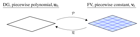
Figure 2: Mapping of the numerical solution between the piecewise polynomials $\bm{u}_{h}$ of the DG scheme and the piecewise constant data $\bm{v}_{h}$ of the finite-volume scheme.

VI Numerical tests

Numerical test cases will be added in the next version of the manuscript.

VII Conclusion and perspectives

We have presented a new causal general relativistic continuum model for dissipative flows which may include flows of viscous fluids as well as elastic and inelastic deformations of solids. The governing PDEs belongs to the class of so-called Symmetric Hyperbolic Thermodynamically Compatible (SHTC) equations and consist of two parts. The non-dissipative part of the PDEs, or the Hamiltonian part, is represented by the hyperbolic time evolution which is derived from the Hamilton principle. The second part, the dissipative one, is represented by algebraic source terms (low order terms) of relaxation type. The resulting system is consistent with the first and second laws of thermodynamics. Thanks to the Hamiltonian nature of the governing equations, the theory is compatible with the Hamiltonian structure of the canonical energy-momentum tensor that appears as the source term in the Einstein field equations.

The main field of the theory is the geometric object, four-distortion field, which is an anholonomic basis tetrad field in differential geometry language. It provides the geometric settings for unified description of flows of fluids and deformation of solids.

Via formal asymptomatic analysis, we demonstrated that the relativistic Navier-Stokes stress tensor is recovered in the leading terms. We also compared our model with the state of the art dissipative relativistic model, the Müller-Israel-Stewart theory, where essential differences were observed in the definition of the stress rate.

The model was discretized using an advanced family of high-order ADER Discontinuous Galerkin (ADER-DG) and ADER Finite Volume (ADER-FO) methods. An extensive range of numerical examples was presented demonstrating the applicability of our theory to relativistic flows of viscous fluids and deformation of solids in Minkowski and curved spacetimes.

Because the SHTC formulation for other transfer process such as mass, heat and electric charge transfer, also admits the Hamiltonian formulation Dumbser et al. (2017); Peshkov et al. (2018), the extension of our Newtonian works is rather a straightforward task, and will be the subject of a near future research. The ultimate goal is to couple this SHTC multi-physic formulation of continuum physics with the recently proposed strongly hyperbolic first-order formulation of the Einstein field equations based on the Conformal and Covariant Z4 system (CCZ4) with constraint-violation damping, which is refereed to as FO-CCZ4 Dumbser et al. (2018), and is implemented in the same ADER-DG framework as the presented model.

Acknowledgment

The research contained in this paper has been financed by the European Research Council (ERC) under the European Union’s Seventh Framework Programme (FP7/2007-2013) with the research project STiMulUs, ERC Grant agreement no. 278267. M.D. and F.F. have further received funding from the European Union’s Horizon 2020 Research and Innovation Programme under the project ExaHyPE, grant agreement number 671698 (call FETHPC-1-2014). E.R. acknowledges a partial support by the Program N15 of the Presidium of RAS, project 121 and the Russian foundation for Basic Research (grant number 16-29-15131). I.P. gratefully acknowledges the support of Agence Nationale de la Recherche (FR) (grant ANR-11-LABX-0040-CIMI) under program ANR-11-IDEX-0002-02. The authors are grateful to the Leibniz Rechenzentrum (LRZ) for awarding access to the SuperMUC supercomputer based in Munich, Germany; they also acknowledge the support of the HLRS computing center for providing access to the Hazel Hen supercomputer based in Stuttgart, Germany. M.D. has received further funding from the Italian Ministry of Education, University and Research (MIUR) in the frame of the Departments of Excellence Initiative 2018–2022 attributed to DICAM of the University of Trento and has been supported by the University of Trento in the frame of the Strategic Initiative Modeling and Simulation.

Appendix A Gravity effect in the Lagrangian description

In this appendix, we explain how the gravity is taken into account in the Lagrangian field equations (36). Because the material coordinates $\xi^{a}$ and metric ${\kappa_{ab}}$ can be assigned in a completely independent manner from their Eulerian counterparts $x^{\mu}$ and $g_{\mu\nu}$, the gravity cannot be associated with the curvature of the Lagrangian manifold $\mathcal{M}^{4}$. In particular, the material metric ${\kappa_{ab}}$ can be taken flat even though the spacetime has a non-vanishing curvature. So, how the gravity effect is accounted for in the Lagrangian description? In fact, the gravity field $g_{\mu\nu}$ is taken into account in the Lagrangian field equations in the fluxes $\Lambda_{x^{\mu}_{\ a}\,}$. Indeed, it is necessary to understand that since our theory is essentially a deformation theory, a single-frame, say pure Lagrangian, description of the matter motion is impossible because two frames are necessary in order to make comparisons of the lengths. Thus, the Lagrangian observer needs to receive some information from a non-comoving observer. The proper Lagrangian strain tensor therefore is (cf. (31))

$$h_{ab}=h_{\mu\nu}x^{\mu}_{\ a}\,x^{\nu}_{\ b}\,$$ (211)

which is the Eulerian projector $h_{\mu\nu}=g_{\mu\nu}+u_{\mu}u_{\nu}$ as seen by the Lagrangian observer. It is then implied that $\Lambda(x^{\mu}_{\ a}\,)=\Lambda(h_{ab})$ (more precisely, it is a function of the invariants of $h_{ab}$) Therefore, the gravity field $g_{\mu\nu}$ emerges in the Lagrangian description not by means of the covariant differentiation but it emerges in the fluxes $\Lambda_{x^{\mu}_{\ a}\,}$ every time when one computes the derivatives

$$\Lambda_{x^{\mu}_{\ a}\,}=\frac{\partial\Lambda}{\partial h_{bc}}\frac{\partial h_{bc}}{\partial x^{\mu}_{\ a}\,}.$$ (212)

Appendix B Orthogonality condition as the consequences of the PDE for $A^{{M}}_{\ \,\mu}$

In this appendix we prove that the orthogonality condition (83b) follows from the way how we define the dissipative source terms in the evolution equation for the distortion field (91b). More precisely, we demonstrate that the relaxation of the time components $A^{{M}}_{\ \,0}$ is rather artificial and is completely defined by the relaxation of the pure matter components $A^{{M}}_{\ \,i}$, $i=1,2,3$. We denote the entire source term (the right hand-side) in (91b) as $S^{{M}}_{\ \,\mu}$ and prove that the distortion field defined as the solution to (91b) fulfills the orthogonality condition (83b) if and only if the source term $S^{{M}}_{\ \mu}$ also satisfies the orthogonality condition

$$S^{{M}}_{\ \mu}u^{\mu}=0,\quad\text{or}\quad S^{{M}}_{\ \,0}=-S^{{M}}_{\ j}\hat{v}^{j},$$ (213)

where $\hat{v}^{j}$ is the pseudo-Newtonian velocity, i.e. $(u^{0},u^{i})=\gamma(1,\hat{v}^{i}):=\gamma(1,\alpha v^{i}-\beta^{i})$, $\gamma=\alpha^{-1}W$, and $v^{i}$ is the Newtonian velocity, $\beta^{i}$ is the shift vector, while $\alpha$ and $W$ are the laps and the Lorentz factor. We note that in the SHTC theory, $S^{{M}}_{\ \mu}\sim\kappa^{{M}{N}}g_{\mu\nu}\mathcal{E}_{A^{{N}}_{\ \,\ \nu}}$ and therefore $S^{{M}}_{\ \mu}$ is indeed orthogonal to $u^{\mu}$ because $\mathcal{E}_{A^{{M}}_{\ \,\mu}}u_{\mu}=0$, see (102).

In the 3+1 notations, orthogonality condition (83b) reads as

$$A^{{M}}_{\ \,0}=-A^{{M}}_{\ \,j}\hat{v}^{j}.$$ (214)

We first prove that if (214) holds then (213) holds as well. Equations (91b) for $\mu=0$ and $\mu=k$ read as

$$\partial_{t}A^{{M}}_{\ \,0}+\hat{v}^{j}\partial_{j}A^{{M}}_{\ \,0}+A^{{M}}_{\ \,j}\partial_{t}\hat{v}^{j}=\gamma^{-1}S^{{M}}_{\ \,0},$$ (215a)

$$\partial_{t}A^{{M}}_{\ \,k}+\hat{v}^{j}\partial_{j}A^{{M}}_{\ \,k}+A^{{M}}_{\ \,j}\partial_{k}\hat{v}^{j}=\gamma^{-1}S^{{M}}_{\ k}.$$ (215b)

After substituting $A^{{M}}_{\ \,0}$ in (215a) by its expression (214), we arrive at

$$-\partial_{t}(A^{{M}}_{\ \,k}\hat{v}^{k})-\hat{v}^{j}\partial_{j}(A^{{M}}_{\ \,k}\hat{v}^{k})+A^{{M}}_{\ \,j}\partial_{t}\hat{v}^{j}=\gamma^{-1}S_{\ \,0}^{M}.$$ (216)

After some term rearrangements, we have

$$-\hat{v}^{k}(\partial_{t}A^{{M}}_{\ \,k}+\hat{v}^{j}\partial_{j}A^{{M}}_{\ \,k})-A^{{M}}_{\ \,k}\hat{v}^{j}\partial_{j}\hat{v}^{k}=\gamma^{-1}S_{\ \,0}^{M}.$$ (217)

Now, substituting the terms in the brackets by (215b), we obtain $S^{{M}}_{\ \,0}=-S^{{M}}_{\ k}\hat{v}^{k}$, i.e. (213) is fulfilled.

We now prove that if (213) holds then (214) is fulfilled. Indeed, assuming (214) is true, equation (215a) can be rewritten as

$$\partial_{t}A^{{M}}_{\ \,0}+\hat{v}^{j}\partial_{j}A^{{M}}_{\ \,0}+A^{{M}}_{\ \,j}\partial_{t}\hat{v}^{j}=-(\partial_{t}A^{{M}}_{\ \,k}+\hat{v}^{j}\partial_{j}A^{{M}}_{\ \,k}+A^{{M}}_{\ \,j}\partial_{k}\hat{v}^{j})\hat{v}^{k}.$$ (218)

After arranging the terms in a proper way, we arrive at

$$\partial_{t}(A^{{M}}_{\ \,0}+A^{{M}}_{\ \,k}\hat{v}^{k})+\hat{v}^{k}\partial_{j}(A^{{M}}_{\ \,0}+A^{{M}}_{\ \,k}\hat{v}^{k})=0,$$ (219)

which means that if (214) holds at the initial moment of time then it holds so at the all later times.

Appendix C Foliation of spacetime $\mathcal{V}^{4}$ and coordinate system

In this section we briefly summarize what means choosing a so called $3+1$ foliation of the spacetime, and choosing a coordinate system on it. Everything in this section is referred mainly to the books by Rezzolla & Zanotti Rezzolla and Zanotti (2013) and Gourgoulhon Gourgoulhon (2012).

C.1 3+1 foliation of $\mathcal{V}^{4}$

First, the 4D space-time is foliated or sliced into a one-parameter family of (non-intersecting) space-like hypersurfaces $\Sigma$ for which a natural parameter is represented by any ’regular’ scalar field $t:\mathcal{V}^{4}\longrightarrow{\rm I\!R}$. The scalar field is enrolled as the time-coordinate since its isosurfaces $\Sigma_{t}$ represent the set of the local events that are simultaneous with the local Eulerian observers.

Given two adjacent leaves $\Sigma_{t}$ and $\Sigma_{t+\delta t}$, there are infinite ways for dragging $\Sigma_{t}$ to $\Sigma_{t+\delta t}$. One way is to select a 4-vector field $n_{\mu}=n_{\mu}(p)$ normal to the hypersurface $\Sigma_{t}$, which is parallel to the gradient of the time-coordinate $\nabla t$, at every event $p\in\Sigma_{t}$. Due to the regularity of the foliation, the time-like vector field $n_{\mu}$ changes smoothly in $t$ and it can be regarded as the tangent vector with respect to a trajectory $\psi\in\mathcal{V}^{4}$. In order to let the trajectory $\psi$ to be compatible with the worldline of a local Eulerian observer, then one choose $n_{\mu}=n_{\mu}(p)$ to be unitary in the sense $n_{\mu}n^{\mu}=-1$. Notice that, this choice allows to interpret $n_{\mu}$ as the 4-velocity of the local Eulerian observer. $n_{\mu}$ is the main building block for the $3+1$ formalism.

C.1.1 Lapse, shift and coordinate system

Then, one defines the normalized 4-vector field at every point $p\in\mathcal{V}^{4}$ as

$$n_{\mu}=-\alpha\nabla_{\mu}t=(-\alpha,0_{i});\quad n^{\mu}n_{\mu}=-1$$ (220)

$$n^{\mu}=\frac{1}{\alpha}(1,-\beta^{i})$$ (221)

where the last identity for the contravariant $n^{\mu}$ is a result of the next definitions. Here we have introduced the so called lapse scalar function $\alpha=\alpha(p)$ and shift spatial-vector $\beta^{\mu}=\beta^{\mu}(p)$. In particular, the lapse function is defined as the inverse of the norm of $\nabla t$, i.e.

$$\alpha:=\left\|\nabla t\right\|^{-1}.$$ (222)

The lapse represents the first arbitrariness of the chosen coordinate system. Then we can define a 4-vector $m_{\mu}:=\alpha n_{\mu}$ that is a non-unitary vector $\left\|m\right\|=-\alpha^{2}$, normal to the hypersurface $\Sigma_{t}$; in particular, vector $\delta t\,m_{\mu}$ drags every event $p\in\Sigma_{t}$ to a corresponding event $p^{\prime}\in\Sigma_{t+\delta t}$; the 4-distance is exactly the proper time

$$\delta\tau_{\mathscr{E}}=\alpha\delta t,$$ (223)

the time measured by the local Eulerian observer; After assigning a purely-spatial coordinate system $\{x^{i}\}$ on each slice $\Sigma_{t}$ that varies ’smoothly’ between any neighbor slices $\Sigma_{t\pm\delta t}$, then the coordinate system $\{t,x^{i}\}$ can be regarded as a well-behaved coordinate system for $\mathcal{V}^{4}$. In this work, the system of coordinates $\{t,x^{i}\}$ is named as ’Eulerian’ system of coordinates. In particular, there exists a natural basis $\{\bm{\partial}_{\mu}\}$ for the tangent space $\mathcal{T}_{p}$ at every event $p\in\mathcal{V}^{4}$, that is associated to the chosen coordinates $\{x_{\mu}\}$. In this notation, the so-called time-vector is defined as $\bm{t}:=\bm{\partial}_{t}$, or $t_{\mu}$ in terms of its coordinates, and it is tangent to the lines of constant spatial coordinates. Similarly to $m_{\mu}$, also $t_{\mu}$ drags the slice $\Sigma_{t}$ to the neighbor one $\Sigma_{t+\delta t}$. It is important to notice that $t_{\mu}$ is not necessarily a timelike vector, and this is the second arbitrariness of the chosen coordinate system. Then, it becomes useful to define the so called shift vector as

$$\beta_{\mu}:=t_{\mu}-m_{\mu}.$$ (224)

By construction, it is spacelike and it lies on the hypersurface $\Sigma_{t}$.

Notice that, any choice of (i) the Eulerian-velocity field $n_{\mu}$, (ii) lapse $\alpha$ and (iii) shift vector $\beta^{i}$ univocally defines the coordinate system $\{t,x^{i}\}$, or atlas, on $\mathcal{V}^{4}$. Vice versa, the specification of a proper atlas on $\mathcal{V}^{4}$ univocally defines the 4-velocities of the Eulerian observers $n_{\mu}$, that are associated to the $t$ isosurfaces, but also the lapse $\alpha$ and shift vector $\beta^{i}$.

The so called Lagrangian coordinate system is obtained after choosing a foliation so that coordinate-lines and the worldlines of the fluid particles and local observers coincide, i.e.

$$\bm{t}(p)\equiv\bm{n}(p)\equiv\bm{u}(p)$$ (225)

for every point in the continuum media $p\in\mathcal{V}^{4}$. In this frame, the time of the coordinates, the proper time as measured by the local observer and the proper time observed by the local fluid particle actually coincide, i.e.

$$t\equiv\tau_{\mathscr{E}}\equiv\tau_{\mathscr{L}}.$$ (226)

C.1.2 Temporal and spatial projectors

The time projection operator and the corresponding (complementary) spatial projection operator are defined as

$$N^{\mu}_{\nu}:=-n^{\mu}n_{\nu},$$ (227)

$$\gamma^{\mu}_{\nu}:=\delta^{\mu}_{\nu}-N^{\mu}_{\nu}=\delta^{\mu}_{\nu}+n^{\mu}n_{\nu}.$$ (228)

These operators allows to split any vector or tensor in its corresponding spatial and time components,

$$U^{\mu}=\gamma^{\mu}_{\nu}U^{\nu}+N^{\mu}_{\nu}U^{\nu}$$ (229)

where the purely spatial vector $V^{\mu}=\gamma^{\mu}_{\nu}U^{\nu}$ is a four-vector with vanishing contravariant time component $V^{0}=0$. Moreover, one can introduce the so called spatial metric $\gamma$

$$\gamma_{\mu\nu}=g_{\mu\nu}-N_{\mu\nu},\quad\gamma^{\mu\nu}=g^{\mu\nu}-N^{\mu\nu}.$$ (230)

allowing to evaluate distances and norms on $\Sigma$, being a purely spatial tensor, i.e. $\gamma^{0\mu}=0$ and $\gamma_{ij}=g_{ij}$ ($\gamma^{ij}\neq g^{ij}$). The explicit form of the covariant and contravariant components of the metric tensor

$$g_{\mu\nu}=\left(\begin{array}[]{cc}-\alpha^{2}+\beta_{i}\beta^{i}&\beta_{i}\\ \beta_{i}&\gamma_{ij}\end{array}\right);g^{\mu\nu}=\left(\begin{array}[]{cc}-1/\alpha^{2}&\beta^{i}/\alpha^{2}\\ \beta^{i}/\alpha^{2}&\gamma^{ij}-\beta^{i}\beta^{j}/\alpha^{2}\end{array}\right).$$ (235)

$$\gamma_{\mu\nu}=\left(\begin{array}[]{cc}\beta_{i}\beta^{i}&\beta_{i}\\ \beta_{i}&\gamma_{ij}\end{array}\right); \gamma^{\mu\nu}=\left(\begin{array}[]{cc}0&0^{i}\\ 0^{i}&\gamma^{ij}\end{array}\right).$$ (240)

One can show further that

$$(-g)^{\frac{1}{2}}=\alpha\gamma^{\frac{1}{2}}.$$ (241)

C.1.3 4-velocity $u_{\mu}$, spatial-velocity $v_{\mu}$ and fluid coordinate velocity $\hat{v}_{\mu}$

There are three different velocities that became useful in simplifying the equations in the text. These velocities are (i) the four-velocity $u_{\mu}$ of a fluid particle, (ii) the spatial four velocity $\mathrm{v}$ and (iii) the fluid coordinate velocity (or transport velocity), defined as

$$(i)\;\;\bm{u}:=\frac{d\bm{p}}{d\tau_{\mathscr{L}}} (ii)\;\;\bm{v}:=\frac{d\bm{\ell}}{d\tau_{\mathscr{E}}} (iii)\;\;\hat{\bm{v}}:=\frac{d\bm{x}}{dt}$$ (242)

Then, the spatial four-velocity $\bm{v}$ as measured by the Eulerian observer of a material particle flowing with four-velocity $\bm{u}$ is

$$v^{\mu}=\frac{\gamma^{\mu}_{\nu}u^{\nu}}{-n_{\alpha}u^{\alpha}}=\frac{\text{proj. of {u} along $\Sigma$}}{\text{Lorentz factor of {u} as measured by {n}}}$$ (243)

$$n_{\alpha}u^{\alpha}=-\alpha u^{0}$$ (244)

and then

$$v^{0} =0,\qquad v^{i}=\frac{\gamma^{i}_{\nu}u^{\nu}}{\alpha u^{0}}=\frac{u^{i}-n^{i}n_{\nu}u^{\nu}}{\alpha u^{0}}=\frac{u^{i}+\alpha n^{i}u^{0}}{\alpha u^{0}}=\frac{u^{i}+\beta^{i}u^{0}}{\alpha u^{0}}=\frac{1}{\alpha}\left(\frac{u^{i}}{u^{0}}+\beta^{i}\right)$$ (245)

$$v_{0} =g_{0\nu}v^{\nu}=\beta_{i}v^{i},\qquad v_{i}=g_{i\nu}v^{\nu}=\beta_{i}v^{0}+\gamma_{ij}v^{j}=\gamma_{ij}v^{j}$$ (246)

Then, from the normalization condition and the definition of Lorentz factor $W$

$$u_{\mu}u^{\mu}=-1,\quad W=-n_{\mu}u^{\mu}=\alpha u^{t}=1/(1-v^{2})$$ (247)

$$u^{t}=\frac{W}{\alpha},\quad u_{t}=W(-\alpha+\beta_{i}v^{i})$$ (248)

one has

$$u^{i}=\frac{W}{\alpha}\left(\alpha v^{i}-\beta^{i}\right)=:\frac{W}{\alpha}\hat{v}^{i}\quad u_{i}=Wv_{i}$$ (249)

$$v^{i}=\frac{u^{i}}{W}+\frac{\beta^{i}}{\alpha},\quad v_{i}=\frac{u_{i}}{W}.$$ (250)

where $\hat{v}$ is named as the fluid coordinate velocity (or transport velocity). Notice moreover

$$u^{\mu}=(\gamma^{\mu}_{\nu}+N^{\mu}_{\nu})u^{\mu}=Wv^{\mu}-(n_{\nu}u^{\nu})n^{\mu}=W(n^{\mu}+v^{\mu})$$ (251)

Appendix D Conservative to primitive transformation

Inspired by the third option of Del Zanna et al. (2007) (simplified since here magnetic fields are absent, actually) we build our strategy for deriving the primitive variables from the conservative set

$$[D,S_{i},U]\longrightarrow[\rho,v_{i},p]$$ (252)

$$D =\rho W,$$ (253)

$$S_{i} =\rho hW^{2}v_{i}+\alpha\Sigma^{0}_{\hphantom{\mu}i}=\rho hW^{2}v_{i}+\sigma_{i},$$ (254)

$$U =\rho hW^{2}-p+\alpha^{2}\Sigma^{00}=\rho hW^{2}-p+\sigma$$ (255)

Then we guess the initial value of

$$\sigma_{i}=v^{j}\Sigma_{ij},\quad\text{and}\quad\sigma=v^{i}v^{j}\Sigma_{ij}$$ (256)

and look for the roots of two auxiliary functions

$$x:=v^{2}, F_{1}(x,y) :=y^{2}\,x-\tilde{S}^{2},$$ (257)

$$y:=\rho hW^{2}, F_{2}(x,y) :=y-p-\tilde{U},$$ (258)

after defining the four vector and the scalar

$$\tilde{S}_{\mu}:=S_{\mu}-\sigma_{\mu},\quad\tilde{U}:=U-\sigma$$ (259)

Notice that guess of the couple $(\sigma_{i},\sigma)$ can be substituted by an initial guess $(\rho,v)$ or $(\rho,\hat{v})$, that are used for evaluating a corresponding initial state of $(\sigma_{i},\sigma)$. Introducing the definition of enthalpy

$$h=1+e_{0}+e_{1}+\frac{p}{\rho}$$ (260)

where, after assuming

$$p(\rho,e_{0})=(\gamma-1)\rho e_{0}\quad\Rightarrow\quad h=1+e_{1}+\frac{\gamma}{\gamma-1}\frac{p}{\rho}$$ (261)

and, since $\rho h=y/W^{2}=y(1-x)$, then

$$p=\frac{\gamma-1}{\gamma}\left[\rho h-\rho(1+e_{1})\right]=\frac{\gamma-1}{\gamma}\left[y(1-x)-D(1+e_{1})(1-x)^{\frac{1}{2}}\right].$$ (262)

Using 258, we have the roots

$$y =p+\tilde{U}=\frac{\gamma-1}{\gamma}y(1-x)-\frac{\gamma-1}{\gamma}D(1+e_{1})(1-x)^{\frac{1}{2}}+\tilde{U}$$ (263)

$$=-\left[1-\frac{\gamma-1}{\gamma}(1-x)\right]^{-1}\left[\frac{\gamma-1}{\gamma}D(1+e_{1})(1-x)^{\frac{1}{2}}-\tilde{U}\right],$$ (264)

$$x =\tilde{S}^{2}/y^{2}$$ (265)

In practice, if we use $D(1+e_{1})$ instead of $D$ we may recycle the same subroutine of GRMHD.
An alternative could be the following: re-define the four vector and the scalar

$$\tilde{S}_{\mu} :=S_{\mu}-\sigma_{\mu}-\rho e_{1}W^{2}v_{i},$$ (266)

$$\tilde{U} :=U-\sigma-\rho e_{1}W^{2}$$ (267)

$$x :=v^{2},$$ (268)

$$y :=\rho(h-e_{1})W^{2}$$ (269)

and one obtains

$$y =-\left[1-\frac{\gamma-1}{\gamma}(1-x)\right]^{-1}\left[\frac{\gamma-1}{\gamma}D(1-x)^{\frac{1}{2}}-\tilde{U}\right],$$ (270)

$$x =\tilde{S}^{2}/y^{2}$$ (271)

References

- Rezzolla and Zanotti (2013) L. Rezzolla and O. Zanotti, Relativistic hydrodynamics (Oxford University Press, Oxford, 2013).
- Carter and Quintana (1972) B. Carter and H. Quintana, Proceedings of the Royal Society A: Mathematical, Physical and Engineering Sciences 331, 57 (1972).
- Kijowski and Magli (1992) J. Kijowski and G. Magli, Journal of Geometry and Physics 9, 207 (1992).
- Karlovini and Samuelsson (2003) M. Karlovini and L. Samuelsson, Classical and Quantum Gravity (2003), 10.1088/0264-9381/22/4/C02, arXiv:0211026 [gr-qc] .
- Wernig-Pichler (2006) M. Wernig-Pichler, Thesis, Ph.D. thesis, Institut für theoretische Physik der Universität Wien (2006), arXiv:0605025 [gr-qc] .
- Broda (2008) S. Broda, Comparison of two different formalisms for relativistic elasticity theory, Ph.D. thesis, University of Vienna (2008).
- Gundlach et al. (2012) C. Gundlach, I. Hawke, and S. J. Erickson, Classical and Quantum Gravity 29, 015005 (2012), arXiv:1107.2551 .
- de Groot and Mazur (1984) S. R. de Groot and P. Mazur, Non-equilibrium Thermodynamics, Dover Books on Physics (Dover Publications, 1984).
- Lebon et al. (2008) G. Lebon, D. Jou, and J. Casas-Vázquez, Understanding Non-equilibrium Thermodynamics (Springer Berlin Heidelberg, Berlin, Heidelberg, 2008).
- Hiscock and Lindblom (1988) W. A. Hiscock and L. Lindblom, Physics Letters A 131, 509 (1988).
- Romatschke (2010) P. Romatschke, International Journal of Modern Physics E 19(1), 1 (2010).
- Schaeffer (1987) D. G. Schaeffer, Journal of Differential Equations 66, 19 (1987).
- Barker et al. (2015) T. Barker, D. G. Schaeffer, P. Bohorquez, and J. M. N. T. Gray, J. Fluid Mech 779, 794 (2015).
- Eckart (1940) C. Eckart, Physical Review 58, 919 (1940), arXiv:arXiv:1011.1669v3 .
- Landau and Lifshitz (1966) L. D. Landau and E. M. Lifshitz, Fluid Mechanics, Course of Theoretical Physics, Volume 6 (Pergamon Press, 1966).
- Van and Biro (2012) P. Van and T. S. Biro, Physics Letters, Section B: Nuclear, Elementary Particle and High-Energy Physics 709, 106 (2012), arXiv:1109.0985 .
- Freistühler and Temple (2017) H. Freistühler and B. Temple, Proceedings of the Royal Society A 473 (2017).
- Hughes et al. (1977) T. J. R. Hughes, T. Kato, and J. E. Marsden, Archive for Rational Mechanics and Analysis 63, 273 (1977).
- Maxwell (1867) J. C. Maxwell, Philosophical Transactions of the Royal Society of London , 49 (1867).
- Cattaneo (1948) C. Cattaneo, Atti sem. Mat. Fis. Univ. Modena 3 (1948).
- Mueller (1966) I. Mueller, Zur Ausbreitungsgeschwindigkeit von Störungen in kontinuierlichen Medien, Ph.D. thesis, RWTH Aachen University, Aachen (1966).
- Muller (1967) I. Muller, Z. Phys. 198, 329 (1967).
- Israel (1976) W. Israel, Annals of Physics 100, 310 (1976).
- Stewart (1977) J. M. Stewart, Proceedings of the Royal Society A: Mathematical, Physical and Engineering Sciences 357, 59 (1977).
- Grad (1949) H. Grad, Communications on Pure and Applied Mathematics 2, 331 (1949).
- Torrilhon (2016) M. Torrilhon, Annual Review of Fluid Mechanics 48, 429 (2016).
- Liu et al. (1986) I.-S. Liu, I. Müller, and T. Ruggeri, Annals of Physics 169, 191 (1986).
- Muller and Ruggeri (1998) I. Muller and T. Ruggeri, Rational Extended Thermodynamics, Vol. 16 (Springer, 1998).
- Ruggeri and Sugiyama (2015) T. Ruggeri and M. Sugiyama, Rational Extended Thermodynamics beyond the Monatomic Gas (Springer, 2015) pp. 1–376.
- Geroch and Lindblom (1990) R. Geroch and L. Lindblom, “Dissipative relativistic fluid theories of divergence type,” (1990).
- Lehner et al. (2017) L. Lehner, O. A. Reula, and M. E. Rubio, Physical Review D 97, 24013 (2017), arXiv:1710.08033 .
- Jou et al. (2010) D. Jou, J. Casas-Vázquez, and G. Lebon, Extended irreversible thermodynamics (Springer Berlin Heidelberg, Dordrecht, 2010).
- Andersson and Comer (2007) N. Andersson and G. L. Comer, Living Reviews in Relativity 10 (2007), 10.12942/lrr-2007-1, arXiv:0605010 [gr-qc] .
- Bouras et al. (2009) I. Bouras, E. Molnár, H. Niemi, Z. Xu, A. El, O. Fochler, C. Greiner, and D. H. Rischke, Physical Review Letters 103, 741 (2009), arXiv:arXiv:0907.4519v2 .
- Bouras et al. (2010) I. Bouras, E. Molnár, H. Niemi, Z. Xu, A. El, O. Fochler, C. Greiner, and D. H. Rischke, Physical Review C - Nuclear Physics 82, 1 (2010), arXiv:1006.0387 .
- Takamoto and ichiro Inutsuka (2011) M. Takamoto and S. ichiro Inutsuka, Journal of Computational Physics 230, 7002 (2011), arXiv:1106.1732 .
- Akamatsu et al. (2014) Y. Akamatsu, S.-i. Inutsuka, C. Nonaka, and M. Takamoto, Journal of Computational Physics 256, 34 (2014).
- Del Zanna et al. (2013) L. Del Zanna, V. Chandra, G. Inghirami, V. Rolando, A. Beraudo, A. De Pace, G. Pagliara, A. Drago, and F. Becattini, The European Physical Journal C 73, 2524 (2013).
- Karpenko et al. (2014) I. Karpenko, P. Huovinen, and M. Bleicher, Computer Physics Communications 185, 3016 (2014), arXiv:arXiv:1312.4160v1 .
- Shen et al. (2016) C. Shen, Z. Qiu, H. Song, J. Bernhard, S. Bass, and U. Heinz, Computer Physics Communications 199, 61 (2016).
- Chamel and Haensel (2008) N. Chamel and P. Haensel, Living Reviews in Relativity 11, 10 (2008).
- Schaerer and Torrilhon (2017) R. P. Schaerer and M. Torrilhon, European Journal of Mechanics - B/Fluids 64, 30 (2017).
- Denicol et al. (2012a) G. S. Denicol, E. Molnár, H. Niemi, and D. H. Rischke, European Physical Journal A 48, 1 (2012a), arXiv:1206.1554 .
- Peshkov and Romenski (2016) I. Peshkov and E. Romenski, Continuum Mechanics and Thermodynamics 28, 85 (2016).
- Dumbser et al. (2016) M. Dumbser, I. Peshkov, E. Romenski, and O. Zanotti, Journal of Computational Physics 314, 824 (2016), arXiv:1511.08995 .
- Dumbser et al. (2017) M. Dumbser, I. Peshkov, E. Romenski, and O. Zanotti, Journal of Computational Physics 348, 298 (2017), arXiv:1612.02093 .
- Peshkov et al. (2017) I. Peshkov, E. Romenski, and M. Dumbser, To appear in Springer Proceedings in Mathematics and Statistics, XVI International Conference on Hyperbolic Problems (2017), arXiv:1705.02151 .
- Peshkov et al. (2019a) I. Peshkov, E. Romenski, and M. Dumbser, Continuum Mechanics and Thermodynamics (2019a), 10.1007/s00161-019-00770-6, arXiv:1810.03761 .
- Godunov and Romenskii (1974) S. K. Godunov and E. I. Romenskii, Journal of Applied Mechanics and Technical Physics 13, 868 (1974).
- Godunov (1978) S. K. Godunov, Elements of mechanics of continuous media, 1st ed. (Nauka, 1978).
- Romenskii (1979) E. I. Romenskii, Journal of Applied Mechanics and Technical Physics 20, 229 (1979).
- Godunov and Romensky (1995) S. Godunov and E. Romensky, in Computational Fluid Dynamics Review 1995, Vol. 95 (John Wiley, NY, 1995) pp. 19–31.
- Godunov and Romensky (1996) S. K. Godunov and E. I. Romensky, in ECCOMAS Conference on numerical methods in engineering (1996) pp. 54–57.
- Godunov and Romenskii (2003) S. K. Godunov and E. I. Romenskii, Elements of continuum mechanics and conservation laws (Kluwer Academic/Plenum Publishers, 2003).
- Besseling (1968) J. F. Besseling, in Irreversible Aspects of Continuum Mechanics and Transfer of Physical Characteristics in Moving Fluids, IUTAM Symposia, edited by H. Parkus and L. I. Sedov (Springer Vienna, 1968) pp. 16–53.
- Besseling and Van Der Giessen (1994) J. F. Besseling and E. Van Der Giessen, Mathematical Modelling of Inelastic Deformation (Springer US, Boston, MA, 1994).
- Rubin (1987) M. Rubin, International Journal of Engineering Science 25, 1175 (1987).
- Rubin (2019) M. B. Rubin, Philosophical Transactions of the Royal Society A: Mathematical, Physical and Engineering Sciences 377, 20180071 (2019).
- Frenkel (1955) J. Frenkel, Kinetic theory of liquids (Dover, 1955).
- Brazhkin et al. (2012) V. V. Brazhkin, Y. D. Fomin, A. G. Lyapin, V. N. Ryzhov, and K. Trachenko, Physical Review E 85, 31203 (2012).
- Bolmatov et al. (2013) D. Bolmatov, V. V. Brazhkin, and K. Trachenko, Nature communications 4, 1 (2013).
- Bolmatov et al. (2015a) D. Bolmatov, M. Zhernenkov, D. Zav’yalov, S. Stoupin, Y. Q. Cai, and A. Cunsolo, The journal of physical chemistry letters 6, 3048 (2015a).
- Bolmatov et al. (2015b) D. Bolmatov, D. Zav’yalov, M. Zhernenkov, E. T. Musaev, and Y. Q. Cai, Annals of Physics 363, 221 (2015b), arXiv:arXiv:1512.07191v1 .
- Bolmatov et al. (2016) D. Bolmatov, M. Zhernenkov, D. Zav’yalov, S. Stoupin, A. Cunsolo, and Y. Q. Cai, Scientific Reports 6, 19469 (2016), arXiv:arXiv:1601.03568v1 .
- Peshkov et al. (2019b) I. Peshkov, W. Boscheri, R. Loubère, E. Romenski, and M. Dumbser, Journal of Computational Physics 387, 481 (2019b), arXiv:1806.00706 .
- Peshkov et al. (2018) I. Peshkov, M. Pavelka, E. Romenski, and M. Grmela, Continuum Mechanics and Thermodynamics (2018), 10.1007/s00161-018-0621-2, arXiv:1710.00058 .
- Godunov (1961) S. K. Godunov, Dokl. Akad. Nauk SSSR 139(3), 521 (1961).
- Godunov (1972) S. K. Godunov, Numerical Methods for Mechanics of Continuum Medium 3, 26 (1972).
- Godunov et al. (1996) S. Godunov, T. Yu Mikhailova, and E. Romenskii, Siberian Mathematical Journal 37, 790 (1996).
- Romensky (1998) E. I. Romensky, Mathematical and computer modelling 28, 115 (1998).
- Romensky (2001) E. I. Romensky, in Godunov Methods: Theory and Applications, edited by E. Toro (Springer US, New York, 2001) pp. 745–761.
- Carter (1991) B. Carter, Proceedings: Mathematical and Physical Sciences 433, 45 (1991).
- Andersson and Comer (2015) N. Andersson and G. L. Comer, Classical and Quantum Gravity 32, 75008 (2015), arXiv:1306.3345 .
- Grmela and Öttinger (1997) M. Grmela and H. C. Öttinger, Physical Review E 56, 6620 (1997).
- Öttinger and Grmela (1997) H. C. Öttinger and M. Grmela, Physical Review E 56, 6633 (1997).
- Öttinger (1998a) H. C. Öttinger, Physica A: Statistical Mechanics and its Applications 259, 24 (1998a).
- Öttinger (1998b) H. C. Öttinger, Physica A: Statistical Mechanics and its Applications 254, 433 (1998b).
- Öttinger (2005) H. C. Öttinger, Beyond Equilibrium Thermodynamics (John Wiley & Sons, Inc., 2005) p. 656.
- Pavelka et al. (2018) M. Pavelka, V. Klika, and M. Grmela, Multiscale Thermo-Dynamics (De Gruyter, Berlin, Boston, 2018).
- Stricker and Öttinger (2019) L. Stricker and H. C. Öttinger, Physical Review E 99, 013105 (2019), arXiv:1809.04956 .
- Hiscock and Lindblom (1983) W. A. Hiscock and L. Lindblom, Annals of Physics 151, 466 (1983).
- Hiscock and Lindblom (1985) W. A. Hiscock and L. Lindblom, Physical Review D 31, 725 (1985).
- Bobylev (1982) A. Bobylev, Akademiia Nauk SSSR Doklady 262, 71 (1982).
- Struchtrup and Torrilhon (2003) H. Struchtrup and M. Torrilhon, Physics of Fluids 15, 2668 (2003).
- Ruggeri and Strumia (1981) T. Ruggeri and A. Strumia, Ann. Inst. Henri Poincaré 34, 65 (1981).
- Sedov (1971) L. Sedov, A course in continuum mechanics. Volume I. Basic equations and analytical techniques (Wolters-Noordhoff Publishing, Groningen, 1971).
- Maugin (1974) G. A. Maugin, General Relativity and Gravitation 5, 13 (1974).
- Godunov and Romenskii (1972) S. K. Godunov and E. I. Romenskii, Journal of Applied Mechanics and Technical Physics 13(6), 868 (1972).
- Katanaev and Volovich (1992) M. O. Katanaev and I. V. Volovich, Annals of Physics 216, 1 (1992).
- Gavrilyuk (2011) S. Gavrilyuk, in Variational Models and Methods in Solid and Fluid Mechanics. CISM Courses and Lectures, vol 535 (Springer, Vienna, Vienna, 2011) springer ed., pp. 163–210.
- Friedrichs (1958) K. O. Friedrichs, Communications on Pure and Applied Mathematics1 11, 333 (1958).
- Boillat (1974) G. Boillat, C. R. Acad. Sc. Paris, Sér A 278 (1974).
- Godunov and Peshkov (2010) S. Godunov and I. Peshkov, Computational Mathematics and Mathematical Physics 50, 1409 (2010).
- Kijowski et al. (1990) J. Kijowski, A. Smólski, and A. Górnicka, Physical Review D 41 (1990).
- Kijowski and Magli (1998) J. Kijowski and G. Magli, Classical and Quantum Gravity 15, 3891 (1998).
- Maugin (1972) G. A. Maugin, Annales de l’I.H.P. Physique théorique 16, 133 (1972).
- Beig and Schmidt (2003) R. Beig and B. G. Schmidt, Classical and Quantum Gravity 20, 889 (2003), arXiv:0211054 [gr-qc] .
- Kleinert (2008) H. Kleinert, Multivalued Fields (World Scientific, 2008).
- Landau and Lifshitz (2004) L. D. Landau and E. M. Lifshitz, Fluid Mechanics, Course of Theoretical Physics, Volume 6 (Elsevier Butterworth-Heinemann, Oxford, 2004).
- Huovinen and Molnar (2009) P. Huovinen and D. Molnar, PHYSICAL REVIEW C 79 (2009), 10.1103/PhysRevC.79.014906.
- Denicol et al. (2012b) G. S. Denicol, H. Niemi, E. Molnár, and D. H. Rischke, Physical Review D 85, 1 (2012b).
- Pavelka et al. (2016) M. Pavelka, V. Klika, O. Esen, and M. Grmela, Physica D: Nonlinear Phenomena 335, 54 (2016).
- Jackson and Nikiforakis (2019) H. Jackson and N. Nikiforakis, Journal of Computational Physics 387, 410 (2019), arXiv:1811.04766 .
- Dumbser et al. (2014a) M. Dumbser, O. Zanotti, R. Loubère, and S. Diot, Journal of Computational Physics 278, 47 (2014a).
- Zanotti et al. (2015a) O. Zanotti, F. Fambri, M. Dumbser, and A. Hidalgo, Computers and Fluids 118, 204 (2015a).
- Zanotti et al. (2015b) O. Zanotti, F. Fambri, and M. Dumbser, Mon. Not. R. Astron. Soc. 452, 3010 (2015b).
- Fambri et al. (2017) F. Fambri, M. Dumbser, and O. Zanotti, Computer Physics Communications 220, 297 (2017).
- Fambri et al. (2018) F. Fambri, M. Dumbser, S. Köppel, L. Rezzolla, and O. Zanotti, Monthly Notices of the Royal Astronomical Society , sty734 (2018).
- Toro (2009) E. F. Toro, {Riemann} Solvers and Numerical Methods for Fluid Dynamics, 3rd ed. (Springer, 2009).
- Parés (2006) C. Parés, SIAM Journal on Numerical Analysis 44, 300 (2006).
- Castro et al. (2006) M. J. Castro, J. M. Gallardo, and C. Parés, Mathematics of Computation 75, 1103 (2006).
- Castro et al. (2017) M. J. Castro, T. de Luna, and C. Parés, in Handbook of Numerical Methods for Hyperbolic Problems, Handbook of Numerical Analysis, Vol. 18, edited by R. Abgrall and C.-W. Shu (Elsevier, 2017) pp. 131–175.
- Parés (2010) C. Parés, in Numerical Methods for Balance Laws, Quaderni di matematica, edited by G. Puppo and G. Russo (Aracne, 2010) pp. 67–122.
- Parés and Muñoz-Ruiz (2009) C. Parés and M. L. Muñoz-Ruiz, Bol. Soc. Esp. Mat. Apl. 47, 19 (2009).
- Dal Maso et al. (1995) G. Dal Maso, P. LeFloch, and F. Murat, Journal de mathématiques pures et appliquées 74, 483 (1995).
- Dumbser et al. (2009) M. Dumbser, M. Castro, C. Parés, and E. F. Toro, Computers and Fluids 38, 1731 (2009).
- Dumbser and Toro (2011) M. Dumbser and E. F. Toro, Journal of Scientific Computing 48, 70 (2011).
- Rusanov (1961) V. V. Rusanov, J. Comput. Math. Phys. USSR 1, 267 (1961).
- Dumbser and Balsara (2016) M. Dumbser and D. S. Balsara, Journal of Computational Physics 304, 275 (2016).
- Dumbser et al. (2008) M. Dumbser, D. Balsara, E. F. Toro, and C. D. Munz, Journal of Computational Physics 227, 8209 (2008).
- Dumbser et al. (2013) M. Dumbser, O. Zanotti, A. Hidalgo, and D. S. Balsara, Journal of Computational Physics 248, 257 (2013).
- Dumbser et al. (2014b) M. Dumbser, A. Hidalgo, and O. Zanotti, Computer Methods in Applied Mechanics and Engineering 268, 359 (2014b).
- Godunov (1959) S. Godunov, Mat. Sb. 47, 271 (1959).
- Clain et al. (2011) S. Clain, S. Diot, and R. Loubère, Journal of Computational Physics 230, 4028 (2011).
- Diot et al. (2012) S. Diot, S. Clain, and R. Loubère, Computers and Fluids 64, 43 (2012).
- Diot et al. (2013) S. Diot, R. Loubère, and S. Clain, International Journal of Numerical Methods in Fluids 73, 362 (2013).
- Loubère et al. (2014) R. Loubère, M. Dumbser, and S. Diot, Communication in Computational Physics 16, 718 (2014).
- Boscheri and Dumbser (2017) W. Boscheri and M. Dumbser, Journal of Computational Physics 346, 449 (2017).
- Schlichting and Gersten (2005) H. Schlichting and K. Gersten, Grenzschicht-theorie (Springer Verlag, 2005).
- Michel (1972) F. C. Michel, Astrophys. Spa. Sci. 15, 153 (1972).
- Komissarov (2004) S. S. Komissarov, Mon. Not. R. Astron. Soc. 350, 1431 (2004).
- Dumbser et al. (2018) M. Dumbser, F. Guercilena, S. Köppel, L. Rezzolla, and O. Zanotti, Physical Review D 97, 084053 (2018), arXiv:1707.09910 .
- Gourgoulhon (2012) E. Gourgoulhon, Lecture Notes in Physics, Lecture Notes in Physics, Vol. 846 (Berlin Springer Verlag, 2012).
- Del Zanna et al. (2007) L. Del Zanna, O. Zanotti, N. Bucciantini, and P. Londrillo, Astronomy & Astrophysics 473, 11 (2007), arXiv:0704.3206 .