Compositional Generalization for Primitive Substitutions

Abstract

Compositional generalization is a basic mechanism in human language learning, but current neural networks lack such ability. In this paper, we conduct fundamental research for encoding compositionality in neural networks. Conventional methods use a single representation for the input sentence, making it hard to apply prior knowledge of compositionality. In contrast, our approach leverages such knowledge with two representations, one generating attention maps, and the other mapping attended input words to output symbols. We reduce the entropy in each representation to improve generalization. Our experiments demonstrate significant improvements over the conventional methods in five NLP tasks including instruction learning and machine translation. In the SCAN domain, it boosts accuracies from 14.0% to 98.8% in Jump task, and from 92.0% to 99.7% in TurnLeft task. It also beats human performance on a few-shot learning task. We hope the proposed approach can help ease future research towards human-level compositional language learning. Source code is available online.

1 Introduction

Humans learn language in a flexible and efficient way by leveraging systematic compositionality, the algebraic capacity to understand and produce large amount of novel combinations from known components Chomsky (1957); Montague (1970). For example, if a person knows how to “step”, “step twice” and “jump”, then it is natural for the person to know how to “jump twice” (Figure 1). This compositional generalization is critical in human cognition Minsky (1986); Lake et al. (2017), and it helps humans learn language from a limited amount of data, and extend to unseen sentences.

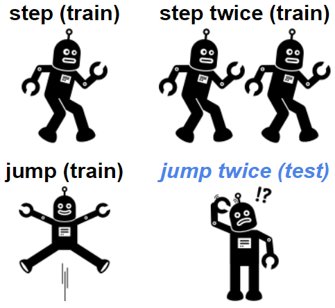
Figure 1: Problem illustration. If a person knows how to “step”, “step twice” and “jump”, then the person should know how to “jump twice”. Although this is straightforward for humans, it remains an open problem to equip machines with such ability.

In recent years, deep neural networks have made many breakthroughs in various problems LeCun et al. (2015); Krizhevsky et al. (2012); Yu and Deng (2012); He et al. (2016); Wu and et al (2016). However, there have been critiques that neural networks do not have compositional generalization ability Fodor and Pylyshyn (1988); Marcus (1998); Fodor and Lepore (2002); Marcus (2003); Calvo and Symons (2014).

jump	JUMP
run after run left	LTURN RUN RUN
look left twice and look opposite right	LTURN LOOK LTURN LOOK RTURN
	RTURN LOOK
jump twice after look	LOOK JUMP JUMP
turn left after jump twice	JUMP JUMP LTURN
jump right twice after jump left twice	LTURN JUMP LTURN JUMP RTURN JUMP
	RTURN JUMP

(a) Jump task. In training, “jump” only appears as a single command. In test, it appears with other words.

turn left	LTURN
run thrice and jump right	RUN RUN RUN RTURN JUMP
look left thrice after run left twice	LTURN RUN LTURN RUN LTURN
	LOOK LTURN LOOK LTURN LOOK
look twice and turn left twice	LOOK LOOK LTURN LTURN
turn left thrice and turn left	LTURN LTURN LTURN LTURN
turn left twice after look opposite right twice	RTURN RTURN LOOK RTURN
	RTURN LOOK LTURN LTURN

(b) TurnLeft task. In training, “turn left” only appears as a single command. In test, it appears with other words.

Table 1: Examples of SCAN input commands (left) and output action sequences (right). Upper section is for training, and lower section is for testing. These tasks are difficult because “jump” (or “turn left”) does not appear with other words in training.

Our observation is that conventional methods use a single representation for the input sentence, which makes it hard to apply prior knowledge of compositionality. In contrast, our approach leverages such knowledge with two representations, one generating attention maps, and the other mapping attended input words to output symbols. We reduce each of their entropies to improve generalization. This mechanism equips the proposed approach with the ability to understand and produce novel combinations of known words and to achieve compositional generalization.

In this paper, we focus on compositinal generalization for primitive substitutions. We use Primitive tasks in the SCAN Lake and Baroni (2018) dataset—a set of command-action pairs—for illustrating how the proposed algorithm works. In a Primitive task, training data include a single primitive command, and other training commands do not contain the primitive. In test data, the primitive appears together with other words. A primitive can be “jump” (Jump, see Table 1(a) for examples) or “turn left” (TurnLeft, see Table 1(b) for examples). These tasks are difficult because “jump” (or “turn left”) does not appear with other words in training. A model without compositionality handling will easily learn a wrong rule such as “any sentence with more than one word should not contain the ‘jump’ action”. This rule fits the training data perfectly, and may reduce training loss quickly, but it does not work for test data. In contrast, our algorithm can process a sentence such as “jump twice after look” correctly by generating a sequence of three attention maps from function representation and then a sequence of actions “LOOK JUMP JUMP” by decoding the primitive representation from the attended command words (see the example in Figure 2).

Besides Primitive tasks, we experiment on more tasks in SCAN and other datasets for instruction learning and machine translation. We also introduce an extension of SCAN dataset, dubbed as SCAN-ADJ, which covers additional compositional challenges. Our experiments demonstrate that the proposed method achieves significant improvements over the conventional methods. In the SCAN domain, it boosts accuracies from 14.0% to 98.8% in Jump task, and from 92.0% to 99.7% in TurnLeft task. It also beats human performance on a few-shot learning task.

2 Approach

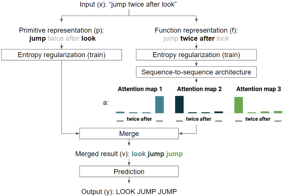
Figure 2: Illustration of network structure and flowchart for the proposed approach. Input is a sequence of words. Output is a sequence of actions. An input sentence is converted to primitive representation (left) and function representation (right). In training, we reduce entropy of two representations. Function representation is used to generate a sequence of attention maps. Each attention map is used to select an embedding from primitive representation to output an action.

In compositional generalization tasks, we consider both input $X$ and output $Y$ have multiple components that are not labeled in data. Suppose input has two components $X_{1}$ and $X_{2}$, and output has two components $Y_{1}$ and $Y_{2}$, then we can define compositional generalization probabilistically as follows. In training,

$$P(X_{1})>0\text{ and }P(X_{2})>0,$$

$$P(X_{1},X_{2})=0,$$

$$P(Y_{1}|X_{1})\text{ and }P(Y_{2}|X_{2})\text{ are high.}$$

In test,

$$P(X_{1},X_{2})>0,$$

$$P(Y_{1},Y_{2}|X_{1},X_{2})\text{ is predicted high.}$$

We expect this is possible when we have prior knowledge that $Y_{1}$ depends only on $X_{1}$ and $Y_{2}$ depends only on $X_{2}$.

$$P(Y_{1}|X_{1},X_{2},Y_{2})=P(Y_{1}|X_{1}),$$

$$P(Y_{2}|X_{1},X_{2},Y_{1})=P(Y_{2}|X_{2}).$$

Therefore, with chain rule,

$$P(Y_{1},Y_{2}|X_{1},X_{2})=P(Y_{1}|X_{1})P(Y_{2}|X_{2}).$$

Since $P(Y_{1}|X_{1})$ and $P(Y_{2}|X_{2})$ are both high in training, if they generalize well, they should also be high in test, so that their product should be high in test. To make $P(Y_{1}|X_{1})$ and $P(Y_{2}|X_{2})$ generalize well at test time, we hope to remove unnecessary information from $X_{1}$ and $X_{2}$. In other words, we want $X_{1}$ ($X_{2}$) to be a minimal sufficient statistic for $Y_{1}$ ($Y_{2}$).

In this task, input $X$ is a word sequence, and output $Y$ is an action sequence. We consider $X$ has two types of information: which actions are present ($X_{1}$), and how the actions should be ordered ($X_{2}$). $Y$ is constructed by the output action types ($Y_{1}$), and output action order ($Y_{2}$). $Y_{1}$ depends only on $X_{1}$, and $Y_{2}$ depends only on $X_{2}$.

Based on these arguments, we design the algorithm with the following objectives:

1. Learn two representations for input.

2. Reduce entropy in each representation.

3. Make output action type depend only on one representation, and output action order depend only on the other.

Figure 2 shows an illustration of flowchart for the algorithm design (see Algorithm 1 for details). We describe it further here.

Algorithm 1 Proposed approach. Decoder in Seq2seq architecture is autoregressive model here.

1:$V$: output vocabulary size

2:        $k_{p},k_{f}$: embedding sizes

3:        $\alpha$: 1 for training, 0 for inference

4:        Seq2seq: seq2seq architecture

5:$x$: sequence of one-hot representations

6:$\hat{y}$: sequence of distributions

7:for $i=1,\dots,n$ do

8:   $p_{i}=\text{Emb}_{p}(x_{i})\in\mathbb{R}^{k_{p}}$

9:   $f_{i}=\text{Emb}_{f}(x_{i})\in\mathbb{R}^{k_{f}}$

10:end for

11:$p^{\prime}=p+\alpha\epsilon_{p}\in\mathbb{R}^{n\times k_{p}},\epsilon_{p}\sim\mathcal{N}(0,I)$

12:$f^{\prime}=f+\alpha\epsilon_{f}\in\mathbb{R}^{n\times k_{f}},\epsilon_{f}\sim\mathcal{N}(0,I)$

13:$\text{decoder}=\text{Seq2seq}(f^{\prime})$

14:for $j=1,\dots,$ max length do

15:   $b_{j}=\text{decoder.next()}\in\mathbb{R}^{n}$

16:   $a_{j}=\text{Softmax}(b_{j})\in\mathbb{R}^{n}$

17:   $v_{j}=a_{j}p^{\prime}\in\mathbb{R}^{k_{p}}$

18:   $l_{j}=f_{\text{predict}}(v_{j})\in\mathbb{R}^{V}$

19:   $\hat{y}_{j}=\text{Softmax}(l_{j})\in(0,1)^{V}$

20:   break if $\operatorname*{\arg\!\max}{\hat{y}_{j}}$ is <EOS>

21:end for

2.1 Input and Output

Input $x$ contains a sequence of $n$ words, where each input word is from an input vocabulary of size $U$. Output $y$ contains a sequence of $m$ action symbols, where each output symbol is from an output vocabulary of size $V$. Both vocabularies contain an end-of-sentence symbol which appears at the end of $x$ and $y$, respectively. The model output $\hat{y}$ is a prediction for $y$. Both input words and output symbols are in one-hot representation, i.e.,

$$\begin{split}&x=[x_{1},\dots,x_{n}]\in\{0,1\}^{U\times n},\\ &y=[y_{1},\dots,y_{m}]\in\{0,1\}^{V\times m}.\end{split}$$

2.2 Primitive Representation and Function Representation

To achieve objective (i), we use two representations for an input sentence. For each word, we use two word embeddings for primitive and functional information.

$$\begin{split}&p_{i}=\text{Emb}_{p}(x_{i})\in\mathbb{R}^{k_{p}},\\ &f_{i}=\text{Emb}_{f}(x_{i})\in\mathbb{R}^{k_{f}}.\end{split}$$

We concatenate $p_{i}$ and $f_{i}$ to form the primitive representation and functional representation for the entire input sequence, i.e.,

$$\begin{split}&p=[p_{1},\dots,p_{n}]\in\mathbb{R}^{k_{p}\times n},\\ &f=[f_{1},\dots,f_{n}]\in\mathbb{R}^{k_{f}\times n}.\end{split}$$

2.3 Entropy Regularization

To achieve objective (ii), we reduce the amount of information, or entropy of the representations. We do this by regularizing the $L_{2}$ norm of the representations, and then adding noise to them. This reduces channel capacities, and thus entropy for the representations.

$$\begin{split}&p^{\prime}=p+\alpha\epsilon_{p}\in\mathbb{R}^{k_{p}\times n},\epsilon_{p}\sim\mathcal{N}(0,I),\\ &f^{\prime}=f+\alpha\epsilon_{f}\in\mathbb{R}^{k_{f}\times n},\epsilon_{f}\sim\mathcal{N}(0,I),\\ &\mathcal{L}_{\text{regularize}}=L_{2}(p)+L_{2}(f).\end{split}$$

Here, $\alpha$ is the weight for noise. Noise is helpful in training, but is not necessary in inference. Therefore, we set $\alpha$ as a hyper-parameter for training and $\alpha=0$ for inference.

2.4 Combine Representations and Generate Output

To achieve objective (iii), we want to make the output action types depend only on primitive representation, and the output action order depend only on function representation. Attention mechanism is a good fit for this purpose. We generate a sequence of attention maps from function representation, and use each attention map to get the weighted average of primitive representation to predict the corresponding action.

We use attention mechanism with sequence-to-sequence architectures to aggregate representations in the following ways: (1) Instead of outputting a sequence of logits on vocabulary, we emit a sequence of logits for attention maps on input positions (see Figure 2 for an example). (2) During decoding for autoregressive models, we do not use the previous output symbol as input for the next symbol prediction, because output symbols contain information for primitives. We still use the last decoder hidden state as input. Non-autoregressive models should not have this problem. (3) We end decoding when the last output is end-of-sentence symbol.

More specifically, we feed the function representation, $f^{\prime}$, to a sequence-to-sequence neural network for decoding. At each step $j$, we generate $b_{j}\in\mathbb{R}^{n}$ from the decoder, and use Softmax to obtain the attention map, $a_{j}$. With attention maps, we extract primitives and generate output symbols. To do that, we compute the weighted average, $v_{j}$, on noised primitive representations, $p^{\prime}$, with attention, $a_{j}$. Then we feed it to a one-layer fully connected network, $f_{\text{predict}}$. We use Softmax to compute the output distribution, $\hat{y}_{j}$. The decoding ends when $\operatorname*{\arg\!\max}\hat{y}_{j}$ is end-of-sentence symbol.

$$\begin{split}&a_{j}=\text{Softmax}(b_{j})\in\mathbb{R}^{n},\\ &v_{j}=a_{j}p^{\prime}\in\mathbb{R}^{k_{p}},\\ &l_{j}=f_{\text{predict}}(v_{j})\in\mathbb{R}^{V},\\ &\hat{y}_{j}=\text{Softmax}(l_{j})\in(0,1)^{V}.\\ \end{split}$$

2.5 Loss

We use the cross entropy of $y$ and $\hat{y}$ as the prediction loss, $\mathcal{L}_{\text{prediction}}$, and the final loss, $\mathcal{L}$, is the combination of prediction loss and entropy regularization loss (Section 2.3). $\lambda$ is the regularization weight.

$$\begin{split}\mathcal{L}_{\text{prediction}}&=\sum^{m}_{j=1}\text{CrossEntropy}(y_{j},\hat{y}_{j}),\\ \mathcal{L}&=\mathcal{L}_{\text{prediction}}+\lambda\mathcal{L}_{\text{regularize}}.\end{split}$$

3 Experiments

We ran experiments on instruction learning and machine translation tasks. Following Lake and Baroni (2018), we used sequence-level accuracy as the evaluation metric. A prediction is considered correct if and only if it perfectly matches the reference. We ran all experiments five times with different random seeds for the proposed approach, and report mean and standard deviation (note that their sum may exceed 100%). The Appendix contains details of models and experiments.

3.1 SCAN Primitive Tasks

We used the SCAN dataset Lake and Baroni (2018), and targeted the Jump and TurnLeft tasks. For the Jump and TurnLeft tasks, “jump” and “turn left” appear only as a single command in their respective training sets, but they appear with other words at test time (see Table 1(a) and Table 1(b), respectively).

We used multiple state-of-the-art or representative methods as baselines. L&B methods are from Lake and Baroni (2018), RNN and GRU are best models for each task from Bastings et al. (2018). Ptr-Bahdanau and Ptr-Luong are best methods from Kliegl and Xu (2018).

We applied the same configuration for all tasks (see Appendix A for details). The result in Table 2 shows that the proposed method boosts accuracies from 14.0% to 98.8% in Jump task, and from 92.0% to 99.7% in TurnLeft task.

Method	Jump	TurnLeft
L&B best overall	0.1	90.0
L&B best	1.2	90.3
RNN +Attn -Dep	2.7 $\pm$ 1.7	92.0 $\pm$   5.8
GRU +Attn	12.5 $\pm$ 6.6	59.1 $\pm$ 16.8
Ptr-Bahdanau	3.3 $\pm$ 0.7	91.7 $\pm$   3.6
Ptr-Loung	14.0 $\pm$ 2.8	66.0 $\pm$   5.6
Proposed	98.8 $\pm$ 1.4	99.7 $\pm$   0.4

Table 2: Test accuracy (mean $\pm$ std %) for SCAN Primitive tasks. L&B is from Lake and Baroni (2018). RNN and GRU are best models for each task from Bastings et al. (2018). Ptr-Bahdanau and Ptr-Loung are from Kliegl and Xu (2018). The proposed method achieves significantly higher performance than baselines.

3.2 SCAN Template-matching

We also experimented with the SCAN template-matching task. The task and dataset descriptions can be found in Loula et al. (2018b). There are four tasks in this dataset: jump around right, primitive right, primitive opposite right and primitive around right. Each requires compositional generalization. Please see Appendix B for more details.

Table 3 summarizes the results on SCAN template-matching tasks. The baseline methods are from Loula et al. (2018b). The proposed method achieves significantly higher performance than baselines in all tasks. This experiment demonstrates that the proposed method has better compositional generalization related to template matching.

Condition	Baseline	Proposed
Jump around	98.4 $\pm$   0.5	100.0 $\pm$   0.0
Prim.	23.5 $\pm$   8.1	99.7 $\pm$   0.5
Prim. opposite	47.6 $\pm$ 17.7	89.3 $\pm$   5.5
Prim. around	2.5 $\pm$   2.7	83.2 $\pm$ 13.2

Table 3: Test accuracy (mean $\pm$ std %) for SCAN template-matching tasks. The baseline methods are from Loula et al. (2018b). The proposed method achieves significantly higher performance than baselines.

3.3 Primitive and Functional Information Exist in One Word

One limitation of SCAN dataset is that each word contains either primitive or functional information, but not both. For example, “jump” contains only primitive information, but no functional information. On the other hand, “twice” contains only functional information, but no primitive information. However, in general cases, each word may contain both primitive and functional information. The functional information of a word usually appears as a word class, such as part of speech. For example, in translation, a sequence of part-of-speech tags determines the output sentence structure (functional), and primitive information of each input word determines the corresponding output word.

To explore whether the proposed method works when a word contains both primitive and functional information, we introduced an extension of SCAN dataset for this purpose. We designed a task SCAN-ADJ to identify adjectives in a sentence, and place them according to their word classes. The adjectives have three word classes: color, size, and material. The word classes appear in random order in input sentences, but they should be in a fixed order in the expected outputs. For example, an input sentence is “push blue metal small cube”, and the expected output is “PUSH CUBE SMALL BLUE METAL”. For another input “push small metal blue cube”, the expected output is the same. Please see Table 9 in Appendix for more details. To evaluate compositional generalization, similarly to the SCAN setting, the material, rubber, appears only with other fixed words in training “push small yellow rubber sphere”. However, it appears with other combinations of words at test time. To solve this compositionality problem, a model needs to capture functional information of adjectives to determine their word classes, and primitive information to determine the specific value of the word in its class.

The experiment results are shown in Table 4. The proposed method achieves 100.0% ($\pm$0.0%) accuracy, and as a comparison, a standard LSTM model can only achieves 2.1% ($\pm$2.2%) accuracy. Please refer to Appendix C for more details. This indicates that the proposed method can extend beyond simple structures in the SCAN dataset to flexibly adapt for words containing both primitive and functional information.

Method	Accuracy
Baseline	2.1 $\pm$ 2.2
Proposed	100.0 $\pm$ 0.0

Table 4: Test accuracy (mean $\pm$ std %) for SCAN-ADJ task.

3.4 Few-shot Learning Task

We also probed the few-shot learning ability of the proposed approach using the dataset from Lake et al. (2019). The dataset is shown in Appendix Figure 4. In the few-shot learning task, human participants learned to produce abstract outputs (colored circles) from instructions in pseudowords. Some pseudowords are primitive corresponding to a single output symbol, while others are function words that process items. A primitive (“zup”) is presented only in isolation during training and evaluated with other words during test. Participants are expected to learn each function from limited number of examples, and to generalize in a compositional way.

We trained a model from all training samples and evaluate them on both Primitive test samples and all test samples. We used a similar configuration to SCAN task (Appendix D) to train the model, and compared the results with baselines of human performance and conventional sequence to sequence model Lake et al. (2019). In the Primitive task, we used the average over sample accuracies to estimate the accuracy of human participants, and the upper bound accuracy of the sequence-to-sequence model.

Table 5 shows the results that the proposed method achieves high accuracy on both test sets. In the Primitive task, the proposed method beats human performance. This indicates that the proposed method is able to learn compositionality from only a few samples. To our best knowledge, this is the first time machines beat humans in a few-shot learning task, and it breaks the common sense that humans are better than machines in learning from few samples.

Method	Primitive	All
Human	82.8	84.3
Baseline	$\leq$ 3.1	2.5
Proposed	95.0 $\pm$ 6.8	76.0 $\pm$ 5.5

Table 5: Test accuracy (mean $\pm$ std %) for few-shot learning task. The baseline methods are from Lake et al. (2019). The proposed method achieves performance superior to humans in Primitive task.

3.5 Compositionality in Machine Translation

We also investigated whether the proposed approach is applicable to other sequence-to-sequence problems. As an example, we ran a proof-of-concept machine translation experiment. We consider the English-French translation task from Lake and Baroni (2018). To evaluate compositional generalization, for a word “dax”, the training data contains only one pattern of sentence pair (“I am daxy”, “je suis daxiste”), but test data contains other patterns. Appendix E provides more details on dataset and model configuration.

Compared to the baseline method, the proposed method increases sentence accuracy from 12.5% to 62.5% ($\pm$0.0%). Further, we find that other predicted outputs are even correct translations though they are different from references (Table 10 in Appendix). If we count them as correct, the adjusted accuracy for the proposed approach is 100.0% ($\pm$0.0%). This experiment shows that the proposed approach has promise to be applied to real-world tasks.

Method	Accuracy
Baseline	12.5
Proposed	62.5

Table 6: Test accuracy (%) for machine translation task. The baseline method is from Lake and Baroni (2018).

4 Discussion

Our experiments show that the proposed approach results in significant improvements on many tasks. To better understand why the approach achieves these gains, we designed the experiments on SCAN domain to address the following questions: (1) Does the proposed model work in the expected way that humans do (i.e., visualization)? (2) What factors of the proposed model contribute to the high performance (i.e., ablation study)? (3) Does the proposed method influence other tasks?

4.1 Visualization of Attention Maps

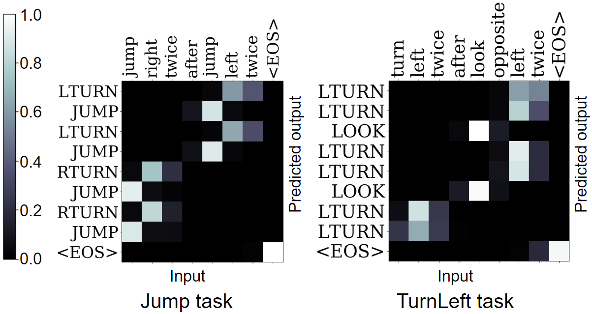
Figure 3: Visualization of attention maps. The figures show that the model solves the problem in a manner similar to humans, identifying the appropriate input to map to each output position. This indicates that the generalizable prior knowledge is successfully encoded in the network.

To investigate whether the proposed method works in the expected way, we visualize the model’s attention maps. These maps indicate whether the sequence-to-sequence model produces correct position sequences.

We visualized these activations for one sample from the Jump task and one from the TurnLeft task (Figure 3). In both figures, the horizontal dimension is the input sequence position, and the vertical dimension is the output position. Each figure is an $m\times n$ matrix, where $m$ and $n$ are output and input lengths, including end-of-sentence symbols. The rows correspond to $m$ attention maps, where the $i$th row corresponds to the attention map for the $i$th output ($i=1,...,m$). The values in each row sum to 1.

We expect that each attention map attends on the corresponding primitive input word. For the output end-of-sentence symbol, we expect that the attention is on the input end-of-sentence symbol. The visualization in both figures align with our expectation. When the model should replicate some input word multiple times, it correctly attends on that word in a manner similar to human understanding. In the Jump example, “jump” appears twice in the input. As expected, the generated attentions are on the second instance for the early part of the output, and on the first instance for the later part of the output. Similarly, the attentions are correct in the TurnLeft example with two words of “left”.

These visualizations demonstrate that the models work in the way we expected, correctly parsing the organization of complex sentences. We have successfully encoded our prior knowledge to the network, and enabled compositional generalization.

4.2 Ablation Study

We conducted an ablation study to find out what factors of the proposed approach contribute to its high performance. The main idea of the proposed approach is to use two representations and corresponding entropy regularization. Also, for autoregressive decoders, the approach does not use the last output rather than feeding it as input for decoding. Based on that, we designed the following ablation experiments.

(A) Use only one representation.

(B) Do not use primitive entropy regularization.

(C) Do not use function entropy regularization.

(D) Both B and C.

(E) Use the last output as input in decoding.

The results are summarized in Table 7. Experiment A shows that the accuracy drops in both tasks, indicating that two representations are important factor in the proposed approach. When there are two representations, we find the following from experiments B, C and D. For Jump task, the accuracy drops in these three experiments, indicating both primitive and function entropy regularization are necessary. For TurnLeft task, the accuracy drops only in D, but not in B or C, indicating at least one of entropy regularization is necessary. The difference between Jump and TurnLeft tasks may be because TurnLeft is relatively easier than the Jump task. Both “turn” and “left” individually appear with other words in training data, but “jump” does not. Experiment E shows that we should not use last output as next input during decoding.

	Experiment	Jump	TurnLeft
A	one rep.	63.4 $\pm$ 36.3	55.7 $\pm$ 31.5
B	no prim reg.	79.8 $\pm$ 11.3	99.9 $\pm$   0.1
C	no func reg.	29.5 $\pm$ 36.3	99.6 $\pm$   1.0
D	both B and C	14.1 $\pm$ 23.2	64.0 $\pm$ 40.0
E	decoder input	68.8 $\pm$ 15.0	50.3 $\pm$ 48.8
	Proposed	98.8 $\pm$   1.4	99.7 $\pm$   0.4

Table 7: Ablation: Test accuracy (mean $\pm$ std %) for SCAN Primitive tasks.

4.3 Influence on Other Tasks

To find whether the proposed method affects other tasks, we conducted experiments on Simple and Length tasks in SCAN dataset. In Simple task, test data follows the same distribution as the training data. In Length task, test commands have longer action sequences than training. Simple task does not require compositional generalization, and Length task requires syntactic generalization, so that they are beyond the scope of this paper. However, we still hope to avoid big performance drop from previous methods. We used the same configuration (Appendix A) as SCAN Primitive tasks. The results in Table 8 confirms that the approach does not significantly reduce performance in other tasks.

Methods	Simple	Length
L&B best overall	99.7	13.8
L&B best	99.8	20.8
RNN +Attn -Dep	100.0 $\pm$ 0.0	11.7 $\pm$ 3.2
GRU +Attn	100.0 $\pm$ 0.0	18.1 $\pm$ 1.1
Ptr-Bahdanau	-	13.4 $\pm$ 0.8
Ptr-Loung	-	16.8 $\pm$ 0.9
Proposed	99.9 $\pm$ 0.0	20.3 $\pm$ 1.1

Table 8: Test accuracy (mean $\pm$ std %) for other SCAN tasks. L&B is from Lake and Baroni (2018). RNN and GRU are best models for each task from Bastings et al. (2018). Ptr-Bahdanau and Ptr-Loung are from Kliegl and Xu (2018). The proposed method does not significantly reduce performance.

5 Related Work

Human-level compositional learning has been an important open challenge Yang et al. (2019), although there is a long history of studying compositionality in neural networks. Classic view Fodor and Pylyshyn (1988); Marcus (1998); Fodor and Lepore (2002) considers conventional neural networks lack systematic compositionality. With the breakthroughs in sequence to sequence neural networks for NLP and other tasks, such as RNN Sutskever et al. (2014), Attention Xu et al. (2015), Pointer Network Vinyals et al. (2015), and Transformer Vaswani et al. (2017), there are more contemporary attempts to encode compositionality in sequence to sequence neural networks.

There has been exploration on compositionality in neural networks for systematic behaviour Wong and Wang (2007); Brakel and Frank (2009), counting ability Rodriguez and Wiles (1998); Weiss et al. (2018) and sensitivity to hierarchical structure Linzen et al. (2016). Recently, many related tasks Lake and Baroni (2018); Loula et al. (2018a); Liška et al. (2018); Bastings et al. (2018); Lake et al. (2019) and methods Bastings et al. (2018); Loula et al. (2018a); Kliegl and Xu (2018); Chang et al. (2018) using a variety of RNN models and attention mechanism have been proposed. These methods make successful generalization when the difference between training and test commands are small.

Our research further enhances the capability of neural networks for compositional generalization with two representations of a sentence and entropy regularization. The proposed approach has shown promising results in various tasks of instruction learning and machine translation.

Compositionality is also important and applicable in multimodal problems, including AI complete tasks like Image Captioning Karpathy and Fei-Fei (2015), Visual Question Answering Antol et al. (2015), Embodied Question Answering Das et al. (2018). These tasks requires compositional understanding of sequences (captions or questions), where our method could help. Compositional understanding could also help enable better transfer over time that could improve continual learning Zenke et al. (2017); Aljundi et al. (2018); Chaudhry et al. (2019) ability of AI models.

6 Conclusions

This work is a fundamental research for encoding compositionality in neural networks. Our approach leverages prior knowledge of compositionality by using two representations, and by reducing entropy in each representation. The experiments demonstrate significant improvements over the conventional methods in five NLP tasks including instruction learning and machine translation. In the SCAN domain, it boosts accuracies from 14.0% to 98.8% in Jump task, and from 92.0% to 99.7% in TurnLeft task. It also beats human performance on a few-shot learning task. To our best knowledge, this is the first time machines beat humans in a few-shot learning task. This breaks the common sense that humans have advantage over machines in learning from few samples. We hope this work opens a path to encourage machines learn quickly and generalize widely like humans do, and to make machines more helpful in various tasks.

Appendix A SCAN Tasks

For the sequence to sequence architecture, we use bidirectional LSTM as encoder, and unidirectional LSTM with attention as decoder. The first and last states of encoder are concatenated as initial state of decoder. The state size is $m=16$ for encoder, and $2m=32$ for decoder. For all SCAN tasks, the primitive embedding size $k_{p}$ and function embedding size $k_{f}$ are both 8. The weight for $L_{2}$ norm regularization $\lambda$ is 0.01, and noise weight $\alpha$ is 1. We use Adam Kingma and Ba (2014) for optimization. We ran 10,000 training steps. Each step has a mini-batch of 64 samples randomly and uniformly selected from training data with replacement. We clip gradient by global norm of 1. Initial learning rate is 0.01 and it exponentially decays by a factor of 0.96 every 100 steps. We use TensorFlow Abadi et al. (2016) for implementation.

SCAN dataset contains four sub datasets. Jump task contains 14,670 training and 7,706 test samples. TurnLeft task contains 21,890 training and 1,208 test samples. Simple task contains 16,728 training and 4,182 test samples. Length task contains 16,990 training and 3,920 test samples. We aim at Jump and TurnLeft tasks in the main experiments. Since Simple task does not require compositional generalization, and Length task requires syntactic generalization, they are beyond the scope of this paper. However, we still evaluate them to show that their performance is not significantly reduced.

Appendix B SCAN Template-matching

We extend experiments to SCAN template-matching task Loula et al. (2018b). There are four tasks in this dataset. In jump around right task, the test set includes all samples containing “jump around right” (1,173 samples), and training set consists of the remaining samples (18,528 samples). In primitive right task, the test set includes all samples containing “Primitive right” (4,476 samples), and the training set consists of the remaining templates (15,225 samples). In primitive opposite right task, the test set includes all samples containing templates in the form “Primitive opposite right” (4,476 samples), and the training set consists of remaining templates (including their conjunctions and quantifications) (15,225 samples). In primitive around right task, the test set includes all samples containing templates in the form “Primitive around right” (4,476 samples), and the training set consists of remaining templates (15,225 samples).

For primitive around right task, we set $m=8,k_{p}=k_{f}=128,\lambda=0.1$, and $\alpha=0.1$. For other tasks, we use the same model configurations as SCAN Jump task.

Appendix C Primitive and Functional Information Exist in One Word

S	$\rightarrow$	V A N
A	$\rightarrow$	C R M $|$ C M R $|$ R C M $|$ R M C $|$ M C R $|$ M R C
V	$\rightarrow$	push $|$ pull $|$ raise $|$ spin
R	$\rightarrow$	small $|$ large
C	$\rightarrow$	yellow $|$ purple $|$ brown $|$ blue $|$ red $|$ gray $|$ green $|$ cyan
M	$\rightarrow$	metal $|$ plastic $|$ rubber
N	$\rightarrow$	sphere $|$ cylinder $|$ cube

Table 9: Commands for grammar in the extended experiment. The material of rubber only appears with other fixed words in training “push small yellow rubber sphere”. However, it appears with other combinations of words in test.

We constructed a dataset with both primitive and functional information contained in one word using the grammar in Table 9. The training data contains 2,560 samples, and test data 1,151 samples. For the proposed approach, we set $m=32,\lambda=0.1,\alpha=0.3$, and we run 5,000 training steps. We keep other configurations the same as SCAN task. For comparison, we use standard LSTM with attention. The hyper parameters are the same as the proposed approach.

Appendix D Few-shot Learning task

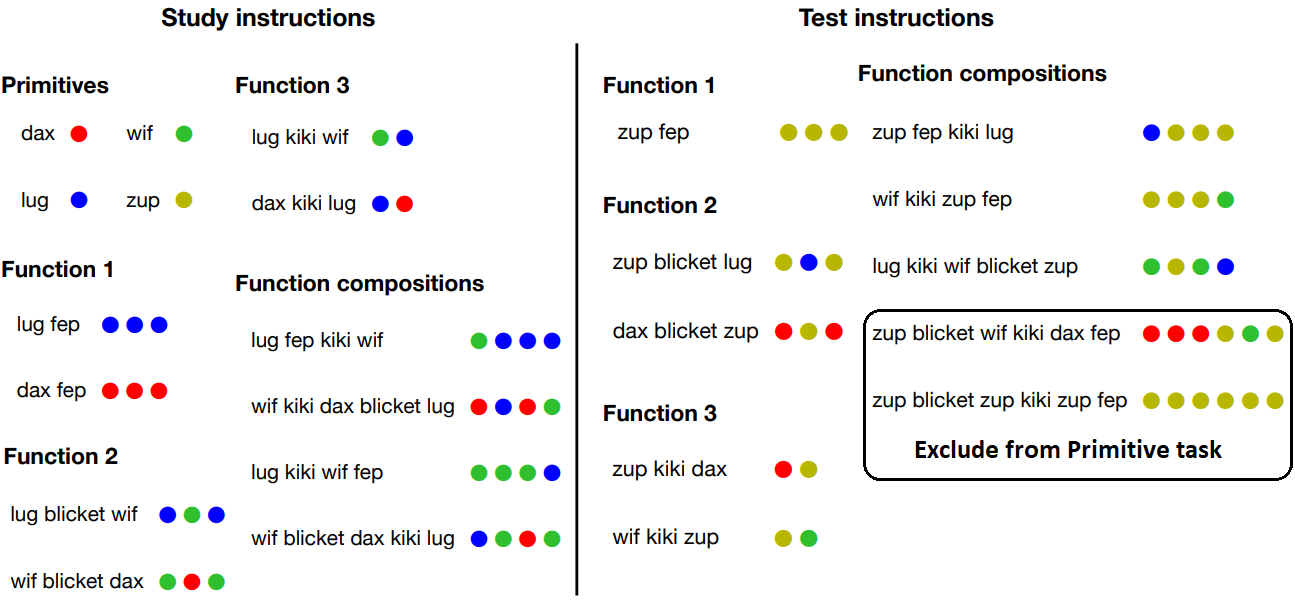
Figure 4: Few-shot instruction learning dataset. Participants learn to produce abstract outputs (colored circles) from instructions in pseudowords. Some pseudowords are primitives corresponding to a single output symbol, while others are function words that process items. A primitive (“zup”) is presented only in isolation during training and is evaluated with other words during test. Participants are expected to learn each function from limited number of examples, and generalize compositionally. This figure is modified from Lake et al. (2019).

For few-shot learning task, we set $k_{p}=k_{f}=16$ and $\lambda=0.1$. We keep other configurations the same as SCAN task.

The dataset Lake et al. (2019) is shown in Figure 4. It contains 14 training and 10 test samples. Among them, 8 test samples correspond to Primitive task. The other 2 test samples requires syntactic generalization which is beyond the scope of this paper.

Appendix E Machine Translation

The experimental setting of machine translation follows Lake and Baroni (2018). The training data contains 10,000 English-French sentence pairs. The sentences are selected to be less than 10 words in length, and starting from English phrases such as “I am”, “he is” and their contractions. The training data also contains 1,000 repetition of sentence pair (“I am daxy”, “je suis daxiste”). Note that “dax” does not appear in the first set of training data. The two sets of training data are mixed and randomized. The test data contains 8 pairs of sentences that contain “daxy” in different patterns from training data, for example (“you are not daxy”, “tu n’es pas daxiste”).

The model configurations are similar to SCAN tasks, except that we set $m=32,k_{p}=k_{f}=32$, $\lambda=1$ and $\alpha=1$ in experiments. The result shows that some predicted outputs differ from the reference, but they are correct translations. Please see Table 10 for details.

Input	Output
you are daxy .	tu es daxiste .
	vous etes daxiste .
you are not daxy .	tu n es pas daxiste .
	vous n etes pas daxiste .
you are very daxy .	tu es tres daxiste .
	vous etes tres daxiste .

Table 10: Test prediction mistakes in machine translation task (normalized). All mistakes are actually correct. Left part is input. Right part is output for reference (upper) and hypothesis (lower).

References

- Abadi et al. (2016) Martín Abadi, Paul Barham, Jianmin Chen, Zhifeng Chen, Andy Davis, Jeffrey Dean, Matthieu Devin, Sanjay Ghemawat, Geoffrey Irving, Michael Isard, et al. 2016. Tensorflow: A system for large-scale machine learning. In 12th USENIX Symposium on Operating Systems Design and Implementation (OSDI 16), pages 265–283.
- Aljundi et al. (2018) Rahaf Aljundi, Francesca Babiloni, Mohamed Elhoseiny, Marcus Rohrbach, and Tinne Tuytelaars. 2018. Memory aware synapses: Learning what (not) to forget. In Proceedings of the European Conference on Computer Vision (ECCV), pages 139–154.
- Antol et al. (2015) Stanislaw Antol, Aishwarya Agrawal, Jiasen Lu, Margaret Mitchell, Dhruv Batra, C Lawrence Zitnick, and Devi Parikh. 2015. Vqa: Visual question answering. In Proceedings of the IEEE international conference on computer vision, pages 2425–2433.
- Bastings et al. (2018) Joost Bastings, Marco Baroni, Jason Weston, Kyunghyun Cho, and Douwe Kiela. 2018. Jump to better conclusions: SCAN both left and right. In Proceedings of the 2018 EMNLP Workshop BlackboxNLP: Analyzing and Interpreting Neural Networks for NLP, pages 47–55, Brussels, Belgium. Association for Computational Linguistics.
- Brakel and Frank (2009) Philémon Brakel and Stefan Frank. 2009. Strong systematicity in sentence processing by simple recurrent networks. In 31th Annual Conference of the Cognitive Science Society (COGSCI-2009), pages 1599–1604. Cognitive Science Society.
- Calvo and Symons (2014) Paco Calvo and John Symons. 2014. The Architecture of Cognition: Rethinking Fodor and Pylyshyn’s Systematicity Challenge. MIT Press.
- Chang et al. (2018) Michael B Chang, Abhishek Gupta, Sergey Levine, and Thomas L Griffiths. 2018. Automatically composing representation transformations as a means for generalization. arXiv preprint arXiv:1807.04640.
- Chaudhry et al. (2019) Arslan Chaudhry, Marc’Aurelio Ranzato, Marcus Rohrbach, and Mohamed Elhoseiny. 2019. Efficient lifelong learning with a-gem. In ICLR.
- Chomsky (1957) Noam Chomsky. 1957. Syntactic structures. Walter de Gruyter.
- Das et al. (2018) Abhishek Das, Samyak Datta, Georgia Gkioxari, Stefan Lee, Devi Parikh, and Dhruv Batra. 2018. Embodied question answering. In Proceedings of the IEEE Conference on Computer Vision and Pattern Recognition Workshops, pages 2054–2063.
- Fodor and Lepore (2002) Jerry A Fodor and Ernest Lepore. 2002. The compositionality papers. Oxford University Press.
- Fodor and Pylyshyn (1988) Jerry A Fodor and Zenon W Pylyshyn. 1988. Connectionism and cognitive architecture: A critical analysis. Cognition, 28(1-2):3–71.
- He et al. (2016) K. He, X. Zhang, S. Ren, and J. Sun. 2016. Deep residual learning for image recognition. In CVPR.
- Karpathy and Fei-Fei (2015) Andrej Karpathy and Li Fei-Fei. 2015. Deep visual-semantic alignments for generating image descriptions. In Proceedings of the IEEE conference on computer vision and pattern recognition, pages 3128–3137.
- Kingma and Ba (2014) Diederik P Kingma and Jimmy Ba. 2014. Adam: A method for stochastic optimization. arXiv preprint arXiv:1412.6980.
- Kliegl and Xu (2018) Markus Kliegl and Wei Xu. 2018. More systematic than claimed: Insights on the scan tasks. OpenReview.
- Krizhevsky et al. (2012) A. Krizhevsky, I. Sutskever, and G.E. Hinton. 2012. Imagenet classification with deep convolutional neural networks. In NIPS.
- Lake and Baroni (2018) Brenden Lake and Marco Baroni. 2018. Generalization without systematicity: On the compositional skills of sequence-to-sequence recurrent networks. In International Conference on Machine Learning, pages 2879–2888.
- Lake et al. (2019) Brenden M Lake, Tal Linzen, and Marco Baroni. 2019. Human few-shot learning of compositional instructions. arXiv preprint arXiv:1901.04587.
- Lake et al. (2017) Brenden M Lake, Tomer D Ullman, Joshua B Tenenbaum, and Samuel J Gershman. 2017. Building machines that learn and think like people. Behavioral and Brain Sciences, 40.
- LeCun et al. (2015) Yann LeCun, Yoshua Bengio, and Geoffrey Hinton. 2015. Deep learning. nature, 521(7553):436.
- Linzen et al. (2016) Tal Linzen, Emmanuel Dupoux, and Yoav Goldberg. 2016. Assessing the ability of lstms to learn syntax-sensitive dependencies. Transactions of the Association for Computational Linguistics, 4:521–535.
- Liška et al. (2018) Adam Liška, Germán Kruszewski, and Marco Baroni. 2018. Memorize or generalize? searching for a compositional rnn in a haystack. arXiv preprint arXiv:1802.06467.
- Loula et al. (2018a) Joao Loula, Marco Baroni, and Brenden M Lake. 2018a. Rearranging the familiar: Testing compositional generalization in recurrent networks. arXiv preprint arXiv:1807.07545.
- Loula et al. (2018b) Joao Loula, Marco Baroni, Brenden M, and Linzen. 2018b. Rearrange the familiar: testing compositional generalization in recurrent networks. arXiv preprint arXiv:1807.07545.
- Marcus (1998) Gary F Marcus. 1998. Rethinking eliminative connectionism. Cognitive psychology, 37(3):243–282.
- Marcus (2003) Gary F Marcus. 2003. The algebraic mind: Integrating connectionism and cognitive science. MIT press.
- Minsky (1986) Marvin Minsky. 1986. Society of mind. Simon and Schuster.
- Montague (1970) Richard Montague. 1970. Universal grammar. Theoria, 36(3):373–398.
- Rodriguez and Wiles (1998) Paul Rodriguez and Janet Wiles. 1998. Recurrent neural networks can learn to implement symbol-sensitive counting. In Advances in Neural Information Processing Systems, pages 87–93.
- Sutskever et al. (2014) Ilya Sutskever, Oriol Vinyals, and Quoc V Le. 2014. Sequence to sequence learning with neural networks. In Advances in neural information processing systems, pages 3104–3112.
- Vaswani et al. (2017) Ashish Vaswani, Noam Shazeer, Niki Parmar, Jakob Uszkoreit, Llion Jones, Aidan N Gomez, Łukasz Kaiser, and Illia Polosukhin. 2017. Attention is all you need. In Advances in Neural Information Processing Systems, pages 5998–6008.
- Vinyals et al. (2015) Oriol Vinyals, Meire Fortunato, and Navdeep Jaitly. 2015. Pointer networks. In Advances in Neural Information Processing Systems, pages 2692–2700.
- Weiss et al. (2018) Gail Weiss, Yoav Goldberg, and Eran Yahav. 2018. On the practical computational power of finite precision rnns for language recognition. arXiv preprint arXiv:1805.04908.
- Wong and Wang (2007) Francis CK Wong and William SY Wang. 2007. Generalisation towards combinatorial productivity in language acquisition by simple recurrent networks. In 2007 International Conference on Integration of Knowledge Intensive Multi-Agent Systems, pages 139–144. IEEE.
- Wu and et al (2016) Y. Wu and et al. 2016. Google’s neural machine translation system: Bridging the gap between human and machine translation. In arXiv:1609.08144.
- Xu et al. (2015) Kelvin Xu, Jimmy Ba, Ryan Kiros, Kyunghyun Cho, Aaron Courville, Ruslan Salakhudinov, Rich Zemel, and Yoshua Bengio. 2015. Show, attend and tell: Neural image caption generation with visual attention. In International conference on machine learning, pages 2048–2057.
- Yang et al. (2019) Guangyu Robert Yang, Madhura R Joglekar, H Francis Song, William T Newsome, and Xiao-Jing Wang. 2019. Task representations in neural networks trained to perform many cognitive tasks. Nature neuroscience, page 1.
- Yu and Deng (2012) D. Yu and L. Deng. 2012. Automatic Speech Recognition. Springer.
- Zenke et al. (2017) Friedemann Zenke, Ben Poole, and Surya Ganguli. 2017. Continual learning through synaptic intelligence. In Proceedings of the 34th International Conference on Machine Learning-Volume 70, pages 3987–3995. JMLR. org.