BiLQ: An Iterative Method for Nonsymmetric Linear Systems with a Quasi-Minimum Error Property

Abstract

We introduce an iterative method named BiLQ for solving general square linear systems $Ax=b$ based on the Lanczos biorthogonalization process defined by least-norm subproblems, and that is a natural companion to BiCG and Qmr. Whereas the BiCG (Fletcher, 1976), Cgs (Sonneveld, 1989) and BiCGStab (van der Vorst, 1992) iterates may not exist when the tridiagonal projection of $A$ is singular, BiLQ is reliable on compatible systems even if A is ill-conditioned or rank deficient. As in the symmetric case, the BiCG residual is often smaller than the BiLQ residual and, when the BiCG iterate exists, an inexpensive transfer from the BiLQ iterate is possible. Although the Euclidean norm of the BiLQ error is usually not monotonic, it is monotonic in a different norm that depends on the Lanczos vectors. We establish a similar property for the Qmr (Freund and Nachtigal, 1991) residual. BiLQ combines with Qmr to take advantage of two initial vectors and solve a system and an adjoint system simultaneously at a cost similar to that of applying either method. We derive an analogous combination of Usymlq and Usymqr based on the orthogonal tridiagonalization process (Saunders et al., 1988). The resulting combinations, named BiLQR and TriLQR, may be used to estimate integral functionals involving the solution of a primal and an adjoint system. We compare BiLQR and TriLQR with Minres-qlp on a related augmented system, which performs a comparable amount of work and requires comparable storage. In our experiments, BiLQR terminates earlier than TriLQR and Minres-qlp in terms of residual and error of the primal and adjoint systems.

15A06, 65F10, 65F25, 65F50, 93E24 90C06

1 Introduction

We consider the square consistent linear system

(1) $$Ax=b,$$

where $A\in\mathds{R}^{n\times n}$ can be nonsymmetric, is either large and sparse, or is only available as a linear operator, i.e., via operator-vector products. We assume that $A$ is nonsingular. Systems such as (1) arise in the discretization of partial differential equations (PDEs) in numerous applications, including compressible turbulent fluid flow (Chisholm and Zingg, 2009), and in circuit simulation (Davis and Natarajan, 2012). We consider Krylov subspace methods and are interested in generating iterates with guarantees as to the decrease of the error $x_{k}-x_{\star}$ in a certain norm, where $x_{\star}$ is the solution of (1).

The foundation of Krylov methods is a basis-generation process upon which three methods may be developped: one computing the minimum-norm solution of an under-determined system, one solving a square system and imposing a Galerkin condition, and one solving an over-determined system in the least-squares sense. These methods may be implemented with the help of a LQ, LU or QR factorization of a related operator, respectively.

In this paper, we develop an iterative method named BiLQ of the first type based on the Lanczos (1950) biorthogonalization process. Together with BiCG (Fletcher, 1976) and Qmr (Freund and Nachtigal, 1991), BiLQ completes the family of methods based on the biorthogonalization process. We begin by stating the defining properties of BiLQ, describing its implementation in detail, and illustrating its behavior on numerical examples side by side with BiCG and Qmr.

In a second stage, we exploit the fact that the biorthogonalization process requires two initial vectors to develop a combination of BiLQ and Qmr that solves (1) together with a dual system

(2) $$A^{T}t=c$$

simultaneously at a cost comparable to that of applying BiLQ or Qmr only to solve one of those systems. The resulting combination is named BiLQR and is employed to illustrate the computation of superconvergent estimates of integral functionals arising in certain PDE problems.

We note that a similar approach may be developed for the Saunders et al. (1988) orthogonal tridiagonalization process, which also requires two initial vectors, by combining Usymlq and Usymqr. The resulting combination is named TriLQR.

Finally, we compare BiLQR and TriLQR with Minres-qlp on a related augmented system to solve both (1) and (2) simultaneously. In our experiments, BiLQR terminates earlier than TriLQR and Minres-qlp in terms of residual and error of the primal and adjoint systems.

Our Julia (Bezanson et al., 2017) implementation of BiLQ, Qmr, Usymlq, Usymqr, BiLQR, TriLQR, and Minres-qlp are available from github.com/JuliaSmoothOptimizers/Krylov.jl. Thanks to multiple dispatch, a language feature allowing automatic compilation of variants of each method corresponding to inputs expressed in various floating-point systems, our implementations run in any floating-point precision supported.

Related Research

Paige and Saunders (1975) develop one of the best-known minimum error methods, Symmlq, based on the symmetric Lanczos process. Symmlq inspires Estrin et al. (2019a, b) to develop Lslq and Lnlq for rectangular problems based on the Golub and Kahan (1965) process. Lslq and Lnlq are equivalent to Symmlq applied to the normal equations and normal equations of the second kind, respectively.

Saunders et al. (1988) define Usymlq for square consistent systems based on the orthogonal tridiagonalization process. Usymlq is based on a subproblem similar to that of Symmlq, and coincides with Symmlq in the symmetric case. Its companion method, Usymqr, is similar in spirit to Minres. Buttari et al. (2019) combine both into a method named Usymlqr designed to solve symmetric saddle-point systems with general right-hand side, and inspire the developement of BiLQR and TriLQR in the present paper.

Weiss (1994) decribes two types of error-minimizing Krylov methods for square $A$; one based on a process applied to $A^{T}A$, and one to $A^{T}$. Our approach is to apply the biorthogonalization process directly to $A$. We defer a numerical stability analysis to future work, but note that Paige et al. (2014) study the augmented stability of the biorthogonalization process. In this sense, we make the implicit assumption that computations are carried out in exact arithmetic. This assumption prompted us to develop our implementations so that they can be applied in any supported floating-point arithmetic.

The simultaneous solution of a system and an adjoint system has attracted attention in the past. Notably, Lu and Darmofal (2003) devise a variant of Qmr to solve both systems at once at a cost approximately equal to that of Qmr applied to one of the systems but with an increase in storage requirements. Golub et al. (2008) follow a similar approach and use a variant of Usymqr to solve both (1) and (2). An advantage of Usymqr is to produce monotonic residuals in the Euclidean norm for both systems. We illustrate in Table 2 that our methods are cheaper and have smaller storage requirements than those of Lu and Darmofal (2003) and Golub et al. (2008) though residuals are not monotonic in the Euclidean norm.

Notation

Matrices and vectors are denoted by capital and lowercase Latin letters, respectively, and scalars by Greek letters. An exception is made for Givens cosines and sines $(c,s)$ that compose reflections. For a vector v, $\|v\|$ denotes the Euclidean norm of $v$, and for symmetric and positive-definite $N$, the $N$-norm of $v$ is $\|v\|_{N}^{2}=v^{T}Nv$. For a matrix $M$, $\|M\|_{F}$ denotes the Frobenius norm of $M$. The vector $e_{i}$ is the $i$-th column of an identity matrix of size dictated by the context. Vectors and scalars decorated by a bar will be updated at the next iteration. For $j=2,\dots,k$, we use the compact representation

$$Q_{j-1,j}=\hbox{}\vbox{\kern 0.86108pt\hbox{$\kern 0.0pt\kern 2.5pt\kern-5.0pt\left[\kern 0.0pt\kern-2.5pt\kern-5.55557pt\vbox{\kern-0.86108pt\vbox{\vbox{ \halign{\kern\arraycolsep\hfil\@arstrut$\kbcolstyle#$\hfil\kern\arraycolsep& \kern\arraycolsep\hfil$\@kbrowstyle#$\ifkbalignright\relax\else\hfil\fi\kern\arraycolsep&& \kern\arraycolsep\hfil$\@kbrowstyle#$\ifkbalignright\relax\else\hfil\fi\kern\arraycolsep\cr 5.0pt\hfil\@arstrut$\scriptstyle$\hfil\kern 5.0pt&5.0pt\hfil$\scriptstyle j-1$\hfil\kern 5.0pt&5.0pt\hfil$\scriptstyle j\\$\hfil\kern 5.0pt&5.0pt\hfil$\scriptstyle c_{j}$\hfil\kern 5.0pt&5.0pt\hfil$\scriptstyle\phantom{-}s_{j}\\$\hfil\kern 5.0pt&5.0pt\hfil$\scriptstyle s_{j}$\hfil\kern 5.0pt&5.0pt\hfil$\scriptstyle-c_{j}$\hfil\kern 5.0pt\crcr}}}}\right]$}}:=\begin{bmatrix}I_{j-2}&&&\\ &c_{j}&\phantom{-}s_{j}&\\ &s_{j}&-c_{j}&\\ &&&I_{k-j}\end{bmatrix},$$

for orthogonal reflections, where $s_{j}^{2}+c_{j}^{2}=1$, where border indices indicate row and column numbers, and where $I_{k}$ represents the $k$$\times$$k$ identity operator. We abuse the notation $\bar{z}_{k}=(z_{k-1},~{}\bar{\zeta}_{k})$ to represent the column vector $\begin{bmatrix}z_{k-1}^{T}&\bar{\zeta}_{k}\end{bmatrix}^{T}$.

2 Derivation of BiLQ

2.1 The Lanczos Biorthogonalization Process

The Lanczos biorthogonalization process generates sequences of vectors $\{v_{k}\}$ and $\{u_{k}\}$ such that $v_{i}^{T}u_{j}=\delta_{ij}$ in exact arithmetic for as long as the process does not break down. The process is summarized as Algorithm 1.

Algorithm 1 Lanczos Biorthogonalization Process

1:$A$, $b$, $c$

2:$v_{0}=0$, $u_{0}=0$

3:$\beta_{1}v_{1}=b$, $\gamma_{1}u_{1}=c$ $(\beta_{1},\gamma_{1})$ so that $v_{1}^{T}u_{1}=1$

4:for $k$ = 1, 2, $\dots$ do

5:     $q=Av_{k}-\gamma_{k}v_{k-1}$, $\alpha_{k}=u_{k}^{T}q$

6:     $p=A^{T}u_{k}-\beta_{k}u_{k-1}$

7:     $\beta_{k+1}v_{k+1}=q-\alpha_{k}v_{k}$ $(\beta_{k+1},\gamma_{k+1})$ so that $v_{k+1}^{T}u_{k+1}=1$

8:     $\gamma_{k+1}u_{k+1}=p-\alpha_{k}u_{k}$

9:end for

We denote $V_{k}=\begin{bmatrix}v_{1}&\dots&v_{k}\end{bmatrix}$ and $U_{k}=\begin{bmatrix}u_{1}&\dots&u_{k}\end{bmatrix}$. Without loss of generality, we choose the scaling factors $\beta_{k}$ and $\gamma_{k}$ so that $v_{k}^{T}u_{k}=1$ for all $k\geq 1$, i.e., $V_{k}^{T}U_{k}=I_{k}$. After $k$ iterations, the situation may be summarized as

(3a) $$AV_{k} =V_{k}T_{k}~{}+\beta_{k+1}v_{k+1}e_{k}^{T}=V_{k+1}T_{k+1,k}$$

(3b) $$A^{T}U_{k} =U_{k}T_{k}^{T}+\gamma_{k+1}u_{k+1}e_{k}^{T}=U_{k+1}T_{k,k+1}^{T},$$

where

$$T_{k}=\begin{bmatrix}\alpha_{1}&\gamma_{2}&&\\ \beta_{2}&\alpha_{2}&\ddots&\\ &\ddots&\ddots&\gamma_{k}\\ &&\beta_{k}&\alpha_{k}\end{bmatrix},~{}T_{k,k+1}=\begin{bmatrix}T_{k}&\gamma_{k+1}e_{k}\end{bmatrix},~{}T_{k+1,k}=\begin{bmatrix}T_{k}\\ \beta_{k+1}e_{k}^{T}\end{bmatrix}.$$

The columns of $V_{k}$ and $U_{k}$ form a basis for $\mathcal{K}_{k}:=\mathop{\mathrm{Span}}\{b,Ab,\cdots,A^{k-1}b\}$ and $\mathcal{L}_{k}:=\mathop{\mathrm{Span}}\{c,A^{T}c,\cdots,(A^{T})^{k-1}c\}$, respectively. Though $V_{k}$ cannot be expected to be orthogonal to $U_{k}$ in inexact arithmetic, and therefore $U_{k}^{T}AV_{k}=T_{k}$ cannot be expected to hold, (3) usually holds to within machine precision.

2.2 Definition of BiLQ

By definition, BiLQ generates an approximation $x^{\textup{\tiny L}}_{k}$ to a solution of (1) of the form $x^{\textup{\tiny L}}_{k}=V_{k}y^{\textup{\tiny L}}_{k}$, where $y^{\textup{\tiny L}}_{k}\in\mathds{R}^{k}$ solves

(4) $$\mathop{\textup{minimize}}_{y}\ \|y\|\quad\mathop{\textup{subject to}}\ T_{k-1,k}y=\beta_{1}e_{1}.$$

By contrast, BiCG (Fletcher, 1976) generates $x^{\textup{\tiny C}}_{k}=V_{k}y^{\textup{\tiny C}}_{k}$ where $y^{\textup{\tiny C}}_{k}\in\mathds{R}^{k}$ solves

(5) $$T_{k}y=\beta_{1}e_{1},$$

and Qmr (Freund and Nachtigal, 1991) generates $x^{\textup{\tiny Q}}_{k}=V_{k}y^{\textup{\tiny Q}}_{k}$ where $y^{\textup{\tiny Q}}_{k}\in\mathds{R}^{k}$ solves

(6) $$\mathop{\textup{minimize}}_{y}\ \|T_{k+1,k}y-\beta_{1}e_{1}\|.$$

When A is symmetric and $b=c$, Algorithm 1 coincides with the symmetric Lanczos process and the three above methods are equivalent to Symmlq (Paige and Saunders, 1975), Cg (Hestenes and Stiefel, 1952), and Minres (Paige and Saunders, 1975), respectively.

2.3 An LQ factorization

We determine $y^{\textup{\tiny L}}_{k}$ solution to (4) via the LQ factorization of $T_{k-1,k}$, which we obtain from the LQ factorization

(7a) $$T_{k} =\bar{L}_{k}Q_{k},\text{ where}$$

(7b) $$\overline{L}_{k} =\begin{bmatrix}\delta_{1}&&&&&\\ \lambda_{1}&\delta_{2}&&&&\\ \varepsilon_{1}&\lambda_{2}&\delta_{3}&&&\\ &\ddots&\ddots&\ddots&&\\ &&\varepsilon_{k-3}&\lambda_{k-2}&\delta_{k-1}&\\ &&&\varepsilon_{k-2}&\lambda_{k-1}&\bar{\delta}_{k}\end{bmatrix}=\begin{bmatrix}L_{k-1}&0\\ \varepsilon_{k-2}e^{T}_{k-2}+\lambda_{k-1}e^{T}_{k-1}&\bar{\delta}_{k}\end{bmatrix},$$

and $Q_{k}^{T}=Q_{1,2}Q_{2,3}\cdots Q_{k-1,k}$ is orthogonal and defined as a product of Givens reflections. Indeed, the above yields the LQ factorization

(8) $$T_{k-1,k}=\begin{bmatrix}L_{k-1}&0\end{bmatrix}Q_{k}.$$

If we initialize $\bar{\delta}_{1}:=\alpha_{1}$, $\bar{\lambda}_{1}:=\beta_{2}$, $c_{1}=-1$, and $s_{1}=0$, individual factorization steps may be represented as an application of $Q_{k-2,k-1}$ to $T_{k}Q_{k-2}^{T}$:

$$\hbox{}\vbox{\kern 0.86108pt\hbox{$\kern 0.0pt\kern 2.5pt\kern-5.0pt\left[\kern 0.0pt\kern-2.5pt\kern-5.55557pt\vbox{\kern-0.86108pt\vbox{\vbox{ \halign{\kern\arraycolsep\hfil\@arstrut$\kbcolstyle#$\hfil\kern\arraycolsep& \kern\arraycolsep\hfil$\@kbrowstyle#$\ifkbalignright\relax\else\hfil\fi\kern\arraycolsep&& \kern\arraycolsep\hfil$\@kbrowstyle#$\ifkbalignright\relax\else\hfil\fi\kern\arraycolsep\cr 5.0pt\hfil\@arstrut$\scriptstyle$\hfil\kern 5.0pt&5.0pt\hfil$\scriptstyle k-2$\hfil\kern 5.0pt&5.0pt\hfil$\scriptstyle k-1$\hfil\kern 5.0pt&5.0pt\hfil$\scriptstyle k\\k-2$\hfil\kern 5.0pt&5.0pt\hfil$\scriptstyle\bar{\delta}_{k-2}$\hfil\kern 5.0pt&5.0pt\hfil$\scriptstyle\gamma_{k-1}$\hfil\kern 5.0pt&5.0pt\hfil$\scriptstyle\\k-1$\hfil\kern 5.0pt&5.0pt\hfil$\scriptstyle\bar{\lambda}_{k-2}$\hfil\kern 5.0pt&5.0pt\hfil$\scriptstyle\alpha_{k-1}$\hfil\kern 5.0pt&5.0pt\hfil$\scriptstyle\gamma_{k}\\k$\hfil\kern 5.0pt&5.0pt\hfil$\scriptstyle$\hfil\kern 5.0pt&5.0pt\hfil$\scriptstyle\beta_{k}$\hfil\kern 5.0pt&5.0pt\hfil$\scriptstyle\alpha_{k}$\hfil\kern 5.0pt\crcr}}}}\right]$}}\hbox{}\vbox{\kern 0.86108pt\hbox{$\kern 0.0pt\kern 2.5pt\kern-5.0pt\left[\kern 0.0pt\kern-2.5pt\kern-5.55557pt\vbox{\kern-0.86108pt\vbox{\vbox{ \halign{\kern\arraycolsep\hfil\@arstrut$\kbcolstyle#$\hfil\kern\arraycolsep& \kern\arraycolsep\hfil$\@kbrowstyle#$\ifkbalignright\relax\else\hfil\fi\kern\arraycolsep&& \kern\arraycolsep\hfil$\@kbrowstyle#$\ifkbalignright\relax\else\hfil\fi\kern\arraycolsep\cr 5.0pt\hfil\@arstrut$\scriptstyle$\hfil\kern 5.0pt&5.0pt\hfil$\scriptstyle k-2$\hfil\kern 5.0pt&5.0pt\hfil$\scriptstyle k-1$\hfil\kern 5.0pt&5.0pt\hfil$\scriptstyle k\\$\hfil\kern 5.0pt&5.0pt\hfil$\scriptstyle c_{k-1}$\hfil\kern 5.0pt&5.0pt\hfil$\scriptstyle\phantom{-}s_{k-1}$\hfil\kern 5.0pt&5.0pt\hfil$\scriptstyle\\$\hfil\kern 5.0pt&5.0pt\hfil$\scriptstyle s_{k-1}$\hfil\kern 5.0pt&5.0pt\hfil$\scriptstyle-c_{k-1}$\hfil\kern 5.0pt&5.0pt\hfil$\scriptstyle\\$\hfil\kern 5.0pt&5.0pt\hfil$\scriptstyle$\hfil\kern 5.0pt&5.0pt\hfil$\scriptstyle$\hfil\kern 5.0pt&5.0pt\hfil$\scriptstyle 1$\hfil\kern 5.0pt\crcr}}}}\right]$}}=\hbox{}\vbox{\kern 0.86108pt\hbox{$\kern 0.0pt\kern 2.5pt\kern-5.0pt\left[\kern 0.0pt\kern-2.5pt\kern-5.55557pt\vbox{\kern-0.86108pt\vbox{\vbox{ \halign{\kern\arraycolsep\hfil\@arstrut$\kbcolstyle#$\hfil\kern\arraycolsep& \kern\arraycolsep\hfil$\@kbrowstyle#$\ifkbalignright\relax\else\hfil\fi\kern\arraycolsep&& \kern\arraycolsep\hfil$\@kbrowstyle#$\ifkbalignright\relax\else\hfil\fi\kern\arraycolsep\cr 5.0pt\hfil\@arstrut$\scriptstyle$\hfil\kern 5.0pt&5.0pt\hfil$\scriptstyle k-2$\hfil\kern 5.0pt&5.0pt\hfil$\scriptstyle k-1$\hfil\kern 5.0pt&5.0pt\hfil$\scriptstyle k\\$\hfil\kern 5.0pt&5.0pt\hfil$\scriptstyle\delta_{k-2}$\hfil\kern 5.0pt&5.0pt\hfil$\scriptstyle 0$\hfil\kern 5.0pt&5.0pt\hfil$\scriptstyle\\$\hfil\kern 5.0pt&5.0pt\hfil$\scriptstyle\lambda_{k-2}$\hfil\kern 5.0pt&5.0pt\hfil$\scriptstyle\bar{\delta}_{k-1}$\hfil\kern 5.0pt&5.0pt\hfil$\scriptstyle\gamma_{k}\\$\hfil\kern 5.0pt&5.0pt\hfil$\scriptstyle\varepsilon_{k-2}$\hfil\kern 5.0pt&5.0pt\hfil$\scriptstyle\bar{\lambda}_{k-1}$\hfil\kern 5.0pt&5.0pt\hfil$\scriptstyle\alpha_{k}$\hfil\kern 5.0pt\crcr}}}}\right]$}},$$

followed by an application of $Q_{k-1,k}$ to the result:

$$\hbox{}\vbox{\kern 0.86108pt\hbox{$\kern 0.0pt\kern 2.5pt\kern-5.0pt\left[\kern 0.0pt\kern-2.5pt\kern-5.55557pt\vbox{\kern-0.86108pt\vbox{\vbox{ \halign{\kern\arraycolsep\hfil\@arstrut$\kbcolstyle#$\hfil\kern\arraycolsep& \kern\arraycolsep\hfil$\@kbrowstyle#$\ifkbalignright\relax\else\hfil\fi\kern\arraycolsep&& \kern\arraycolsep\hfil$\@kbrowstyle#$\ifkbalignright\relax\else\hfil\fi\kern\arraycolsep\cr 5.0pt\hfil\@arstrut$\scriptstyle$\hfil\kern 5.0pt&5.0pt\hfil$\scriptstyle k-2$\hfil\kern 5.0pt&5.0pt\hfil$\scriptstyle k-1$\hfil\kern 5.0pt&5.0pt\hfil$\scriptstyle k\\k-2$\hfil\kern 5.0pt&5.0pt\hfil$\scriptstyle\delta_{k-2}$\hfil\kern 5.0pt&5.0pt\hfil$\scriptstyle$\hfil\kern 5.0pt&5.0pt\hfil$\scriptstyle\\k-1$\hfil\kern 5.0pt&5.0pt\hfil$\scriptstyle\lambda_{k-2}$\hfil\kern 5.0pt&5.0pt\hfil$\scriptstyle\bar{\delta}_{k-1}$\hfil\kern 5.0pt&5.0pt\hfil$\scriptstyle\gamma_{k}\\k$\hfil\kern 5.0pt&5.0pt\hfil$\scriptstyle\varepsilon_{k-2}$\hfil\kern 5.0pt&5.0pt\hfil$\scriptstyle\bar{\lambda}_{k-1}$\hfil\kern 5.0pt&5.0pt\hfil$\scriptstyle\alpha_{k}$\hfil\kern 5.0pt\crcr}}}}\right]$}}\hbox{}\vbox{\kern 0.86108pt\hbox{$\kern 0.0pt\kern 2.5pt\kern-5.0pt\left[\kern 0.0pt\kern-2.5pt\kern-5.55557pt\vbox{\kern-0.86108pt\vbox{\vbox{ \halign{\kern\arraycolsep\hfil\@arstrut$\kbcolstyle#$\hfil\kern\arraycolsep& \kern\arraycolsep\hfil$\@kbrowstyle#$\ifkbalignright\relax\else\hfil\fi\kern\arraycolsep&& \kern\arraycolsep\hfil$\@kbrowstyle#$\ifkbalignright\relax\else\hfil\fi\kern\arraycolsep\cr 5.0pt\hfil\@arstrut$\scriptstyle$\hfil\kern 5.0pt&5.0pt\hfil$\scriptstyle k-2$\hfil\kern 5.0pt&5.0pt\hfil$\scriptstyle k-1$\hfil\kern 5.0pt&5.0pt\hfil$\scriptstyle k\\$\hfil\kern 5.0pt&5.0pt\hfil$\scriptstyle 1$\hfil\kern 5.0pt&5.0pt\hfil$\scriptstyle$\hfil\kern 5.0pt&5.0pt\hfil$\scriptstyle\\$\hfil\kern 5.0pt&5.0pt\hfil$\scriptstyle$\hfil\kern 5.0pt&5.0pt\hfil$\scriptstyle c_{k}$\hfil\kern 5.0pt&5.0pt\hfil$\scriptstyle\phantom{-}s_{k}\\$\hfil\kern 5.0pt&5.0pt\hfil$\scriptstyle$\hfil\kern 5.0pt&5.0pt\hfil$\scriptstyle s_{k}$\hfil\kern 5.0pt&5.0pt\hfil$\scriptstyle-c_{k}$\hfil\kern 5.0pt\crcr}}}}\right]$}}=\hbox{}\vbox{\kern 0.86108pt\hbox{$\kern 0.0pt\kern 2.5pt\kern-5.0pt\left[\kern 0.0pt\kern-2.5pt\kern-5.55557pt\vbox{\kern-0.86108pt\vbox{\vbox{ \halign{\kern\arraycolsep\hfil\@arstrut$\kbcolstyle#$\hfil\kern\arraycolsep& \kern\arraycolsep\hfil$\@kbrowstyle#$\ifkbalignright\relax\else\hfil\fi\kern\arraycolsep&& \kern\arraycolsep\hfil$\@kbrowstyle#$\ifkbalignright\relax\else\hfil\fi\kern\arraycolsep\cr 5.0pt\hfil\@arstrut$\scriptstyle$\hfil\kern 5.0pt&5.0pt\hfil$\scriptstyle k-2$\hfil\kern 5.0pt&5.0pt\hfil$\scriptstyle k-1$\hfil\kern 5.0pt&5.0pt\hfil$\scriptstyle k\\$\hfil\kern 5.0pt&5.0pt\hfil$\scriptstyle\delta_{k-2}$\hfil\kern 5.0pt&5.0pt\hfil$\scriptstyle$\hfil\kern 5.0pt&5.0pt\hfil$\scriptstyle\\$\hfil\kern 5.0pt&5.0pt\hfil$\scriptstyle\lambda_{k-2}$\hfil\kern 5.0pt&5.0pt\hfil$\scriptstyle\delta_{k-1}$\hfil\kern 5.0pt&5.0pt\hfil$\scriptstyle\\$\hfil\kern 5.0pt&5.0pt\hfil$\scriptstyle\varepsilon_{k-2}$\hfil\kern 5.0pt&5.0pt\hfil$\scriptstyle\lambda_{k-1}$\hfil\kern 5.0pt&5.0pt\hfil$\scriptstyle\bar{\delta}_{k}$\hfil\kern 5.0pt\crcr}}}}\right]$}}.$$

The reflection $Q_{k-1,k}$ is designed to zero out $\gamma_{k}$ on the superdiagonal of $T_{k}$ and affects three rows and two colums. It is defined by

(9) $$\delta_{k-1}=\sqrt{\bar{\delta}_{k-1}^{2}+\gamma_{k}^{2}},\quad c_{k}=\bar{\delta}_{k-1}/\delta_{k-1},\quad s_{k}=\gamma_{k}/\delta_{k-1},$$

and yields the recursion

(10a) $$\varepsilon_{k-2} =s_{k-1}\beta_{k},\quad k \geq 3,$$

(10b) $$\bar{\lambda}_{k-1} =-c_{k-1}\beta_{k},\quad k \geq 3,$$

(10c) $$\lambda_{k-1} =c_{k}\bar{\lambda}_{k-1}+s_{k}\alpha_{k},\quad k \geq 2,$$

(10d) $$\bar{\delta}_{k} =s_{k}\bar{\lambda}_{k-1}-c_{k}\alpha_{k},\quad k \geq 2.$$

2.4 Definition and update of the BiLQ and BiCG iterates

In order to compute $y_{k}^{\textup{\tiny L}}$ solution of (4) using (8), we solve $\begin{bmatrix}L_{k-1}&0\end{bmatrix}Q_{k}y_{k}^{\textup{\tiny L}}=\beta_{1}e_{1}$. If $z_{k-1}:=(\zeta_{1},\dots,\zeta_{k-1})$ is defined so that $L_{k-1}z_{k-1}=\beta_{1}e_{1}$, then the minimum-norm solution of (4) is $y_{k}^{\textup{\tiny L}}=Q_{k}^{T}\begin{bmatrix}z_{k-1}\\ 0\end{bmatrix}$, and $\|y_{k}^{\textup{\tiny L}}\|=\|z_{k-1}\|$.

We may compute $y_{k}^{\textup{\tiny C}}$ in (5) simultaneously as a cheap update of $y_{k}^{\textup{\tiny L}}$. Indeed, (5) and (7) yield $\overline{L}_{k}Q_{k}y_{k}^{\textup{\tiny C}}=\beta_{1}e_{1}$. Let $\bar{z}_{k}:=(z_{k-1},\bar{\zeta}_{k})$ be defined so $\overline{L}_{k}\bar{z}_{k}=\beta_{1}e_{1}$. Then, $y_{k}^{\textup{\tiny C}}=Q_{k}^{T}\bar{z}_{k}$. If $\bar{\delta}_{k}=0$, $y_{k}^{\textup{\tiny C}}$ and the BiCG iterate $x_{k}^{\textup{\tiny C}}$ are undefined. The components of $\bar{z}_{k}$ are computed from

(11a) $$\eta_{k} =\begin{cases}\beta_{1},&k=1,\\ -\lambda_{1}\zeta_{1},&k=2,\\ -\varepsilon_{k-2}\zeta_{k-2}-\lambda_{k-1}\zeta_{k-1},&k\geq 3,\end{cases}$$

(11b) $$\zeta_{k-1} =\eta_{k-1}/\delta_{k-1},\quad k\geq 2,$$

(11c) $$\bar{\zeta}_{k} =\eta_{k}/\bar{\delta}_{k},\quad\text{if }\bar{\delta}_{k}\neq 0.$$

By definition, $x_{k}^{\textup{\tiny L}}=V_{k}y_{k}^{\textup{\tiny L}}$ and $x_{k}^{\textup{\tiny C}}=V_{k}y_{k}^{\textup{\tiny C}}$. To avoid storing $V_{k}$, we let

(12) $$\overline{D}_{k}:=V_{k}Q_{k}^{T}=\begin{bmatrix}d_{1},~{}d_{2},~{}\cdots,~{}d_{k-1},~{}\bar{d}_{k}\end{bmatrix},~{}~{}~{}\bar{d}_{1}=v_{1},$$

defined by the recursion

(13) $$d_{k-1} =c_{k}\bar{d}_{k-1}+s_{k}v_{k}$$

$$\bar{d}_{k} =s_{k}\bar{d}_{k-1}-c_{k}v_{k}.$$

Finally,

(14a) $$x_{k}^{\textup{\tiny L}} =V_{k}y_{k}^{\textup{\tiny L}}=\overline{D}_{k}\begin{bmatrix}z_{k-1}\\ 0\end{bmatrix}=D_{k-1}z_{k-1}=x_{k-1}^{\textup{\tiny L}}+\zeta_{k-1}d_{k-1}$$

(14b) $$x_{k}^{\textup{\tiny C}} =V_{k}y_{k}^{\textup{\tiny C}}=\overline{D}_{k}\bar{z}_{k}=D_{k-1}z_{k-1}+\bar{\zeta}_{k}\bar{d}_{k}=x_{k}^{\textup{\tiny L}}+\bar{\zeta}_{k}\bar{d}_{k}.$$

We see from (14b) that it is possible to transfer from $x_{k}^{\textup{\tiny L}}$ to $x_{k}^{\textup{\tiny C}}$ cheaply provided $\bar{\zeta}_{k}\neq 0$. Such transfer was described by Paige and Saunders (1975) as an inexpensive update from the Symmlq to the Cg point in the symmetric case.

2.5 Residuals estimates

The identity (3a) allows us to write the residual associated to $x_{k}=V_{k}y_{k}$ as

$$r_{k}=b-Ax_{k}=\beta_{1}v_{1}-AV_{k}y_{k}=\beta_{1}v_{1}-V_{k+1}T_{k+1,k}y_{k}.$$

Thus, (4) yields the residual at the BiLQ iterate:

$$r_{k}^{\textup{\tiny L}} =V_{k-1}(\beta_{1}e_{1}-T_{k-1,k}y_{k}^{\textup{\tiny L}})-(\beta_{k}e_{k-1}+\alpha_{k}e_{k})^{T}y_{k}^{\textup{\tiny L}}\,v_{k}-\beta_{k+1}e_{k}^{T}y_{k}^{\textup{\tiny L}}\,v_{k+1}$$

(15) $$=-(\beta_{k}e_{k-1}+\alpha_{k}e_{k})^{T}y_{k}^{\textup{\tiny L}}\,v_{k}-\beta_{k+1}e_{k}^{T}y_{k}^{\textup{\tiny L}}\,v_{k+1},$$

and (5) yields the residual at the BiCG iterate:

$$r_{k}^{\textup{\tiny C}}=V_{k}(\beta_{1}e_{1}-T_{k}y_{k}^{\textup{\tiny C}})-\beta_{k+1}v_{k+1}e_{k}^{T}y_{k}^{\textup{\tiny C}}=-\beta_{k+1}e_{k}^{T}y_{k}^{\textup{\tiny C}}v_{k+1}.$$

Because $Q_{k}^{T}=Q_{1,2}Q_{2,3}\cdots Q_{k-1,k}$, we have

$$e_{k-1}^{T}Q_{k}^{T} =e_{k-1}^{T}Q_{k-2,k-1}Q_{k-1,k}=s_{k-1}e_{k-2}^{T}-c_{k-1}c_{k}e_{k-1}^{T}-c_{k-1}s_{k}e_{k}^{T},$$

$$e_{k}^{T}Q_{k}^{T} =e_{k}^{T}Q_{k-1,k}=s_{k}e_{k-1}^{T}-c_{k}e_{k}^{T},$$

so that

$$e_{k-1}^{T}y_{k}^{\textup{\tiny L}} =e_{k-1}^{T}Q_{k}^{T}\begin{bmatrix}z_{k-1}\\ 0\end{bmatrix}=s_{k-1}\zeta_{k-2}-c_{k-1}c_{k}\zeta_{k-1},$$

$$e_{k}^{T}y_{k}^{\textup{\tiny L}} =e_{k}^{T}Q_{k}^{T}\begin{bmatrix}z_{k-1}\\ 0\end{bmatrix}=s_{k}\zeta_{k-1},$$

$$e_{k}^{T}y_{k}^{\textup{\tiny C}} =e_{k}^{T}Q_{k}^{T}\bar{z}_{k}=s_{k}\zeta_{k-1}-c_{k}\bar{\zeta}_{k}.$$

Therefore, if we define $\mu_{k}=\beta_{k}(s_{k-1}\zeta_{k-2}-c_{k-1}c_{k}\zeta_{k-1})+\alpha_{k}s_{k}\zeta_{k-1}$, $\omega_{k}=\beta_{k+1}s_{k}\zeta_{k-1}$ and $\rho_{k}=\beta_{k+1}(s_{k}\zeta_{k-1}-c_{k}\bar{\zeta}_{k})$, we obtain

$$\|r_{k}^{\textup{\tiny L}}\|=\sqrt{\mu_{k}^{2}\|v_{k}\|^{2}+\omega_{k}^{2}\|v_{k+1}\|^{2}+2\mu_{k}\omega_{k}v_{k}^{T}v_{k+1}},$$

and

$$\|r_{k}^{\textup{\tiny C}}\|=|\rho_{k}|\,\|v_{k+1}\|.$$

We summarize the complete procedure as Algorithm 2. For simplicity, we do not include a lookahead procedure, although a robust implementation should in order to avoid serious breakdowns (Parlett et al., 1985). Table 1 summarizes the cost per iteration of BiLQ, BiCG and Qmr. Each method requires one operator-vector product with $A$ and one with $A^{T}$ per iteration. We assume that in-place “gemv” updates of the form $y\leftarrow Av+\gamma y$ and $y\leftarrow A^{T}u+\beta y$ are available. Otherwise, each method requires two additional $n$-vectors to store $Av$ and $A^{T}u$. In the table, “dots” refers to dot products of $n$-vectors, “scal” refers to scaling an $n$-vector by a scalar, and “axpy” refers to adding a multiple of one $n$-vector to another one.

Algorithm 2 BiLQ

1:$A$, $b$, $c$

2:$\beta_{1}v_{1}=b$, $\gamma_{1}u_{1}=c$ $(\beta_{1},\gamma_{1})$ so that $v_{1}^{T}u_{1}=1$

3:$\alpha_{1}=u_{1}^{T}Av_{1}$ begin biorthogonalization

4:$\beta_{2}v_{2}=Av_{1}-\alpha_{1}v_{1}$

5:$\gamma_{2}u_{2}=A^{T}u_{1}-\alpha_{1}u_{1}$

6:$c_{1}=-1$, $s_{1}=0$, $\bar{\delta}_{1}=\alpha_{1}$ begin $LQ$ factorization

7:$\eta_{1}=\beta_{1}$, $\bar{d}_{1}=v_{1}$, $x^{\textup{\tiny L}}_{1}=0$

8:for $k$ = 2, 3, $\dots$ do

9:     $q=Av_{k}-\gamma_{k}v_{k-1}$, $\alpha_{k}=u_{k}^{T}q$ continue biorthogonalization

10:     $p=A^{T}u_{k}-\beta_{k}u_{k-1}$

11:     $\beta_{k+1}v_{k+1}=q-\alpha_{k}v_{k}$ $(\beta_{k+1},\gamma_{k+1})$ so that $v_{k+1}^{T}u_{k+1}=1$

12:     $\gamma_{k+1}u_{k+1}=p-\alpha_{k}u_{k}$

13:     $\delta_{k-1}=(\bar{\delta}_{k-1}^{2}+\gamma_{k}^{2})^{\frac{1}{2}}$ compute $Q_{k-1,k}$

14:     $c_{k}=\bar{\delta}_{k-1}/\delta_{k-1}$

15:     $s_{k}=\gamma_{k}/\delta_{k-1}$

16:     $\varepsilon_{k-2}=s_{k-1}\beta_{k}$ continue $LQ$ factorization

17:     $\lambda_{k-1}=-c_{k-1}c_{k}\beta_{k}+s_{k}\alpha_{k}$

18:     $\bar{\delta}_{k}=-c_{k-1}s_{k}\beta_{k}-c_{k}\alpha_{k}$

19:     $\zeta_{k-1}=\eta_{k-1}/\delta_{k-1}$ update $z_{k-1}$

20:     $\eta_{k}=-\varepsilon_{k-2}\zeta_{k-2}-\lambda_{k-1}\zeta_{k-1}$

21:     $\mu_{k}=\beta_{k}(s_{k-1}\zeta_{k-2}-c_{k-1}c_{k}\zeta_{k-1})+\alpha_{k}s_{k}\zeta_{k-1}$

22:     $\omega_{k}=\beta_{k+1}s_{k}\zeta_{k-1}$

23:     $\|r^{\textup{\tiny L}}_{k}\|=(\mu_{k}^{2}\|v_{k}\|^{2}+\omega_{k}^{2}\|v_{k+1}\|^{2}+2\mu_{k}\omega_{k}v_{k}^{T}v_{k+1})^{\frac{1}{2}}$ compute $\|r^{\textup{\tiny L}}_{k}\|$

24:     if $\bar{\delta}_{k}\neq 0$ then

25:         $\bar{\zeta}_{k}=\eta_{k}/\bar{\delta}_{k}$ optional: update $\bar{z}_{k}$

26:         $\rho_{k}=\beta_{k+1}(s_{k}\zeta_{k-1}-c_{k}\bar{\zeta}_{k})$

27:         $\|r^{\textup{\tiny C}}_{k}\|=|\rho_{k}|\,\|v_{k+1}\|$ optional: compute $\|r^{\textup{\tiny C}}_{k}\|$

28:     end if

29:     $d_{k-1}=c_{k}\bar{d}_{k-1}+s_{k}v_{k}$ update $\overline{D}_{k}$

30:     $\bar{d}_{k}=s_{k}\bar{d}_{k-1}-c_{k}v_{k}$

31:     $x^{\textup{\tiny L}}_{k}=x^{\textup{\tiny L}}_{k-1}+\zeta_{k-1}d_{k-1}$ BiLQ point

32:end for

33:if $\bar{\delta}_{k}\neq 0$ then

34:     $x^{\textup{\tiny C}}_{k}=x^{\textup{\tiny L}}_{k}+\bar{\zeta}_{k}\bar{d_{k}}$ optional: BiCG point

35:end if

Table 1: Storage and cost per iteration of methods based on Algorithm 1.

	$n$-vectors	dots	scal	axpy
BiLQ	6	2	3	7
BiCG	6	2	3	6
Qmr	7	2	4	7

2.6 Properties

By construction, assuming Algorithm 1 does not break down, there exists an iteration $p\leq n$ such that $x^{\textup{\tiny L}}_{p+1}=x^{\textup{\tiny C}}_{p}=x_{\star}$, the exact solution of (1). In particular, there exists $y_{\star}$ such that $x_{\star}=V_{p}y_{\star}$.

The definition (4) of $y^{\textup{\tiny L}}_{k}$ ensures that $\|y^{\textup{\tiny L}}_{k}\|$ is monotonically increasing while $\|y^{\textup{\tiny L}}_{k}-y_{\star}\|$ is monotonically decreasing. Because $V_{k}^{T}U_{k}=I_{k}$ at each iteration, the iteration-dependent norm

(17) $$\|x^{\textup{\tiny L}}_{k}\|_{U_{k}U_{k}^{T}}=\|y^{\textup{\tiny L}}_{k}\|$$

is monotonically increasing. Because we may write

(18) $$x^{\textup{\tiny L}}_{k}=V_{k}y^{\textup{\tiny L}}_{k}=V_{p}\begin{bmatrix}y^{\textup{\tiny L}}_{k}\\ 0\end{bmatrix},$$

$\|x^{\textup{\tiny L}}_{k}\|_{U_{p}U_{p}^{T}}=\|x^{\textup{\tiny L}}_{k}\|_{U_{k}U_{k}^{T}}$ is also monotonically increasing, and the error norm

(19) $$\|x^{\textup{\tiny L}}_{k}-x_{\star}\|_{U_{p}U_{p}^{T}}$$

is monotonically decreasing. Note that (17) is readily computable as $\|z_{k-1}\|$, and can be updated as

$$\|x^{\textup{\tiny L}}_{k+1}\|_{U_{k+1}U_{k+1}^{T}}^{2}=\|x^{\textup{\tiny L}}_{k}\|^{2}_{U_{k}U_{k}^{T}}+\zeta_{k}^{2}.$$

A lower bound on the error (19) can be obtained as $\|z_{k-d}-z_{k-1}\|$ for a user-defined delay of $d$ iterations. Such a lower bound may be used to define a simple, though not robust, error-based stopping criterion (Estrin et al., 2019b).

The following result establishes properties of $x^{\textup{\tiny L}}_{k}$ that are analogous to those of the Symmlq iterate in the symmetric case.

Let $x_{\star}$ be as above. The $k$th BiLQ iterate $x^{\textup{\tiny L}}_{k}$ solves

(20) $$\mathop{\textup{minimize}}_{x}\,\|x\|_{U_{k}U_{k}^{T}}\ \mathop{\textup{subject to}}\,x\in\mathop{\mathrm{Range}}(V_{k}),\ b-Ax\perp\mathop{\mathrm{Range}}(U_{k-1}),$$

and

(21) $$\mathop{\textup{minimize}}_{x}\,\|x-x_{\star}\|_{U_{p}U_{p}^{T}}\ \mathop{\textup{subject to}}\,x\in\mathop{\mathrm{Range}}(V_{p}V_{p}^{T}A^{T}U_{k-1}).$$

Proof.

The first set of constraints of (20) imposes that there exist $y\in\mathds{R}^{k}$ such that $x=V_{k}y$. By biorthogonality, the objective value at such an $x$ can be written $\|V_{k}y\|_{U_{k}U_{k}^{T}}=\|y\|$. Biorthogonality again and (15) show that $y_{k}$ defined in (4) is primal feasible for (20). Dual feasibility of (20) requires that there exist a vector $q$ such that $y=V_{k}^{T}A^{T}U_{k-1}q$. By (3b) and biorthogonality one more time, this amounts to $y=T_{k-1,k}^{T}q$, which is the same as dual feasibility for (4). Thus, $V_{k}y^{\textup{\tiny L}}_{k}$ is, optimal for (20).

To establish primal feasibility of $x^{\textup{\tiny L}}_{k}$ for (21), note first that (3b) yields $A^{T}U_{k-1}=U_{k}T_{k-1,k}^{T}$. Let $\bar{V}_{p-k}$ denote the last $p-k$ columns of $V_{p}$. Biorthogonality yields

$$V_{p}^{T}U_{k}=\begin{bmatrix}V_{k}^{T}\\ \bar{V}_{p-k}^{T}\end{bmatrix}U_{k}=\begin{bmatrix}I_{k}\\ 0\end{bmatrix},\quad\text{and}\quad V_{p}V_{p}^{T}U_{k}=V_{k}.$$

As in the first part of the proof, $y^{\textup{\tiny L}}_{k}=T_{k-1,k}^{T}q$ for some $q\in\mathds{R}^{k-1}$, and therefore, $x^{\textup{\tiny L}}_{k}=V_{p}V_{p}^{T}A^{T}U_{k-1}q$. Dual feasibility imposes that

$$0\phantom{-} =\phantom{-}U_{k-1}^{T}AV_{p}V_{p}^{T}U_{p}U_{p}^{T}(x^{\textup{\tiny L}}_{k}-x_{\star})$$

$$=\phantom{-}U_{k-1}^{T}AV_{p}U_{p}^{T}V_{p}\left(\begin{bmatrix}y^{\textup{\tiny L}}_{k}\\ 0\end{bmatrix}-y_{\star}\right)$$

$$=\phantom{-}U_{k-1}^{T}A(x^{\textup{\tiny L}}_{k}-x_{\star})$$

$$=-U_{k-1}^{T}r^{\textup{\tiny L}}_{k},$$

where we used biorthogonality, and (18), and is satisfied because of (15).

Note that (20) continues to hold if the objective is measured in the $U_{p}U_{p}^{T}$-norm. Although this norm is no longer iteration dependent, it is unknown until the end of the biorthogonalization process.

In the symmetric case, where $V_{k}=U_{k}$ is orthogonal and $T_{k}=T_{k}^{T}$, the Symmlq iterate solves the problem

(22) $$\mathop{\textup{minimize}}_{x}\,\|x-x_{\star}\|\ \mathop{\textup{subject to}}\,x\in\mathop{\mathrm{Range}}(AV_{k-1}),$$

which coincides with (21).

2.7 Numerical experiments

Non-homogeneous linear PDEs with variable coefficients of the form

(23) $$\sum_{i=1}^{n}\sum_{j=1}^{p}a_{i,j}(x)\frac{\partial^{j}u(x)}{\partial x_{i}^{j}}=b(x)$$

are frequent when physical phenomena are modeled in polar, cylindrical or spherical coordinates. The discretization of (23) often leads to a nonsymmetric square system. Such is the case with Poisson’s equation $\Delta u=f$ used, for instance, to describe the gravitational or electrostatic field caused by a given mass density or charge distribution. The 2D Poisson equation in polar coordinates with Dirichlet boundary conditions is

(24a) $$\frac{1}{r}\frac{\partial}{\partial r}\left(r\frac{\partial u(r,\theta)}{\partial r}\right)+\frac{1}{r^{2}}\frac{\partial^{2}u(r,\theta)}{\partial\theta^{2}} =f(r,\theta),\quad (r,\theta) \in(0,R)\times[0,2\pi)$$

(24b) $$u(R,\theta) =g(\theta),\quad \theta \in[0,2\pi),$$

where $R>0$, the source term $f$ and the boundary condition $g$ are given. We discretize (24) using centered differences using $50$ discretization points for $r$ and $50$ for $\theta$, with $g(\theta)=0$, $f(r,\theta)=-3\cos(\theta)$ and $R=1$ so that (24) models the response of an attached circular elastic membrane to a force. The resulting matrix has size $2,500$ with $12,400$ nonzeros, and is block tridiagonal with extra diagonal blocks in the northeast and southwest corners. Each block on the main diagonal is tridiagonal but not symmetric. Each off-diagonal block is diagonal. More details on the discretization used are given by Lai (2001). The exact solution is represented in Fig. 1.

We compare BiLQ with our implementation of Qmr without lookahead. We also simulate BiCG by way of the transition from $x_{k}^{\textup{\tiny L}}$ to $x_{k}^{\textup{\tiny C}}$ in Algorithm 2. Fig. 2 reports the residual and error history of BiLQ, BiCG and Qmr on (24). To compute $\|r_{k}\|$ and $\|e_{k}\|$, residuals $b-Ax_{k}$ and errors $x_{k}-x_{\star}$ are explicitly calculated at each iteration. We compute a reference solution with Julia’s backslash command. We run each method with an absolute tolerance $\varepsilon_{a}=10^{-10}$ and a relative tolerance $\varepsilon_{r}=10^{-7}$ such that algorithms stop when $\|r_{k}\|\leq\varepsilon_{a}+\|b\|\varepsilon_{r}$.

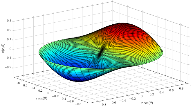
Figure 1: Solution $u(r,\theta)=r(1-r)\cos(\theta)$ of (24) with $g(\theta)=0$, $f(r,\theta)=-3\cos(\theta)$ and $R=1$.

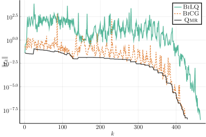
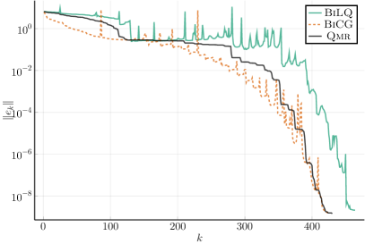
Figure 2: Convergence curves of BiLQ, BiCG and Qmr iterates on (24). The figures show the residual (left) and error (right) history for each method.

We also compare BiLQ with BiCG and Qmr on matrices SHERMAN5 and RAEFSKY1, with their respective right-hand side, from the UFL collection of Davis and Hu (2011). System SHERMAN5 has size $3,312$ with $20,793$ nonzeros and RAEFSKY1 has size $3,242$ with $293,409$ nonzeros. A Jacobi preconditioner is used for both systems.

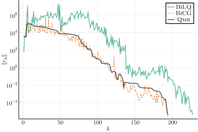
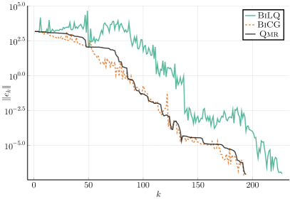
Figure 3: Convergence curves of BiLQ, BiCG and Qmr iterates for the SHERMAN5 system. The figures show the residual (left) and error (right) history for each method.

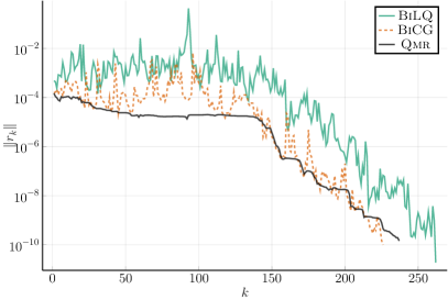
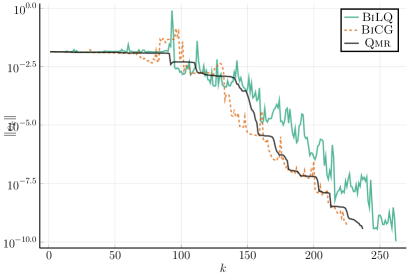
Figure 4: Convergence curves of BiLQ, BiCG and Qmr iterates for the RAEFSKY1 system. The figures show the residual (left) and error (right) history for each method.

Fig. 2, Fig. 3 and Fig. 4 all show that in BiLQ, neither the residual nor the error are monotonic in general. They also appear more erratic than those of Qmr. As in the symmetric case, both generally lag compared to those of BiCG and Qmr, but are not far behind. We experimented with other systems and observed the same qualitative behavior. As showed in section 2.6, although BiLQ is a minimum-error-type method, this error is minimized over a different space than that where $x^{\textup{\tiny L}}_{k}$ and $x^{\textup{\tiny C}}_{k}$ reside—see section 2.6. This situation is analogous to that between Symmlq and Cg in the symmetric case (Estrin et al., 2019c). Thus, the possibility of transferring to the BiCG point, when it exists, is attractive. Because the BiCG residual is easily computable, transferring based on the residual norm is readily implemented. The determination of upper bounds on the error suitable as stopping criteria remains the subject of active research (Estrin et al., 2019a, b, c).

2.8 Discussion

Like Qmr, the BiLQ iterate is well defined at each step even if $T_{k}$ is singular, whereas $x_{k}^{\textup{\tiny C}}$ is undefined when $\bar{\delta}_{k}=0$. A simple example is

$$A=\begin{bmatrix}0&-1\\ 1&\phantom{-}1\end{bmatrix},\qquad b=c=\begin{bmatrix}1\\ 0\end{bmatrix}.$$

According to Algorithm 1, $\beta_{1}=\gamma_{1}=1$, $v_{1}=u_{1}=b=c$. Then $\alpha_{1}=u_{1}^{T}Av_{1}=0$, $T_{1}=\begin{bmatrix}\alpha_{1}\end{bmatrix}$ is singular, and $T_{1}y_{1}=\beta_{1}$ is inconsistent. BiCG and its variants Cgs (Sonneveld, 1989) and BiCGStab (van der Vorst, 1992) all fail. However, $T_{2}$ is not singular and the BiCG point exists, although we cannot compute it without lookahead. In finite precision arithmetic, such exact breakdown are rather rare. But near-breakdowns ($\bar{\delta}_{k}\approx 0$) may happen and lead to numerical instabilities in ensuing iterations. An additional drawback of BiCG is that the LU decomposition of $T_{k}$ might not exist without pivoting even if $T_{k}$ is nonsingular whereas the LQ factorization of $T_{k-1,k}$ is always well defined.

3 Adjoint systems

Motivated by fuild dynamics applications, Pierce and Giles (2000) describe a method for doubling the order of accuracy of estimates of integral functionals involving the solution of a PDE. Consider a well-posed linear PDE $Lu=f$ on a domain $\Omega$ subject to homogeneous boundary conditions, where $L$ is a differential operator of the form (23) and $f\in L_{2}(\Omega)$. Suppose we wish to evaluate the functional $J(u):=\langle u,\,g\rangle$, where $g\in L_{2}(\Omega)$ and $\langle\cdot,\,\cdot\rangle$ represents an integral inner product on $L_{2}(\Omega)$. The problem may be stated equivalently as evaluating the functional $\langle v,\,f\rangle$ where $v$ solves the adjoint PDE $L^{*}v=g$ because $\langle v,\,f\rangle=\langle v,\,Lu\rangle=\langle L^{*}v,\,u\rangle=\langle g,\,u\rangle$.

Let the discretization of $L$ yield the linear system $Au_{D}=f_{D}$ with $D$ a set of points that define a grid on $\Omega$. For certain types of PDEs and certain discretization schemes, $A^{T}$ is an appropriate discretization of $L^{*}$. Pierce and Giles (2000) provide examples with linear operators such as Poisson’s equation discretized by finite differences in 1D and by finite elements in 2D, but their discretizations are symmetric. Their method also applies to cases where $A\neq A^{T}$ but in such cases, the discretization of the primal and dual equations commonly differ. Therefore, there is a need for methods that solve an unsymmetric primal system and its adjoint simultaneously. Lu and Darmofal (2003) and Golub et al. (2008) were also interested in this problem for scattering amplitude evaluation. Lu and Darmofal (2003) devise a modification of Qmr in which the two initial vectors are $b$ and $c$ and a quasi residual is minimized for both the primal and adjoint systems via an updated QR factorization. Golub et al. (2008) apply Usymqr (Saunders et al., 1988) to both the primal and the adjoint system simultaneously by updating two QR factorizations. The advantage of their approach is that it produces monotonic residuals for both systems.

Assume we use a method to compute $u_{D}$ and to solve $A^{T}v_{D}=g_{D}$ such that $\|u-u_{D}\|\in O(h^{p})$ and $\|v-v_{D}\|\in O(h^{p})$, where $h$ describes the grid coarseness. From $u_{D}$ and $v_{D}$ we compute approximations $u_{h}\approx u$ and $v_{h}\approx v$ over $\Omega$ by way of an interpolation of higher order than the discretization. Define $f_{h}:=Lu_{h}$ and $g_{h}:=L^{*}v_{h}$. Instead of $J(u)\approx\langle u_{h},\,g\rangle$, an approximation of order $p$, we may obtain one of order $2p$ via the identity

(25) $$\langle g,\,u\rangle=\langle g,\,u_{h}\rangle-\langle v_{h},\,f_{h}-f\rangle+\langle g_{h}-g,\,u_{h}-u\rangle.$$

The first two terms constitute our new approximation while the remaining error term can be expressed as $\langle g_{h}-g,L^{-1}(f_{h}-f)\rangle=O(h^{2p})$.

From this point, we consider, in addition to (1), the adjoint system

(26) $$A^{T}t=c.$$

Solving simultaneously primal and dual systems can also be formulated as solving the symmetric and indefinite system

(27) $$\begin{bmatrix}0&A\\ A^{T}&0\end{bmatrix}\begin{bmatrix}t\\ x\end{bmatrix}=\begin{bmatrix}b\\ c\end{bmatrix}.$$

Minres or Minres-qlp (Choi et al., 2011) are prime candidates for (27) and will serve as a basis for comparison.

In the context of Algorithm 1, we can take advantage of the two initial vectors $b$ and $c$ to combine BiLQ and Qmr and solve both the primal and adjoint systems simultaneously at no other extra cost than that of updating solution and residual estimates. We call the resulting method BiLQR. Contrary to the approach of Lu and Darmofal (2003), no extra factorization updates are necessary. Instead of approximating $u_{D}$ and $v_{D}$ by minimizing two quasi residuals, BiLQR minimizes one quasi residual and computes the second approximation via a minimum-norm subproblem.

A similar method based on the orthogonal tridiagonalization process of Saunders et al. (1988) can be derived by combining Usymlq and Usymqr, which we call TriLQR, and which is to the approach of Golub et al. (2008) as BiLQR is to that of Lu and Darmofal (2003). TriLQR remains well defined for rectangular $A$.

3.1 Description of BiLQR

BiLQR updates an approximate solution $t^{\textup{\tiny Q}}_{k-1}=U_{k-1}f^{\textup{\tiny Q}}_{k-1}$ of $A^{T}t=c$ by solving the Qmr least-squares subproblem

(28) $$\mathop{\textup{minimize}}_{f}\ \|T_{k-1,k}^{T}f-\gamma_{1}e_{1}\|\quad\Longleftrightarrow\quad\mathop{\textup{minimize}}_{f}\ \left\|\begin{bmatrix}L_{k-1}^{T}\\ 0\end{bmatrix}f-Q_{k}\gamma_{1}e_{1}\right\|$$

because the QR factorization of $T_{k-1,k}^{T}$ is readily available. Define $\bar{h}_{k}=Q_{k}\gamma_{1}e_{1}=(h_{k-1},\,\bar{\psi}_{k})=(\psi_{1},\,\cdots,\,\psi_{k-1},\,\bar{\psi}_{k})$. The components of $\bar{h}_{k}$ are updated according to

(29a) $$\bar{\psi}_{1} =\gamma_{1},$$

(29b) $$\psi_{k} =c_{k+1}\bar{\psi}_{k},~{}k\geq 1,$$

(29c) $$\bar{\psi}_{k+1} =s_{k+1}\bar{\psi}_{k},\quad k\geq 1.$$

The solution of (28) is $f^{\textup{\tiny Q}}_{k-1}=L_{k-1}^{-T}h_{k-1}$ and the least-squares residual norm is $|\bar{\psi}_{k}|$. To avoid storing $U_{k}$, we define $W_{k}=U_{k}L_{k}^{-T}$, which can be updated as

(30a) $$w_{1} =u_{1}/\delta_{1},$$

(30b) $$w_{2} =(u_{2}-\lambda_{1}w_{1})/\delta_{2},$$

(30c) $$w_{k} =(u_{k}-\lambda_{k-1}w_{k-1}-\varepsilon_{k-2}w_{k-2})/\delta_{k},\quad k\geq 3.$$

At the next iteration, $t^{\textup{\tiny Q}}_{k}$ can be recursively updated according to

$$t^{\textup{\tiny Q}}_{k}=U_{k}f^{\textup{\tiny Q}}_{k}=U_{k}L_{k}^{-T}h_{k}=W_{k}h_{k}=W_{k-1}h_{k-1}+\psi_{k}w_{k}=t^{\textup{\tiny Q}}_{k-1}+\psi_{k}w_{k}.$$

The Qmr residual is

$$r_{k}^{\textup{\tiny Q}}=c-A^{T}t^{\textup{\tiny Q}}_{k}=U_{k+1}(\gamma_{1}e_{1}-T_{k,k+1}^{T}f^{\textup{\tiny Q}}_{k})=\bar{\psi}_{k+1}U_{k+1}Q_{k+1}^{T}e_{k+1}^{T},$$

so that

$$\|r_{k}^{\textup{\tiny Q}}\|\leq\|U_{k+1}\|_{F}\,\|\bar{\psi}_{k+1}Q_{k+1}^{T}e_{k+1}^{T}\|\leq\|\bar{\psi}_{k+1}\|\sqrt{\tau_{k+1}},$$

where $\tau_{k+1}=\sum_{i=1}^{k+1}\|u_{i}\|^{2}=\tau_{k}+\|u_{k+1}\|^{2}$. If the $u_{k}$ are normalized, then $\tau_{k}=k$. Algorithm 4 states the complete procedure.

The following result states a minimization property of the Qmr residual in an iteration-dependent norm.

The $(k-1)$th Qmr iterate $t^{\textup{\tiny Q}}_{k-1}$ solves

(31) $$\mathop{\textup{minimize}}_{t}\,\|c-A^{T}t\|_{V_{k}V_{k}^{T}}\ \mathop{\textup{subject to}}\,t\in\mathop{\mathrm{Range}}(U_{k-1}).$$

In addition, $\|r^{\textup{\tiny Q}}_{k}\|_{V_{k}V_{k}^{T}}$ is monotonically decreasing.

Proof.

The set of constraints of (31) imposes that there exist $f\in\mathds{R}^{k-1}$ such that $t=U_{k-1}f$. By biorthogonality, the objective value at such an $t$ can be written $\|c-A^{T}U_{k-1}f\|_{V_{k}V_{k}^{T}}=\|c-U_{k}T_{k-1,k}^{T}f\|_{V_{k}V_{k}^{T}}=\|\gamma_{1}e_{1}-T_{k-1,k}^{T}f\|$. We recover the subproblem (28).

For the second part, $\|r^{\textup{\tiny Q}}_{k}\|_{V_{k+1}V_{k+1}^{T}}=|\bar{\psi}_{k+1}|=|s_{k+1}||\bar{\psi}_{k}|=|s_{k+1}|\|r^{\textup{\tiny Q}}_{k-1}\|_{V_{k}V_{k}^{T}}$.

Note that section 3.1 continues to hold if $r^{\textup{\tiny Q}}_{k}$ is measured in the $V_{p}V_{p}^{T}$-norm.

3.2 Description of TriLQR

The Saunders et al. (1988) tridiagonalization process generates sequences of vectors $\{v_{k}\}$ and $\{u_{k}\}$ such that $v_{i}^{T}v_{j}=\delta_{ij}$ and $u_{i}^{T}u_{j}=\delta_{ij}$ in exact arithmetic for as long as the process does not break down. The process is summarized as Algorithm 3.

Algorithm 3 Tridiagonalization Process

1:$A$, $b$, $c$

2:$v_{0}=0$, $u_{0}=0$

3:$\beta_{1}v_{1}=b$, $\gamma_{1}u_{1}=c$ $(\beta_{1},~{}\gamma_{1})>0$ so that $\|v_{1}\|=\|u_{1}\|=1$

4:for $k$ = 1, 2, $\dots$ do

5:     $q=Au_{k}-\gamma_{k}v_{k-1}$, $\alpha_{k}=v_{k}^{T}q$

6:     $p=A^{T}v_{k}-\beta_{k}u_{k-1}$

7:     $\beta_{k+1}v_{k+1}=q-\alpha_{k}v_{k}$ $\beta_{k+1}>0$ so that $\|v_{k+1}\|=1$

8:     $\gamma_{k+1}u_{k+1}=p-\alpha_{k}u_{k}$ $\gamma_{k+1}>0$ so that $\|u_{k+1}\|=1$

9:end for

At the end of the $k$-th iteration, we have

(32a) $$AU_{k} =V_{k}T_{k}~{}+\beta_{k+1}v_{k+1}e_{k}^{T}=V_{k+1}T_{k+1,k}$$

(32b) $$A^{T}V_{k} =U_{k}T_{k}^{T}+\gamma_{k+1}u_{k+1}e_{k}^{T}=U_{k+1}T_{k,k+1}^{T},$$

to be compared with (3).

Saunders et al. (1988) develop two methods based on Algorithm 3. Usymlq generates an approximation to a solution of (1) of the form $x^{\textup{\tiny LQ}}_{k}=U_{k}y^{\textup{\tiny LQ}}_{k}$, where $y^{\textup{\tiny LQ}}_{k}\in\mathds{R}^{k}$ solves

(33) $$\mathop{\textup{minimize}}_{y}\ \|y\|\quad\mathop{\textup{subject to}}\ T_{k-1,k}y=\beta_{1}e_{1}.$$

With (32) and (33), we have the following analogue of section 2.6 and (22).

Let $x_{\star}$ be the exact solution of (1). The $k$th Usymlq iterate $x^{\textup{\tiny LQ}}_{k}$ solves

(34) $$\mathop{\textup{minimize}}_{x}\,\|x\|\ \mathop{\textup{subject to}}\,x\in\mathop{\mathrm{Range}}(U_{k}),\ b-Ax\perp\mathop{\mathrm{Range}}(U_{k-1}),$$

and

(35) $$\mathop{\textup{minimize}}_{x}\,\|x-x_{\star}\|\ \mathop{\textup{subject to}}\,x\in\mathop{\mathrm{Range}}(A^{T}V_{k-1}).$$

Proof.

The proof is nearly identical to that of section 2.6 and relies on the fact that $r^{\textup{\tiny LQ}}_{k}:=b-Ax^{\textup{\tiny LQ}}_{k}$ is a combination of $u_{k}$ and $u_{k+1}$ (Buttari et al., 2019, §3.2.2).

The second method, Usymqr, generates an approximation $t^{\textup{\tiny QR}}_{k}=V_{k}f^{\textup{\tiny QR}}_{k}$ where $f^{\textup{\tiny QR}}_{k}\in\mathds{R}^{k}$ solves

(36) $$\mathop{\textup{minimize}}_{f}\ \|T_{k,k+1}^{T}f-\gamma_{1}e_{1}\|.$$

The following property applies to $t^{\textup{\tiny QR}}_{k}$ due to our assumption that (1) is consistent.

[Buttari et al., 2019, Theorem $1$] Assume $b\in\mathop{\mathrm{Range}}(A)$. Then Usymqr finds the minimum-norm solution of

$$\mathop{\textup{minimize}}_{t}\ \|A^{T}t-c\|.$$

Of course, $A$ nonsingular implies that the solution to (26) is unique but Algorithm 3 applies more generally to rectangular and/or rank-deficient $A$.

When $A=A^{T}$ and $b=c$, Algorithm 3 coincides with the symmetric Lanczos process, and Usymlq and Usymqr are equivalent to Symmlq and Minres (Paige and Saunders, 1975), respectively. Besides the orthogonalization process, differences between those methods and BiLQ and Qmr are the definition of $\bar{D}_{k}$ and $W_{k}$, and the fact that $u_{k}$ and $v_{k}$ are swapped. If stopping criteria are based on residual norms, expressions derived for methods based on Algorithm 1 apply to methods based on Algorithm 3, but their expressions can simplified because $V_{k}$ and $U_{k}$ are orthogonal. Usymqr and Usymlq can be combined into TriLQR to solve both the primal and ajoint system simultaneously. We summarize the complete procedure as Algorithm 5 and highlight lines with differences between the two algorithms.

Algorithm 4 BiLQR

1:$A$, $b$, $c$

2:$\beta_{1}v_{1}=b$, $\gamma_{1}u_{1}=c$

3:$\alpha_{1}=u_{1}^{T}Av_{1}$

4: $\beta_{2}v_{2}=Av_{1}-\alpha_{1}v_{1}$

5: $\gamma_{2}u_{2}=A^{T}u_{1}-\alpha_{1}u_{1}$

6:$c_{1}=-1$, $s_{1}=0$, $\bar{\delta}_{1}=\alpha_{1}$

7:$\eta_{1}=\beta_{1}$, $\bar{d}_{1}=v_{1}$, $\bar{\psi}_{1}=\gamma_{1}$

8:$x^{\textup{\tiny L}}_{1}=0$, $t^{\textup{\tiny Q}}_{0}=0$

9:for $k$ = 2, 3, $\dots$ do

10:      $q=Av_{k}-\gamma_{k}v_{k-1}$, $\alpha_{k}=u_{k}^{T}q$

11:      $p=A^{T}u_{k}-\beta_{k}u_{k-1}$

12:     $\beta_{k+1}v_{k+1}=q-\alpha_{k}v_{k}$

13:     $\gamma_{k+1}u_{k+1}=p-\alpha_{k}u_{k}$

14:     $\delta_{k-1}=(\bar{\delta}_{k-1}^{2}+\gamma_{k}^{2})^{\frac{1}{2}}$

15:     $c_{k}=\bar{\delta}_{k-1}/\delta_{k-1}$

16:     $s_{k}=\gamma_{k}/\delta_{k-1}$

17:     $\varepsilon_{k-2}=s_{k-1}\beta_{k}$

18:     $\lambda_{k-1}=-c_{k-1}c_{k}\beta_{k}+s_{k}\alpha_{k}$

19:     $\bar{\delta}_{k}=-c_{k-1}s_{k}\beta_{k}-c_{k}\alpha_{k}$

20:     $\zeta_{k-1}=\eta_{k-1}/\delta_{k-1}$

21:     $\eta_{k}=-\varepsilon_{k-2}\zeta_{k-2}-\lambda_{k-1}\zeta_{k-1}$

22:      $d_{k-1}=c_{k}\bar{d}_{k-1}+s_{k}v_{k}$

23:      $\bar{d}_{k}=s_{k}\bar{d}_{k-1}-c_{k}v_{k}$

24:     $\psi_{k-1}=c_{k}\bar{\psi}_{k-1}$

25:     $\bar{\psi}_{k}=s_{k}\bar{\psi}_{k-1}$

26:      $w_{k-1}=\frac{u_{k-1}-\lambda_{k-2}w_{k-2}-\varepsilon_{k-3}w_{k-3}}{\delta_{k-1}}$

27:     $x^{\textup{\tiny L}}_{k}=x^{\textup{\tiny L}}_{k-1}+\zeta_{k-1}d_{k-1}$

28:     $t^{\textup{\tiny Q}}_{k-1}=t^{\textup{\tiny Q}}_{k-2}+\psi_{k-1}w_{k-1}$

29:end for

30:if $\bar{\delta}_{k}\neq 0$ then

31:     $\bar{\zeta}_{k}=\eta_{k}/\bar{\delta}_{k}$

32:     $x^{\textup{\tiny C}}_{k}=x^{\textup{\tiny L}}_{k}+\bar{\zeta}_{k}\bar{d_{k}}$

33:end if

Algorithm 5 TriLQR

$A$, $b$, $c$

$\beta_{1}v_{1}=b$, $\gamma_{1}u_{1}=c$

$\alpha_{1}=u_{1}^{T}Av_{1}$

$\beta_{2}v_{2}=Au_{1}-\alpha_{1}v_{1}$

$\gamma_{2}u_{2}=A^{T}v_{1}-\alpha_{1}u_{1}$

$c_{1}=-1$, $s_{1}=0$, $\bar{\delta}_{1}=\alpha_{1}$

$\bar{\eta}_{1}=\beta_{1}$, $\bar{d}_{1}=u_{1}$, $\bar{\psi}_{1}=\gamma_{1}$

$x^{\textup{\tiny LQ}}_{1}=0$, $t^{\textup{\tiny QR}}_{0}=0$

for $k$ = 2, 3, $\dots$ do

      $q=Au_{k}-\gamma_{k}v_{k-1}$, $\alpha_{k}=v_{k}^{T}q$

      $p=A^{T}v_{k}-\beta_{k}u_{k-1}$

     $\beta_{k+1}v_{k+1}=q-\alpha_{k}v_{k}$

     $\gamma_{k+1}u_{k+1}=p-\alpha_{k}u_{k}$

     $\delta_{k-1}=(\bar{\delta}_{k-1}^{2}+\gamma_{k}^{2})^{\frac{1}{2}}$

     $c_{k}=\bar{\delta}_{k-1}/\delta_{k-1}$

     $s_{k}=\gamma_{k}/\delta_{k-1}$

     $\varepsilon_{k-2}=s_{k-1}\beta_{k}$

     $\lambda_{k-1}=-c_{k-1}c_{k}\beta_{k}+s_{k}\alpha_{k}$

     $\bar{\delta}_{k}=-c_{k-1}s_{k}\beta_{k}-c_{k}\alpha_{k}$

     $\zeta_{k-1}=\eta_{k-1}/\delta_{k-1}$

     $\eta_{k}=-\varepsilon_{k-2}\zeta_{k-2}-\lambda_{k-1}\zeta_{k-1}$

      $d_{k-1}=c_{k}\bar{d}_{k-1}+s_{k}u_{k}$

      $\bar{d}_{k}=s_{k}\bar{d}_{k-1}-c_{k}u_{k}$

     $\psi_{k-1}=c_{k}\bar{\psi}_{k-1}$

     $\bar{\psi}_{k}=s_{k}\bar{\psi}_{k-1}$

      $w_{k-1}=\frac{v_{k-1}-\lambda_{k-2}w_{k-2}-\varepsilon_{k-3}w_{k-3}}{\delta_{k-1}}$

     $x^{\textup{\tiny LQ}}_{k}=x^{\textup{\tiny LQ}}_{k-1}+\zeta_{k-1}d_{k-1}$

     $t^{\textup{\tiny QR}}_{k-1}=t^{\textup{\tiny QR}}_{k-2}+\psi_{k-1}w_{k-1}$

end for

if $\bar{\delta}_{k}\neq 0$ then

     $\bar{\zeta}_{k}=\eta_{k}/\bar{\delta}_{k}$

     $x^{\textup{\tiny CG}}_{k}=x^{\textup{\tiny LQ}}_{k}+\bar{\zeta}_{k}\bar{d_{k}}$

end if

BiLQR and TriLQR both need nine $n$-vectors: $u_{k}$, $u_{k-1}$, $v_{k}$, $v_{k-1}$, $w_{k}$, $w_{k-1}$, $\bar{d}_{k}$, $x_{k}$ and $t_{k-1}$ whereas Minres-qlp applied to (27) can be implemented with five $(2n)$-vectors. Two more $n$-vectors are needed when in-place “gemv” updates are not explicitly available. Table 2 summarizes the cost of BiLQR, TriLQR, Minres-qlp and variants from Lu and Darmofal (2003) and Golub et al. (2008), developed for adjoint systems. An advantage of Minres-qlp and TriLQR is that adjoint systems can be solved even if $b^{T}c=0$, which is not possible with BiLQR. In addition, serious breakdowns $q^{T}p=0$ with $p\neq 0$ and $q\neq 0$ are not a problem with TriLQR. TriLQR is similar in spirit to the recent method Usymlqr of Buttari et al. (2019) for solving symmetric saddle-point systems, but is slightly cheaper.

Table 2: Storage and cost per iteration of methods for solving (1) and (26) simultaneously.

	$n$-vectors	dots	scal	axpy
BiLQR	9	2	5	10
TriLQR	9	2	5	10
Minres-qlp	10	4	8	14
Lu and Darmofal (2003)	10	2	6	10
Golub et al. (2008)	10	2	6	10

3.3 Applications

For the purpose of a simple illustration, we consider a one-dimensional ODE and a two-dimensional PDE. Consider first the linear ODE with constant coefficients

(37a) $$\chi_{1}u^{\prime\prime}(x)+\chi_{2}u^{\prime}(x)+\chi_{3}u(x) =f(x)\quad x \in\Omega$$

(37b) $$u(x) =0\quad x \in\partial\Omega,$$

where $\Omega=[0,\,1]$, and say we are interested in the value of the linear functional

(38) $$J(u)=\int_{\Omega}u(x)g(x)\,\mathrm{d}\Omega,$$

where $u$ solves (37) and $g\in L_{2}(\Omega)$. The adjoint equation can be derived from (37) using integration by parts:

(39a) $$\chi_{1}v^{\prime\prime}(x)-\chi_{2}v^{\prime}(x)+\chi_{3}v(x) =g(x)\quad x \in\Omega$$

(39b) $$v(x) =0\quad x \in\partial\Omega.$$

Note that the only difference between the primal and adjoint equations resides in the sign of odd-degree derivatives. The discussion in Section 3 ensures that

(40) $$G(v):=\int_{\Omega}f(x)v(x)\,\mathrm{d}\Omega=J(u).$$

Consider the uniform discretization $x_{i}=ih$, $i=0,\dots,N+1$, where $h=1/(N+1)$. We use centered finite differences of order 2, i.e.,

$$u^{\prime}(x_{i})=\frac{u_{i+1}-u_{i-1}}{2h}+O(h^{2}),\quad u^{\prime\prime}(x_{i})=\frac{u_{i-1}-2u_{i}+u_{i+1}}{h^{2}}+O(h^{2}).$$

We obtain $u(x_{i})$ for $x_{i}\in D:=\{x_{i}\mid i\in 1,\dots,N\}$ from the tridiagonal linear system

$$\begin{bmatrix}-2\chi_{1}+\chi_{3}h^{2}&\chi_{1}+\chi_{2}h&&\\ \chi_{1}-\chi_{2}h&-2\chi_{1}+\chi_{3}h^{2}&\ddots&\\ &\ddots&\ddots&\chi_{1}+\chi_{2}h\\ &&\chi_{1}-\chi_{2}h&-2\chi_{1}+\chi_{3}h^{2}\end{bmatrix}\begin{bmatrix}u(x_{1})\\ \vdots\\ \vdots\\ u(x_{N})\end{bmatrix}=h^{2}\begin{bmatrix}f(x_{1})\\ \vdots\\ \vdots\\ f(x_{N})\end{bmatrix}.$$

More compactly, we write $Au_{D}=f_{D}$. Similarly, we compute $v(x_{i})$ for $x_{i}\in D$ from $A^{T}v_{D}=g_{D}$. Next, we compute an approximation of $u$ and $v$ over $\Omega$ by cubic spline interpolation, and the resulting functions are denoted $u_{h}$ and $v_{h}$. We impose that $Lu_{h}=f$ and $L^{*}v_{h}=g$ on $\partial\Omega$. We subsequently obtain $f_{h}(x):=\chi_{1}u_{h}^{\prime\prime}(x)+\chi_{2}u_{h}^{\prime}(x)+\chi_{3}u_{h}(x)$. The end points conditions of the cubic splines impose that $f_{h}$ coincide with $f$ on $\partial\Omega$. Finally, we compute the improved estimate (25) using a three-point Gauss quadrature to approximate each

$$\int_{x_{i}}^{x_{i+1}}g(x)u_{h}(x)\,\mathrm{d}x-\int_{x_{i}}^{x_{i+1}}v_{h}(x)(f_{h}(x)-f(x))\,\mathrm{d}x$$

on each subinterval to ensure that the numerical quadrature errors are smaller than the discretization error.

We choose $n=50$, $\chi_{1}=\chi_{2}=\chi_{3}=1$, $g(x)=e^{x}$ and $f(x)$ such that the exact solution of (37) is $u_{\star}(x)=sin(\pi x)$. The resulting linear system has dimension $50$ with $148$ nonzeros. Those parameters ensure that $J_{\star}=\langle g,\,u_{\star}\rangle=(\pi(e+1))/(\pi^{2}+1)$. Figs. 5 and 6 report the evolution of the residual and error on (1) and (26) for (37) and (39), respectively. BiLQR terminates in 51 iterations, TriLQR in 87 iterations and Minres-qlp in 198 iterations. The left plot of Fig. 7 illustrates the error in the evaluation of $J(u)$ as a function of $h$ using the naive $J(u)\approx J(u_{h})$ and improved (25) approximations.

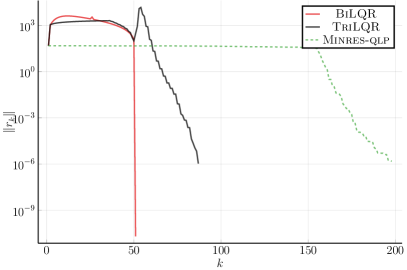
Figure 5: Residuals and errors norms of BiLQR, TriLQR and Minres-qlp iterates for on (37).

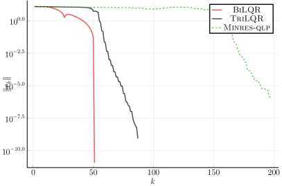
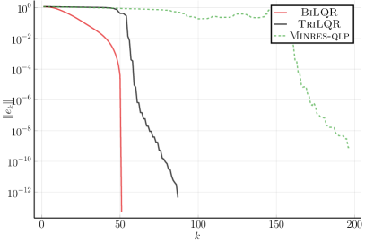
Figure 6: Residuals and errors norms of BiLQR, TriLQR and Minres-qlp iterates on (39).

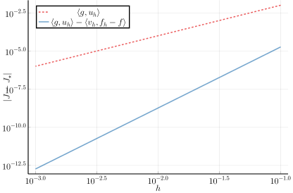
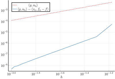
Figure 7: Functional evaluation errors for (37)–(39) (left) and (41)–(42) (right).

The steady-state convection-diffusion equation with constant coefficients

(41a) $$\kappa_{1}\Delta u(x)+\kappa_{2}\nabla\cdot u(x) =f(x)\quad x \in\Omega$$

(41b) $$u(x) =0\quad x \in\partial\Omega,$$

where $f\in L_{2}(\Omega)$, describes the flow of heat, particles, or other physical quantities in situations where there is both diffusion and convection or advection. Assume as before that we are interested in the linear functional (38). The adjoint equation of (41), again obtained via integration by parts, reads

(42a) $$\kappa_{1}\Delta v(x)-\kappa_{2}\nabla\cdot v(x) =g(x)\quad x \in\Omega$$

(42b) $$v(x) =0\quad x \in\partial\Omega,$$

and duality ensures (40).

In the case of heat transfer, $u(x)$ represents temperature and $f(x)$ sources or sinks. For example, with $g(x)=1/\mathop{\text{vol}}(\Omega)$, $J(u)$ represents the average temperature in $\Omega$.

We choose $\Omega=[0,\,1]\times[0,\,1]$ and descretize (41) on a uniform $N\times N$ grid with the finite difference method such that the step along both coordinates is $h=1/(N+1)$. With centered second-order differences for first and second derivatives, the discretized operator has the structure

$$A=\begin{bmatrix}T&D_{U}&&\\ D_{L}&T&\ddots&\\ &\ddots&\ddots&D_{U}\\ &&D_{L}&T\end{bmatrix},\hskip 433.62pt minus 433.62ptT=\begin{bmatrix}\text{\small$-4\kappa_{1}$}&\text{\small$\kappa_{1}+\tfrac{1}{2}\kappa_{2}h$}&&\\ \text{\small$\kappa_{1}-\tfrac{1}{2}\kappa_{2}h$}&\text{\small$-4\kappa_{1}$}&\ddots&\\ &\ddots&\ddots&\text{\small$\kappa_{1}+\tfrac{1}{2}\kappa_{2}h$}\\ &&\text{\small$\kappa_{1}-\tfrac{1}{2}\kappa_{2}h$}&\text{\small$-4\kappa_{1}$}\end{bmatrix},$$

$D_{U}=\mathop{\text{diag}}(\kappa_{1}+\tfrac{1}{2}\kappa_{2}h)$, $D_{L}=\mathop{\text{diag}}(\kappa_{1}-\tfrac{1}{2}\kappa_{2}h)$, where the right-hand sides $b$ and $c$ include the $h^{2}$ term. Solutions $u_{D}$ and $v_{D}$ contain an approximation of $u$ and $v$ at grid points stored column by column. The discretization of (42) with the same scheme yields $A^{T}$. We compare BiLQR, TriLQR and Minres-qlp on (41) and (42) with $\kappa_{1}=5$, $\kappa_{2}=20$, $N=50$, $g(x,y)=e^{x+y}$ and $f(x,y)$ such that the exact solution of (41) is $u_{\star}(x,y)=\sin(\pi x)\sin(\pi y)$. The resulting linear system has dimension $2,500$ with $12,300$ nonzeros. We use an absolute tolerance $\varepsilon_{a}=10^{-10}$ and a relative tolerance $\varepsilon_{r}=10^{-7}$, and terminate when both $\|r_{k}\|\leq\varepsilon_{a}+\|b\|\varepsilon_{r}$ for (1) and $\|r_{k}\|\leq\varepsilon_{a}+\|c\|\varepsilon_{r}$ for (26) hold.

Figs. 8 and 9 report the evolution of the residual and error on (1) and (26) for (41) and (42), respectively. In this numerical illustration, residuals and errors are computed explicitly at each iteration as $b-Ax$, $c-A^{T}t$, $x-x_{\star}$, and $t-t_{\star}$ in order to discount errors in the approximation formulae for those expressions. In this example, BiLQR terminates in about four times fewer iterations than TriLQR and six times fewer iterations than Minres-qlp. Only the Usymlq error and the Usymqr residual are monotonic. Although the Minres-qlp residual on (27) is monotonic, individual residuals on (1) and (26) are not.

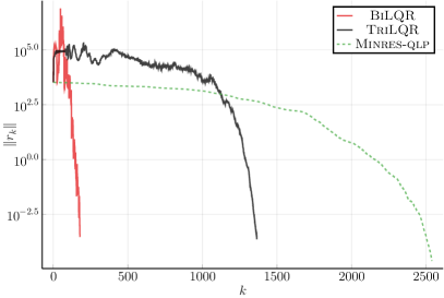
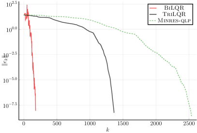
Figure 8: Residuals and errors norms of BiLQR, TriLQR and Minres-qlp iterates for on (41).

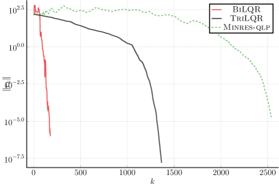
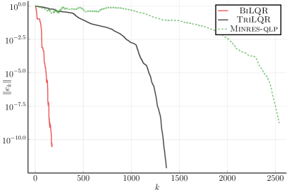
Figure 9: Residuals and errors norms of BiLQR, TriLQR and Minres-qlp iterates on (42).

We use bicubic spline interpolation and $3\times 3$ points Gauss quadrature to computate estimates of $J(u)$ with and without correction term. With the $u_{\star}$ given above, $J_{\star}:=J(u_{\star})=(\pi(e+1))^{2}/(\pi^{2}+1)^{2}$. The right plot of Fig. 7 illustrates the error in the evaluation of $J(u)$ as a function of $h$ using the naive $J(u)\approx J(u_{h})$ and improved (25) approximations.

4 Discussion

BiLQ completes the family of Krylov methods based on the Lanczos biorthogonalization process, and is a natural companion to BiCG and Qmr. It is a quasi-minimum error method, and in general, neither the error not the residual norm are monotonic.

Contrary to the Arnoldi (1951) and the Golub and Kahan (1965) processes, the Lanczos biorthogonalization and orthogonal trigonalization processes require two initial vectors. This distinguishing feature makes them readily suited to the simultaneous solution of primal and adjoint systems. A prime application is the superconvergent estimation of integral functionals in the context of discretized ODEs and PDEs. In our experiments, we observed that BiLQR outperforms both TriLQR and Minres-qlp applied to an augmented system in terms of error and residual norms.

Our Julia implementation of BiLQ, Qmr, BiLQR, TriLQR and Minres-qlp are available from github.com/JuliaSmoothOptimizers/Krylov.jl and can be applied in any floating-point arithmetic supported by the language. In our experiments with adjoint systems, we run both the primal and ajoint solvers until both residuals are small. A slightly more sophisticated implementation would interrupt the first solver that converges and only apply the other until it too converges. That is the strategy applied by Buttari et al. (2019).

Minres applied to (27) does not produce monotonic residuals in the individual primal and adjoint systems. In our experiments, we explicitly computed those residuals but Herzog and Soodhalter (2017) devised a modification of Minres that allows to monitor block residuals that could be of use in the context of estimating integral functionals.

Although the BiLQ error is not monotonic in the Euclidean norm, it is in the $U_{p}U_{p}^{T}$-norm, which is not iteration dependent, but is unknown until the end of the biorthogonalization process. The same property holds for the Qmr residual. Exploiting such properties to obtain useful bounds on the BiLQ and BiCG error in Euclidean norm that could help devise useful stopping criteria is the subject of ongoing research.

References

- Arnoldi [1951] W. E. Arnoldi. The principle of minimized iterations in the solution of the matrix eigenvalue problem. Q. Appl. Math., 9:17–29, 1951. 10.1090/qam/42792.
- Bezanson et al. [2017] J. Bezanson, A. Edelman, S. Karpinski, and V. B. Shah. Julia: A fresh approach to numerical computing. SIAM Rev., 59(1):65–98, 2017. 10.1137/141000671.
- Buttari et al. [2019] A. Buttari, D. Orban, D. Ruiz, and D. Titley-Peloquin. USYMLQR: A tridiagonalization method for symmetric saddle-point systems. SIAM J. Sci. Comput., 2019. To appear.
- Chisholm and Zingg [2009] T. T. Chisholm and D. W. Zingg. A Jacobian-free Newton-Krylov algorithm for compressible turbulent fluid flows. J. Comput. Phys., 228:3490–3507, 2009. 10.1016/j.jcp.2009.02.004.
- Choi et al. [2011] S. T. Choi, C. C. Paige, and M. A. Saunders. MINRES-QLP: A Krylov subspace method for indefinite or singular symmetric systems. SIAM J. Sci. Comput., 33(4):1810–1836, 2011.
- Davis and Hu [2011] T. Davis and Y. Hu. The University of Florida sparse matrix collection. ACM Trans. Math. Software, 38(1):1–25, 2011. 10.1145/2049662.2049663.
- Davis and Natarajan [2012] T. A. Davis and E. P. Natarajan. Sparse matrix methods for circuit simulation problems. In Scientific computing in electrical engineering SCEE 2010. Selected papers based on the presentations at the 8th conference, Toulouse, France, September 2010, pages 3–14. Springer, Berlin, 2012.
- Estrin et al. [2019a] R. Estrin, D. Orban, and M. A. Saunders. LSLQ: An iterative method for least-squares with an error minimization property. SIAM J. Matrix Anal. Appl., 40(1):254–275, 2019a. 10.1137/17M1113552.
- Estrin et al. [2019b] R. Estrin, D. Orban, and M. A. Saunders. LNLQ: An iterative method for least-norm problems with an error minimization property. SIAM J. Matrix Anal. Appl., 40(3):1102–1124, 2019b. 10.1137/18M1194948.
- Estrin et al. [2019c] R. Estrin, D. Orban, and M. A. Saunders. Euclidean-norm error bounds for SYMMLQ and CG. SIAM J. Matrix Anal. Appl., 40(1):235–253, 2019c. 10.1137/16M1094816.
- Fletcher [1976] R. Fletcher. Conjugate gradient methods for indefinite systems. In Numerical analysis, pages 73–89. Springer, 1976. 10.1007/BFb0080116.
- Freund and Nachtigal [1991] R. W. Freund and N. M. Nachtigal. QMR: a quasi-minimal residual method for non-Hermitian linear systems. Numer. Math., 60(1):315–339, 1991. 10.1007/BF01385726.
- Golub and Kahan [1965] G. H. Golub and W. Kahan. Calculating the singular values and pseudo-inverse of a matrix. SIAM J. Numer. Anal., 2(2):205–224, 1965. 10.1137/0702016.
- Golub et al. [2008] G. H. Golub, M. Stoll, and A. Wathen. Approximation of the scattering amplitude and linear systems. ETNA, 31(2008):178–203, 2008.
- Herzog and Soodhalter [2017] R. Herzog and K. Soodhalter. A modified implementation of MINRES to monitor residual subvector norms for block systems. SIAM J. Sci. Comput., 39(6):A2645–A2663, 2017. 10.1137/16M1093021.
- Hestenes and Stiefel [1952] M. R. Hestenes and E. Stiefel. Methods of conjugate gradients for solving linear systems. J. Res. Natl. Bur. Stand., 49(6):409–436, 1952. 10.6028/jres.049.044.
- Lai [2001] M. Lai. A note on finite difference discretizations for Poisson equation on a disk. Numer. Meth. Part. D. E., 17(3):199–203, 2001. 10.1002/num.1.
- Lanczos [1950] C. Lanczos. An iteration method for the solution of the eigenvalue problem of linear differential and integral operators. J. Res. Natl. Bur. Stand., 45:225–280, 1950. 10.6028/jres.045.026.
- Lu and Darmofal [2003] J. Lu and D. Darmofal. A quasi-minimal residual method for simultaneous primal-dual solutions and superconvergent functional estimates. SIAM J. Sci. Comput., 24(5):1693–1709, 2003. 10.1137/S1064827501390625.