The influence of the Earth’s curved spacetime on Gaussian quantum coherence

Abstract

Light wave-packets propagating from the Earth to satellites will be deformed by the curved background spacetime of the Earth, thus influencing the quantum state of light. We show that Gaussian coherence of photon pairs, which are initially prepared in a two-mode squeezed state, is affected by the curved spacetime background of the Earth. We demonstrate that quantum coherence of the state increases for a specific range of height $h$ and then gradually approaches a finite value with further increasing height of the satellite’s orbit in Kerr spacetime, because special relativistic effect are involved. Meanwhile, we find that Gaussian coherence increases with the increase of Gaussian bandwidth parameter, but the Gaussian coherence decreases with the growth of the peak frequency. In addition, we also find that total gravitational frequency shift causes changes of Gaussian coherence less than $\%1$ and different initial peak frequencies also can effect rate of change with the satellite height in geostationary Earth orbits.

I Introduction

The coherent superposition of states stands as one of the characteristic features that mark the departure of quantum mechanics from the classical realm E.P.C . Unlike quantum entanglement, discord, quantum coherence can exist in single systems, and can be achieved efficiently or impossible by classical methods. Quantum coherence constitutes a powerful resource for quantum metrology EPC1 ; EPC2 and entanglement creation EPC3 ; EPC4 and is the fundamental physical explanation of a series of intriguing phenomena in quantum optics EPC5 ; EPC6 ; EPC7 ; EPC8 and quantum information EPC9 . Viewing quantum coherence as resources is crucial for developing new quantum technologies. Recently, the necessary criteria for valid quantifiers of coherence and the rigorous characterizations of coherence in the framework of resource theories have been put forward in EPC10 ; EPC11 ; EPC12 ; EPC13 . Whereafter, a subsequent stream of works has identified coherence measures for both theoretical and experimental purposes HMW ; Skrzypczyk ; Kocsis ; Adesso2015 ; steering3 ; steering4 ; MWZZ ; steering5 ; Walborn ; steering2 ; Bowles ; VHTE . However, more attention has been given to quantum coherence without relativity effects, only little is known about behaviors of quantum coherence in a relativistic setting or curved spacetime background. Recently, quantum coherence had been studied in the dynamical Casimir effect in DSSC . In addition, it has been given to the dynamics of quantum coherence under the accelerated motions TBM .

Since realistic quantum systems always exhibit gravitational and relativistic features, quantum system cannot be prepared and transmitted in a curved spacetime without any gravitational and relativistic effects, the study of quantum coherence in a relativistic framework is necessary. Understand the influence of gravitational effects on the coherence quantum resource has practical and fundamental significance in realistic world when the parties involved are located at large distances in the curved space time DSSC ; TBM . The curved background spacetime of the Earth affects the running of quantum clocks, is employed as witnesses of general relativistic proper time in laser interferometric Zych , and influences the implementation of quantum metrology MADE ; MADE2 in satellite-based setups has been proposed in Refs Alclock ; wangsyn . Kish and Ralph found that there would be inevitable losses of quantum resources in the estimation of the Schwarzschild radius SPK . Furthermore Satellite-based quantum steering under the influence of spacetime curvature of the Earth had been proposed in Ref. TQJJH .

In this work, we present a quantitative investigation of Gaussian quantum coherence for correlated photon pairs which are initially prepared in a two-mode squeezed state under the curved background spacetime of the Earth. We assume that one of entangled photons stay at Earth’s surface and the other propagates to the satellite. During this propagation, the photons’ wave-packet will be deformed by the curved background spacetime of the Earth, and these deformations effects on the quantum state of the photons can be modeled as a lossy quantum channel MANI . We quantitative calculate how much the losses of Gaussian quantum coherence and also discuss the behaviors of Gaussian coherence under the gravity of the Earth.

This work is organized as follows. In section II, we introduce the quantum field theory of a massless uncharged bosonic field which propagates from the Earth to a satellite. In section III, we briefly introduce the definition of the measurement of a bipartite Gaussian quantum coherence. In section IV, we show a scheme to test large distance quantum coherence between the Earth and satellites and study the behaviors of quantum coherence in the curved spacetime. The last section is devoted to a brief summary. Throughout the whole paper we employ natural units $G=c=\hbar=1$.

II Light wave-packets propagating on Earth’s space-time

In this section we will a briefly introduce about the propagation of photons from the Earth to satellites under the influence of the Earth’s gravitational field DEBT . The Earth’s spacetime can be approximately described by the Kerr metric Visser . For the sake of simplicity, our work will be constrained to the equatorial plane $\theta=\frac{\pi}{2}$. The reduced metric in Boyer-Lindquist coordinates $(t,r,\phi)$ reads Visser

$$ds^{2}= \,-\Big{(}1-\frac{2M}{r}\Big{)}dt^{2}+\frac{1}{\Delta}dr^{2}$$

$$\,+\Big{(}r^{2}+a^{2}+\frac{2Ma^{2}}{r}\Big{)}d\phi^{2}-\frac{4Ma}{r}dt\,d\phi,$$ (1)

$$\Delta= \,1-\frac{2M}{r}+\frac{a^{2}}{r^{2}},$$ (2)

where $M$, $r$, $J$, $a=\frac{J}{M}$ are the mass, radius, angular momentum and Kerr parameter of the Earth, respectively.

In order to better describe the propagation of wave-packets from a source on Earth to a receiver satellite situated at a fixed distance from the source this process, we assume Alice on Earth’s surface (i.e. $r_{A}=r_{E}$) and Bob who is on a satellite at a radius $r_{B}$. A photon is sent from Alice to Bob at time $\tau_{A}$, Bob will receive this photon at $\tau_{B}=\Delta\tau+\sqrt{f(r_{B})/f(r_{A})}\tau_{A}$ in his own reference frame, where $f(r_{A})=1-\frac{r_{S}}{r_{A}}$ and $f(r_{B})=1-\frac{r_{S}}{r_{B}}$. Here $r_{S}=2M$ is the Schwarzschild radius of the Earth and $\Delta\tau$ is the propagation time of the light from the Earth to the satellite by taking curved effects of the Earth into account. Realistic photon sources do not produce monochromatic photons, a photon can be modeled by a wave packet of excitations of a massless bosonic field with a distribution $F^{(K)}_{\Omega_{K,0}}$ of mode frequency $\Omega_{K}$ and peaked at $\Omega_{K,0}$ ULMQ ; TGDT , where $K=A,B$ denote the modes in Alice’s or Bob’s reference frames, respectively. The annihilation operator for the photon for an observer infinitely far from Alice or Bob, takes the form

$$\hat{a}_{\Omega_{K,0}}(t_{K})=\int_{0}^{+\infty}d\Omega_{K}e^{-i\Omega_{K}t_{K}}F^{(K)}_{\Omega_{K,0}}(\Omega_{K})\hat{a}_{\Omega_{K}}.$$ (3)

Alice’s and Bob’s operators in Eq. (3) can be used to describe the same optical mode in different altitudes. The photon’s creation $\hat{a}^{\dagger}_{\Omega_{K,0}}$ and annihilation operators $\hat{a}_{\Omega_{K,0}}$ satisfy the canonical equal time bosonic commutation $[\hat{a}_{\Omega_{K,0}}(t),\hat{a}^{\dagger}_{\Omega_{K,0}}(t)]=1$ relations when the frequency distribution $F^{(K)}(\Omega)$ is normalized, that is $\int_{\Omega>0}|F^{(K)}(\Omega)|^{2}=1$. This distribution naturally models a photon which is a wave packet of the electromagnetic field that propagates and is localized in space and time.

Considering the Earth’s gravitational field between Alice and Bob, the wave packet received by Bob is modified when Alice sent a wave packet of the photon. The relation between $\hat{a}_{\Omega_{A}}$ and $\hat{a}_{\Omega_{B}}$ was discussed in DEBT ; DEBA ; wangsyn , and can be used to calculate the relation between the frequency distributions $F^{(K)}_{\Omega_{K,0}}$ of the photons before and after the propagation

$$F^{(B)}_{\Omega_{B,0}}(\Omega_{B})=\sqrt[4]{\frac{f(r_{B})}{f(r_{A})}}F^{(A)}_{\Omega_{A,0}}\left(\sqrt{\frac{f(r_{B})}{f(r_{A})}}\Omega_{B}\right).$$ (4)

From Eq. (4), we can see that the effect induced by the curved spacetime of the Earth cannot be simply corrected by a linear shift of frequencies. Therefore, it may be challenging to compensate the transformation induced by the curvature in realistic implementations.

Indeed, such a nonlinear gravitational effect is found to influence the fidelity of the quantum channel between Alice and Bob DEBT ; DEBA ; wangsyn . It is always possible to decompose the mode $\bar{a}^{\prime}$ received by Bob in terms of the mode $a^{\prime}$ prepared by Alice and an orthogonal mode $\hat{a}_{\bot}^{\prime}$ (i.e. $[\hat{a}^{\prime},\hat{a}_{\bot}^{\prime\dagger}]=0$) PPRW

$$\bar{a}^{\prime}=\Theta\hat{a}^{\prime}+\sqrt{1-\Theta^{2}}\hat{a}_{\bot}^{\prime},$$ (5)

where $\Theta$ is the wave packet overlap between the distributions $F^{(B)}_{\Omega_{B,0}}(\Omega_{B})$ and $F^{(A)}_{\Omega_{A,0}}(\Omega_{B})$ which is given by

$$\Theta:=\int_{0}^{+\infty}d\Omega_{B}\,F^{(B)\star}_{\Omega_{B,0}}(\Omega_{B})F^{(A)}_{\Omega_{A,0}}(\Omega_{B}).$$ (6)

For $\Theta=1$ corresponds to a perfect channel and the channel between him and Alice (i.e., the spacetime) is noisy with $\Theta<1$. The quality of the channel can be quantified by employing the fidelity $\mathcal{F}=|\Theta|^{2}$.  Since the source is not monochromatic, we need a frequency distribution for the mode. We assume that Alice employs a real normalized Gaussian wave packet

$$F_{\Omega_{0}}(\Omega)=\frac{1}{\sqrt[4]{2\pi\sigma^{2}}}e^{-\frac{(\Omega-\Omega_{0})^{2}}{4\sigma^{2}}},$$ (7)

with wave packet width $\sigma$. In this case the overlap $\Theta$ is given by (6) where we have extended the domain of integration to all the real axis. We note that the integral should be performed over strictly positive frequencies. This is justified since the peak frequency is typically much larger than the spreading of the wave packet (i.e.,$\Omega_{0}\gg\sigma$). Thus, it is possible to include negative frequencies without affecting the value of $\Theta$. Employing Eqs. (3) and (7) one finds that

$$\Theta=\sqrt{\frac{2}{1+(1+\delta)^{2}}}\frac{1}{1+\delta}e^{-\frac{\delta^{2}\Omega_{B,0}^{2}}{4(1+(1+\delta)^{2})\sigma^{2}}},$$ (8)

where the new parameter $\delta$ quantifying the shifting is defined by

$$\delta=\sqrt[4]{\frac{f(r_{A})}{f(r_{B})}}-1=\sqrt{\frac{\Omega_{B}}{\Omega_{A}}}-1.$$ (9)

The expression for $\frac{\Omega_{B}}{\Omega_{A}}$ in the equatorial plane of the Kerr spacetime has been shown in kerr

$$\frac{\Omega_{B}}{\Omega_{A}}=\frac{1+\epsilon\frac{a}{r_{B}}\sqrt{\frac{M}{r_{B}}}}{C\sqrt{1-3\frac{M}{r_{B}}+2\epsilon\frac{a}{r_{B}}\sqrt{\frac{M}{r_{B}}}}},$$ (10)

where $C=[1-\frac{2M}{r_{A}}(1+2a{\omega})+\big{(}r^{2}_{A}+a^{2}-\frac{2Ma^{2}}{r_{A}}\big{)}{\omega}^{2}]^{-\frac{1}{2}}$ is the normalization constant, $\omega$ is the Earth’s equatorial angular velocity and $\epsilon=\pm 1$ stand for the direct of orbits (i.e., when $\epsilon=+1$ for the satellite co-rotates with the Earth). In the Schwarzschild limit $a,\omega\rightarrow 0$, Eq. (10) coincides to the result found in DEBT , which is

$$\frac{\Omega_{B}}{\Omega_{A}}=\sqrt{\frac{1-\frac{2M}{r_{A}}}{1-\frac{3M}{r_{B}}}}.$$ (11)

In order to obtain the explicit expression of the frequency shift for the photon exchanged between Alice and Bob, we expand the Eq. (10) and obtain the following perturbative expression for $\delta$ by $(r_{A}\omega)^{2}>a\omega$, therefore we can retain second order terms in $r_{A}\omega$. This perturbative result does not depend on whether the Earth and the satellite are co-rotating or not

$$\delta = \delta_{Sch}+\delta_{rot}+\delta_{h}$$

$$= \frac{1}{8}\frac{r_{S}}{r_{A}}\big{(}\frac{1-2\frac{h}{r_{A}}}{1+\frac{h}{r_{A}}}\big{)}-\frac{(r_{A}\omega)^{2}}{4}-\frac{(r_{A}\omega)^{2}}{4}\big{(}\frac{3}{4}\frac{r_{S}}{r_{A}}-\frac{4Ma}{\omega r_{A}^{3}}\big{)},$$

where $h=r_{B}-r_{A}$ is the height between Alice and Bob, $\delta_{Sch}$ is the first order Schwarzschild term, $\delta_{rot}$ is the lowest order rotation term and $\delta_{h}$ denotes all higher order correction terms. If the parameter $\delta=0$ (i. e. the satellite moves at the height $h\simeq\frac{r_{A}}{2}$), we have $\Theta=1$. The height at which the gravitational effect of the Earth and the special relativistic effect (i.e., doppler effect) due to the motion of the satellite compensate each other. That is to say, the received photons by Bob at this height will not experience any frequency shift and Bob’s clock rate becomes equal to the clock rate of Alice in this height. Indeed, the satellite’s motion around the Earth slows down Bob’s proper time, but the higher altitude of Bob introduces a lower redshift which therefore has also a lower effect on Bob’s clock rate, as compared to Alice. Meanwhile, the relevant limit of the expression for $\frac{\Omega_{B}}{\Omega_{A}}$ that in Minkowski is equal to $1$.

III Quantifying coherence of Gaussian states

In this section we briefly review the measurement of quantum coherence for a general two-mode Gaussian state $\rho_{AB}$ which is composed of a subsystem A and a subsystem B weedbrook . Then we can define the vector of the field quadratures as $\hat{R}=(\hat{x}^{A},\hat{p}^{A},\hat{x}^{B},\hat{p}^{B})^{\sf T}$, which satisfies the canonical commutation relations $[{{{\hat{R}}_{k}},{{\hat{R}}_{l}}}]=i{\Omega_{kl}}$, with $\Omega={{\ 0\ \ 1}\choose{-1\ 0}}^{\bigoplus{2}}$ being the symplectic form. All Gaussian properties can be determined from the symplectic form of the covariance matrix (CM) defined as ${\sigma_{ij}}=\text{Tr}\big{[}{{{\{{{{\hat{R}}_{i}},{{\hat{R}}_{j}}}\}}_{+}}\ {\rho_{AB}}}\big{]}$ RSP ; RSP1 ; RSP2 ; RSP3

$$\sigma_{AB}=\left(\!\!\begin{array}[]{cccc}a&0&c_{1}&0\\ 0&a&0&-c_{2}\\ c_{1}&0&b&0\\ 0&-c_{2}&0&b\end{array}\!\!\right).$$ (16)

The correlations $a$, $b$, $c_{1}$ and $c_{2}$ are determined by the four local symplectic invariants $I_{1}=a^{2}$, $I_{2}=b^{2}$, $I_{3}=c_{1}c_{2}$ and $I_{4}=\det(\sigma_{AB})=(ab-c_{1}^{2})(ab-c_{2}^{2})$. The symplectic eigenvalues of the CM of a two-mode Gaussian state are given as $2{\nu}_{\mp}^{2}=\Delta\mp\sqrt{\Delta^{2}-4I_{4}}$ with $\Delta=I_{1}+I_{2}+2I_{3}$ RSP2 ; RSP3 .

The coherence measure $C(\rho_{AB})$ has been given in terms of the displacement vectors and covariance matrix in JWX . Then we use the coherence measure as $C(\rho_{AB})=\inf{S(\rho_{AB}||\delta_{AB})}$, where $\delta_{AB}$ is the nearest incoherent Gaussian state of $\rho_{AB}$. The von Neumann entropy of a bipartite system $\rho_{AB}$ in terms of the symplectic eigenvalues is given by RSP5

$$S(\rho_{AB})=f({\nu}_{-})+f({\nu}_{+}),$$ (17)

where $f(\nu)=\frac{\nu+1}{2}\log_{2}\frac{\nu+1}{2}-\frac{\nu-1}{2}\log_{2}\frac{\nu-1}{2}$, while the mean occupation value is JWX

$$\overline{n}_{k}=\frac{1}{4}(\sigma_{11}^{k}+\sigma_{22}^{k}+[d_{1}^{k}]^{2}+[d_{2}^{k}]^{2}).$$ (18)

Here, $\sigma^{1}$ and $\sigma^{2}$ are elements of the subsystem of A and B in CM, respectively, and $[d^{k}_{i}]^{2}$ is $i$ first statistical moment of the $k$ mode. For convenience, we select $d^{k}_{1}=d^{k}_{2}=0$. It is possible to obtain an analytical expression of the quantum coherence of Gaussian states JWX

$$C({\rho_{AB}})= - S(\rho_{AB})+\Sigma_{i=1}^{2}[(\overline{n}_{i}+1)\log_{2}(\overline{n}_{i}+1)$$ (19)

$$- \overline{n}_{i}\log_{2}\overline{n}_{i}].$$

IV The influence of gravitational effect on Gaussian coherence

In this section we propose a scheme to test large distance quantum coherence between two satellites with different heights and discuss how quantum coherence is affected by the curved spacetime of the Earth. Firstly, we consider a pair of entangled photons which are initially prepared in a two-mode squeezed state with modes $b_{1}$ and $b_{2}$ at the ground station. Then we send one photon with mode $b_{1}$ to Alice. The other photon in mode $b_{2}$ propagates from the Earth to the satellite and is received by Bob (at the height $h_{B}=r_{B}-r_{A}$). Due to the curved background spacetime of the Earth, the wave packet of photons are deformed. Finally, we study the behavior of Gaussian coherence under the Earth’s gravitational field.

Considering that Alice receives the mode $b_{1}$ and Bob receives the mode $b_{2}$ at different satellite orbits, we should take the curved spacetime of the Earth into account. As discussed in DEBT ; DEBA ; wangsyn , the influence of the Earth’s gravitational effect can be modeled by a beam splitter with orthogonal modes $b_{1\bot}$ and $b_{2\bot}$. The covariance matrix of the initial state is given by

$$\Sigma^{b_{1}b_{2}b_{1\bot}b_{2\bot}}_{0}=\left(\begin{array}[]{cc}\tilde{\sigma}(s)&0\\ 0&I_{4}\end{array}\right),$$ (20)

where ${I}_{4}$ denotes the $4\times 4$ identity matrix and $\tilde{\sigma}{(s)}$ is the covariance matrix of the two-mode squeezed state

$$\tilde{\sigma}(s)=\left(\begin{array}[]{cc}\cosh{(2s)}{I}_{2}&\sinh{(2s)}\sigma_{z}\\ \sinh(2s)\sigma_{z}&\cosh{(2s)}{I}_{2}\end{array}\right),$$ (21)

where $\sigma_{z}$ is Pauli matrix and $s$ is the squeezing parameter. The effects induced by the curved spacetime of the Earth on Alice’s mode $b_{1}$ and Bob’s mode $b_{2}$ can be model as lossy channel, which are described by the transformation DEBT ; DEBA ; wangsyn

$$\bar{b}_{1} = \Theta_{1}\,b_{1}+\sqrt{{1-\Theta_{1}^{2}}}b_{1\bot},$$ (22)

$$\bar{b}_{2} = \Theta_{2}\,b_{2}+\sqrt{{1-\Theta_{2}^{2}}}b_{2\bot}.$$ (23)

This process can be represented as a mixing (beam splitting ) of modes $b_{1}(b_{2})$ and $b_{1\bot}(b_{2\bot})$. Therefore, for the entire state, the symplectic transformation can be encoded into the Bogoloiubov transformation

$$S=\left(\begin{array}[]{cccc}\Theta_{1}{I}_{2}&0&\sqrt{1-\Theta_{1}^{2}}&0\\ 0&\Theta_{2}{I}_{2}&0&\sqrt{1-\Theta_{2}^{2}}{I}_{2}\\ \sqrt{1-\Theta_{1}^{2}}&0&-\Theta_{1}{I}_{2}&0\\ 0&\sqrt{1-\Theta_{2}^{2}}{I}_{2}&0&-\Theta_{2}{I}_{2}\end{array}\right).$$

The final state $\Sigma^{b_{1}b_{2}b_{1\bot}b_{2\bot}}$ after the transformation is $\Sigma^{b_{1}b_{2}b_{1\bot}b_{2\bot}}=S\,\Sigma_{0}^{b_{1}b_{2}b_{1\bot}b_{2\bot}}\,S^{T}$. Then we trace over the orthogonal modes $b_{1\bot},b_{2\bot}$ and obtain the covariance matrix $\Sigma^{b_{1}b_{2}}$ for the modes $b_{1}$ and $b_{2}$ after the propagation

$$\Sigma^{b_{1}b_{2}}=\left(\begin{array}[]{cc}(1+2\sinh^{2}s\Theta_{1}^{2}){I}_{2}&\sinh{(2s)}\,\Theta_{1}\Theta_{2}\,\sigma_{z}\\ \sinh{(2s)}\,\Theta_{1}\Theta_{2}\,\sigma_{z}&(1+2\sinh^{2}s\,\Theta_{2}^{2})\,{I}_{2}\end{array}\right).$$ (24)

The form of the two-mode squeezed state under the influence of the effects of gravity of the Earth is given by Eq. (24). Then employing Eq . (19), we can obtain Gaussian coherence between the mode $b_{1}$ and $b_{2}$ under the curved spacetime of the Earth. We notice that the effect of the Earth on the quantum state of the photon is modeled by a lossy quantum channel which is determined by the wave packet overlap parameter $\Theta$ that contains parameters $\delta$, $\sigma$ and $\Omega_{B,0}$. Since the Schwarzschild radius of the Earth is $r_{S}=9$ mm, and we constrain the satellite height to geostationary Earth orbits, we have $\delta\sim 2.5\times 10^{-10}$. Here we consider a typical parametric down converter crystal (PDC) source with a wavelength of 598 nm (corresponding to the peak frequency $\Omega_{B,0}=500$ THz) and Gaussian bandwidth $\sigma=1$MHz NCMS ; DNMP . Under these constraints, $\delta\ll(\frac{\Omega_{B,0}}{\sigma})^{2}\ll 1$ is satisfied. Therefore, the wave packet overlap $\Theta$ can be expand by the parameter $\delta$. Then we obtain $\Theta\sim 1-\frac{\delta^{2}\Omega_{B,0}^{2}}{8\sigma^{2}}$ by keeping the second order terms.

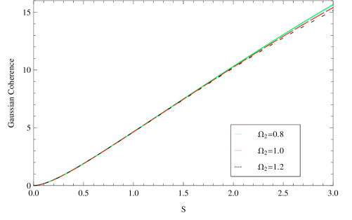
Figure 1: (Color online) The Gaussian coherence $C(\Sigma^{b_{1}b_{2}})$ as a function of the squeezing parameter $s$ for different peak frequencies, $\Omega_{2}=0.8$ (green solid line), $\Omega_{2}=1$ (red dashed line) and $\Omega_{2}=1.2$ (black dashed line), respectively. The orbit height of the satellite and the Gaussian bandwidth are fixed as $h=20000$ km and $\sigma=1$.

For convenience, we will work with dimensionless quantities by rescaling the peak frequency and the Gaussian bandwidth

$$\Omega\rightarrow\tilde{\Omega}\equiv\frac{\Omega}{\Omega_{B,0}},\sigma\rightarrow\tilde{\sigma}\equiv\frac{\sigma}{\sigma_{0}},$$ (25)

where $\Omega_{B,0}=500$THz and $\sigma_{0}=1$ MHz. For simplicity, we abbreviate the dimensionless parameter $\tilde{\Omega}$ as $\Omega_{2}$ and abbreviate $\tilde{\sigma}$ as $\sigma$, respectively.

To better understand the relation between Gaussian coherence and initial squeezing parameter. In Fig. (1) we plot the Gaussian coherence $C(\Sigma^{b_{1}b_{2}})$ as a function of the squeezing parameter $s$ for the fixed orbit height $h=20000$ km and Gaussian bandwidth $\sigma=1$. We can see that Gaussian coherence monotonically increases with the increase of the squeezing parameter $s$. We also can see that Gaussian coherence decreases with the growth of the peak frequency parameter of the mode $b_{2}$. However, comparing with the peak frequency parameter, Gaussian coherence $C(\Sigma^{b_{1}b_{2}})$ is easier effected by changing squeezing parameters. That is to say, the Gaussian coherence is more sensitive to squeezing parameter than peak frequency parameter.

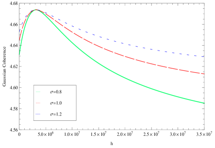
Figure 2: (Color online) The Gaussian coherence $C(\Sigma^{b_{1}b_{2}})$ in terms of the orbit height $h$ for different values of Gaussian bandwidth, $\sigma=0.8$ (green solid line), $\sigma=1$ (red dashed line) and $\sigma=1.2$ (blue dashed line), respectively. The squeezing parameter and peak frequency of mode $b_{2}$ are fixed as $s=1$ and $\Omega_{2}=1$.

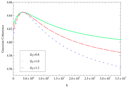
Figure 3: (Color online). The Gaussian coherence $C(\Sigma^{b_{1}b_{2}})$ in terms of the orbit height $h$ for different peak frequencies of mode $b_{2}$, $\Omega_{2}=0.8$ (green solid line), $\Omega_{2}=1$ (red dashed line) and $\Omega_{2}=1.2$ (blue dashed line), respectively. The other parameters are fixed as $s=1$ and $\sigma=1$.

The behavior of Gaussian coherence under the Earth’s gravitational field has been shown in Fig. (2) and (3). The Gaussian coherence $C(\Sigma^{b_{1}b_{2}})$ in terms of the orbit height $h$ with the different values of the Gaussian bandwidth has been shown in Fig. (2). Meanwhile, we plot the $C(\Sigma^{b_{1}b_{2}})$ in terms of the orbit height $h$ for different peak frequencies of mode $b_{2}$ in Fig. (3). Comparing these two pictures, we can see that the Gaussian coherence increases with the increase of Gaussian bandwidth parameter, but the Gaussian coherence decreases with the growth of the peak frequency. Moreover, the typical distance between the Earth and the geostationary satellite is about $3.6\times 10^{4}$ km, which yields the height $r_{B}=4.237\times 10^{4}$ km for the satellite. For this distance, the influence of relativistic disturbance of the spacetime curvature on quantum coherence cannot be ignored for the quantum information tasks at current level technology satellite1 ; satellite2 ; MJAG . Hence, we constrain the satellite height to geostationary Earth orbits $r_{B}(GEO)=r_{A}+3.6\times 10^{4}$ km.

The Fig. (2) and Fig. (3) both shown that Gaussian coherence increases for a specific range of height parameter $h\simeq\frac{r_{A}}{2}$ and then gradually approach to a finite value with increasing $h$. The physical support behind this is that the gravitational frequency shift effects would reduce quantum resource, but the special relativistic effects makes quantum resource growth. Since the special relativistic effects becomes smaller and smaller but the gravitational frequency shift can be cumulate with increasing height. The photon’s frequency received by satellites with height $h<\frac{r_{A}}{2}$ will experience blue-shift which cause Gaussian coherence increases, while the frequencies of photons received at height $h>\frac{r_{A}}{2}$ experience red-shift which cause Gaussian coherence decreases. In fact, the peak value of Gaussian coherence (the parameter $\delta=0$) indicates the fact that the photon’s frequency received by satellites experiences a transformation from blue-shift to red-shift, which causes the Gaussian coherence between the photon pairs to increase first and then to reduce with increasing height kerr . When two parties are situated at the same height or are in flat space-time, the parameter $\delta\neq 0$. It comes from the fact that we are expanding the total frequency shift in Eq. (10) taking into account both special and general relativistic effects kerr . When the satellite moves at the height $h=\frac{r_{A}}{2}$, the Schwarzschild term $\delta_{Sch}$ vanishes and photons received on satellites will generate a very small frequency shift effects, therefore the lowest order rotation term $\delta_{rot}$ needs to be considered. In addition, Gaussian coherence is not equal with different $\Omega_{2}$ and $\sigma$ when Alice and Bob at height $h=0$. The reason for this result is that $\delta\neq 0$ when height $h=0$, the contribution of the special relativity effects always existence which leads to $\Theta$ parameter is not equivalent to zero. And the parameter $\Theta$ not only depends on satellite’s height but also depends on Gaussian bandwidth parameter and peak frequency which means that different Gaussian bandwidth parameters and peak frequencies correspond to different $\Theta$ parameters.

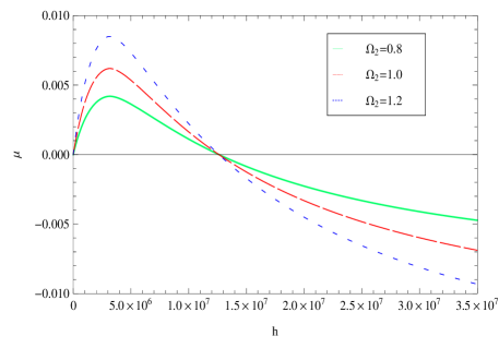
Figure 4: (Color online) The Gaussian coherence $C(\Sigma^{b_{1}b_{2}})$ in terms of the orbit height $h$ for different values of Gaussian bandwidth, $\sigma=0.8$ (green solid line), $\sigma=1$ (red dashed line) and $\sigma=1.2$ (blue dashed line), respectively. The squeezing parameter and peak frequency of mode $b_{2}$ are fixed as $s=1$ and $\Omega_{2}=1$.

Consider Gaussian coherence is a quantum resource, understanding how much Gaussian coherence affected by the Earth’s gravitational field is more important. We calculate the rate of change of Gaussian coherence $\mu$ according follow equation

$$\mu=\frac{C(\Sigma^{b_{1}b_{2}})-C_{0}(\Sigma^{b_{1}b_{2}})}{C_{0}(\Sigma^{b_{1}b_{2}})},$$ (26)

where $C_{0}(\Sigma^{b_{1}b_{2}})$ is value of Gaussian coherence $C(\Sigma^{b_{1}b_{2}})$ with the satellite’s height $h=0$, the parameter $\mu$ means the degree of change of Gaussian coherence suffers the Earth’s gravitational field. We shown the rate of change of Gaussian coherence $\mu$ for different peak frequencies $\Omega_{2}$ with the fixed $\sigma=1$ in Fig. (4). It is easy to see that value of $\mu$ increases when height parameter $h<\frac{r_{A}}{2}$, then gradually decreases, which indicates that the Earth’s gravitational effect for photon’s frequency shift is blue-shift in $h<\frac{r_{A}}{2}$ range, for $h>\frac{r_{A}}{2}$ range, is red shift. It is also shown that total gravitational frequency shift causes the change of Gaussian coherence less than $\%1$ with the satellite height in geostationary Earth orbits. In addition, the point $h=2r_{A}$ (i.e. the parameter $\delta=-1$) means that the Earth’s gravitational frequency shift for photon is no contribution, the blue-shift and the red-shift effect for photon’s frequency are offset, there’s only special relativity effect. The different initial peak frequencies also can effect rate of change $\mu$. This conclusion give us guide to choose appropriate physical parameters to constrains unnecessary loss of Gaussian coherence between the Earth to satellites.

V Conclusions

In conclusion, we have studied Gaussian coherence for a two-mode Gaussian state when one of the modes propagates from the ground to satellites. We found that the frequency shift induced by the curved spacetime of the Earth reduces the quantum correlation of coherence between the photon pairs when one of the entangled photons is sent to the Earth station and the other photon is sent to the satellite. We also found that Gaussian coherence is easier to change with the initial squeezing parameter than the gravitational effect and other parameters. Meanwhile, we found that Gaussian coherence increases with the increase of Gaussian bandwidth parameter, but the Gaussian coherence decreases with the growth of the peak frequency. In addition, the peak value is found to be a critical point which indicates the Gaussian coherence experiences the blue-shift transforms into the red-shift. Finally, it is also found that total gravitational frequency shift causes the change of Gaussian coherence less than $\%1$ and different initial peak frequencies also can effect rate of change with the satellite height in geostationary Earth orbits. According to the equivalence principle, the effects of acceleration are equivalence with the effects of gravity, our results could be in principle apply to dynamics of quantum coherence under the influence of acceleration. Since realistic quantum systems will always exhibit gravitational and relativistic features, our results should be significant both for giving more advices to realize quantum information protocols such as quantum key distribution from Earth to satellites and for a general understanding of quantum coherence in relativistic quantum systems.

- (1) A. J. Leggett, Prog. Theor. Phys. Suppl. 69, 80 (1980).
- (2) V. Giovannetti, S. Lloyd, and L. Maccone, Science. 306, 1330 (2004).
- (3) R. Demkowicz-Dobrzanski and L. Maccone, Phys. Rev. Lett. 113, 250801 (2014).
- (4) J. K. Asb th, J. Calsamiglia, and H. Ritsch, Phys. Rev. Lett. 94, 173602 (2005).
- (5) A. Streltsov, U. Singh, H. S. Dhar, M. N. Bera, and G. Adesso, Phys. Rev. Lett. 115, 020403 (2015).
- (6) R. J. Glauber, Phys. Rev. 131, 2766 (1963).
- (7) M. O. Scully, Phys. Rev. Lett. 67, 1855 (1991).
- (8) A. Albrecht, J. Mod. Opt. 41, 2467 (1994).
- (9) D. F. Walls and G. J. Milburn, Quantum Optics (Springer- Verlag, Berlin, 1995).
- (10) M. Nielsen and I. Chuang, Quantum Computation and Quantum Information (Cambridge University Press, Cambridge, England, 2000), ISBN: 9781139495486.
- (11) T. Baumgratz, M. Cramer, and M. B. Plenio, Phys. Rev. Lett. 113, 140401 (2014).
- (12) F. Levi and F. Mintert, New J. Phys. 16, 033007 (2014).
- (13) I. Marvian and R.W. Spekkens, New J. Phys. 15, 033001 (2013).
- (14) J. Åberg, arXiv:quant-ph/0612146 (2006).
- (15) S. D. Bartlett, T. Rudolph, and R.W. Spekkens, Rev. Mod. Phys. 79, 555 (2007).
- (16) I. Marvian, Ph.D. thesis, University of Waterloo, 2012.
- (17) D. Girolami, T. Tufarelli, and G. Adesso, Phys. Rev. Lett. 110, 240402 (2013).
- (18) I.Marvian and R.W. Spekkens, Nat.Commun. 5, 3821 (2014)
- (19) D. Girolami, Phys. Rev. Lett. 113, 170401 (2014).
- (20) D. Girolami, A. M. Souza, V. Giovannetti, T. Tufarelli, J. G. Filgueiras, R. S. Sarthour, D. O. Soares-Pinto, I. S. Oliveira, and G. Adesso, Phys. Rev. Lett. 112, 210401 (2014).
- (21) J. Aberg, Phys. Rev. Lett. 113, 150402 (2014).
- (22) S. Luo, S. Fu, and C. H. Oh, Phys. Rev. A. 85, 032117 (2012).
- (23) X. Yuan, H. Zhou, Z. Cao, and X. Ma, Phys. Rev. A. 92, 022124 (2015).
- (24) Z. Xi, Y. Li, and H. Fan, Sci. Rep. 5, 10922 (2015).
- (25) A.Winter and D. Yang, Phys. Rev. Lett. 116, 120404 (2016).
- (26) E. Chitambar, A. Streltsov, S. Rana, M. N. Bera, G. Adesso, and M. Lewenstein, Phys. Rev. Lett. 116, 070402 (2016).
- (27) D. Samos-Sàenz D. Buruaga, C. Sab, Phys. Rev. A. 95, 022307 (2017).
- (28) J. Wang, Z. Tian, J. Jing and H. Fan, Phys. Rev. A 93, 062105 (2016).
- (29) C. Chou, D. Hume, T. Rosenband, and D. Wineland, Science. 329, 1630 (2010).
- (30) J. Wang, Z. Tian, J. Jing, and H. Fan, Phys. Rev. D. 93, 065008 (2016).
- (31) M. Zych, F. Costa, I. Pikovski, and C. Brukner, Nat. Commun. 2, 505 (2011).
- (32) M. Ahmadi, D. Bruschi, and I. Fuentes, Phys. Rev. D. 89, 065028 (2014).
- (33) M. Ahmadi, D. Bruschi, C. Sabìn, G. Adesso, and I. Fuentes, Sci. Rep. 4, 4996 (2014).
- (34) S. Kish and T. Ralph, Phys. Rev. D. 93, 105013 (2016).
- (35) T. Liu, J. Jing, J. Wang, Adv. Q. T. 1, 2 (2018).
- (36) M. Nielsen and I. Chuang, Quantum computation and quantum information (Cambridge University Press, 2000).
- (37) P. Rohde, W. Mauerer, and C. Silberhorn, New J. Phys. 9, 91 (2007).
- (38) D. Bruschi, T. Ralph, I. Fuentes, T. Jennewein, and M. Razavi, Phys. Rev. D. 90, 045041 (2014).
- (39) M. Visser, arXiv:0706.0622 (2007).
- (40) U. Leonhardt, Measuring the Quantum State of Light, Cambridge Studies in Modern Optics (Cambridge University Press, Cambridge, 2005).
- (41) T. Downes, T. Ralph, and N. Walk, Phys. Rev. A. 87, 012327 (2013).
- (42) D. Bruschi, A. Datta, R. Ursin, T. Ralph, and I. Fuentes, Phys. Rev. D. 90, 124001 (2014).
- (43) C. Weedbrook, S. Pirandola, R. García-Patrón, N. J. Cerf, T. C. Ralph, J. H. Shapiro, and S. Lloyd, Rev. Mod. Phys. 84, 621 (2012).
- (44) R. Simon, Phys. Rev. Lett. 84, 2726 (2000).
- (45) L.-M. Duan, G. Giedke, J. I. Cirac, and P. Zoller, Phys. Rev. Lett. 84, 2722 (2000).
- (46) D. Buono, G. Nocerino, A. Porzio, and S. Solimeno, Phys. Rev. A. 86, 042308 (2012).
- (47) F. A. S. Barbosa, A. J. de Faria, A. S. Coelho, K. N. Cassemiro, A. S. Villar, P. Nussenzveig, and M. Martinelli, Phys. Rev. A. 84, 052330 (2011).
- (48) J. W. Xu, Phys.Rev. A. 93, 032111 (2016).
- (49) A. S. Holevo, M. Sohma, and O. Hirota, Phys. Rev. A. 59, 1820 (1999).
- (50) M. Razavi and J. Shapiro, Phys. Rev. A. 73, 042303 (2006).
- (51) D. Matsukevich, P. Maunz, D. Moehring, S. Olmschenk, and C. Monroe, Phys. Rev. Lett. 100, 150404 (2008).
- (52) G. Vallone, D. Bacco, D. Dequal, S. Gaiarin, V. Luceri, G. Bianco, and P. Villoresi, Phys. Rev. Lett. 115, 040502 (2015).
- (53) J. Yin et. al, Science. 356, 1140 (2017).
- (54) M. Jofre, A. Gardelein, G. Anzolin, W. Amaya, J. Capmany, R. Ursin, L. Penate, D. Lopez, J. Juan, J. Carrasco, Opt. Express 19, 3825 (2011).
- (55) J. Kohlrus, D. Bruschi, J. Louko, and I. Fuentes, EPJ Quantum Technology. 4, 7 (2017).