Abstract

This study provided a model for the publication dynamics of researchers, which is based on the relationship between the publication productivity of researchers and two covariates: time and historical publication quantity. The relationship allows to estimate the latent variable the publication creativity of researchers. The variable is applied to the prediction of publication productivity for researchers. The statistical significance of the relationship is validated by the high quality dblp dataset. The effectiveness of the model is testified on the dataset by the fine fittings on the quantitative distribution of researchers’ publications, the evolutionary trend of their publication productivity, and the occurrence of publication events. Due to its nature of regression, the model has the potential to be extended for assessing the confidence level of prediction results, and thus has applicability to empirical research.

Keywords: Scientific publication, Productivity prediction, Data modelling.

Introduction

Predicting the scientific success of researchers is a topic in the scientific fields such as informetrics, scientometrics, and bibliometrics[1]. It has three main aspects: the $h$-index[2], citation-based indexes, and publication productivity. Much attention on this topic has concentrated on the $h$-index: the maximum value of $h$ such that a researcher has produced $h$ publications that have each been cited at least $h$ times. The popularity of the $h$-index is attributable to its simplicity and its addressing both the productivity and the citation impact of publications[3]. Acuna et al presented a prediction formula to show that the current $h$-index is the most significant predictor, compared with the number of current papers, the year since publishing first paper, etc[4]. Mccarty et al showed that the number of coauthors and their $h$-index also are significant predictors[5]. The formula provided by Dong et al utilized more features, such as the average citations of an author’s papers, and the number of coauthors[6].

Predicting highly cited publications by short-term citation data also attracts considerable attention. Mazloumian applied a multi-level regression model[7]; Wang et al derived a mechanistic model[8]; Newman defined $z$-scores[9]; Gao et al utilized a Gaussian mixture model[10]; Pobiedina applied link prediction[11]; Abrishami et al utilized deep learning[12]. More information of publications (such as journal, authors, and content) has been utilized to improve prediction precision: Bornmann et al considered publications’ length[13]; Sarigol et al used specific characteristics of coauthorship networks[14]; Yu et al synthesized the features of publications, authors, and journals[15]; Klimek et al utilized the centrality measures of term-document networks[16]; Kosteas considered the rankings of journals[17], Bai et al used the aging of publications’ impact[18]; Stern and Abramo utilized the impact factors of journals[20, 19].

Fewer attention has concentrated on the prediction of publication productivity, compared with that on $h$-index and citation-based indexes. Empirical studies found the cumulative advantage in producing publications and the aging of researchers’ creativity[21, 22]. Laurance et al found that Pre-PhD publication success strongly correlates to long-term success[23]. Lehman concluded that productivity usually begins in a researcher’s 20s, rises sharply to a peak in the late 30s or early 40s, and then declines slowly[24]. In the year 1984, Simonton provided a formula to model this process[25], which, however, is at variance with the observations on the vast numbers of current researchers.

Aforementioned prediction methods of citation-based indexes and $h$-index all refer to the positive correlation between the current indexes and their historical quantity. The current $h$-index, the number of annual citations, and the number of five-year citations are found to be their positive predictors. The success of those methods can be thought to result from the cumulative advantage of receiving citations found by Price in the year 1965[26], which has been extended as a general theory for bibliometric and other cumulative advantage process[27, 28, 29]. From the perspective of statistics, the success is due to the predictable components of these indicators that can be extracted via autoregression.

The effect of cumulative advantage in producing publications is weaker than that in receiving citations. It is displayed as that the tail of the quantitative distribution of the publications produced by a group of researchers is much shorter than that of the citation distribution of those researchers[30]. Therefore, the critical factor of the success in the prediction of citation-based indexes and the $h$-index does not exist in the prediction of publication productivity. Then, is there still any predictability in publication patterns?

We provided a model to estimate the latent variable the creativity of researchers on publications, termed publication creativity, through an observed variable publication productivity. Given a group of researchers, the quantitative distribution of their publications can be thought as a mixture of Poisson distributions[31, 32, 33, 34]. Samples following the same Poisson distribution means that they would be drawn from the same population. It means researchers can be partitioned into several populations, each of which has certain homogeneity in publication patterns. And the publication creativity of each subset of the partition can be regarded as the expected value of the corresponding Poisson distribution. Therefore, finding such a partition will contribute to revealing the mystery of publication patterns.

We used a partition scheme, such that each subset consists of the researchers with the same number of historical publications produced before the current time. When applying to the dblp dataset, we found that for the majority of researchers, the scheme satisfies our requirement. Furthermore, we found that researchers’ publication productivity significantly correlates to time given a quantity of historical publications, and to researchers’ historical publication quantity given a time. It allows us to estimate researchers’ publication creativity at each time interval, and then to infer their productivity in the future. Three methods are provided to test the prediction results of our model in terms of the evolutionary trend of productivity, the quantitative distribution of publications, and the occurrence of publication events. Compared with the model in the previous work[35], the model removes the limitation on the prediction for high productive researchers, however, its precision still needs to be improved. In addition, the model decreases the requirement of training dataset on the quantity of productive researchers.

This paper is organized as follows. The model and its motivation are described in Sections 2, 3. The empirical data and experiments are described in Section 4. The results are discussed and conclusions drawn in Section 5.

Motivation

Latent publication creativity

Finding regularities in the publication patterns of researchers is an elusive task. Several factors on individual level have been used to explain the productivity levels among researchers, such as work habits, psychological traits (intelligence, creativity, etc.), demographic characteristics (aging, gender, etc.), and environmental location (graduate school background, the prestige of institution, etc.)[36]. Many of these investigations focused on the psychological traits. For example, Andrews reported that creativity may not result in productivity unless the researchers have strong motivations[37]. Our study considers the creativity on producing publications, termed “publication creativity”.

A latent variable model contains latent variables that cannot be directly observed. Those variables have connections to certain variables that can be observed directly. The annual publication creativity of a researcher is such an unobserved variable. The provided model gives a method to measure it as the expected value of an observed variable the annual publication productivity of researchers. The publication productivity of a researcher is easily affected by random factors from his or her work environment, family, etc. Meanwhile, its expected value could be relatively stable, which would be more suitable for the prediction of publication quantity.

Inhomogeneous Poisson process

How to define the publication creativity of researchers, and how to calculate it based on empirical data? The definition given here is based on the feature of the quantitative distributions of researchers’ publications. These distributions can be fitted by a mixture of Poisson distributions[34]. Therefore, we could expect to partition researchers into specific subsets, such that the distribution of each subset is a Poisson distribution. In this study, the publication creativity of any researcher in the subset is defined to be the expected value of the Poisson distribution. The publication productivity of the researcher is treated as a sample from the distribution; thus has certain randomness.

How to find those subsets? Previous studies show that the distributions are featured by a trichotomy, comprising a generalized Poisson head, a power-law middle part, and an exponential cutoff[38]. The trichotomy can be derived from a range of “coin flipping” behaviors, where the probability of observing “head” is dependent on observed events [39]. The event of producing a publication can be regarded as an analogy of observing “head”, where the probability of publishing is also affected by previous events. Researchers would easily produce their later publications, compared with their first one. This is a cumulative advantage, research experiences accumulating in the process of producing publications. It displays as the transition from the generated Poisson head to the power-law part. Aging of researchers’ creativity is against cumulative advantage, displaying as the transition from the power-law part to the exponential cutoff.

When considering a short time interval, the effects of cumulative advantage and aging would be not significant. However, the diversity of researchers in publication history cannot be eliminated only by shrinking the observation window in the time dimension. Therefore, we partitioned researchers into $I$ subsets, where $I$ is a given integer. For $i=1,2,...,I$, the $i$-th subset contains the researchers with $i$ historical publications before the current time. In practice, the historical publications are counted since a given time $T_{0}$.

The Lotka’s law

Lotka analyzed the publications of physics journals during the nineteenth century, and found the law: the publication quantity of a researcher approximately satisfies that the number producing $n$ (where $n\in\mathrm{Z}^{+}$) publications is about $1/n^{2}$ of those producing one[40]. It is named Lotka’s law and stimulates Price’s study on the patterns of long-term historical publications. Price provided his “inverse square law” that half of the publications come from the square root of all researchers[41].

Lotka’s law is now usually defined in the generalized form $p(x=h)\propto h^{a}$, where $a<-1$, $h\in\mathbb{Z}$, $x$ is random variable, and $p(x=h)$ represents the probability that a researcher produced $h$ publications. Therefore, given a set of researchers, the probability of a researcher with $s$ publications at time interval $[T_{0},T_{1}]$ can be supposed to be proportional to $s^{a}$. Assume that the researcher’s publication productivity at a following time interval $(T_{1},T_{2}]$ is $s^{b}$, where $b>0$. It gives rise to $p(x=s^{b})\propto s^{a}$ at time interval $(T_{1},T_{2}]$. Letting $h=s^{b}$ obtains $p(x=h)\propto h^{a/b}$. Therefore, with the assumption, the Lotka’s law holds at the following time interval. It gives certain reasonability to the assumption, which is needed by the log-log regression of the model.

The model

Model terms

Consider the researchers who produced publications at two time intervals $[T_{0},T_{1}]$ and $[T_{1},T_{2}]$. Our aim is to estimate researchers’ publication creativity at $[T_{1},T_{2}]$. Partition $[T_{1},T_{2}]$ into $J$ intervals with cutpoints $T_{1}=t_{0}<t_{1}<\cdots<t_{J}=T_{2}$. The half-closed interval $(t_{j-1},t_{j}]$ is referred to as the $j$-th time interval, where $j=1,2,...,J$. Partition the researchers with no more than $I$ publications at $[T_{0},t_{j}]$ into $I$ subsets according to their historical publication quantity at $[T_{0},t_{j-1}]$. That is, the $i$-th subset consists of the researchers with $i$ publications at $[T_{0},t_{j-1}]$.

Let the $i$-th subset at the $j$-th time interval be the subset of the researchers with $i$ publications at $[T_{0},t_{j-1}]$. Define the publication productivity of the $i$-th subset in the dataset at $(t_{j-1},t_{j}]$ to be the average publication quantity of its researchers at that time interval, and denote it by $\eta_{ij}$. It can be calculated as follows:

$$\eta_{ij}=\frac{m_{ij}}{n_{ij}},$$ (1)

where $n_{ij}$ is the number of researchers with $i$ publications at $[T_{0},t_{j-1}]$, and $m_{ij}$ is the number of publications produced by those researchers at $(t_{j-1},t_{j}]$. Define the publication creativity of the $i$-th subset at the $j$-th time interval to be the expected value of $\eta_{ij}$, and denote it by $\lambda_{ij}$.

Regression formulae

The provide model is the combination of a piecewise Poisson regression and a log-log regression. Firstly, treating the index $i$ of $\lambda_{ij}$ as a dummy index, we assumed $\lambda_{i1}>0$ and

$$\lambda_{ij}=\lambda_{i1}\mathrm{e}^{{\beta_{i}}({t}_{j}-t_{1})},$$ (2)

where $\beta_{i}$ tunes the effect of ${t}_{j}$. The proportionate $\mathrm{e}^{{\beta}_{i}{t}_{j}}$ changes the creativity. Taking logs in Eq. (2) obtains

$$\log\lambda_{ij}=\alpha_{i}+\beta_{i}(t_{j}-t_{1}),$$ (3)

where $\alpha_{i}=\log\lambda_{i1}$. For each subset $i$, Eq. (3) is a one-variable Poisson model (see its definition in Appendix A). Because for the majority of researchers in any subset $i$, their number of publications produced at a short time interval (e. g. a year) follows a Poisson distribution[35].

Secondly, treating the index $j$ of $\lambda_{ij}$ as a dummy index, we assumed $\lambda_{1j}>0$ and

$$\lambda_{ij}=\lambda_{1j}i^{\nu_{j}},$$ (4)

where $\nu_{j}$ tunes the effect of $i$. Taking logs in Eq. (4) obtains

$$\log\lambda_{ij}=\mu_{j}+\nu_{j}\log i,$$ (5)

where $\mu_{j}=\log\lambda_{1j}$, and $\lambda_{1j}>0$ for empirical data. Therefore, for each time interval, Eq. (5) is a one-variable log-log model (see its definition in Appendix A).

Except for the Poisson feature of empirical distributions of researchers’ publications and the Lotka’s law, the reasonability of the assumptions of the regression formulae in Eqs. (3) and (5) are also based on the significant relationship between covariates and response variables found in empirical data. Note that the regression formulae can be generalized to deal several characteristics varying with $i$ and $j$. This study only considered the simplest case: one characteristic for each index.

Training process

Consider a training dataset consisting of the researchers producing publications at the time interval $[T_{0},t_{L-1}]$ and their publications at the time interval $[T_{0},t_{L}]$, where $L$ is an integer larger than $1$. At each time $t_{l}$ ($0<l<L$), we considered the researchers of the training dataset, whose publication quantity at $[T_{0},t_{l-1}]$ is no more than a given integer $K$. Partition these researchers into $K$ subsets according to their publication quantity at $[T_{0},t_{l-1}]$. The training dataset is utilized to calculate $m_{ij}$ and $n_{ij}$, namely the publication productivity $\eta_{ij}$. The publication creativity can be expressed by a matrix $(\lambda_{ij})_{I\times J}$. To show its computational process clearly, we divided the matrix into four zones (Fig. 1).

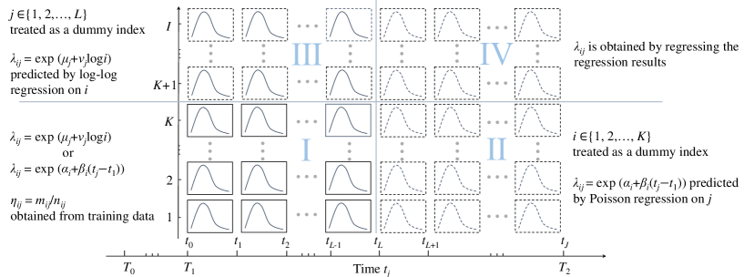
Figure 1: An illustration of the latent model. The publication productivity $\eta_{ij}$ in Zone I is calculated based on the training dataset. The matrix of publication creativity $(\lambda_{ij})_{I\times J}$ is divided into four zones, which is calculated by the approach shown in Section 3.

Firstly, we replaced the $\lambda_{ij}$ in Eq. (3) by $\eta_{ij}$, and obtained

$$\log\eta_{ij}=\alpha_{i}+\beta_{i}(t_{j}-t_{1}).$$ (6)

Utilize the linear regression to calculate $\alpha_{i}$ and $\beta_{i}$ for $i=1,...,K$. Let $\lambda_{ij}=\mathrm{e}^{\alpha_{i}+\beta_{i}(t_{j}-t_{1})}$, where $j=1,...,J$. It values the $\lambda_{ij}$ in Zones I and II.

Secondly, we replaced the $\lambda_{ij}$ in Eq. (5) by $\eta_{ij}$, and obtained

$$\log{\eta_{ij}}=\mu_{j}+\nu_{j}i.$$ (7)

Utilize the linear regression to calculate $\mu_{j}$ and $\nu_{j}$ for $j=1,...,L$. Let $\lambda_{ij}=\mathrm{e}^{\mu_{j}}i^{\nu_{j}}$, where $i=1,...,I$. It values the $\lambda_{ij}$ in Zones I and III.

Thirdly, we substituted the calculated $\lambda_{ij}$ in Zone III into Eq. (3), and utilized the linear regression to calculate $\alpha_{i}$ and $\beta_{i}$ for $i=K+1,...,I$. Let $\lambda_{ij}=\mathrm{e}^{\alpha_{i}+\beta_{i}(t_{j}-t_{1})}$, where $j=L+1,...,J$. It values the $\lambda_{ij}$ in Zone IV. We can also substitute the calculated $\lambda_{ij}$ in Zone II into Eq. (5), and utilized the linear regression to calculate $\mu_{j}$ and $\nu_{j}$ for $j=L+1,...,J$. Let $\lambda_{ij}=\mathrm{e}^{\mu_{j}}i^{\nu_{j}}$, where $i=K+1,...,I$. It also values the $\lambda_{ij}$ in Zone IV.

Note that the production creativity $\lambda_{ij}$ in Zones I and IV has two values. For the majority researchers of the training dataset used in the next section, we found that $\eta_{ij}$ significantly correlates to $t_{j}$ given $i$ and to $i$ given $t_{j}$. Therefore, either the two values of $\lambda_{ij}$ or their average can be used due to the statistical significance of regression.

Predicting publication quantity

Algorithm 1 is provided to predict researchers’ publication quantity at the time interval $[t_{X},t_{Y}]$, where $t_{0}\leq t_{X}<t_{Y}\leq t_{J}$. Denote the publication quantity of researcher $s$ at $[T_{0},t_{l}]$ by $h_{s}(t_{l})$. The algorithm gives $h_{s}(t_{Y})$ the predicted publication quantity of researcher $s$ at $[T_{0},t_{Y}]$. Due to its regression nature, the algorithm cannot exactly predict the publication quantity for an individual, but it can be suitable for a group of researchers.

Note that the training dataset would contain not enough productive researchers. It would cause the parameter $K$ much smaller than the largest publication quantity $I$ that can be predicted by our model. In this case, the model will give bad prediction results to productive researchers.

Algorithm 1 Predicting researchers’ publication quantity.

0:    the $h_{s}(t_{X})$ of any researcher $s$ in a test dataset; the publication creativity matrix $(\lambda_{ij})_{I\times J}$.

0:    the predicted productivity $h_{s}(t_{Y})$ of researcher $s$.

  for each researcher $s$ do

     initialize $h=h_{s}(t_{X})$;

     for $l$ from ${X+1}$ to $Y$ do

        sample an integer $r$ from $\mathrm{Pois}(\lambda_{hl})$;

        let $h=h+r$;

     end for

     let $h_{s}(t_{Y})=h$;

  end for

Experiments

Empirical data

To guarantee the prediction precision of the provided model, we need a large training dataset, which should contain enough productive researchers. The dataset provided by the dblp computer science bibliography satisfies our requirement, which consists of the open bibliographic information on the major journals and proceedings of computer science (https://dblp.org). The dataset is of high quality, because it has been corrected by several methods of name disambiguation and checked manually.

To show the improvement of the provided model, we used the some training and test datasets used in Reference[35] (see Table 1). Sets 1 and 2 are used to extract the historical publication quantity for the test researchers in Sets 3 and 4. Sets 5 are 6 are used as training datasets. Sets 7 and 8 are used to testify the prediction results for the researchers in Sets 3 and 4. These datasets consist of 220,344 publications in 1,586 journals and proceedings, which are produced by 328,690 researchers at the years from 1951 to 2018. Due to the size and time span of the analyzed datasets, our model is at least suitable for the community of computer science.

Table 1: Certain subsets of the dblp dataset.

Dataset	$a$	$b$	$c$	$d$	$e$	$f$
Set 1	1951–1994	180,45	18,398	319	1.558	1.528
Set 2	1951–2000	38,149	35,643	542	1.571	1.681
Set 3	1994	2,903	1,922	146	1.137	1.718
Set 4	2000	5,741	3,600	257	1.184	1.888
Set 5	1994–2009	88,853	64,558	940	1.545	2.126
Set 6	1995–2009	87,140	62,636	931	1.538	2.139
Set 7	1995–2018	316,212	201,946	1,538	1.754	2.746
Set 8	2001–2018	301,741	184,701	1,495	1.733	2.831

The index $a$: the time interval of data, $b$: the number of researchers, $c$: the number of publications, $d$: the number of journals, $e$: the average number of researchers’ publications, $f$: the average number of publications’ authors.

In this section, Set 6 is used as the training dataset. Its parameters are $I=180$, $J=23$, $K=42$, $L=14$, $T_{0}=1951$, $T_{1}=t_{0}=1995$, $t_{L}=2009$, and $t_{J}=T_{2}=2018$. The test dataset here consists of the researchers in Set 4, their historical publication quantity from Set 2, and their annual publication quantity from Set 8. Its parameters are $t_{X}=2000$, and $t_{Y}=2018$.

The publication productivity matrix $(m_{ij}/n_{ij})_{K\times L}$ is calculated based on the training dataset. For example, $n_{11}$ is the number of researchers with one publication at $1[951,1995]$, and $m_{11}$ is publication quantity of those researchers at the year $1996$. The publication creativity matrix $(\lambda_{ij})_{I\times J}$ is calculated by the method described in Section 3.

We predicted the publication quantity only for 99.98% test researchers who have no more than $I_{1}=60$ publications at the time interval $[1951,2000]$. Note that their predicted publication quantity can be more than $K=42$. That is, the model here removes a limitation of the model in Reference[35]: the upper limit of predicting output controlled by the parameter $K$.

The reasonability of model assumptions

Firstly, we showed the Poisson nature of the quantitative distributions of researchers’ publications. Consider the researchers of the training dataset who have publications at the year $y$ and no more than 10 publications at $[1951,y]$, where $y=1995,...,2018$. Consider the quantitative distributions of their publications produced at $y+1$. The Kolmogorov-Smirnov (KS) test rejects to regard some of them as Poisson distributions because of their tail (Fig. 2).

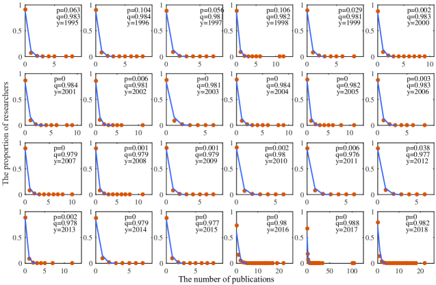
Figure 2: The quantitative distribution of researchers’ publications. Consider the researchers who produced publications at the year $y$ and no more than 10 publications at $[1951,y]$. Index $q$ is their proportion to the total researchers who produced publications at $y$. When $p<0.05$, the KS test rejects that the quantitative distribution of the publications produced by the considered researchers at the year $y+1$ (red circles) is a Poisson (blue lines).

Consider the researchers of the training dataset who have publications at the year $y$ and $i$ publications at $[1951,y]$. Fig. 3 shows that the quantitative distribution of their publications produced at $y+1$ is a Poisson, where $y=2001,...,2015$. That is, diminishing the diversity in researchers’ historical publication quantity can reveal the Poisson nature of the quantitative distributions of researchers’ publications.

There emerges a fraction of very productive researchers at the year from 2016 to 2018. A few of them even produced more than 100 publications a year, although their historical publication quantity is no more than 20. Consider the researchers who produced publications at $y$ and no more than 6 publications at $y+1$. Partition them into subsets according to their historical publication quantity at $[1951,y]$. For some subsets of these researchers, their publication distribution is still a Poisson (Fig. 4). It indicates that the partition is suitable to calculate publication creativity for the majority of researchers (see the proportion $q$ in Fig. 4); thus the principle of model still holds for those researchers.

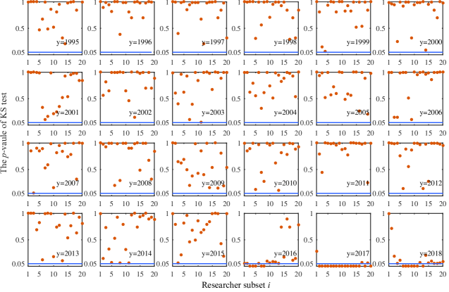
Figure 3: Eliminating the diversity in researchers’ historical publication quantity induces Poisson distributions. Consider the researchers who produced publications at $y$ and $i$ publications at $[1951,y]$. When the $p$-value$>0.05$, the KS test cannot reject that the quantitative distribution of the publications produced by these researchers at $y+1$ is a Poisson.

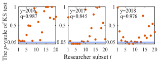
Figure 4: Poisson feature holds for the majority of researchers. The $p$-value is that of the KS test in the caption of Fig 3 on the researchers who produced $i$ publications at $[1951,y]$, publications at $y$, and no more than $6$ publications at $y+1$. Index $q$ is proportion of the researchers who passed the test.

Secondly, we showed the significance of regression results on the training dataset. The $\chi^{2}$ test indicates that publication productivity significantly correlates to time given a historical publication quantity$\leq 12$ (see the $p$-values in Fig. 5). That is, the significance holds for $99.61\%$ researchers in the training dataset. The $\chi^{2}$ test indicates that publication productivity significantly correlates to historical publication quantity given a time (see the $p$-values in Fig. 6). The significance holds for all of the researchers in the training dataset. Those guarantee the effectiveness of calculating $(\lambda_{ij})_{I\times J}$ by regression.

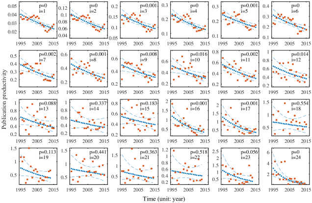
Figure 5: The relationship between publication productivity and time. Consider the subset of the researchers who have $i$ publications at $[1951,y]$. Panels show its publication productivity at $y+1$ (red squares), its predicted productivity by the Poisson model (blue dots), and the confidence intervals of regression (dashed lines). The relationship is significant, when $p<0.05$.

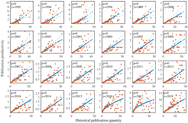
Figure 6: The relationship between publication productivity and historical publication quantity. Consider the subset of the researchers who have $i$ publications at $[1951,y]$. Panels show its productivity at the year $y+1$ (red squares), its predicted productivity by the log-log model (blue dots), and the confidence intervals of regression (dashed lines). When $p<0.05$, the relationship is significant.

Predicting the evolutionary trend of publication quantity

Consider the test researchers who produced $i$ publications at $[1951,2000]$. Let $n(i,y)$ be the average number of publications produced by these researchers at $[1951,y]$, and $m(i,y)$ be the predicted one. Fig. 7 shows their trend about $i$ given $y$. The correlation between them is measured by the Pearson correlation coefficient[42] on individual level ($s_{1}$) and that on group level ($s_{2}$). Index $s_{1}$ decreases over time, whereas $s_{2}$ keeps high. It indicates that the model is unapplicable to the long-time prediction for an individual, but can be applicable for a group of researchers.

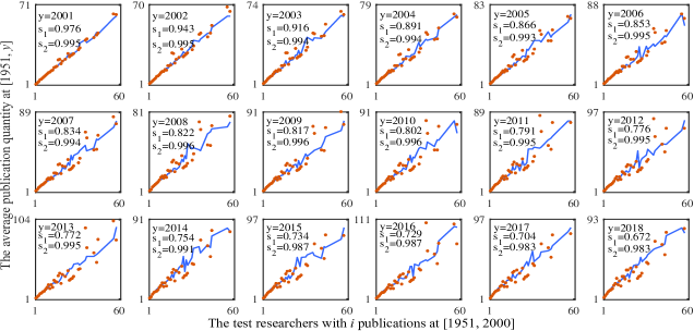
Figure 7: Fittings on the evolutionary trend of researchers’ publication quantity. Consider the test researchers who have $i$ publications at $[1951,2000]$. Panels show the average number of publications produced by these researchers at $[1951,y]$ ($n(i,y)$, red dots) and the predicted one ($m(i,y)$, blue lines). Index $s_{1}$ is the Pearson correlation coefficient calculated based on the list of researchers’ publication quantity and that of their predicted one. Index $s_{2}$ is that based on the sorted lists.

Predicting quantitative distributions of publications

We compared the distribution for the publications produced by the test researchers at $[T_{0},y]$ with the predicted one, where $y=2001,...,2018$. Fig. 8 shows that a fat tail emerges in the evolution of the ground-truth distribution and in that of the predicted one. It shows that our model can capture the fat-tail phenomenon. Meanwhile, the predicted quantity of the model in Reference[35] cannot be larger than the parameter $K$. However, when the time grows, the KS test still rejects that the compared distributions are the same (see the $p$-values in Fig. 8), although there is a coincidence in their forepart. It indicates that the prediction precision for productive researchers still needs to be improved.

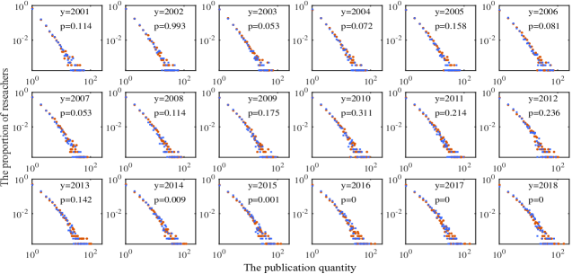
Figure 8: Fittings on the quantitative distribution of researchers’ publications. Panels show the quantitative distribution of the publications produced by the test researchers at $[1951,y]$ (red circles) and the predicted one (blue squares). When $p>0.05$, the KS test cannot reject the hypothesis that the compared distributions are the same.

Predicting publication events

The model gives the publication creativity $\lambda_{ij}$ to the $i$-th subset at the $j$-th time interval. It can be used to calculate $1-\mathrm{e}^{-\lambda_{ij}}$ the probability of a test researcher (who has $i$ publications at $[T_{0},t_{j-1}]$) producing publications at $(t_{j-1},t_{j}]$. The area under the receiver operating characteristic curve (AUC) is used to measure the prediction precision on publication events.

Count the times when a researcher who did (did not) produce publications at the next time interval and the probability is larger (smaller) than 0.5, and denote the count by $m_{1}$. Count the times when the probability is 0.5, and denote the count by $m_{2}$. Denote the number of tested researchers by $m$. Index AUC is calculated as follows:

$$\mathrm{AUC}=\frac{m_{1}+0.5m_{2}}{m}.$$ (8)

Different from above two experiments focusing on the prediction precision at a long time interval, this experiment is designed to measure the precision at a short time interval, namely the next time interval. Fig. 9 shows that index AUC is high on the researchers with a small historical publication quantity $i$, which indicates the high precision of predicting publication events for low productive researchers. It also shows there is no regularity can be revealed by the model for productive researchers, which gives the improving direction of the model. Due to the vast number of low productive researchers, the value of AUC is high on all of the test researchers.

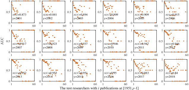
Figure 9: The precision of predicting publication events. Consider the test researchers who produced $i$ publications at $[1951,y-1]$. Panels show the AUC calculated by the formula in Eq. (8), which is the precision of predicting the publication events at the year $y$ for these researchers (red dots). Index AUC is calculated based on all of the test researchers.

Discussion and conclusions

We provided a model to estimate the publication creativity of researchers based on the relationship between publication productivity and two covariates, namely time and historical publication quantity. The model offers convincing evidence that the publication patterns of the majority of researchers are characterized by a piecewise Poisson process. Albeit simple, the model could be specified such that the creativity can be formulated as a function of time and the number of historical publications with the coefficients estimated from data, indicating the degree to which there is predictability.

The model is used to predict the publication quantities of the researchers in the dblp dataset. Its predictability is testified by the fine fittings on the evolutionary trend of researchers’ productivity, the quantitative distribution of their publications, and the probability of producing publications. Compared with the model in Reference[35], our model removes the limitation on predicting high productivity by using the log-log regression to estimate the publication creativity of productive researchers, and thus decreases the requirement of training dataset on the quantity of productive researchers.

Even where it does not provide an exact productivity prediction for individuals, especially for productive researchers, our model may still be of use in its ability to provide a satisfactory prediction for a group of researchers on average. Therefore, its prediction results offer some comfort: for an individual, rejecting a paper may feel indiscriminate and unfair, but for a group, these factors seem to average out. In addition, due to its advantage of providing results in an unbiased way, our model can be useful for funding agencies to evaluate the possibility of completing the quantitative index of publications in applications.

Phenomena studied in human behaviors are usually quite complex. Yet, little is known about the mechanisms governing the evolution of researchers’ publication productivity, whilst our model renders evolution trajectories relatively predictable on average. Predicting the productivity of productive researchers individually would not be done only by regression as this study did for a group of researchers, due to the randomness of an individual’s research. Analyzing massive data to track scientific careers would help to advance our understanding of how researchers’ productivity evolves. Therefore, advanced algorithms are needed to synthetically analyze the features extracted from researchers’ historical publications, eduction background, and published journals. Especially, we should consider the network features of their coauthorship (degree, betweenness, centrality, etc.), because previous studies showed that research collaboration contributes to scientific productivity[43, 44, 45].

Appendix A: the Poisson and log-log models

The Poisson model with one covariate is a generalized linear model of regression analysis[46]. It is used to model count data and contingency tables, thus has potential to predict publication productivity. It assumes that the response variable $y$ follows a Poisson distribution, and that the logarithm of its expected value can be expressed by a linear function of the covariate. Let ${x}\in\mathbb{R}$ be a covariate, and $\beta\in\mathbb{R}$ be the effect thereof. The Poisson model takes the form

$${\log({\mathbb{E}}(y|{x}))=\alpha+\beta{x}},$$ (9)

where $\alpha\in\mathbb{R}$, and ${\mathbb{E}}(y|{x})$ is the conditional expected value of $y$ given ${x}$.

The log-log model with one covariate assumes that the logarithm of its expected value can be expressed by a linear function of the logarithm of the covariate. The model takes the form

$${\log({\mathbb{E}}(y|{x}))=\alpha+\beta\log{x}}.$$ (10)

Appendix B: An other example

For the experiment of this section, Set 5 is used as a training dataset. Its parameters are $I=180$, $J=24$, $K=42$, $L=15$, $T_{0}=1951$, $T_{1}=t_{0}=1994$, $t_{L}=2009$, and $t_{J}=T_{2}=2018$. The test dataset here consists of the researchers from Set 3, their historical publication quantity from Set 1, and their annual publication quantity in Set 7. Its parameters are $t_{X}=1994$, and $t_{Y}=2018$. We only predicted the publications for 99.98% test researchers who have no more than $60$ publications at the time interval $[T_{0},T_{1}]$. Figs. 10-12 show the results of the test methods in Section 3.

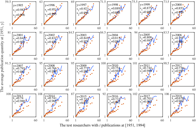
Figure 10: Fittings on the evolutionary trend of researchers’ publication quantity. Consider the test researchers who have $i$ publications at $[1951,1994]$. Panels show the average number of publications produced by these researchers at $[1951,y]$ ($n(i,y)$, red dots) and the predicted one ($m(i,y)$, blue lines). Index $s_{1}$ is the Pearson correlation coefficient calculated based on the list of researchers’ publication quantity and that of their predicted one. Index $s_{2}$ is that based on the sorted lists.

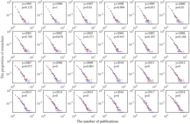
Figure 11: Fittings on the quantitative distribution of researchers’ publications. Panels show the quantitative distribution of the publications produced by the test researchers at $[1951,y]$ (red circles) and the predicted one (blue squares). When $p>0.05$, the KS test cannot reject the hypothesis that the compared distributions are the same.

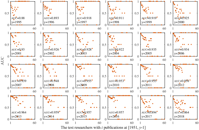
Figure 12: The precision of predicting publication events. Consider the test researchers who produced $i$ publications at $[1951,y-1]$. Panels show the AUC calculated by the formula in Eq. (8), which is the precision of predicting the publication events at $y$ for these researchers (red dots). Index AUC is calculated based on all of the test researchers.

References

- 1. Sinatra R, Wang D, Deville P, Song C, Barabási AL (2016) Quantifying the evolution of individual scientific impact. Science, 354(6312), aaf5239
- 2. Hirsch JE (2005) An index to quantify an individual’s scientific research output. Proc Natl Acad Sci USA 102, 16569-16572.
- 3. Schubert A (2007) Successive -indices. Scientometrics, 70, 201-205.
- 4. Acuna DE, Allesina S, Kording KP (2012) Future impact: Predicting scientific success. Nature, 489(7415), 201.
- 5. Mccarty C, Jawitz JW, Hopkins A, Goldman A (2013) Predicting author h-index using characteristics of the co-author network. Scientometrics, 96(2), 467-483.
- 6. Dong Y, Johnson RA, Chawla NV (2016) Can scientific impact be predicted? IEEE Transactions on Big Data, 2(1), 18-30.
- 7. Mazloumian A (2012) Predicting researchers’ scientific impact. Plos One, 7(11), 1-5.
- 8. Wang D, Song C, Barabási AL (2013) Quantifying long-term scientific impact. Science, 342(6154), 127-132.
- 9. Newman MEJ (2014) Prediction of highly cited papers. Europhys Lett, 105(2), 28002.
- 10. Cao X, Chen Y, Liu KR (2016) A data analytic approach to quantifying scientific impact. J Informetr, 10(2), 471-484.
- 11. Pobiedina N, Ichise R (2016) Citation count prediction as a link prediction problem. Appl Intell, 44(2), 252-268.
- 12. Abrishami A, Aliakbary S (2019) Predicting citation counts based on deep neural network learning techniques. J Informetr, 13(2), 485-499.
- 13. Bornmann L, Leydesdorff L, Wang J (2014) How to improve the prediction based on citation impact percentiles for years shortly after the publication date? J Informetr, 8(1), 175-180.
- 14. Sarigöl E, Pfitzner R, Scholtes I, Garas A, Schweitzer F (2014) Predicting scientific success based on coauthorship networks. EPJ Data Science, 3(1), 9.
- 15. Yu T, Yu G, Li PY, Wang L (2014) Citation impact prediction for scientific papers using stepwise regression analysis. Scientometrics, 101(2), 1233-1252.
- 16. Klimek P, Jovanovic AS, Egloff R, Schneider R (2016) Successful fish go with the flow: citation impact prediction based on centrality measures for term-document networks. Scientometrics, 107(3), 1265-1282.
- 17. Kosteas VD (2018) Predicting long-run citation counts for articles in top economics journals. Scientometrics, 115(3), 1395-1412.
- 18. Bai XM, Zhang LI, Lee I (2019) Predicting the citations of scholarly paper, J Informetr, 13, 407-418.
- 19. Abramo G, D’Angelo CA, Felici G (2019) Predicting publication long-term impact through a combination of early citations and journal impact factor. J Informetr, 13(1), 32-49.
- 20. Stern DI (2014) High-ranked social science journal articles can be identified from early citation information. Plos One, 9(11), e112520.
- 21. Newman M (2001) Clustering and preferential attachment in growing networks. Phys Rev E 64(2): 025102.
- 22. Tomassini M, Luthi L (2007) Empirical analysis of the evolution of a scientific collaboration network. Physica A 385(2): 750-764.
- 23. Laurance WF, Useche DC, Laurance SG, Bradshaw CJ (2013) Predicting publication success for biologists. BioScience, 63(10), 817-823.
- 24. Lehman HC (2017) Age and achievement (Vol. 4970). Princeton University Press.
- 25. Simonton DK (1984) Creative productivity and age: A mathematical model based on a two-step cognitive process. Dev Rev, 4(1), 77-111.
- 26. Price DJS (1965) Networks of scientific papers. Science 149(3683): 510-515.
- 27. Price DJS (1976) A general theory of bibliometric and other cumulative advantage process. J Am Soc Inf Sci, 27(5): 292-306.
- 28. Barabási AL, Albert R (1999) Emergence of scaling in random networks. Science, 286(5439): 509-512.
- 29. Perc M (2014) The Matthew effect in empirical data. J R Soc Interface, 11: 20140378.
- 30. Xie Z, Xie ZL, Li M, Li JP, Yi DY (2017) Modeling the coevolution between citations and coauthorship of scientific papers. Scientometrics 112: 483-507.
- 31. Glänzel W (2014) Analysis of co-authorship patterns at the individual level. Transinformacao 26: 229-238.
- 32. Xie Z, Ouyang ZZ, Li JP, Dong EM, Yi DY (2018) Modelling transition phenomena of scientific coauthorship networks. J Assoc Inf Sci Technol 69(2): 305-317.
- 33. Xie Z, Li M, Li JP, Duan XJ, Ouyang ZZ (2018) Feature analysis of multidisciplinary scientific collaboration patterns based on pnas. EPJ Data Science 7: 5.
- 34. Xie Z, Ouyang ZZ, Li JP (2016) A geometric graph model for coauthorship networks. J Informetr 10: 299-311.
- 35. Xie Z (2019) Predicting publication productivity for researchers: a piecewise Poisson model. arXiv:1908.07564.
- 36. Stumpf H (1995) Scientific creativity: A short overview. Educ Psychol Rev, 7(3), 225-241.
- 37. Pelz DC, Andrews FM (1966) Scientists in organizations: Productive climates for research and development, Wiley.
- 38. Xie Z (2019) A cooperative game model for the multimodality of coauthorship networks, Scientometrics, 121(1), 503-519.
- 39. Consul PC, Jain GC (1973) A generalization of the Poisson distribution. Technometrics 15(4): 791-799.
- 40. Lotka AJ (1926) The frequency distribution of scientific productivity. J Wash Acad Sci, 16(12), 317-323.
- 41. Price DJS (1963). Little science, big science. New York: Columbia University Press.
- 42. Hollander M, Wolfe DA (1973) Nonparametric Statistical Methods. Wiley.
- 43. Lee S, Bozeman B (2005) The impact of research collaboration on scientific productivity. Soc Stud Sci 35: 673-702.
- 44. Ductor L (2015) Does co-authorship lead to higher academic productivity? Oxford B Econ Stat, 77(3), 385-407.
- 45. Qi M, Zeng A, Li M, Fan Y, Di Z (2017) Standing on the shoulders of giants: the effect of outstanding scientists on young collaborators’ careers. Scientometrics, 111(3), 1839-1850.
- 46. Nelder JA, Wedderburn RW (1972) Generalized linear models. J R Stat Soc Ser A-G, 135(3), 370-384.