Statistical Analysis of Stationary Solutions of
Coupled Nonconvex Nonsmooth Empirical Risk Minimization

Abstract

This paper has two main goals: (a) establish several statistical properties—consistency, asymptotic distributions, and convergence rates—of stationary solutions and values of a class of coupled nonconvex and nonsmooth empirical risk minimization problems, and (b) validate these properties by a noisy amplitude-based phase retrieval problem, the latter being of much topical interest. Derived from available data via sampling, these empirical risk minimization problems are the computational workhorse of a population risk model which involves the minimization of an expected value of a random functional. When these minimization problems are nonconvex, the computation of their globally optimal solutions is elusive. Together with the fact that the expectation operator cannot be evaluated for general probability distributions, it becomes necessary to justify whether the stationary solutions of the empirical problems are practical approximations of the stationary solution of the population problem. When these two features, general distribution and nonconvexity, are coupled with nondifferentiability that often renders the problems “non-Clarke regular”, the task of the justification becomes challenging. Our work aims to address such a challenge within an algorithm-free setting. The resulting analysis is therefore different from the much of the analysis in the recent literature that is based on local search algorithms. Furthermore, supplementing the classical minimizer-centric analysis, our results offer a first step to close the gap between computational optimization and asymptotic analysis of coupled nonconvex nonsmooth statistical estimation problems, expanding the former with statistical properties of the practically obtained solution and providing the latter with a more practical focus pertaining to computational tractability.

KEY WORDS:  Statistical analysis; Consistency; Convergence rates; Directional stationarity; Asymptotic distribution; Nonconvexity; Nonsmoothness; Phase retrieval problem.

1 Introduction

Given a probability space $(\Omega,{\cal F},{\rm I}\!{\rm P})$, where $\Omega$ is the sample space, ${\cal F}$ is the $\sigma$-field generated by $\Omega$, and ${\rm I}\!{\rm P}$ is the corresponding probability measure, a parameterized random function ${\cal L}:\mathbb{R}^{p}\times\Omega\to\mathbb{R}$, and a compact convex set $X\subseteq\mathbb{R}^{p}$, we consider the population risk minimization problem

$$\operatornamewithlimits{minimize}_{x\in X}\;\,\mathcal{M}(x)\,\triangleq\,{\rm I\!E}_{\widetilde{\omega}}\,[\,\mathcal{L}(x;\widetilde{\omega})\,].$$ (1)

In this setting, $\widetilde{\omega}$ is a random vector defined on the probability triple $(\Omega,\mathcal{A},\mathbb{P})$; the tilde on $\widetilde{\omega}$ signifies a random variable, whereas $\omega$ without the tilde will refer to a realization of the random variable. This convention of distinguishing a random variable and its realizations will be used throughout the paper. Subsequently, structure of ${\cal L}$ will be imposed for the purpose of analysis. The expectation function in (1) often does not have a closed form expression so that algorithms for solving deterministic optimization problems may not be directly applicable. There are two classical Monte-Carlo sampling based approaches to solve the expected-value minimization problem (1): stochastic approximation (SA) and sample average approximation (SAA). The SA proposed by Robbins and Monro [42] in the 1950s is a stochastic (sub)gradient method that updates each iterate along the opposite (sub)gradient direction estimated from one or a small batch of samples. It has attracted a great attention recently in machine leaning and stochastic programming communities, partially due to its scalability and easy fitting to the online settings. Interested readers are referred to [8, 40, 41, 37] and the references therein for the development of the SA. The SAA method, on the other hand, takes $N$ independent and identically distributed (i.i.d) random samples $\omega^{1},\ldots,\omega^{\,N}$ with the same distribution as $\omega$ and estimate the expectation function with the sample average approximation, resulting in the empirical risk minimization or the M-estimation problem:

$$\operatornamewithlimits{minimize}_{x\in X}\;\,\mathcal{M}_{N}(x)\,\triangleq\,\displaystyle\frac{1}{N}\sum_{n=1}^{N}{\cal L}(x\,;\,\omega^{\,n}),$$ (2)

There is a vast literature on the asymptotic analysis of the M-estimators/SAA solutions related to the optimal solution of the expectation problem (1) as the sample size $N$ goes to infinity. The first celebrated consistency result dates back to 1920s by R.A. Fisher in [19, 20] for the maximum likelihood estimation (MLE) problems. An proof of the consistency of MLE is given by Wald in [59]. Notice that the MLE is a special case of the problem (1) if we take the function $\mathcal{L}$ as the negative logarithm of probability density/mass functions. Other important developments of the global optimal solutions of the M-estimation in the statistical literature include [24, 7, 28, 49]. The consistency and asymptotic distributions of the local optimal solutions for smooth optimization problems are studied by Geyer in [21]. Most recently, Royset et al. [45, 46] employed variational analysis to study statistical properties of M-estimators of non-parametric problems. In the field of stochastic programming, the study of the asymptotic behavior of the optimal solutions begins with the work of Wets [61], and is further developed in [15, 50] with inequality constraints and nonsmooth objective functions using the tools from nonsmooth analysis. Recently, the article [12] studies the statistical estimation of composite risk functionals and risk optimization problems and establishes a central limit formula of their optimal values when an estimator of the risk functional is used. Interested readers are referred to the monographs [54, Section 5.2] and [52, Section 5] for comprehensive treatment of the asymptotic analysis of the M-estimators/SAA solutions. However, all these results pertain to the global or local minimizers of the optimization problems or the (globally) optimal objective values, regardless of the possibility that the latter problems may be nonconvex. Since in general one cannot find a global or local optimal solution to the nonconvex optimization problems, any consistency results that are based on the global or local minimizers are at best ideal targets for such problems and have little practical significance. The situation becomes more serious when nondifferentiability is coupled with nonconvexity because there is a host of stationary solutions of the resulting optimization problems. Typically, the sharper the stationarity solution is (sharp in the sense of least relaxation in its definition), the more difficult it is to compute. It is thus important to understand whether in practice, the focus should be placed on computing sharp stationary solutions (which distinguish themselves as being the ones that must satisfy all other relaxed definitions of stationarity) that potentially require higher computational costs versus computing some less demanding solutions. Our derived results show that the sharpness of the stationarity at the empirical level is preserved at the population level, thus favoring the former. Furthermore, via a noisy amplitude-based phase retrieval problem that is of much topical interest, we demonstrate that a stationary point of a relaxed kind can have no bearings to a minimizer, both in the population and empirical problems. In short, there is presently a gap in the literature between the asymptotic minimizer-centric analysis of statistical estimation problems in the presence of (coupled) nonconvexity and nondifferentiability and the computational tractability of the solutions being analyzed. Our work offers a first step in closing this gap.

When the expected-value objective function ${\cal M}$ in (1) is differentiable, the stationary points of problem (1) can be characterized by the solutions of the following stochastic generalized equation

$$0\,\in\,\nabla\,{\rm I\!E}_{\widetilde{\omega}}\left[\mathcal{L}(x;\widetilde{\omega})\right]+\mathcal{N}(x;X),$$

where $\mathcal{N}(x;X)$ denotes the normal cone of $X$ at $x\in X$ as in convex analysis, see, e.g., [43]. Similarly, a stationary point of the empirical risk minimization (2) satisfies

$$0\,\in\,\displaystyle\frac{1}{N}\sum_{n=1}^{N}\nabla_{x}\,\mathcal{L}(x;\omega^{\,n})+\mathcal{N}(x;X).$$

The consistency and asymptotic distributions of the solutions for such a stochastic generalized equation have been established in the literature such as [27, 23, 51]. See also [35] for the correspondence of stationary solutions between the empirical risk and the population risk when the sample size is sufficiently large.

While the consistency of the global optimal values and solutions is mainly due to the uniform law of large numbers for real-valued random functions, the consistency of the stationary solutions of nonconvex nonsmooth problems needs the uniform law of large numbers for set-valued subdifferentiable mappings. It is well known that Attouch’s celebrated theorem on the equivalence of the epiconvergence of a sequence of convex functions and the graphical convergence of the subdifferential [1] fails for general nonconvex functions, which makes the asymptotic analysis for the SAA a challenging task when applied to a nonconvex problem. For a special case where the function $\mathcal{L}(\,\bullet\,,\omega)$ is Clarke regular [9, Section 2] for almost all $\omega\in\Omega$, the uniform law of large numbers for random set-valued Clarke regular mappings is established in [53] and the consistency of Clarke stationary points is also provided therein.

Many modern statistical and machine learning problems consist of inherently coupled nonconvex and nonsmooth objective functions. More specifically, the objective functions therein cannot be decomposed into either the sum of a smooth nonconvex function and a nonsmooth convex function, or the composition of a convex function and a smooth function; see the examples in Section 2. Such functions often fail to satisfy the Clarke regularity so that the results in [53] are no longer valid. In particular, the inclusions (8) and (9) can be strict. Furthermore, the classical (let alone uniform) law of large numbers of random variables cannot be easily extended to such random functions. Adding to this difficulty, the discontinuity of $\partial{\cal M}$ results in the possible failure of the continuous convergence of the sample average functions. Back to the optimization problem in (2), a natural way to tackle the nondifferentiable objective function seems to be the smoothing approach. Xu and Zhang [58] show that the stationary point of the smoothed problem converges to a so-called weak (Clarke) stationary point of the original expectation problem. This is a very nice theoretical result. However, the Lipschitz constant of the gradient of the smoothed problem goes to infinity as the smoothing parameter goes to zero. This fact makes it difficult for the smoothed version of (2) to be solved efficiently by either gradient-type or Newton-type methods, thus weakening the practical significance of the mentioned convergence result.

There is an increasing literature that are focused on studying the convergence of a particular algorithm for nonconvex M-estimation problems with the guarantee of statistical accuracy. For example, relying on the restricted strong convexity, the references [30, 31, 32] show that gradient decent method with a proper initialization converges to the statistical “truth” for different regression models with nonconvex objective functions. Adding to these references, the paper [35] recently establishes a one-to-one correspondence of stationary solutions of non-convex M-estimation problems by analyzing the landscape of the empirical problem. However, existing literature relies heavily on the smoothness of M-estimation problems and their special structure such as restricted strong convexity, which limit their applications on analyzing a broad class of modern statistical and machine learning problems, such as the examples in Section 2.

In this work, we are taking a first step to establish the consistency of the stationary point for a class of coupled nonconvex and nonsmooth empirical risk minimization problems. Our focus is placed on the asymptotic behavior of the directional stationary points of problem (2), which distinguish themselves as being the sharpest kind among all stationary solutions of such objectives, such as the Clarke stationarity that defined in (7). We consider a class of composite functions ${\cal L}$ that covers a wide range of practical applications spanning modern statistical estimation and machine learning. For problems in this class, it has been shown in [10] that their empirical directional stationary points are computationally tractable by iteratively solving convex subprograms. Our results demonstrate that the additional efforts as required by the algorithm in the latter reference for computing the empirical directional stationary point of a sharp kind pay off not only at the empirical level, but also at the population level. It should be noted that our general analysis is independent of particular algorithms and thus is broadly applicable. Finally, we apply our developed theory to the noisy amplitude-based phase retrieval problem and show that every empirical directional stationary point, which can be computed by an algorithm described in [10], is $\sqrt{N}$-consistent to a global minimizer of the corresponding population problem. As our approach is algorithm-free, the analysis is different from much of the existing literature such as [34] that requires algorithm-based local search.

To summarize, the contributions of this paper are as follows:

$\bullet$ we directly address the asymptotic convergence of the SAA stationary solutions for nonconvex nondifferentiable problems without Clarke regularity of the objective function, and establish results that are not linked to particular algorithms;

$\bullet$ we establish the consistency and derive the convergence rate of empirical local minimizers to population local minimizers for a class of composite nonconvex, nonsmooth, and non-Clarke regular functions;

$\bullet$ we apply our derived results to a topical problem to support the value of this kind of algorithm-free statistical analysis which can be validated by a rigorous algorithm if needed.

2 Problem Structures and Examples

Many practical statistical estimation and machine learning problems, even though with nonconvex and nondifferentiable objective functions, often have special structures. Supervised learning is a class of machine learning problems that infers a function to map inputs $\xi:\Xi\to\mathbb{R}^{d}$ to the outputs ${\mbox{\boldmath$z$}}:\mathcal{Z}\to\mathbb{R}$, jointly defined on the probability space $(\Omega,{\cal F},{\rm I}\!{\rm P})$, where $\Omega=\Xi\times\mathcal{Z}$. The objective function of the supervised learning takes the form of

$$\mathcal{L}(x;\xi,{\mbox{\boldmath$z$}})\,\triangleq\,h\circ\left(m(x;\xi)\,;\,{\mbox{\boldmath$z$}}\right),$$ (3)

where $h(\,\bullet\,;\,{\mbox{\boldmath$z$}}):\mathbb{R}\to\mathbb{R}$ is a univariate loss function measuring the error between a possibly nonconvex nondifferentiable statistical model $m(\,\bullet\,;\,\xi):\mathbb{R}^{p}\to\mathbb{R}$ with the input feature $\xi$ and the output response $z$. In fact, the above function can also be interpreted as an unsupervised learning model when the random variable $z$ is absent. In the notation of (1), the pair $(\xi,{\mbox{\boldmath$z$}})$ constitutes the random variable $\omega$. At this juncture, we should clarify our convention of the probability triple $(\Omega,{\cal F},{\rm I}\!{\rm P})$ projected onto the input and output spaces $\Xi$ and ${\cal Z}$, especially when we want to discuss about properties of the function $m(x;\xi)$ which involves the input variable $\xi\in\Xi$ only. Letting $P_{\Xi}:\Omega\to\Xi$ be the natural projection of the Cartesian product $\Omega=\Xi\times{\cal Z}$ onto $\Xi$, an arbitrary subset $S\subseteq\Xi$ can be associated with its inverse image in $\Omega$ under $P_{\Xi}$; a statement such as “$S$ has measure one” then means that $P_{\Xi}^{-1}(S)$, which is a subset of $\Omega$, has measure one. A similar meaning holds if $S$ is a subset of ${\cal Z}$. In the rest of this paper, this convention is applied to almost sure events in the spaces $\Xi$ and ${\cal Z}$. We say that a subset (of either $\Xi$, ${\cal Z}$, or $\Omega$) is a probability-one set if its probability measure is one.

We are particularly interested in a class of difference-of-max-convex parametric model $m(\,\bullet\,;\,\xi)$ with the form of

$$m(x;\xi)\,\triangleq\,\underbrace{\displaystyle{\max_{1\leq j\leq k_{f}}}\,f_{j}(x;\xi)}_{\mbox{denoted $f(x;\xi)$}}\,-\,\underbrace{\displaystyle{\max_{1\leq j\leq k_{g}}}\,g_{j}(x;\xi)}_{\mbox{denoted $g(x;\xi)$}},$$ (4)

where each $f_{j}(\,\bullet;\xi)$ and $g_{j}(\,\bullet;\xi)$ are convex differentiable functions from $\mathbb{R}^{p}$ to $\mathbb{R}$. This model is pervasive in the contemporary fields of data science. Below we list two such applications.

Example 2.1 (Piecewise affine regression).

Linear regression is perhaps the simplest parametric model to estimate the relationship between the response variable $z$ and the covariate information $\xi$. Piecewise linear regression is a generalization of the classical linear regression to enhance the model flexibility. It is known that every piecewise affine function can be written in the form of

$$m(x\,;\,\xi)\,=\,\max_{1\leq j\leq k_{f}}\,\left((a^{\,j})^{\top}\xi+\alpha_{j}\,\right)\,-\,\max_{1\leq j\leq k_{g}}\,\left((b^{\,j})^{\top}\xi+\beta_{j}\,\right)$$

with the parameter $x\,\triangleq\,\left\{\left(a^{\,j},\alpha_{j}\right)_{j=1}^{k_{f}},\left(b^{\,j},\beta_{j}\right)_{j=1}^{k_{g}}\right\}\in\mathbb{R}^{(k_{f}+k_{g})(d+1)}$ [48]. Obviously, this piecewise affine model is a special case of the model (4). Taking the quadratic function $h(\,\bullet\,;{\mbox{\boldmath$z$}})=({\mbox{\boldmath$z$}}-\bullet)^{2}$ as the loss measure to estimate the parameter $x$, we obtain the following optimization problem

$$\begin{array}[]{lll}&\displaystyle{\operatornamewithlimits{\mbox{minimize}}_{x}}&{\rm I\!E}_{\widetilde{\omega}}\,\left[\,\widetilde{{\mbox{\boldmath$z$}}}-\displaystyle\max_{1\leq j\leq k_{f}}\,\left((a^{\,j})^{\top}\widetilde{\xi}+\alpha_{j}\right)+\displaystyle\max_{1\leq j\leq k_{g}}\,\left((b^{\,j})^{\top}\widetilde{\xi}+\beta_{j}\,\right)\,\right]^{2}\\[18.06749pt] &\mbox{subject to}&x=\left\{(a^{j},\alpha_{j})_{j=1}^{k_{f}},(b^{j},\beta_{j})_{j=1}^{k_{g}}\right\}\,\in\,X\,\subseteq\,\mathbb{R}^{(k_{f}+k_{g})(d+1)}.\end{array}$$

Notice that the overall objective function in the above optimization problem is nonconvex. More seriously, the nonconvexity and nondifferentiability within the square bracket are coupled. In the special case of the ReLu function, which is basically the plus function (see Example 2.2 below), it was shown in [25, Lemma 57 and below] the expected-value function is not differentiable at the point $x=0$.

Alternatively, we may take the least absolute deviation as the loss function $h(\,\bullet\,;{\mbox{\boldmath$z$}})=|{\mbox{\boldmath$z$}}-\bullet|$ and consider the robust piecewise affine regression problem

$$\begin{array}[]{lll}&\displaystyle{\operatornamewithlimits{\mbox{minimize}}_{x}}&{\rm I\!E}_{\widetilde{\omega}}\,\left[\,\left|\,\widetilde{{\mbox{\boldmath$z$}}}-\displaystyle\max_{1\leq j\leq k_{f}}\,\left((a^{\,j})^{\top}\widetilde{\xi}+\alpha_{j}\right)+\displaystyle\max_{1\leq j\leq k_{g}}\,\left((b^{\,j})^{\top}\widetilde{\xi}+\beta_{j}\,\right)\,\right|\,\right]\\[18.06749pt] &\mbox{subject to}&x=\left\{(a^{j},\alpha_{j})_{j=1}^{k_{f}},(b^{j},\beta_{j})_{j=1}^{k_{g}}\right\}\,\in\,X\,\subseteq\,\mathbb{R}^{(k_{f}+k_{g})(d+1)},\end{array}$$

which is again a nonconvex and nonsmooth stochastic optimization problem.

Example 2.2 (2-layer neural network model with the ReLu activation function).

Consider a 2-layer neural network model with the rectified linear unit (ReLU) activation function that takes the form of

$$m(x;\xi)\,\triangleq\,\max\left(\,b^{\top}\max\left(A\xi+a,0\right)+\beta,\,0\right),$$ (5)

where $x$ consists of the two vectors $b$ and $a$ each in $\mathbb{R}^{k}$, the matrix $A\in\mathbb{R}^{k\times d}$, and scalar $\beta\in\mathbb{R}$. The two occurrences of the max ReLu functions indicate the action of 2 hidden layers, where the “max” operation of $A{\mbox{\boldmath$z$}}+a$ and $0$ is taken componentwise. Variation of the model where only the first layer is subject to the ReLu activation and extensions to more than 2 layers can be similarly treated, although the latter leads to much more complicated formulations. No matter what loss function $h(\,\bullet\,;{\mbox{\boldmath$z$}})$ takes, the square loss, the cross entropy function or the huber loss, the overall objective of $\mathcal{L}$ admits a coupled nonconvex and nonsmooth structure that is challenging to handle. Nevertheless, we show below that the function (5) can be expressed as the difference of two convex piecewise continuously differentiable functions, thus reducing it to a special case of the model (4). For notational simplicity, we omit the vector $a$ since it can be absorbed in $A$ as an extra column with $\xi$ redefined by $(\xi,1)\in\mathbb{R}^{d+1}$. With this simplification, we derive

$$\begin{array}[]{rl}m(x\,;\,\xi)\,=&\max\big{(}\,\max(b^{\top},\,0)\,\max(A\xi,\,0)-\max(-b^{\top},\,0)\,\max(A\xi,\,0)+\beta\,,\,0\,\big{)}\\[10.84006pt] =&\displaystyle{\textstyle{\frac{1}{2}}}\,\displaystyle\max\big{(}\,\|\,\max(b\,,\,0)+\max(A\xi,\,0)\,\|^{2}+\|\,\max(-b\,,\,0)\,\|^{2}+2\beta\,-\\[7.22743pt] &\qquad\qquad\qquad\qquad\|\,\max(-b\,,\,0)+\max(A\xi,\,0)\,\|^{2}-\|\,\max(b\,,\,0)\,\|^{2},\,0\,\big{)}\\[7.22743pt] =&{\textstyle{\frac{1}{2}}}\,\max\left(\begin{array}[]{l}\|\,\max(b,\,A\xi,\,b+A\xi,\,0)\,\|^{2}+\|\,\max(-b,\,0)\,\|^{2}+2\beta,\\[7.22743pt] \|\,\max(-b\,,A\xi,\,-b+A\xi,\,0)\,\|^{2}+\|\,\max(b,\,0)\,\|^{2}\end{array}\right)-\\[18.06749pt] &{\textstyle{\frac{1}{2}}}\,\left(\,\|\,\max(-b\,,A\xi,\,-b+A\xi,\,0)\,\|^{2}+\|\,\max(b\,,\,0)\|^{2}\,\right).\end{array}$$

Although the terms $\|\max(\pm b,\,A{\mbox{\boldmath$z$}},\,\pm b+A{\mbox{\boldmath$z$}},\,0)\|^{2}$ are not differentiable, they can each be represented as the pointwise maximum of finitely many convex differentiable functions. In fact, we have, with $A_{i\bullet}$ denoting the $i$-th row of the matrix $A$,

$$\begin{array}[]{l}\left\|\,\max(\,\pm b\,,A\xi,\,\pm b+A\xi,\,0\,)\,\right\|^{2}\\[5.0pt] \hskip 12.0pt=\,\displaystyle{\sum_{i=1}^{k}}\,\max\left(\,\max(\,\pm b_{i},\,0\,)^{2},\,\max(\,A_{i\bullet}\xi,\,0\,)^{2},\,\max(\,\pm b_{i}+A_{i\bullet}\xi,\,0\,)^{2}\,\right)\\[5.0pt] \hskip 12.0pt=\,\displaystyle{\max_{(\lambda_{1},\lambda_{2},\lambda_{3})\in\Delta}}\,\left\{\,\displaystyle{\sum_{i=1}^{k}}\,\left[\,\underbrace{\lambda_{1,i}\,\max(\pm b_{i},0)^{2}+\lambda_{2,i}\,\max(A_{i\bullet}\xi,0)^{2}+\lambda_{3,i}\,\max(\pm b_{i}+A_{i\bullet}\xi,0)^{2}}_{\mbox{nonnegative, convex, differentiable}}\,\right]\,\right\},\end{array}$$

where $\Delta\triangleq\left\{(\lambda_{1},\lambda_{2},\lambda_{3})\in\{0,1\}^{3k}\,\bigg{|}\,\displaystyle\sum_{j=1}^{3}\lambda_{j,i}=1,\;\forall\;i=1,\ldots,k\,\right\}$ is a finite set of binary indicators. Substituting the above expression into the function $m(x\,;\,\xi)$, we see that this function can be written in the form of (4) for some positive integers $k_{f}$ and $k_{g}$ and convex functions $f_{j}(x;\xi)$ and $g_{j}(x;\xi)$ that involve the squared plus function: $t_{+}^{2}\triangleq\max(t,0)^{2}$ for $t\in\mathbb{R}$; it is easy to check that the latter univariate function is convex, once but not twice continuously differentiable.

3 Concepts of Stationarity

Our primary focus in this paper is on the consistency of a sharp kind of stationary solutions of the M-estimation problem (2), which we term a directional stationary point. Let $\varphi$ be a locally Lipschitz continuous function defined on an open set $S\subseteq\mathbb{R}^{p}$. The one-sided directional derivative of $\varphi$ at the vector $x\in\mathbb{R}^{p}$ along the direction $v\in\mathbb{R}^{p}$ is defined as

$$\varphi^{\,\prime}(x;v)\,\triangleq\,\lim_{\tau\downarrow 0}\,\frac{\varphi(x+\tau\,v)-\varphi(x)}{\tau}$$

if the limit exists; $\varphi$ is said to be directionally differentiable at $x\in S$ if $\varphi^{\,\prime}(x\,;\,v)$ exists for all $v\in\mathbb{R}^{p}$. Recalling that the set $X$ is assumed convex, we say $\bar{x}\in X$ is a d(irectional)-stationary point of the program $\displaystyle\operatornamewithlimits{minimize}_{x\in X}\,\varphi(x)$ if

$$\varphi^{\,\prime}(\bar{x}\,;\,x-\bar{x})\,\geq\,0,\hskip 12.0pt\forall\ x\,\in\,X.$$

The d(irectional)-stationary point, in its dual form, satisfies

$$0\,\in\,\widehat{\partial}\left(\,\varphi(\bar{x})+\delta_{X}(\bar{x})\,\right),$$

where $\delta_{X}(\bar{x})$ is the indicator function of the set $X$; i.e., $\delta_{X}(x)\triangleq\left\{\begin{array}[]{ll}0&\mbox{if $x\in X$}\\ \infty&\mbox{otherwise}\end{array}\right.$ and

$$\widehat{\partial}\,\phi(\bar{x})\,\triangleq\,\left\{\,v\,\in\mathbb{R}^{p}\;\bigg{|}\;\liminf_{\bar{x}\neq x\to\bar{x}}\;\frac{\phi(x)-\phi(\bar{x})-v^{\top}(x-\bar{x})}{\|\,x-\bar{x}\,\|}\,\geq\,0\,\right\}$$

is the regular subdifferential of an extended-value function $\phi:\mathbb{R}^{p}\to(\infty,+\infty]$ [44, Section 8.B]. A d-stationary point is in contrast to a C(larke)-stationary point [9] which by definition satisfies

$$0\,\in\,\partial_{C}\left(\,\varphi(\bar{x})+\delta_{X}(\bar{x})\,\right),$$

where the Clarke subdifferential is:

$$\partial_{C}\,\phi(\bar{x})\,=\,\left\{\,v\,\in\,\mathbb{R}^{p}\;\bigg{|}\;\limsup_{x\to\bar{x},\;t\downarrow 0}\;\frac{\phi(x+tw)-\phi(x)-t\,v^{\top}w}{t}\,\geq\,0,\quad\forall\;w\,\in\,\mathbb{R}^{p}\,\right\}.$$

Unlike the Clarke subdifferential $\partial_{C}\,\phi$ which is outer semicontinuous [9, Proposition 2.1.5]; the regular subdifferential mapping is not “robust”. This is one source of difficulty for analyzing the consistency of the d-stationarity for problem (2) in its general form. Yet, as we will demonstrate in Section 3 via a practical example, analyzing the consistency of a C-stationary point could be meaningless as far as a (local) minimizer is concerned. For evaluation purposes, we note that

$$\begin{array}[]{ll}\partial_{C}\,\phi(\bar{x})\,=&\mbox{convex hull of}\\[5.0pt] &\left\{\,\displaystyle{\lim_{k\to\infty}}\,\nabla\phi(x^{k})\,\mid\,\mbox{each $x^{k}$ is a differentiable point of $\phi$ and $\displaystyle{\lim_{k\to\infty}}\,x^{k}\,=\,x$}\,\right\}.\end{array}$$ (6)

In the context of (1) with a convex $X$, $\bar{x}\in X$ is a C-stationary point if

$$0\,\in\,\partial_{C}\,{\cal M}(\bar{x})+\mathcal{N}(\bar{x};X),$$ (7)

where, as in standard convex analysis, ${\cal N}(\bar{x};X)$ is the normal cone of $X$ at $\bar{x}$. Similarly, we say $\bar{x}\in X$ is a C-stationary point of (2) if

$$0\,\in\,\partial_{C}\left(\displaystyle\frac{1}{N}\sum_{n=1}^{N}\,\mathcal{L}(\bar{x}\,;\,\omega^{\,n})\right)+\mathcal{N}(\bar{x};X),$$

where the Clarke subdifferential is taken with respect to the variable $x$. Notice that in general we have the inclusions

$$\partial_{C}\,{\cal M}(x)\,\subseteq\,{\rm I\!E}_{\widetilde{\omega}}\left[\,\partial_{C}\,{\cal L}(x;\widetilde{\omega})\,\right],$$ (8)

where ${\rm I\!E}$ is taking as the Aumann integration (also called the selection expectation) [36, Definition 1.12], and

$$\partial_{C}\left(\displaystyle\frac{1}{N}\sum_{n=1}^{N}\,\mathcal{L}(x;\omega^{\,n})\right)\,\subseteq\,\displaystyle\frac{1}{N}\,\sum_{n=1}^{N}\,\partial_{C}\,\mathcal{L}(x;\omega^{\,n}).$$ (9)

When both of the functions ${\cal M}$ and ${\cal L}$ are Clarke regular, the above two inclusions become equality. The consistency of C-stationary points under Clarke regularity is established in [53].

4 The Composite Difference-max Estimation Problem

In the rest of this paper, we focus on the coupled nonconvex nonsmooth program (2) with the loss function ${\cal L}$ given by the composite function (3) where $h(\,\bullet\,;{\mbox{\boldmath$z$}})$ is a nonnegative convex function and the model $m(\,\bullet;\xi)$ is given by (4). The nonnegativity condition of $h$ is satisfied by practically all the interesting applications in machine learning and statistical estimation. The special form of the statistical model $m$ can be exploited to characterize d-stationarity in terms of certain convex programs. Specifically, we consider the empirical risk minimization problem:

$${\operatornamewithlimits{minimize}_{x\in X}}\ \mathcal{M}_{N}(x)\,\triangleq\,\displaystyle{\frac{1}{N}}\,\displaystyle{\sum_{n=1}^{N}}\,{\cal L}(x;\xi^{\,n};{\mbox{\boldmath$z$}}^{\,n}),\hskip 12.0pt\mbox{with }{\cal L}(x;\xi^{\,n};{\mbox{\boldmath$z$}}^{\,n})\,\triangleq\,h(m(x;\xi^{\,n});{\mbox{\boldmath$z$}}^{\,n}),$$ (10)

where $m(x\,;\xi^{\,n})$ is given by (4), as a sample average approximation of the population model

$${\operatornamewithlimits{minimize}_{x\in X}}\ \mathcal{M}(x)\,\triangleq\,{\rm I\!E}_{\widetilde{\omega}}\,\left[\,\mathcal{L}(x;\widetilde{\xi};\widetilde{{\mbox{\boldmath$z$}}})\,\right].$$ (11)

Before proceeding to the mathematical analysis, we should highlight the main technical challenges associated with the above problems. Foremost among these is a workable understanding and characterization of d-stationarity to facilitate the analysis. It turns out that such a characterization (see Lemma 4.3) is available that involves (a) linearizations of the functions $f_{j}(\bullet;\xi)$ and $g_{j}(\bullet;\xi)$, and (b) the maximizing index sets of the functions $f(\bullet;\xi)$ and $g(\bullet;\xi)$ (see below), both varying randomly due to the variable $\xi$. When embedded in the expectation, such random variations, especially the index sets over which the linearizations are to be chosen, are not easy to treat. Our approach is to employ a notion of stationarity (see Subsection 4.1) that on one hand is computationally tractable and on the other hand is not overly relaxed as Clarke stationarity, which as illustrated by the phase retrieval problem, can be practically meaningless. This constitutes the main contribution of our work.

Throughout, several assumptions will be imposed; the first of which is the following finite mean assumption: for every $x\in X$,

$${\rm I\!E}_{\widetilde{\omega}}\left[\,\mathcal{L}(x;\widetilde{\xi};\widetilde{{\mbox{\boldmath$z$}}})\,\right]\,<\,+\infty.$$

For any $\xi\in\Xi$ and any nonnegative scalar $\varepsilon$, we consider the “$\varepsilon$-argmax” indices of the pointwise max functions $f$ and $g$ in (4) as elements of the following two sets:

$$\left\{\begin{array}[]{ll}{\cal A}_{f;\varepsilon}(x;\xi)\,\triangleq\,\left\{\,1\leq\bar{j}\leq k_{f}\,|\;f_{\,\bar{j}\,}(x;\xi)\geq\underset{1\leq j\leq k_{f}}{\max}\;f_{j}(x;\xi)-\varepsilon\right\}\\[14.45377pt] {\cal A}_{g;\varepsilon}(x;\xi)\,\triangleq\,\left\{\,1\leq\bar{j}\leq k_{g}\;|\;g_{\,\bar{j}\,}(x;\xi)\geq\,\underset{1\leq j\leq k_{g}}{\max}\;g_{j}(x;\xi)-\varepsilon\right\},\end{array}\right.$$

respectively. If $\varepsilon=0$, the above sets reduce to the “argmax” indices of $f$ and $g$, for which we omit the subscript $\varepsilon$ and write them as

$$\left\{\begin{array}[]{ll}{\cal A}_{f}(x;\xi)\,\triangleq\,\left\{\,1\leq\bar{j}\leq k_{f}\;|\;f_{\,\bar{j}\,}(x;\xi)=\underset{1\leq j\leq k_{f}}{\max}\;f_{j}(x;\xi)\,\right\}\\[14.45377pt] {\cal A}_{g}(x;\xi)\,\triangleq\,\left\{\,1\leq\bar{j}\leq k_{g}\;|\;g_{\,\bar{j}\,}(x;\xi)\,=\underset{1\leq j\leq k_{g}}{\max}\;g_{j}(x;\xi)\;\right\}.\end{array}\right.$$ (12)

Notice the if $f_{\,\bar{j}\,}(x;\xi)=\underset{1\leq j\leq k_{f}}{\max}\;f_{j}(x;\xi)$ for all $\bar{j}\in\{1,\cdots,k_{f}\}$, then ${\cal A}_{f;\varepsilon}(x\,;\,\xi)={\cal A}_{f}(x\,;\,\xi)=\{1,\cdots,k_{f}\}$ for all $\varepsilon\geq 0$. A similar remark applies to the family of $g$-functions. In general, the above-defined index sets have the inclusion property stated in the lemma below wherein $\mathbb{B}_{\delta}(\bar{x})$ denotes the (closed) Euclidean ball with center at $\bar{x}$ and radius $\delta>0$.

Lemma 4.1.

Suppose that there exist positive constants $\mbox{Lip}_{f}(\xi)$, $\mbox{Lip}_{g}(\xi)$ and $c_{0}$ and a probability-one subset $\Xi^{\,1}$ of $\Xi$ such that for all $\xi\in\Xi^{\,1}$, $\max\left(\,\mbox{Lip}_{f}(\xi),\,\mbox{Lip}_{g}(\xi)\,\right)\leq c_{0}$, and for all $x^{1}$ and $x^{2}$ in $X$,

$$\begin{array}[]{lll}|\,f_{j}(x^{1};\xi)-f_{j}(x^{2};\xi)\,|&\leq&\mbox{Lip}_{f}(\xi)\,\|\,x^{1}-x^{2}\,\|_{2},\hskip 12.0pt\forall\ j\,=\,1,\cdots,k_{f},\\[7.22743pt] |\,g_{j}(x^{1};\xi)-g_{j}(x^{2};\xi)\,|&\leq&\mbox{Lip}_{g}(\xi)\,\|\,x^{1}-x^{2}\,\|_{2},\hskip 12.0pt\forall\ j\,=\,1,\cdots,k_{g}.\end{array}$$ (13)

Then, for every scalar $\varepsilon>0$, a scalar $\delta>0$ exists such that for all $\varepsilon^{\,\prime}\in[0,\varepsilon]$, all $\xi\in\Xi^{\,1}$, and all pairs $x^{1}$ and $x^{2}$ in $X$ satisfying $\|x^{1}-x^{2}\|_{2}\leq\delta$, it holds that ${\cal A}_{f;\varepsilon^{\,\prime}}(x^{1};\xi)\subseteq{\cal A}_{f;2\varepsilon}(x^{2};\xi)$ and ${\cal A}_{g;\varepsilon^{\,\prime}}(x^{1};\xi)\subseteq{\cal A}_{g;2\varepsilon}(x^{2};\xi)$.

Proof.

In what follows, the random realization $\xi$ is restricted to be in the set $\Xi^{\,1}$. For any index $j=1,\cdots,k_{f}$, we have

$$f_{j}(x^{1};\xi)\,=\,f_{j}(x^{2};\xi)+\left[\,f_{j}(x^{1};\xi)-f_{\bar{j}}(x^{2};\xi)\,\right]\,\leq\,f_{j}(x^{2};\xi)+\mbox{Lip}_{f}(\xi)\,\|\,x^{1}-x^{2}\,\|_{2};$$

similarly,

$$\underset{1\leq j\leq k_{f}}{\max}\;f_{j}(x^{1};\xi)\,\geq\,\underset{1\leq j\leq k_{f}}{\max}\;f_{j}(x^{2};\xi)-\mbox{Lip}_{f}(\xi)\,\|\,x^{1}-x^{2}\,\|_{2}.$$

Thus, for $\bar{j}\in{\cal A}_{f;\varepsilon^{\,\prime}}(x^{1};\xi)$, since $f_{\bar{j}}(x^{1};\xi)\,\geq\,\underset{1\leq j\leq k_{f}}{\max}\;f_{j}(x^{1};\xi)-\varepsilon^{\,\prime}$, we deduce, for any positive $\delta\leq\displaystyle{\frac{\varepsilon}{2\,c_{0}}}$ and provided that $\|x^{1}-x^{2}\|_{2}\leq\delta$,

$$\begin{array}[]{lll}f_{\bar{j}}(x^{2};\xi)&\geq&\underset{1\leq j\leq k_{f}}{\max}\;f_{j}(x^{2};\xi)-2\,\mbox{Lip}_{f}(\xi)\,\|\,x^{1}-x^{2}\,\|_{2}-\varepsilon^{\,\prime}\\[10.84006pt] &\geq&\underset{1\leq j\leq k_{f}}{\max}\;f_{j}(x^{2};\xi)-2\,\delta\,\mbox{Lip}_{f}(\xi)-\varepsilon^{\,\prime}\,\geq\,\underset{1\leq j\leq k_{f}}{\max}\;f_{j}(x^{2};\xi)-2\,\varepsilon.\end{array}$$

Hence $\bar{j}\in{\cal A}_{f;2\varepsilon}(x^{2};\xi)$; thus ${\cal A}_{f;\varepsilon^{\,\prime}}(x^{1};\xi)\subseteq{\cal A}_{f;2\varepsilon}(x^{2};\xi)$. Similarly, we can establish the same inclusion for $g$. ∎

Since

$$\begin{array}[]{l}m(x^{1};\xi)-m(x^{2};\xi)\\[7.22743pt] \hskip 12.0pt=\,\left[\,\displaystyle{\max_{1\leq j\leq k_{f}}}\,f_{j}(x^{1};\xi)-\displaystyle{\max_{1\leq j\leq k_{f}}}\,f_{j}(x^{2};\xi)\,\right]-\left[\,\displaystyle{\max_{1\leq j\leq k_{g}}}\,g_{j}(x^{1};\xi)-\displaystyle{\max_{1\leq j\leq k_{f}}}\,g_{j}(x^{2};\xi)\,\right],\end{array}$$

the inequalities (13) imply for all $x^{1}$ and $x^{2}$ in $X$ and almost all $\xi\in\Xi$,

$$|\,m(x^{1};\xi)-m(x^{2};\xi)\,|\leq\,\left(\,\mbox{Lip}_{f}(\xi)+\mbox{Lip}_{g}(\xi)\,\right)\,\|\,x^{1}-x^{2}\,\|_{2}.$$ (14)

4.1 Composite $\varepsilon$-strong d-stationarity

To facilitate the consistency analysis in the next section, we need to introduce a restriction of d-stationarity for the empirical problem (2) known as $\varepsilon$-strong d-stationarity that corresponds to a given scalar $\varepsilon>0$. The latter restricted concept of stationarity is more stable at the nondifferentiable points of the empirical risk objective.

Given convex functions $f$ and $\{g_{j}\}_{j=1}^{k}$ on $\mathbb{R}^{n}$ and a convex set $X\subseteq\mathbb{R}^{n}$, one can equivalently define $\bar{x}\in X$ to be a d-stationary point of the difference-of-convex programming

$$\operatornamewithlimits{minimize}_{x\in X}\;\theta(x)\,\triangleq\,f(x)-\max_{1\leq j\leq k}g_{j}(x)$$ (15)

if for all $j$ satisfying $g_{j}(\bar{x})=g(\bar{x})$,

$$\theta(\bar{x})\,\leq\,f(x)-\left[\,g_{j}(\bar{x})+\nabla g_{j}(\bar{x})^{\top}(x-\bar{x})\,\right]+\frac{c}{2}\|x-\bar{x}\|^{2},\quad\forall\;x\in X,$$

for an constant $c\geq 0$; see, for example, [39, Proposition 5]. In a recent paper [33], the authors introduce a concept called $\varepsilon$-strong d-stationary solution, which pertains to a point $\bar{x}\in X$ satisfying the above inequality for all $j$ such that $g_{j}(\bar{x})\geq g(\bar{x})-\varepsilon$. Since our problem (10) does not have the dc decomposition as in (15) due to the composition of a convex function $h(\,\bullet\,;{\mbox{\boldmath$z$}})$ and a difference-of-convex function $m(\,\bullet\,;\xi)$, we are led to the extended $\varepsilon$-strong d-stationarity concept that is the subject of this subsection.

We start from the following lemma that allows us to characterize a d-stationary point of (10) as an optimal solution of a (nonconvex) optimization problem; see Lemma 4.3.

Lemma 4.2.

([10, Lemma 3]) Any univariate convex function can be represented as the sum of a convex non-decreasing function and a convex non-increasing function. Moreover, if the given function is Lipschitz continuous, then so are the two decomposed functions with the same Lipschitz constant. $\Box$

Applying the above lemma to the function $h(\,\bullet\,;{\mbox{\boldmath$z$}})$, it follows that there exist a univariate convex non-decreasing function $h^{\uparrow}(\,\bullet\,;{\mbox{\boldmath$z$}})$ and a univariate convex non-increasing function $h^{\downarrow}(\,\bullet\,;{\mbox{\boldmath$z$}})$, both of which are easy to construct from $h(\,\bullet\,;{\mbox{\boldmath$z$}})$, such that the convex loss function $h(\,\bullet\,;{\mbox{\boldmath$z$}})$ in (3) can be decomposed as

$$h(t;{\mbox{\boldmath$z$}})\,=\,h^{\uparrow}(t;{\mbox{\boldmath$z$}})+h^{\downarrow}(t;{\mbox{\boldmath$z$}}),\quad\forall\ t\,\in\,\mathbb{R}.$$

Moreover, if $h(\,\bullet\,;{\mbox{\boldmath$z$}})$ is Lipschitz continuous (see Assumption 4.1(b)), then so are $h^{\updownarrow}(\,\bullet\,;{\mbox{\boldmath$z$}})$ with the same Lipschitz constant. Based on the above decomposition of the latter function, we introduce the following notation for any given $\bar{x}$, $x$, and $y$ in $\mathbb{R}^{p}$ and a nonnegative scalar $\varepsilon$:

$$\left\{\begin{array}[]{ll}r_{\bar{x};\varepsilon}^{\uparrow}(y,x;\omega)\,\triangleq\,h^{\uparrow}\left(\,f(y;\xi)-\displaystyle\max_{j\in{\cal A}_{g;\varepsilon}(\bar{x};\xi)}\left[\,\underbrace{g_{j}(x;\xi)+(y-x)^{\top}\nabla_{x}g_{j}(x;\xi)}_{\mbox{\small linearization of $g_{j}$ at $x$ evaluated at $y$}}\,\right];\,{\mbox{\boldmath$z$}}\,\right),\\[25.29494pt] r_{\bar{x};\varepsilon}^{\downarrow}(y,x;\omega)\,\triangleq\,h^{\downarrow}\left(\,\displaystyle\max_{j\in{\cal A}_{f}(\bar{x};\xi)}\left[\,\underbrace{f_{j}(x;\xi)+(y-x)^{\top}\nabla_{x}f_{j}(x;\xi)}_{\mbox{\small linearization of $f_{j}$ at $x$ evaluated at $y$}}\,\right]-g(y;\xi);\,{\mbox{\boldmath$z$}}\,\right).\end{array}\right.$$

We further denote

$${R}_{\bar{x};\varepsilon}^{\,\updownarrow}(y,x)\,\triangleq\,{\rm I\!E}_{\widetilde{\omega}}\left[\,r_{\bar{x};\varepsilon}^{\updownarrow}(y,x;\widetilde{\omega})\,\right]\hskip 12.0pt\mbox{and}\hskip 12.0pt{R}_{N;\bar{x};\varepsilon}^{\,\updownarrow}(y,x)\triangleq\displaystyle{\frac{1}{N}}\displaystyle{\sum_{n=1}^{N}}r_{\bar{x};\varepsilon}^{\updownarrow}(y,x;\omega^{n}),$$ (16)

and their corresponding sum as

$$R_{\bar{x};\varepsilon}(y,x)\,\triangleq\,R_{\bar{x};\varepsilon}^{\uparrow}(y,x)+R_{\bar{x};\varepsilon}^{\downarrow}(y,x),\hskip 12.0pt{R}_{N;\bar{x};\varepsilon}(y,x)\,\triangleq\,{R}_{N;\bar{x};\varepsilon}^{\uparrow}(y,x)+R_{N;\bar{x};\varepsilon}^{\downarrow}(y,x),$$ (17)

where we assume all the expectations are finite. When $\varepsilon=0$, we will write $r_{\bar{x}}^{\updownarrow}(y,x;\omega)$, $R_{\bar{x}}^{\,\updownarrow}(y,x)$ and $R_{N;\bar{x}}^{\,\updownarrow}(y,x)$ for $r_{\bar{x};\varepsilon}^{\uparrow}(y,x;\omega)$, $R_{\bar{x};0}^{\,\updownarrow}(y,x)$ and $R_{N;\bar{x};0}^{\,\updownarrow}(y,x)$, respectively. Notice that $R_{x}(x,x)={\cal M}(x)$ and $R_{N;x}(x,x)={\cal M}_{N}(x)$ for all $x\in X$. Furthermore, for a piecewise affine $m(\bullet;\xi)$ given by (4) where each $f_{j}(\bullet;\xi)$ and $g_{j}(\bullet;\xi)$ are affine as in the piecewise affine regression problem, we have

$$\left\{\begin{array}[]{lll}r_{\bar{x};\varepsilon}^{\uparrow}(y,x;\omega)&=&h^{\uparrow}\left(\,f(y;\xi)-\displaystyle{\max_{j\in{\cal A}_{g;\varepsilon}(\bar{x};\xi)}}\,g_{j}(y;\xi)\,\right)\\[14.45377pt] r_{\bar{x};\varepsilon}^{\downarrow}(y,x;\omega)&=&h^{\downarrow}\left(\,\displaystyle{\max_{j\in{\cal A}_{f;\varepsilon}(\bar{x};\xi)}}\,f_{j}(y;\xi)-g(y;\xi)\,\right)\end{array}\right\}\hskip 12.0pt\forall\,x,$$

so that $R_{y}(y,x)={\cal M}(y)$ and $R_{N;y}(y,x)={\cal M}_{N}(y)$ for all $x$ and $y$ in $X$. Some of the technical challenges mentioned before in the analysis of the problems (11) and (10) are embodied in the expect-value function $R_{\bar{x};\varepsilon}(y,x)$ and its sampled approximation $R_{N;\bar{x};\varepsilon}(y,x)$, which are the main conduits employed in the analysis. Namely, the index sets $A_{f/g;\varepsilon}(x;\xi)$ are varying with the random realization $\xi$ that affects the pointwise maximum selection of the linearizations of $f_{j}$ and $g_{j}$; upon taking expectations of the random functionals $r_{\bar{x};\varepsilon}^{\updownarrow}(y,x;\omega)$, the behavior of $R_{\bar{x};\varepsilon}(y,x)$ is difficult to pinpoint, which relies on a good understanding of the variations of these random index sets; see Lemmas 4.1 and 4.6.

The following lemma provides a key characterization of a d-stationary point of problem (10). Specifically, (18) characterizes such a point as an optimal solution of a (nonconvex) minimization problem defined by the given point, which is equivalent to finitely many convex programs (20) as demonstrated in the proof.

Lemma 4.3.

The point $\bar{x}\in X$ is d-stationary for problem (10) if and only if

$$\bar{x}\,\in\,\displaystyle\operatornamewithlimits{argmin}_{x\in X}\;R_{N;\bar{x}}(x,\bar{x})$$ (18)

Thus, for all $x\in X$,

$$R_{N;\bar{x}}(x,\bar{x})\,\geq\,R_{N;\bar{x}}(\bar{x},\bar{x})\,=\,{\cal M}_{N}(\bar{x}).$$ (19)

Proof.

It is known from [10, Lemma 5] that $\bar{x}\in X$ is d-stationary for problem (10) if and only if $\bar{x}$ solves the problem

$$\begin{array}[]{ll}\displaystyle\operatornamewithlimits{minimize}_{x\in X}&\widehat{\mathcal{M}}_{N;J_{1},J_{2}}(x,\bar{x})\,\triangleq\\[7.22743pt] &\displaystyle\frac{1}{N}\displaystyle\sum_{n=1}^{N}\left[\begin{array}[]{l}h^{\uparrow}\left(\,f(x;\xi^{\,n})-\left[\,g_{j_{2,n}}(\bar{x};\xi^{\,n})+\nabla_{x}g_{j_{2,n}}(\bar{x};\xi^{\,n})^{\top}(x-\bar{x})\,\right];{\mbox{\boldmath$z$}}^{n}\,\right)+\\[7.22743pt] h^{\downarrow}\left(\,\left[\,f_{j_{1,n}}(\bar{x};\xi^{\,n})+\nabla_{x}f_{j_{1,n}}(\bar{x};\xi^{\,n})^{\top}(x-\bar{x})\,\right]-g(x;\xi^{\,n});{\mbox{\boldmath$z$}}^{n}\,\right)\end{array}\right]\end{array}$$ (20)

$$\begin{array}[]{lll}\mbox{for any }(J_{1},J_{2})&\in&\mathcal{A}(\bar{x};\xi^{n})\,\triangleq\,\displaystyle{\prod_{n=1}^{N}}\,\mathcal{A}_{f}(\bar{x};\xi^{\,n})\,\times\,\mathcal{A}_{g}(\bar{x};\xi^{\,n})\\[18.06749pt] &=&\left\{\,(j_{1,n},j_{2,n})_{n=1}^{N}\,\mid\,j_{1,n}\in\mathcal{A}_{f}(\bar{x};\xi^{\,n}),\ j_{2,n}\,\in\,\mathcal{A}_{g}(\bar{x};\xi^{\,n})\hskip 12.0pt\forall\,n\,\right\}.\end{array}$$

Therefore, if the condition (18) holds, then for any $x\in X$ and any pair $(J_{1},J_{2})$ satisfying the above inclusion,

$$\widehat{\mathcal{M}}_{N;J_{1},J_{2}}(\bar{x},\bar{x})=R_{N;\bar{x}}^{\,\uparrow}(\bar{x},\bar{x})+R_{N;\bar{x}}^{\,\downarrow}(\bar{x},\bar{x})\,\leq\,R_{N;\bar{x}}^{\,\uparrow}(x,\bar{x})+R_{N;\bar{x}}^{\,\downarrow}(x,\bar{x})\,\leq\,\widehat{\mathcal{M}}_{N;J_{1},J_{2}}(x,\bar{x}),$$

showing that $\bar{x}$ is a d-stationary point for problem (10). Conversely, if $\bar{x}$ is a d-stationary point, then for all $(J_{1},J_{2})\in\mathcal{A}(\bar{x};\xi^{n})$,

$$R_{N;\bar{x}}^{\,\uparrow}(\bar{x},\bar{x})+R_{N;\bar{x}}^{\,\downarrow}(\bar{x},\bar{x})=\widehat{\mathcal{M}}_{N;J_{1},J_{2}}(\bar{x},\bar{x})\leq\widehat{\mathcal{M}}_{N;J_{1},J_{2}}(x,\bar{x}),\quad\forall\;x\in X,$$

which yields

$$R_{N;\bar{x}}^{\,\uparrow}(\bar{x},\bar{x})+R_{N;\bar{x}}^{\,\downarrow}(\bar{x},\bar{x})\leq\displaystyle\min_{(J_{1},J_{2})\in\mathcal{A}(\bar{x};\xi^{n})}\widehat{\mathcal{M}}_{N;J_{1},J_{2}}(x,\bar{x})=\,R_{N;\bar{x}}^{\,\uparrow}(x,\bar{x})+R_{N;\bar{x}}^{\,\downarrow}(x,\bar{x}),\hskip 12.0pt\forall\;x\in X.$$

This completes the proof of this lemma. ∎

Notice that each minimization problem (20) is a convex program in $x$, confirming that d-stationarity of (10) can be characterized by finitely many convex programs. This is in contrast to d-stationarity of the population problem (11) which does not seem to have a convex programming characterization. The discussion here extends to the minimization problems in the following definition of composite $\varepsilon$-strong d-stationary points that is motivated by the above lemma.

Definition 4.4.

Let $\varepsilon>0$ be a given scalar. The point $\bar{x}\in\mathbb{R}^{p}$ is called a composite $\varepsilon$-strong d-stationary point of problem (10) if

$$\bar{x}\,\in\,\displaystyle\operatornamewithlimits{argmin}_{x\in X}\;R_{N;\bar{x};\varepsilon}(x,\bar{x}).$$

Remark 4.5.

We remark that the above definition of the composite $\varepsilon$-strong d-stationarity at $\bar{x}$ is equivalent to

$$\mathcal{M}_{N}(\bar{x})\,\leq\,R_{N;\bar{x};\varepsilon}(x,\bar{x}),$$ (21)

which reduces to (19) when $\varepsilon=0$. This is because

$$\begin{array}[]{ll}R_{N;\bar{x};\varepsilon}(\bar{x},\bar{x})\,=\,R_{N;\bar{x};\varepsilon}^{\,\uparrow}(\bar{x},\bar{x})+R_{N;\bar{x};\varepsilon}^{\,\downarrow}(\bar{x},\bar{x})\\[10.84006pt] =\,\displaystyle\frac{1}{N}\sum_{n=1}^{N}\left[\,h^{\uparrow}\left(\,f(\bar{x};\xi^{n})-\,\displaystyle\max_{j\in{\cal A}_{g;\varepsilon}(\bar{x};\,\xi)}\,g_{j}(\bar{x};\xi^{n});\,{\mbox{\boldmath$z$}}_{n}\,\right)+h^{\downarrow}\left(\,\displaystyle\max_{j\in{\cal A}_{f;\varepsilon}(\bar{x};\,\xi^{n})}f_{j}(\bar{x};\xi^{n})-g(\bar{x},\xi^{n});\,{\mbox{\boldmath$z$}}_{n}\right)\,\right]\\[10.84006pt] =\,\displaystyle\frac{1}{N}\sum_{n=1}^{N}\left[\,h^{\uparrow}\left(\,f(\bar{x};\xi^{n})-\,\displaystyle\max_{j\in{\cal A}_{g}(\bar{x};\,\xi)}\,g_{j}(\bar{x};\xi^{n});\,{\mbox{\boldmath$z$}}_{n}\,\right)+h^{\downarrow}\left(\,\displaystyle\max_{j\in{\cal A}_{f}(\bar{x};\,\xi^{n})}f_{j}(\bar{x};\xi^{n})-g(\bar{x},\xi^{n});\,{\mbox{\boldmath$z$}}_{n}\right)\,\right]\\[10.84006pt] =\,\displaystyle\frac{1}{N}\sum_{n=1}^{N}\left[\,h^{\uparrow}\left(\,f(\bar{x};\xi^{n})-\,g(\bar{x};\xi^{n});\,{\mbox{\boldmath$z$}}_{n}\,\right)+h^{\downarrow}\left(\,f(\bar{x};\xi^{n})-g(\bar{x},\xi^{n});\,{\mbox{\boldmath$z$}}_{n}\right)\,\right]=\mathcal{M}_{N}(\bar{x}).\end{array}$$

Following similar notation and arguments as in the proof of Lemma 4.3 which pertains to $\varepsilon=0$, we can alternatively write (21) as

$${\cal M}_{N}(\bar{x})\leq\widehat{\mathcal{M}}_{N;J_{1},J_{2}}(x,\bar{x}),\quad\forall\;x\in X,\hskip 12.0pt\forall\;(J_{1},J_{2})\,\in\,\displaystyle{\prod_{n=1}^{N}}\,\mathcal{A}_{f;\varepsilon}(\bar{x};\xi^{\,n})\,\times\,\mathcal{A}_{g;\varepsilon}(\bar{x};\xi^{\,n}),$$

the latter being the definition in [33] of an $\varepsilon$-strong d-stationarity for the program (15). Therefore, our definition of composite $\varepsilon$-strong d-stationarity for the composite difference-max program (10) is a generalization of $\varepsilon$-strong d-stationarity for a structured difference-of-convex program introduced in the cited reference. $\Box$

Comparing Lemma 4.3 and Definition 4.4, one can obviously see that the composite $\varepsilon$-strong d-stationarity implies the d-stationarity of that point since the former concept needs to satisfy additional conditions given by the indices in the $\varepsilon$-argmax set. In fact, the latter property is a necessary condition for the local optimality of the vector $\bar{x}$, while the former is necessary only for the global optimality of $\bar{x}$. Further connections of a composite $\varepsilon$-strong d-stationary solution and a d-stationary solution are presented in Proposition 4.7 . First we establish a lemma that allows us prove one such connection.

Lemma 4.6.

For every pair $(\bar{x},\xi)\in X\times\Omega$, a scalar $\bar{\varepsilon}>0$ exists such that for all $\varepsilon\in[\,0,\,\bar{\varepsilon}\,]$, we have $\mathcal{A}_{f;\varepsilon}(\bar{x};\xi)=\mathcal{A}_{f}(\bar{x};\xi)$ and $\mathcal{A}_{g;\varepsilon}(\bar{x};\xi)=\mathcal{A}_{g}(\bar{x};\xi)$.

Proof. We may assume without loss of generality that neither elements of $\{f_{j}(\bar{x};\xi)\}_{j=1}^{k_{f}}$ are all equal nor the same for $\{g_{j}(\bar{x};\xi)\}_{j=1}^{k_{f}}$. Arrange the elements in the families $\{f_{j}(\bar{x};\xi)\}_{j=1}^{k_{f}}$ and $\{g_{j}(\bar{x};\xi)\}_{j=1}^{k_{g}}$ in a non-increasing order as follows:

$$\begin{array}[]{l}f_{[1]}(\bar{x};\xi)\,=\,\cdots\,=\,f_{[s_{f}]}(\bar{x};\xi)\,>\,f_{[s_{f}+1]}(\bar{x};\xi)\,\geq\,\cdots\,\geq\,f_{[k_{f}]}(\bar{x}^{N},\xi)\\[7.22743pt] g_{[1]}(\bar{x};\xi)\,=\,\cdots\,=\,g_{[s_{g}]}(\bar{x};\xi)\,>\,g_{[s_{g}+1]}(\bar{x};\xi)\,\geq\,\cdots\,\geq\,g_{[k_{g}]}(\bar{x};\xi),\end{array}$$

where the integer $s_{f}\in\{1,\cdots,k_{f}-1\}$ and similarly for the integer $s_{g}$. Let

$$\bar{\varepsilon}\,\triangleq\,{\textstyle{\frac{1}{2}}}\,\left\{\,f_{[1]}(\bar{x};\xi)-f_{[s_{f}+1]}(\bar{x};\xi),\,g_{[1]}(\bar{x};\xi)-g_{[s_{g}+1]}(\bar{x};\xi)\,\right\}.$$ (22)

Let $\varepsilon\in[\,0,\,\bar{\varepsilon}\,]$ and $j\in\mathcal{A}_{f;\varepsilon}(\bar{x};\xi)$. Suppose $f_{j}(\bar{x};\xi)<f_{[1]}(\bar{x};\xi)$. Then we must have $f_{j}(\bar{x};\xi)\leq f_{[s_{f}+1]}(\bar{x};\xi)$. Hence,

$$\begin{array}[]{lll}f_{[s_{f}+1]}(\bar{x};\xi)&\geq&f_{j}(\bar{x};\xi)\,\geq\,f_{[1]}(\bar{x};\xi)-\varepsilon\\[5.0pt] &\geq&f_{[1]}(\bar{x};\xi)-{\textstyle{\frac{1}{2}}}\,\left(\,f_{[1]}(\bar{x};\xi)-f_{[s_{f}+1]}(\bar{x};\xi)\,\right),\end{array}$$

which yields $f_{[s_{f}+1]}(\bar{x};\xi)\geq f_{[1]}(\bar{x};\xi)$. This is a contradiction. Thus $\mathcal{A}_{f;\varepsilon}(\bar{x};\xi)=\mathcal{A}_{f}(\bar{x};\xi)$. Similarly, we can prove $\mathcal{A}_{g;\varepsilon}(\bar{x};\xi)=\mathcal{A}_{g}(\bar{x};\xi)$. $\Box$

An easy application of the above lemma immediately yields the following result.

Proposition 4.7.

For every positive integer $N$, if $\bar{x}^{N}$ is a d-stationary point of problem (10) corresponding to a given family of ralizations $\{\,\xi^{\,n}\,\}_{n=1}^{N}\subset\Xi$, then a scalar $\bar{\varepsilon}_{N}$ exists such that $\bar{x}^{N}$ is a composite $\varepsilon$-strong d-stationary point of the same problem for any $\varepsilon\in[\,0,\,\bar{\varepsilon}_{N}\,]$. $\Box$

When $m(\bullet;\xi)$ is piecewise affine, the equivalence of composite $\varepsilon$-strong d-stationarity and d-stationarity for small $\varepsilon>0$ can be augmented by a locally minimizing property. Indeed in this case, by results in [11], we know that a d-stationary point must be locally minimizing; thus the equivalence between d-stationarity, composite $\varepsilon$-strong d-stationary, and locally minimizing. The diagram below illustrates these relationships for the problem (10).

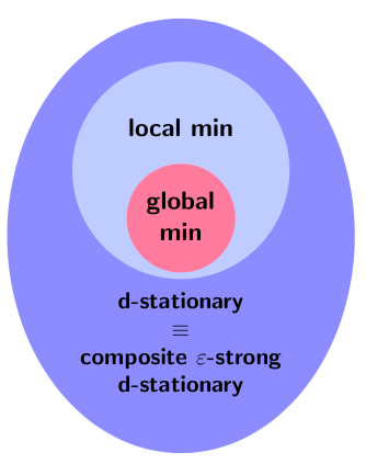
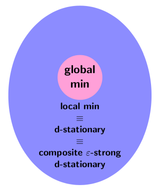
for sufficiently small $\varepsilon$
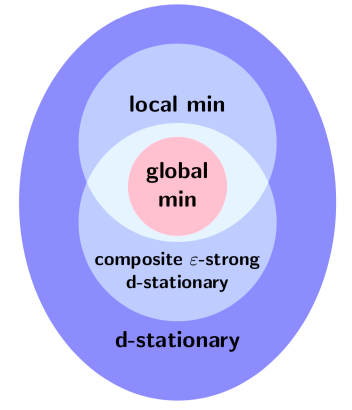
for large $\varepsilon$ for small $\varepsilon>0$ and affine $f_{j}(\,\bullet\,;\xi)$ and $g_{j}(\,\bullet\,;\xi)$

Figure 1: Diagram of the relationship between global/local minimizers and (composite $\varepsilon$-strong) d-stationary points.

To close this section, we point out that the computation of a d-stationary point of a difference-max optimization problem can be accomplished by an enhancement [39] of the original difference-of-convex algorithm (DCA) [29] that makes use of an arbitrary $\varepsilon>0$. The subsequent reference [33] shows that the so-computed d-stationary solution is actually $\varepsilon$-strong d-stationary. The more recent reference [10] further extends these references to a composite difference-max problem of which (10) is a special case. Thus the analysis in the next section about a d-stationary solution of (10) is computationally meaningful. This is in contrast to the analysis of minimizers of the problems (10) and (11) that is in general detached from computational tractability.

5 Consistency of D-stationary Solutions

We establish in this section the convergence as $N$ tends to infinity of composite $\varepsilon$-strong d-stationary solutions of (10) to a d-stationary solution of the population problem (11). Adding to the uniform Lipschitz continuity (13) of the functions $\left\{f_{j}\right\}_{j=1}^{k_{f}}$ and $\left\{g_{j}\right\}_{j=1}^{k_{g}}$, we impose the following assumptions.

Assumption 5.1.

(a1) Both $\mbox{Lip}_{f}(\xi)$ and $\mbox{Lip}_{g}(\xi)$ in the inequalities (13) are square integrable and $c_{0}>0$ exists such that for all $\xi$ in the probability-one subset $\Xi^{\,1}$ of $\Xi$, $\max\left(\,\mbox{Lip}_{f}(\xi),\,\mbox{Lip}_{g}(\xi)\,\right)\leq c_{0}$.

(a2) There exist square integrable functions $\mbox{Lip}_{\nabla f}(\xi)$ and $\mbox{Lip}_{\nabla g}(\xi)$ and a probability-one subset $\Xi^{\,1}_{\nabla}$ of $\Xi$ such that for $\xi\in\Xi^{\,1}_{\nabla}$ and for any $x$ and $y$ in $X$,

$$\left\{\begin{array}[]{ll}\left\|\,\nabla_{x}f_{j}(x;\xi)-\nabla_{x}f_{j}(y;\xi)\,\right\|_{2}\,\leq\,\mbox{Lip}_{\nabla f}(\xi)\,\left\|\,x-y\,\right\|_{2},\quad\forall\;j=1,\ldots,k_{f},\\[10.84006pt] \left\|\,\nabla_{x}g_{j}(x;\xi)-\nabla_{x}g_{j}(y;\xi)\,\right\|_{2}\,\leq\,\mbox{Lip}_{\nabla g}(\xi)\,\left\|\,x-y\,\right\|_{2},\quad\forall\;j=1,\ldots,k_{g}.\end{array}\right.$$

(a3) There exist square integrable functions $C_{f}(\xi)$ and $C_{g}(\xi)$ and a probability-one subset $\Xi^{\,2}_{\nabla}$ of $\Xi$ such that for all $\xi\in\Xi^{\,2}_{\nabla}$,

$$\left\{\begin{array}[]{ll}\displaystyle{\sup_{x\in X}}\,\left\|\,\nabla_{x}f_{j}(x;\xi)\,\right\|_{2}\,\leq\,C_{f}(\xi),\quad\forall\;j=1,\ldots,k_{f},\\[10.84006pt] \displaystyle{\sup_{x\in X}}\,\left\|\,\nabla_{x}g_{j}(x;\xi)\,\right\|_{2}\,\leq\,C_{g}(\xi),\quad\forall\;j=1,\ldots,k_{g}.\end{array}\right.$$

(b) There exist a square integrable function $\mbox{Lip}_{h}({\mbox{\boldmath$z$}})$ and a probability-one subset $\widehat{\cal Z}$ of ${\cal Z}$ such that for all ${\mbox{\boldmath$z$}}\in\widehat{\cal Z}$ and for any $t_{1}$ and $t_{2}\in\mathbb{R}$,

$$\left|\,h(t_{1};{\mbox{\boldmath$z$}})-h(t_{2};{\mbox{\boldmath$z$}})\,\right|\,\leq\,\mbox{Lip}_{h}({\mbox{\boldmath$z$}})\left|\,t_{1}-t_{2}\,\right|.$$

We let $\widehat{\Xi}\,\triangleq\,\Xi^{\,1}\,\cap\,\Xi^{\,1}_{\nabla}\,\cap\,\Xi^{\,2}_{\nabla}$ and $\widehat{\Omega}\,\triangleq\,\widehat{\Xi}\times\widehat{\cal Z}$. Note that ${\rm I}\!{\rm P}(\widehat{\Omega})=1$.

Notice that Assumptions (a2) and (a3) in 5.1 imply that

$${\rm I\!E}_{\widetilde{\omega}}\left[\,\displaystyle{\sup_{x\in X}}\,\left|\,h^{\updownarrow}\circ(\,m(x;\widetilde{\xi});\widetilde{{\mbox{\boldmath$z$}}}\,)\,\right|\,\right]\,<\,+\infty.$$

We begin with several lemmas that are essential to the proof of our main result. The first one is the classical uniform law of large numbers and its implication on the continuous convergence of random functions.

Lemma 5.2.

(c.f. [56, Lemma 3.10]) Let the bivariate function $\mathcal{L}:\mathbb{R}^{p}\times\Omega\to\mathbb{R}$ be such that ${\cal L}(\bullet,\omega)$ is continuous on $\mathbb{R}^{p}$ for almost all $\omega\in\Omega$. Let $X\subseteq\mathbb{R}^{p}$ be a compact set. Suppose that ${\rm I\!E}_{\widetilde{\omega}}\left[\,\displaystyle\sup_{x\in X}\,|\,\mathcal{L}(x;\widetilde{\omega})\,|\,\right]<+\infty$. Then

$$\lim_{N\rightarrow\infty}\,\sup_{x\in X}\,\left|\,\frac{1}{N}\sum_{n=1}^{N}\mathcal{L}(x;\omega^{\,n})-{\rm I\!E}_{\omega}\left[\,\mathcal{L}(x;\omega)\,\right]\,\right|\rightarrow 0\quad\mbox{almost surely}\,.$$

Moreover, if ${\rm I\!E}_{\widetilde{\omega}}\,{\cal L}(\bullet,\widetilde{\omega})$ is continuous on an open set containing $X$, then for any $x\in X$ and any sequence $\left\{x^{N}\right\}\subset X$ converging to $x$, it holds that

$$\lim_{N\rightarrow\infty}\,\left|\,\frac{1}{N}\sum_{n=1}^{N}\mathcal{L}\left(x^{N};\omega^{\,n}\right)-{\rm I\!E}_{\widetilde{\omega}}\,[\,\mathcal{L}(x;\widetilde{\omega})\,]\,\right|=0\hskip 12.0pt\mbox{almost surely}\,.$$

Lemma 5.3.

Suppose that Assumption 5.1 holds. Let $X\subseteq\mathbb{R}^{\,p}$ be a compact set. Then for any $\bar{x}\in\mathbb{R}^{\,p}$ and any $\varepsilon>0$,

$${\lim_{N\to+\infty}}\,\max\left(\,\begin{array}[]{l}\displaystyle{\sup_{x,y\in X}}\,\displaystyle{}\,\left|\,R^{\,\uparrow}_{N;\bar{x};\varepsilon}(x,y)-R^{\,\uparrow}_{\bar{x};\varepsilon}(x,y)\,\right|,\\[10.84006pt] \displaystyle{\sup_{x,y\in X}}\,\displaystyle{}\,\left|\,R^{\,\downarrow}_{N;\bar{x};\varepsilon^{\prime}}(x,y)-R^{\,\downarrow}_{\bar{x};\varepsilon}(x,y)\,\right|\end{array}\,\right)\,=\,0,\hskip 12.0pt\mbox{almost surely}.$$ (23)

Proof.

To prove this lemma, it suffices to check that

$$\left\{\begin{array}[]{ll}{\rm I\!E}_{\widetilde{\omega}}\left[\,\displaystyle{\sup_{x,y\in X}}\,h^{\uparrow}\left(\,f(y;\widetilde{\xi})-\displaystyle{\max_{j\in{\cal A}_{g;\varepsilon}(\bar{x};\widetilde{\xi})}}\,\left[\,g_{j}(x;\widetilde{\xi})+(y-x)^{\top}\nabla_{x}g_{j}(x;\widetilde{\xi})\,\right];\widetilde{{\mbox{\boldmath$z$}}}\,\right)\,\right]<+\infty,\\[18.06749pt] {\rm I\!E}_{\widetilde{\omega}}\left[\,\displaystyle{\sup_{x,y\in X}}\,h^{\downarrow}\left(\,\displaystyle{\max_{j\in{\cal A}_{f;\varepsilon}(\bar{x};\widetilde{\xi})}}\,\left[\,f_{j}(x;\widetilde{\xi})+(y-x)^{\top}\nabla_{x}f_{j}(x;\widetilde{\xi})\,\right]-g(y;\widetilde{\xi});\widetilde{{\mbox{\boldmath$z$}}}\,\right)\right]\,<\,+\infty\end{array}\right.$$ (24)

and then apply Lemma 5.2. By Assumption 5.1 (a2) and (a3), we have that for all pairs $(\xi,{\mbox{\boldmath$z$}})\in\widehat{\Omega}$,

$$\begin{array}[]{l}h^{\uparrow}\left(\,f(y;\xi)-\displaystyle\max_{j\in{\cal A}_{g;\varepsilon}(\bar{x};\,\xi)}\left[\,g_{j}(x;\xi)+(y-x)^{\top}\nabla_{x}g_{j}(x;\xi)\,\right];\,{\mbox{\boldmath$z$}}\,\right)\\[14.45377pt] \leq\,h^{\uparrow}\left(\,f(\bar{x};\xi)+\,\mbox{Lip}_{f}(\xi)\,\|\,y-\bar{x}\,\|_{2}-\,\displaystyle{\max_{j\in{\cal A}_{g;\varepsilon}(\bar{x};\,\xi)}}\,g_{j}(y;\xi)+\frac{\mbox{Lip}_{\nabla g}(\xi)\|\,y-x\,\|_{2}^{2}}{2};\,{\mbox{\boldmath$z$}}\,\right)\\[14.45377pt] \leq\,h^{\uparrow}\left(\,f(\bar{x};\xi)+\,\mbox{Lip}_{f}(\xi)\,\|\,y-\bar{x}\,\|_{2}-\,\displaystyle{\max_{j\in{\cal A}_{g;\varepsilon}(\bar{x};\,\xi)}}\,g_{j}(\bar{x};\xi)+\mbox{Lip}_{g}(\xi)\|\,y-\bar{x}\,\|_{2}+\frac{\mbox{Lip}_{\nabla g}(\xi)\|\,y-x\,\|_{2}^{2}}{2};\,{\mbox{\boldmath$z$}}\,\right)\\[14.45377pt] \leq\,h^{\uparrow}\left(\,f(\bar{x};\xi)-g(\bar{x};\xi);{\mbox{\boldmath$z$}}\,\right)+\,\mbox{Lip}_{h}({\mbox{\boldmath$z$}})\,\left[\,\mbox{Lip}_{f}(\xi)\,\|\,y-\bar{x}\,\|_{2}+\mbox{Lip}_{g}(\xi)\|\,y-\bar{x}\,\|_{2}+\displaystyle\frac{\mbox{Lip}_{\nabla g}(\xi)\|y-x\|_{2}^{2}}{2}\,\right]\\[14.45377pt] =\,h^{\uparrow}\left(\,m(\bar{x};\xi);{\mbox{\boldmath$z$}}\,\right)+\,\,\mbox{Lip}_{h}({\mbox{\boldmath$z$}})\,\left[\,\mbox{Lip}_{f}(\xi)\,\|\,y-\bar{x}\,\|_{2}+\mbox{Lip}_{g}(\xi)\|\,y-\bar{x}\,\|_{2}+\displaystyle\frac{\mbox{Lip}_{\nabla g}(\xi)\|\,y-x\,\|_{2}^{2}}{2}\,\right].\end{array}$$

By Assumption 5.1 (b) and setting $B=\text{Diam}(X)$, we further obtain that

$$\begin{array}[]{l}{\rm I\!E}_{\widetilde{\omega}}\left[\,\displaystyle\sup_{x,y\in X}h^{\uparrow}\left(\,f(y;\widetilde{\xi})-\displaystyle{\max_{j\in{\cal A}_{g;\varepsilon}(\bar{x};\widetilde{\xi})}}\,\left[\,g_{j}(x;\widetilde{\xi})+(y-x)^{\top}\nabla_{x}g_{j}(x;\widetilde{\xi})\,\right];\,\widetilde{{\mbox{\boldmath$z$}}}\,\right)\,\right]\\[14.45377pt] \leq\,{\rm I\!E}_{\widetilde{\omega}}\left[\,\displaystyle\sup_{x\in X}h^{\uparrow}\left(\,m(\bar{x};\widetilde{\xi});\widetilde{{\mbox{\boldmath$z$}}}\,\right)\,\right]+B\,{\rm I\!E}_{\widetilde{\omega}}\left[\,\mbox{Lip}_{h}(\widetilde{{\mbox{\boldmath$z$}}})\,\left(\mbox{Lip}_{f}(\widetilde{\xi})\,+\mbox{Lip}_{g}(\widetilde{\xi})\,+\displaystyle{\frac{B\,\mbox{Lip}_{\nabla g}(\widetilde{\xi})}{2}}\,\right)\,\right]\\[14.45377pt] <\,+\infty.\end{array}$$

This string of inequalities is enough to yield the first inequality in (24). The second inequality in (24) can be derived based on similar arguments and we omit the details here. ∎

From this point on, we will be working with infinite sequences $\{\omega^{n}\}_{n=1}^{\infty}$ of random realizations of the random variable pairs $(\widetilde{\xi},\widetilde{{\mbox{\boldmath$z$}}})$. For this purpose, we let $\Omega^{\infty}$ denote the $\infty$-fold Cartesian product of the sample space $\Omega$. Let $\mathcal{F}^{\infty}$ denote the sigma-algebra generated by subsets of $\Omega^{\infty}$, and let ${\rm I}\!{\rm P}_{\infty}$ be the corresponding probability measure defined on this sigma-algebra. Let ${\rm I\!E}_{\infty}$ be the expectation operator induced by ${\rm I}\!{\rm P}_{\infty}$. Throughout the analysis, we fix the probability tuple $\left(\Omega^{\infty},{\cal F}^{\infty},{\rm I}\!{\rm P}_{\infty},{\rm I\!E}_{\infty}\right)$. We say that an event $E\in{\cal F}^{\infty}$ happens “almost surely” if ${\rm I}\!{\rm P}_{\infty}(E)=1$. Without loss of generality, we assume that the probability-one set $\widehat{\Omega}\triangleq\widehat{\Xi}\times{\cal Z}^{\,1}$ is such that the limit (23) in Lemma 5.3 holds for all families $\{\omega^{n}\}_{n=1}^{\infty}\subset\widehat{\Omega}^{\,\infty}$. In the rest of the paper, for any such family of random realizations, we let, for each $N$, $x^{N;\varepsilon}(\omega^{N})$ be a composite $\varepsilon$-strong d-stationary point of (10) corresponding to a given scalar $\varepsilon\geq 0$. (The case $\varepsilon=0$ refers to a d-stationary point.) We will write $x^{N}$ for $x^{N;\varepsilon}(\omega^{N})$ if the context is clear.

The following lemma is the key step to establish our main result of this section.

Lemma 5.4.

Suppose that Assumption 5.1 holds. Let $\varepsilon>0$ be given and let $\{\omega^{n}\}_{n=1}^{\infty}\subset\widehat{\Omega}$ be arbitrary. If the sequence $\{x^{N;\varepsilon}(\omega^{N})\}$ converges to $x^{\infty}$, then $x^{\infty}$ solves the nonconvex optimization problem

$$\operatornamewithlimits{minimize}_{x\in X}\;R_{x^{\infty};\varepsilon^{\prime}}(x,x^{\infty})$$

for every $\varepsilon^{\,\prime}\in[0,\varepsilon)$. In particular, $x^{\infty}$ is also a minimizer of $R_{x^{\infty}}(\bullet,x^{\infty})$ on $X$.

Proof.

Write $x^{N}\equiv x^{N;\varepsilon}(\omega^{N})$ for simplicity. Since $x^{N}$ converges to $x^{\infty}$, then for sufficiently large $N$, the following inclusions hold for all $\varepsilon^{\,\prime}\in[0,\varepsilon)$ and all $\xi\in\widehat{\Xi}$,

$${\cal A}_{f;\varepsilon^{\,\prime}}(x^{\infty};\xi)\,\subseteq\,{\cal A}_{f;\varepsilon}(x^{N};\xi)\hskip 12.0pt\mbox{and}\hskip 12.0pt{\cal A}_{g;\varepsilon^{\,\prime}}(x^{\infty};\xi)\,\subseteq\,{\cal A}_{g;\varepsilon}(x^{N};\xi),$$

by Lemma 4.1. Furthermore, since $x^{N}$ is a composite $\varepsilon$-strong d-stationary point of (10), it follows from (21) that for any $x\in X$,

$$\begin{array}[]{l}{\cal M}_{N}(x^{N})\,\leq\,\displaystyle\frac{1}{N}\sum_{n=1}^{N}h^{\uparrow}\left(f(x;\xi^{\,n})-\displaystyle{\max_{j\in{\cal A}_{g;\varepsilon}(x^{N};\,\xi^{\,n})}}\,\left[\,g_{j}(x^{N};\xi^{\,n})+\nabla_{x}g_{j}\left(x^{N};\xi^{\,n}\right)^{\top}(x-x^{N})\,\right];{\mbox{\boldmath$z$}}^{\,n}\right)\\[18.06749pt] \hskip 50.58878pt+\displaystyle{\frac{1}{N}}\,\displaystyle{\sum_{n=1}^{N}}\,h^{\downarrow}\left(\displaystyle{\max_{j\in{\cal A}_{f;\varepsilon}(x^{N};\,\xi^{\,n})}}\,\left[\,f_{j}(x^{N};\xi^{\,n})+\nabla_{x}f_{j}\left(x^{N};\xi^{\,n}\right)^{\top}(x-x^{N})\,\right]-g(x;\xi^{\,n});{\mbox{\boldmath$z$}}^{\,n}\right)\\[18.06749pt] \leq\,R_{N;x^{\infty};\varepsilon^{\prime}}(x;x^{N})\\[10.84006pt] =\,\left[\,R_{N;x^{\infty};\varepsilon^{\prime}}(x,x^{N})-R_{x^{\infty};\varepsilon^{\prime}}(x,x^{N})\,\right]+\left[\,R_{x^{\infty};\varepsilon^{\prime}}(x,x^{N})-R_{x^{\infty};\varepsilon^{\prime}}(x,x^{\infty})\,\right]+R_{x^{\infty};\varepsilon^{\prime}}(x,x^{\infty})\\[10.84006pt] \leq\,\left[\,\displaystyle{\sup_{x^{\,\prime},y\,\in\,X}}\,\left|\,R_{N;x^{\infty};\varepsilon^{\prime}}(x^{\,\prime},y)-R_{x^{\infty};\varepsilon^{\prime}}(x^{\,\prime},y)\,\right|\,\right]+\left[\,\displaystyle{\sup_{x^{\,\prime}\in X}}\,\left|\,R_{x^{\infty};\varepsilon^{\prime}}(x^{\,\prime},x^{N})-R_{x^{\infty};\varepsilon^{\prime}}(x^{\,\prime},x^{\infty})\,\right|\,\right]\\[18.06749pt] \hskip 12.0pt\hskip 12.0pt+\,R_{x^{\infty};\varepsilon^{\prime}}(x,x^{\infty}).\end{array}$$

Observe that

$$\begin{array}[]{l}\displaystyle\sup_{x\in X}\left|\,R_{x^{\infty};\varepsilon^{\prime}}^{\uparrow}(x,x^{N})-R_{x^{\infty};\varepsilon^{\prime}}^{\uparrow}(x,x^{\infty})\,\right|\\[14.45377pt] \leq\,{\rm I\!E}_{\widetilde{\omega}}\left[\,\mbox{Lip}_{h}(\widetilde{{\mbox{\boldmath$z$}}})\left|\,g(x^{\infty};\widetilde{\xi})-g(x^{N};\widetilde{\xi})+\displaystyle{\max_{j\in{\cal A}_{g;\varepsilon^{\prime}}(x^{\infty};\widetilde{\xi})}}\,\left[\,\nabla_{x}g_{j}(x^{\infty};\widetilde{\xi})^{\top}\,x^{\infty}-\nabla_{x}g_{j}(x^{N};\widetilde{\xi})^{\top}\,x^{N}\,\right]\,\right|\,\right]\\[14.45377pt] \hskip 12.0pt+\,\displaystyle{\sup_{x\in X}}\,\left[\,{\rm I\!E}_{\widetilde{\omega}}\,\mbox{Lip}_{h}(\widetilde{{\mbox{\boldmath$z$}}})\,\|\,x\,\|_{2}\,\max_{j\in{\cal A}_{g;\varepsilon^{\prime}}(x^{\infty};\widetilde{\xi})}\,\left\|\,\nabla_{x}g_{j}(x^{N};\widetilde{\xi})-\nabla_{x}g_{j}(x^{\infty};\widetilde{\xi})\,\right\|_{2}\right]\\[14.45377pt] \leq\,{\rm I\!E}_{\widetilde{\omega}}\left[\mbox{Lip}_{h}(\widetilde{{\mbox{\boldmath$z$}}})\left|\,g(x^{\infty};\widetilde{\xi})-g(x^{N};\widetilde{\xi})+\displaystyle{\max_{j\in{\cal A}_{g;\varepsilon^{\prime}}(x^{\infty};\,\xi)}}\,\left[\,\nabla_{x}g_{j}(x^{\infty};\widetilde{\xi})^{\top}\,x^{\infty}-\nabla_{x}g_{j}(x^{N};\widetilde{\xi})^{\top}\,x^{N}\,\right]\,\right|\,\right]\\[14.45377pt] \hskip 12.0pt+\,\text{Diam}(X)\,\left[\,{\rm I\!E}_{\widetilde{\omega}}\,\mbox{Lip}_{h}(\widetilde{{\mbox{\boldmath$z$}}})\,\displaystyle{\max_{j\in{\cal A}_{g;\varepsilon^{\prime}}(x^{\infty};\,\xi)}}\,\left\|\,\nabla_{x}g_{j}(x^{N};\widetilde{\xi})-\nabla_{x}g_{j}(x^{\infty};\widetilde{\xi})\,\right\|_{2}\right].\end{array}$$

By the dominating convergence theorem and the continuity of both $g(\bullet;\xi)$ and $\nabla_{x}g_{j}(\bullet;\xi)$ from Assumption 5.1, it follows that the last sum goes to $0$ as $N\to\infty$. Similarly, we can derive $\displaystyle\lim_{N\to\infty}\sup_{x\in X}\left|\,R_{x^{\infty};\varepsilon^{\prime}}^{\downarrow}(x,x^{N})-R_{x^{\infty};\varepsilon^{\prime}}^{\downarrow}(x,x^{\infty})\,\right|=0$. It then follows from Lemma 5.3 that for all $x\in X$,

$$R_{x^{\infty};\varepsilon^{\prime}}(x^{\infty},x^{\infty})\,=\ {\cal M}(x^{\infty})\,=\,\lim_{N\rightarrow\infty}{\cal M}_{N}(x^{N})\,\leq\,R_{x^{\infty};\varepsilon^{\prime}}(x,x^{\infty}),$$

which is the first conclusion of this lemma. The second conclusion can be obtained by noting that $R_{x^{\infty};\varepsilon^{\prime}}(x,x^{\infty})\leq R_{x^{\infty}}(x,x^{\infty})$ ∎

Lemma 5.5.

Suppose that Assumption 5.1 holds. Then for all $\omega\in\widehat{\Omega}$, any $\varepsilon>0$, and all $\bar{x}\in X$,

$$\left\{\begin{array}[]{ll}\left|\,r^{\uparrow}_{\bar{x};\varepsilon}(x,\bar{x};\omega)-r_{\bar{x};\varepsilon}^{\uparrow}(y,\bar{x};\omega)\,\right|\,\leq\,\mbox{Lip}_{h}({\mbox{\boldmath$z$}})\left[\,\text{Lip}_{f}(\xi)+C_{g}(\xi)\,\right]\,\|\,x-y\,\|_{2}\\[7.22743pt] \left|\,r^{\downarrow}_{\bar{x};\varepsilon}(x,\bar{x};\omega)-r_{\bar{x};\varepsilon}^{\uparrow}(y,\bar{x};\omega)\,\right|\,\leq\,\mbox{Lip}_{h}({\mbox{\boldmath$z$}})\left[\,C_{f}(\xi)+\text{Lip}_{g}(\xi)\,\right]\,\|\,x-y\,\|_{2}\end{array}\right.,\quad\forall\;x,y\,\in\,\mathbb{R}^{p}.$$

Proof.

This can be easily seen by the following string of inequalities

$$\begin{array}[]{rl}&\left|\,r^{\uparrow}_{\bar{x};\varepsilon}(x,\bar{x};\omega)-r^{\uparrow}_{\bar{x};\varepsilon}(y,\bar{x};\omega)\,\right|\\[10.84006pt] \leq&\mbox{Lip}_{h}({\mbox{\boldmath$z$}})\left(\,\left|\,f(x;\xi)-f(y;\xi)\,\right|+\displaystyle\max_{j\in{\cal A}_{g;\varepsilon}(\bar{x};\xi)}\left|\,(x-y)^{\top}\nabla_{x}g_{j}(\bar{x};\xi)\,\right|\,\right)\\[14.45377pt] \leq&\mbox{Lip}_{h}({\mbox{\boldmath$z$}})\left[\,\text{Lip}_{f}(\xi)+C_{g}(\xi)\,\right]\,\|\,x-\,y\|_{2}\end{array}$$

and similar ones for $r^{\downarrow}_{\bar{x};\varepsilon}(\bullet,\bar{x};\omega)$. ∎

Let $\mathcal{D}$ denote the set of directional stationary solution of (11), i.e.,

$$\mathcal{D}\,\triangleq\,\left\{\,\bar{x}\in X\,\mid\mathcal{M}^{\,\prime}(\bar{x};x-\bar{x})\geq 0,\hskip 12.0pt\forall\;x\in X\,\right\}.$$

For any $x^{\,\prime}\in\mathbb{R}^{n}$, we also let $\mbox{dist}(x^{\,\prime},\mathcal{D})\triangleq\displaystyle{\inf_{x\in{\cal D}}}\,\|\,x-x^{\,\prime}\|$, where $\|\bullet\|$ denotes the Euclidean norm of vectors. We are now ready to present the main convergence result, which shows that the limit of the empirical composite $\varepsilon$-strong d-stationary points is a d-stationary point of the population risk under mild conditions.

Theorem 5.6.

Suppose that Assumption 5.1 holds. Let $\varepsilon>0$ be given. Thus

$${\rm I}\!{\rm P}_{\infty}\left(\{\omega^{n}\}_{n=1}^{\infty}\subset\widehat{\Omega}\,\left|\,\displaystyle{\lim_{N\to\infty}}\,\mbox{dist}(x^{N;\varepsilon}(\omega^{N}),\mathcal{D})\,=\,0\,\right.\right)\,=\,1.$$ (25)

In particular, if $\{x^{N;\varepsilon}(\omega^{N})\}$ converges to $x^{\infty}$ almost surely, then $x^{\infty}\in{\cal D}$.

Proof.

Suppose that (25) fails to hold. Then there exists an event set $\mathcal{E}$ with positive probability such that for any family $\{\omega^{n}\}_{n=1}^{\infty}$ in $\mathcal{E}$, we have $\displaystyle{\liminf_{N\to\infty}}\mbox{dist}(x^{N;\varepsilon}(\omega^{N}),\mathcal{D})\,>\,0$. Let $\{\omega^{n}\}_{n=1}^{\infty}$ be any such family. Since $X$ is compact, by passing to a subsequence if necessary, we may assume without loss of generality that the entire sequence $\left\{x^{N;\varepsilon}(\omega^{N})\right\}$ converges to a point $x^{\infty}$. By Lemma 5.4, we may deduce that $x^{\infty}$ is an optimal solution of $\displaystyle\operatornamewithlimits{minimize}_{y\in X}\;R_{x^{\infty}}(y,x^{\infty})$. Hence, we have that for any $x\in X$,

$$\begin{array}[]{ll}\left(R_{x^{\infty}}^{\,\uparrow}(\,\bullet\,,x^{\infty})\right)^{\prime}(x^{\infty};x-x^{\infty})+\left(R_{x^{\infty}}^{\,\downarrow}(\,\bullet\,,x^{\infty})\right)^{\prime}(x^{\infty};x-x^{\infty})\\[10.84006pt] =\,{\rm I\!E}_{\omega}\left[(h^{\uparrow})^{\prime}(\,\bullet\,;{\mbox{\boldmath$z$}})\left(m(x^{\infty};\xi);\,f(\bullet;\xi)^{\prime}(x^{\infty};x-x^{\infty})-\displaystyle\max_{j\in{\cal A}_{g}(x^{\infty};\,\xi)}\nabla_{x}g_{j}(x^{\infty};\xi)^{\top}(x-x^{\infty})\,\right)\right]\\[14.45377pt] +\,{\rm I\!E}_{\omega}\left[(h^{\downarrow})^{\prime}(\,\bullet\,;{\mbox{\boldmath$z$}})\left(m(x^{\infty};\xi);\,\displaystyle\max_{j\in{\cal A}_{f}(x^{\infty};\xi)}\nabla_{x}f_{j}(x^{\infty},\xi)^{\top}(x-x^{\infty})-g(\bullet;\xi)^{\prime}(x^{\infty};x-x^{\infty})\,\right)\,\right]\\[14.45377pt] =\,\mathcal{M}^{\prime}(x^{\infty};x-x^{\infty})\geq 0,\end{array}$$

where the equality is obtained by exchanging the directional derivative and the expectation based on [52, Theorem 7.44] and Lemma 5.5. ∎

Combining Theorem 5.6 with Proposition 4.7, we obtain sufficient conditions for the consistency of the d-stationary points. Before stating this result, we note that the $\bar{\varepsilon}$ in the latter proposition depends on the sample set $\{\xi^{\,n}\}_{n=1}^{N}$. In what follows, we provide a sufficient condition that guarantees the existence of a uniform $\bar{\varepsilon}$ that is independent of the samples so that the proposition can be applied to the sampled d-stationary points. This condition is a sort of “sufficient separation” between the component functions in the two pointwise maximum functions $f(\bullet;\xi)$ and $g(\bullet;\xi)$ at a given point $\bar{x}$. Specifically, we say that the (pointwise) sufficient separation condition holds at $\bar{x}\in X$ if there exist positive constants $\delta$ and $c$ and a probability-one set $\Xi^{\,ss}_{\bar{x}}$ such that for all $\xi\in\Xi^{\,ss}_{\bar{x}}$,

$$\begin{array}[]{rll}\displaystyle{\inf_{x\in\mathbb{B}_{\delta}(\bar{x})}}\,\left[\,\displaystyle{\max_{j\in{\cal A}_{f}(x;\xi)}}\,f_{j}(x;\xi)-\displaystyle{\max_{j\notin{\cal A}_{f}(x;\xi)}}\,f_{j}(x;\xi)\,\right]&\geq&c\\[14.45377pt] \displaystyle{\inf_{x\in\mathbb{B}_{\delta}(\bar{x})}}\,\left[\,\displaystyle{\max_{j\in{\cal A}_{g}(x;\xi)}}\,g_{j}(x;\xi)-\displaystyle{\max_{j\notin{\cal A}_{g}(x;\xi)}}\,g_{j}(x;\xi)\,\right]&\geq&c.\end{array}$$

We first establish a lemma that establishes the equality of various index sets for points near any given point $\bar{x}$ satisfying this condition.

Lemma 5.7.

Suppose that Assumption 5.1 holds. If $\bar{x}$ satisfies the sufficient separation condition with the associated probability-one set $\Xi^{\,ss}_{\bar{x}}$, then there exist positive constants $\bar{\varepsilon}$ and $\bar{x}$ such that $\mathcal{A}_{f;\varepsilon}(x;\xi)=\mathcal{A}_{f}(\bar{x};\xi)$ and $\mathcal{A}_{g;\varepsilon}(x;\xi)=\mathcal{A}_{g}(\bar{x};\xi)$ for all $\varepsilon\in[\,0,\bar{\varepsilon}\,]$, all $x\in\mathbb{B}_{\bar{\delta}}(\bar{x})$, and all $\xi\in\widehat{\Xi}\,\cap\,\Xi^{\,ss}_{\bar{x}}$.

Proof.

To simplify the notation somewhat, we assume in the proof below that the two probability-one sets $\widehat{\Xi}$ and $\Xi^{\,ss}_{\bar{x}}$ coincide. Let scalars $\bar{\varepsilon}\in(\,0,\,c/2\,]$ and $\bar{\delta}\in\left(\,0,\min\left(\,\delta,\,\displaystyle{\frac{\bar{\varepsilon}}{4c_{0}}}\,\right)\,\right)$ be arbitrary. By Lemma 4.1, for all $\varepsilon^{\,\prime}\in[0,\bar{\varepsilon}/2]$, all $\xi\in\widehat{\Xi}$, and all pairs $x^{1}$ and $x^{2}$ in $X$ satisfying $\|\,x^{1}-x^{2}\,\|_{2}\leq\bar{\delta}$, we have ${\cal A}_{f;\varepsilon^{\,\prime}}(x^{1};\xi)\subseteq{\cal A}_{f;\bar{\varepsilon}}(x^{2};\xi)$ and ${\cal A}_{g;\varepsilon^{\,\prime}}(x^{1};\xi)\subseteq{\cal A}_{g;\bar{\varepsilon}}(x^{2};\xi)$. In particular, with $\varepsilon^{\,\prime}=0$, we have $\mathcal{A}_{f}(\bar{x};\xi)\subseteq\mathcal{A}_{f;\bar{\varepsilon}}(x;\xi)$ and $\mathcal{A}_{g}(\bar{x};\xi)\subseteq\mathcal{A}_{g;\bar{\varepsilon}}(x;\xi)$ for all $x\in\mathbb{B}_{\bar{\delta}}(\bar{x})$ and all $\xi\in\widehat{\Xi}$. We claim that the reverse inclusions hold. Indeed, we derive from the proof of Proposition 4.7 that $\mathcal{A}_{f;\varepsilon}(x;\xi)=\mathcal{A}_{f}(x;\xi)$ and $\mathcal{A}_{g;\varepsilon}(x;\xi)=\mathcal{A}_{g}(x;\xi)$ for all $\varepsilon\in[\,0,\,c/2\,]$, all $x\in\mathbb{B}_{\bar{\delta}}(\bar{x})$, and all $\xi\in\widehat{\Xi}$. Then for any $x\in\mathbb{B}_{\bar{\delta}}(\bar{x})$, if $j\in\mathcal{A}_{f;\bar{\varepsilon}}(x;\xi)$, we have $j\in\mathcal{A}_{f}(x;\xi)$; thus $f_{j}(x;\xi)\geq\displaystyle{\max_{1\leq i\leq k_{f}}}\,f_{i}(x;\xi)$. This implies that

$$c_{0}\,\|\bar{x}-x\|_{2}+f_{j}(\bar{x},\xi)\geq f_{j}(x,\xi) \geq\max_{1\leq i\leq k_{f}}f_{i}(\bar{x},\xi)+\max_{1\leq i\leq k_{f}}f_{i}(x,\xi)-\max_{1\leq i\leq k_{f}}f_{i}(\bar{x},\xi)$$

$$\geq\max_{1\leq i\leq k_{f}}f_{i}(\bar{x},\xi)-c_{0}\,\|\bar{x}-x\|_{2},$$

which further yields

$$f_{j}(\bar{x},\xi)\geq\max_{1\leq i\leq k_{f}}f_{i}(\bar{x},\xi)-2c_{0}\,\|\bar{x}-x\|_{2}.$$

We thus obtain $j\in\mathcal{A}_{f;\bar{\varepsilon}}(\bar{x};\xi)=\mathcal{A}_{f}(\bar{x};\xi)$. Therefore, ${\cal A}_{f;\bar{\varepsilon}}(x;\xi)=\mathcal{A}_{f}(\bar{x};\xi)={\cal A}_{f;\varepsilon^{\,\prime}}(\bar{x};\xi)$ for all $\varepsilon^{\,\prime}\in[\,0,\bar{\varepsilon}\,]$, all $x\in\mathbb{B}_{\bar{\delta}}(\bar{x})$ and all $\xi\in\widehat{\Xi}$. Similarly we can prove the corresponding conclusion for $g$. ∎

Relying on Lemma 5.7, we have the following corollary of Theorem 5.6 about the d-stationarity of convergent sequence of d-stationarity points of the empirical problems.

Corollary 5.8.

Suppose that Assumptions 5.1 holds. Let $\{\omega^{n}\}_{n=1}^{\infty}\subset\widehat{\Omega}$ be arbitrary. For each positive integer $N$, let $x^{N}(\omega^{N})$ be a d-stationary point of (10) corresponding to $\{\omega^{n}\}_{n=1}^{N}$. If the sequence $\{x^{N}(\omega^{N})\}$ converges to $x^{\infty}$ satisfying the sufficient separation condition, then $x^{\infty}\in{\cal D}$.

Proof.

By Lemma 5.7, it follows that for some scalar $\bar{\varepsilon}>0$, it holds that for all $N$ sufficiently large, $\mathcal{A}_{f;\bar{\varepsilon}}(x^{N}(\omega^{N});\xi^{n})=\mathcal{A}_{f}(x^{N}(\omega^{N});\xi^{n})$ and $\mathcal{A}_{g;\bar{\varepsilon}}(x^{N}(\omega^{N});\xi^{n})=\mathcal{A}_{g}(x^{N}(\omega^{N});\xi^{n})$. Therefore, $x^{N}(\omega^{N})$ is a composite $\bar{\varepsilon}$-strong d-stationary point of (10) for all $N$ sufficiently large. The desired conclusion follows readily from Theorem 5.6. ∎

Remark 5.9.

It is possible to state a probabilistic conclusion of Corollary 5.8 similar to that in Theorem 5.6. For this to hold, we need to strengthen the sufficient separation condition to all d-stationary solutions in ${\cal D}$; more importantly, the same constants $c$ and $\delta$ have to hold uniformly for all such solutions. We omit the details and leave the Corollary in its pointwise form as stated above.

6 Asymptotic Distribution of the Stationary Values

In this and and the next section, we will work with sequences of composite $\varepsilon$-strong d-stationary solution of (10) for an arbitrary fixed $\varepsilon>0$. Our goal in this section is to derive an asymptotic distribution of the sequence of stationary values $\{{\cal M}_{N}(x^{N})\}$, where for each $N$, $x^{N}$ is a composite $\varepsilon$-strong d-stationary solution of (10), under the following piecewise affine assumption:

Assumption 6.1.

The function $m(\bullet;\xi)$ is a piecewise affine function, i.e., each $f_{j}(\bullet;\xi)$ and $g_{j}(\bullet\,;\xi)$ are affine functions.

An important consequence of this special structure is the following lemma.

Lemma 6.2.

Suppose that Assumption 5.1 (a1) and Assumption 6.1 hold. Then for any $\varepsilon>0$, there exists $\delta>0$ such that for any $\varepsilon^{\prime}\in\left[0,\frac{\varepsilon}{2}\right]$, any $x$ and $\bar{x}$ satisfying $\|x-\bar{x}\|_{2}\leq\delta$, and all $\omega\in\widehat{\Omega}$,

$$r^{\updownarrow}_{\bar{x};\varepsilon^{\prime}}(x,\bar{x};\omega)\,=\,r^{\updownarrow}_{x;\varepsilon}(x,x;\omega)\,=\,r^{\updownarrow}_{x}(x,x;\omega).$$ (26)

Hence, for any family $\{\omega^{n}\}_{n=1}^{\infty}\subset\widehat{\Omega}$

$$R_{N;\bar{x};\varepsilon^{\prime}}(x,\bar{x})\,=\,R_{N;x;\varepsilon}(x,x)\,=\,{\cal M}_{N}(x)\hskip 12.0pt\mbox{and}\hskip 12.0ptR_{\bar{x};\varepsilon^{\prime}}(x,\bar{x})=R_{x;\varepsilon}(x,x)\,=\,{\cal M}(x).$$

Proof.

It follows from Lemma 4.1 that there exists a positive scalar $\delta$ such that for any $\varepsilon^{\prime}\in[\,0,\frac{\varepsilon}{2}\,]$ and any $x$ and $\bar{x}$ satisfying $\|x-\bar{x}\|_{2}\leq\delta$, and any $\xi$ in the probability-one set $\widehat{\Xi}$,

$${\cal A}_{f}(x;\xi)\,\subseteq{\cal A}_{f;\varepsilon^{\prime}}(\bar{x};\xi)\,\subseteq\,{\cal A}_{f;\varepsilon}(x;\xi)\hskip 12.0pt\mbox{and}\hskip 12.0pt{\cal A}_{g}(x;\xi_{n})\subseteq{\cal A}_{g;\varepsilon^{\prime}}(\bar{x};\xi)\,\subseteq\,{\cal A}_{g;\varepsilon}(x;\xi)$$

Noticing that when $m(\bullet;\xi)$ is a piecewise affine function, we have $r^{\updownarrow}_{\bar{x};\varepsilon}(x,x^{1};\omega)=r^{\updownarrow}_{\bar{x};\varepsilon}(x,x^{2};\omega)$ for any $x$, $x^{1}$, $x^{2}$, and $\bar{x}$ in $X$, any $\varepsilon\geq 0$, and any $\omega\in\widehat{\Omega}$. Therefore, for any $\varepsilon^{\prime}\in\left[0,\frac{\varepsilon}{2}\right]$, and any $x$ and $\bar{x}$ satisfying $\|x-\bar{x}\|_{2}\leq\delta$, we derive for any $\omega\in\widehat{\Omega}$,

$$\begin{array}[]{lll}r^{\updownarrow}_{\bar{x};\varepsilon^{\prime}}(x,\bar{x};\omega)\,=\,r^{\updownarrow}_{\bar{x};\varepsilon^{\prime}}(x,x;\omega)&\leq&r^{\updownarrow}_{x}(x,x;\omega)\\[7.22743pt] &=&r^{\updownarrow}_{x;\varepsilon}(x,x;\omega)\,\leq\,r^{\updownarrow}_{\bar{x};\varepsilon^{\prime}}(x,x;\omega)\,=\,r^{\updownarrow}_{\bar{x};\varepsilon^{\prime}}(x,\bar{x};\omega).\end{array}$$

Consequently, equalities hold throughout, establishing the equalities in (26). ∎

An interesting consequence of Lemma 6.2 is that if $x^{\infty}$ is as described in Lemma 5.4, then $x^{\infty}$ is a local minimizer of the population level problem (11). This observation enables us to establish the following consistency result of local minima.

Corollary 6.3.

Suppose that Assumption 5.1 (a1) and Assumption 6.1 hold. If $\{x^{N;\varepsilon}(\omega^{N})\}$ converges to $x^{\infty}$ almost surely, then $x^{\infty}$ is a local minimizer of the population level problem (11).

Proof.

Under the given assumptions, we know if $\{x^{N;\varepsilon}(\omega^{N})\}$ converges to $x^{\infty}$ almost surely, then $x^{\infty}\in{\cal D}$. By Lemma 6.2, as long as $\|x-x^{\infty}\|_{2}\leq\delta$, we have $R_{x^{\infty};\varepsilon^{\prime}}(x,x^{\infty})=R_{x;\varepsilon}(x,x)={\cal M}(x)$. Since $x^{\infty}\in\displaystyle{\operatornamewithlimits{\mbox{argmin}}_{x\in X}}\,R_{x^{\infty};\varepsilon^{\prime}}(x,x^{\infty})$, we may conclude that $x^{\infty}$ minimizes ${\cal M}(x)$ locally on $X$. ∎

Besides being instrumental in establishing the consistency of a convergent sequence of composite $\varepsilon$-strong d-stationary solutions of (10), Lemma 5.4, along with Lemma 6.2, enables us to derive the following theorem that provides the asymptotic distribution of the stationary values ${\cal M}_{N}(x^{N})$ for such a sequence $\{x^{N}\}$. In what follows, we use the notation $\xrightarrow{d}$ to denote the convergence in distribution, and $\mathcal{N}(\mu,\sigma^{2})$ denotes the normal distribution with mean $\mu$ and variance $\sigma^{2}$. In addition, we use $\mbox{Var}[\bullet]$ to represent the variance of a random variable. We recall the objective function ${\cal L}(x;\omega)=h(m(x;\xi);{\mbox{\boldmath$z$}})$ of the population problem (11).

Theorem 6.4.

Suppose Assumptions 5.1 and 6.1 hold. Let $\{x^{N;\varepsilon}\}$ be a composite $\varepsilon$-strong d-stationary point of (10) corresponding to a family $\{\omega^{n}\}_{n=1}^{\infty}\subset\widehat{\Omega}$. If $x^{N;\varepsilon}$ converges to $x^{\infty}$ almost surely and ${\cal L}(x^{\infty};\bullet)$ is square integrable, then

$$\sqrt{N}\,\left[\,{\cal M}_{N}(x^{N;\varepsilon})-{\cal M}(x^{\,\infty})\,\right]\,\xrightarrow{d}\,\inf_{x\in S}\;\mathbb{G}_{x},$$

where $\mathbb{G}_{x}$ follows $\mathcal{N}\left(\,0,\mbox{Var}\left[{\cal L}(x;\widetilde{\omega})\right]\,\right)$ and $S\triangleq\displaystyle{\operatornamewithlimits{\mbox{argmin}}_{x\in\mathbb{B}_{\delta}(x^{\infty})}}\,{\cal M}(x)$ where $\delta$ is such that Lemma 6.2 holds. In particular, if $S=\{x^{\infty}\}$, then

$$\sqrt{N}\left({\cal M}_{N}(x^{N;\varepsilon})-{\cal M}(x^{\,\infty})\right)\,\xrightarrow{d}\,\mathcal{N}(0,\mbox{Var}\left[{\cal L}(x^{\infty};\widetilde{\omega})\right]).$$

Proof.

As $x^{N;\varepsilon}$ converges to $x^{\infty}$ almost surely, it follows from Lemma 6.2 that for all such sufficiently large $N$ and any $\varepsilon^{\prime}\in\left[\,0,\frac{\varepsilon}{2}\,\right]$,

$$\begin{array}[]{l}\sqrt{N}\,\left[\,{\cal M}_{N}(x^{N;\varepsilon})-{\cal M}(x^{\,\infty})\,\right]\,=\,\sqrt{N}\,\left[\,R_{N;x^{N;\varepsilon}}(x^{N;\varepsilon},x^{N;\varepsilon})-R_{x^{\,\infty};\varepsilon^{\prime}}(x^{\,\infty},x^{\,\infty})\,\right]\\[7.22743pt] =\,\sqrt{N}\,\left[\,R_{N;x^{\,\infty};\varepsilon^{\prime}}(x^{N},x^{\,\infty})-R_{x^{\,\infty};\varepsilon^{\prime}}(x^{\,\infty},x^{\,\infty})\,\right],\end{array}$$

almost surely. Notice that for any $\varepsilon^{\prime}\in\left[\,0,\frac{\varepsilon}{2}\,\right]$,

$$R_{N;x^{\,\infty};\varepsilon^{\prime}}(x^{N},x^{\,\infty})\,=\,R_{N;x^{N;\varepsilon};\varepsilon}(x^{N},x^{N})\leq R_{N;x^{N;\varepsilon};\varepsilon}(x,x^{N;\varepsilon})\,\leq\,R_{N;x^{\infty};\varepsilon^{\prime}}(x,x^{N}),\quad\forall\;x\in X,$$

almost surely. This implies that $x^{N;\varepsilon}\in\displaystyle\operatornamewithlimits{argmin}_{x\in X}\,R_{N;x^{\,\infty};\varepsilon^{\prime}}(x,x^{\,\infty})$ almost surely. We also know that $x^{\infty}\in\displaystyle\operatornamewithlimits{argmin}_{x\in X}\,R_{x^{\,\infty};\varepsilon^{\prime}}(x,x^{\,\infty})$. It follows from Lemma 5.5 that there exists a square integrable function $C(\omega)$ such that for all $\omega\in\widehat{\Omega}$,

$$\left|{r}_{x^{\infty};\varepsilon^{\prime}}(x^{1},x^{\infty};\omega)-{r}_{x^{\infty};\varepsilon^{\prime}}(x^{2},x^{\infty};\omega)\right|\,\leq\,C(\omega)\,\|\,x^{1}-x^{2}\,\|_{2},$$

which shows that [52, Condition (A2), page 164] holds. In addition, since ${r}_{x^{\infty};\varepsilon^{\prime}}(x^{\infty},x^{\infty};\widetilde{\omega})={\cal L}(x^{\infty};\widetilde{\omega})$ is square integrable, [52, Condition (A1), page 164] is satisfied. By applying [52, Theorem 5.7] and restricting to the almost sure set, we can derive that

$$\sqrt{N}\,\left[\,{\cal M}_{N}(x^{N})-{\cal M}(x^{\,\infty})\,\right]\,\xrightarrow{d}\,\inf_{x\in{\cal S}}\;\mathbb{G}_{x},$$

where $\mathbb{G}_{x}$ follows $\mathcal{N}\left(\,0,\mbox{Var}\left[{r}_{x^{\infty};\varepsilon^{\prime}}(x,x^{\infty};\omega)\right]\,\right)$ and $S$ is the set of minimizers of $\displaystyle\operatornamewithlimits{minimize}_{x\in B_{\delta}(x^{\infty})}R_{x^{\,\infty};\varepsilon^{\prime}}(x,x^{\,\infty})$. Again by leveraging Lemma 6.2, we have $R_{x^{\,\infty};\varepsilon^{\prime}}(x,x^{\,\infty})={\cal M}(x)$ and ${r}_{x^{\infty};\varepsilon^{\prime}}(x,x^{\infty};\omega)={\cal L}(x,\omega)$ almost surely for all $\|x-x^{\infty}\|_{2}\leq\delta$. Then $\mbox{Var}\left[{r}_{x^{\infty};\varepsilon^{\prime}}(x,x^{\infty};\omega)\right]=\mbox{Var}\left[{\cal L}(x,\omega)\right]$. Thus the first conclusion follows. The second conclusion is obvious. ∎

Remark 6.5.

If $S=\{x^{\,\infty}\}$, then we can use

$$\widehat{V}_{N}(x^{N})\,\triangleq\,\displaystyle{\frac{1}{N}}\,\displaystyle{\sum_{n=1}^{N}}\,\left[\,{\cal L}(x^{N};\omega^{n})-\displaystyle{\frac{1}{N}}\,\displaystyle{\sum_{n^{\prime}=1}^{N}}\,{\cal L}(x^{N};\omega^{n^{\prime}})\,\right]^{2}$$

to estimate $\mbox{Var}\left[{\cal L}(x^{\infty};\widetilde{\omega})\right]$. Consistency of this estimator can be demonstrated by showing the uniform convergence of $\widehat{V}_{N}(x)$ to $\mbox{Var}\left[{\cal L}(x;\widetilde{\omega})\right]$ over $x\in X$ and the continuity of $\mbox{Var}\left[{\cal L}(x;\widetilde{\omega})\right]$ at $x^{\infty}$. Then by Slutsky theorem, we can show that

$$\sqrt{N\,\widehat{V}_{N}(x^{N})}\,\left(\,{\cal M}_{N}(x^{N})-{\cal M}(x^{\,\infty})\,\right)\,\xrightarrow{d}\,\mathcal{N}(0,1).$$

7 Convergence Rate of the Stationary Points

Throughout this section, each member of the family of random variables $\{\omega^{n}\}_{n=1}^{\infty}$ is assumed to be in the probability-one set $\widehat{\Omega}$; we also fix a scalar $\varepsilon>0$. For each $N$, we write $x^{N}$ as the shorthand for a composite $\varepsilon$ strong d-stationary solution $x^{N;\varepsilon}(\omega^{N})$ of (10). Assuming that $\{x^{N}\}$ converges to $x^{\,\infty}\in{\cal D}$ almost surely, we aim to show, under the setting of Theorem 5.6 and some additional assumptions, the existence of a sequence of positive scalars $\{\rho_{N}\}_{N=1}^{\infty}$ such that the sequence $\left\{\,\rho_{N}\,\|\,x^{N}-x^{\infty}\,\|_{2}\,\right\}$ is bounded in probability; that is to say, for every $\varepsilon>0$, there exist a scalar $C_{\varepsilon}>0$ and a positive integer $N_{\varepsilon}$ such that $\|\,x^{N}-x^{\infty}\,\|=\mbox{O}_{{\rm I}\!{\rm P}_{\infty}}(\rho_{N}^{-1})$, using the big-O notation in probability theory [56, Section 2.2]. In what follows, we say that a random variable $w_{N}$ is $\Gamma_{{\rm I}\!{\rm P}}(1)$ if both $w_{N}$ and $w_{N}^{-1}$ are $\mbox{O}_{{\rm I}\!{\rm P}}(1)$. Besides the almost sure convergence of $\{x^{N}\}$ to $x^{\infty}$, we further assume:

Assumption 7.1.

(b1) There exist a positive scalar $q$ and a random variable $w_{N}=\Gamma_{{\rm I}\!{\rm P}}(1)$ such that for all $N$ sufficiently large,

$${R}_{x^{\,N};\varepsilon}(x^{N},x^{\,N})-{R}_{x^{\,N};\varepsilon}(x^{\,\infty},x^{\,N})\geq w_{N}\,\|x^{N}-x^{\infty}\|_{2}^{\,q},$$

almost surely.

(b2) There exist positive scalars $\alpha<q$, $c>0$ and $\delta>0$ such that for all $N$ sufficiently large, there exists a function $\Phi_{N}$ for which $w\rightarrow w^{-\alpha}\,\Phi_{N}(w)$ is non-increasing on $(0,\delta]$ and

$${\rm I\!E}\left[\,\displaystyle{\sup_{x\in\mathbb{B}_{\delta}(x^{\,\infty})}}\,\sqrt{N}\,\left|\,R_{N;x;\varepsilon}(x^{\,\infty},x)-R_{x;\varepsilon}(x^{\,\infty},x)-R_{N;x;\varepsilon}(x,x)+R_{x;\varepsilon}(x,x)\,\right|\,\right]\,\leq c\,\Phi_{N}(\delta).$$

where the expectation is taken over the samples $\left\{(\xi^{1},{\mbox{\boldmath$z$}}^{1}),\ldots,(\xi^{N},{\mbox{\boldmath$z$}}^{N})\right\}$.

(b3) A sequence of positive scalars $\{\rho_{N}\}$ converging to $\infty$ exists such that $\rho_{N}^{q}\,\Phi_{N}\left(\rho_{N}^{-1}\right)\leq\sqrt{N}$.

The rate result below does not require Assumption  5.1.

Theorem 7.2.

Assume the setting of this section, including the above Assumption 7.1. It holds that $\|x^{\,N}-x^{\infty}\|_{2}=\mbox{O}_{{\rm I}\!{\rm P}_{\infty}}(\rho^{-1}_{N}).$

Proof.

From Lemma 4.3 that $x^{N}\in\displaystyle\operatornamewithlimits{argmin}_{x\in X}\,R_{N;x^{N};\varepsilon}(x,x^{N})$ for any $N\geq 1$. We have

$$\begin{array}[]{ll}0&\leq\,R_{N;x^{N};\varepsilon}(x^{\infty},x^{N})-R_{N;x^{N};\varepsilon}(x^{N},x^{N})\\[10.84006pt] &=\,\left[\,R_{N;x^{N};\varepsilon}(x^{\infty},x^{N})-R_{x^{N};\varepsilon}(x^{\infty},x^{N})\,\right]-\left[\,R_{N;x^{N};\varepsilon}(x^{N},x^{N})-R_{x^{N};\varepsilon}(x^{N},x^{N})\,\right]+\\[10.84006pt] &\hskip 13.00806pt\left[\,R_{x^{N};\varepsilon}(x^{\infty},x^{N})-R_{x^{N};\varepsilon}(x^{N},x^{N})\,\right].\end{array}$$ (27)

For any positive integer $j$ and the given positive scalar $\delta$ in (b2), we define a set $S_{N,\,j}$ as

$$S_{N,\,j}\triangleq\left\{x\in X\;|\;2^{\,j}<\rho_{N}\,\|x-x^{\,\infty}\|_{2}\leq\min(\,2^{\,j+1},\delta\rho_{N}\,)\right\}.$$

If $x^{\,N}\in S_{N,\,j}$, restricting to the almost sure set in Assumption 7.1 (b1) if necessary, we have

$$\begin{array}[]{l}\underbrace{\displaystyle\sup_{x\in\mathbb{B}_{\delta}(x^{\,\infty})}\left|\,R_{N;x;\varepsilon}(x^{\,\infty},x)-R_{x;\varepsilon}(x^{\,\infty},x)-R_{N;x;\varepsilon}(x,x)+R_{x;\varepsilon}(x,x)\,\right|}_{\mbox{denoted RHS${}_{N,j}$}}\\[36.135pt] \geq\,R_{x^{N};\varepsilon}(x^{N},x^{N})-R_{x^{N};\varepsilon}(x^{\,\infty},x^{N})\,\geq\,w_{N}\,\|x^{N}-x^{\,\infty}\|_{2}^{q}\,\geq\,w_{N}\,\left(\,2^{\,j}\rho_{N}^{-1}\,\right)^{q}\end{array}$$

where the two inequalities are by Assumption 7.1 (b1) and (b2), respectively. In the rest of the proof, the probabilities are all ${\rm I}\!{\rm P}_{\infty}$. For simplicity, we drop the subscript $\infty$. Thus for some constant $K_{1}$,

$$\begin{array}[]{l}{\rm I}\!{\rm P}\left(\,x^{\,N}\in S_{N,\,j},\;\displaystyle w_{N}\geq K_{1}\,\right)\,\leq\,{\rm I}\!{\rm P}\left(\mbox{RHS${}_{N,j}$}\geq\,K_{1}\,\left(\,2^{\,j}\rho_{N}^{-1}\right)^{q}\,\right)\\[10.84006pt] \leq\,{\rm I\!E}\left[K^{-1}_{1}(2^{-j}\rho_{N})^{q}\;\mbox{RHS${}_{N,j}$}\,\right]\hskip 12.0pt\mbox{by Markov inequality}\\[10.84006pt] \leq\,\displaystyle\frac{c\,\Phi_{N}\left(2^{\,j}\,\rho_{N}^{-1}\right)\rho_{N}^{q}}{K_{1}\sqrt{N}2^{\,j\,q}}\leq\displaystyle\frac{c\,2^{\,(\alpha-q)\,j}\,\Phi_{N}\left(\rho_{N}^{-1}\right)\rho_{N}^{q}}{K_{1}\sqrt{N}}\hskip 12.0pt\mbox{by Assumption \ref{assu:rate}~{}(b2)}.\end{array}$$

Therefore, given any positive integer $M$, we have that for all $N$ sufficiently large,

$$\begin{array}[]{l}{\rm I}\!{\rm P}\left(\,\rho_{N}\,\|x^{\,N}-x^{\,\infty}\|_{2}>2^{\,M}\,\right)\,\leq\,{\rm I}\!{\rm P}\left(\,w_{N}<K_{1}\,\right)+\\[7.22743pt] \hskip 36.135pt{\rm I}\!{\rm P}\left(\,\rho_{N}\,\|x^{\,N}-x^{\,\infty}\|_{2}>2^{\,M},\,\|x^{\,N}-x^{\,\infty}\|_{2}\leq\delta,\,w_{N}\geq K_{1}\,\right)+{\rm I}\!{\rm P}\left(\,\|x^{\,N}-x^{\,\infty}\|_{2}>\delta\,\right)\\[7.22743pt] \leq\,\displaystyle{\sum_{j\geq M}}\,{\rm I}\!{\rm P}\left(\,x^{\,N}\in S_{N,\,j},w_{N}\geq K_{1}\,\right)+{\rm I}\!{\rm P}\left(\,\|x^{\,N}-x^{\,\infty}\|_{2}>\delta\,\right)+{\rm I}\!{\rm P}\left(\,w_{N}<K_{1}\,\right)\\[14.45377pt] \leq\,\displaystyle\frac{c\,\rho_{N}^{q}\Phi_{N}\left(\rho_{N}^{-1}\right)}{K_{1}\sqrt{N}}\,\sum_{j\geq M}2^{\,(\alpha-q)\,j}+{\rm I}\!{\rm P}\left(\,\|x^{\,N}-x^{\,\infty}\|_{2}>\delta\,\right)+{\rm I}\!{\rm P}\left(\,w_{N}<K_{1}\,\right)\\[14.45377pt] \leq\,\displaystyle{\frac{c}{K_{1}}}\,\displaystyle{\sum_{j\geq M}}\,2^{\,(\alpha-q)j}+{\rm I}\!{\rm P}\left(\,\|x^{\,N}-x^{\,\infty}\|_{2}>\delta\,\right)+{\rm I}\!{\rm P}\left(\,w_{N}<K_{1}\,\right)\hskip 12.0pt\mbox{by Assumption \ref{assu:rate}~{}(b3)}.\end{array}$$

One can thus make ${\rm I}\!{\rm P}\left(\,\rho_{N}\,\|x^{\,N}-x^{\,\infty}\|_{2}>2^{\,M}\,\right)$ arbitrarily small by choosing $M$ and $N$ sufficiently large and $K_{1}$ sufficiently small accordingly. ∎

Next, we provide sufficient conditions for Assumption (b1) to hold.

Proposition 7.3.

Suppose that Assumption 6.1 holds. Then assumption (b1) holds with $q=2$ if for some $\varepsilon^{\prime}\in\left[\,0,\frac{\varepsilon}{2}\right]$, $R_{x^{\infty};\varepsilon^{\prime}}(\,\bullet\,,x^{\infty})$ is locally strongly convex at $x^{\infty}$, i.e., there exist positive scalars $\delta$ and $c$ such that,

$$R_{x^{\infty};\varepsilon^{\prime}}(x,x^{\infty})-R_{x^{\infty};\varepsilon^{\prime}}(x^{\infty},x^{\infty})\,\geq c\,\|x-x^{\infty}\|_{2}^{2},\quad\forall\;x\,\in\,\mathbb{B}_{\delta}(x^{\infty}).$$

Proof.

It follows from Lemma 6.2 that for all $N$ sufficiently large.

$$R_{x^{\,\infty};\varepsilon^{\prime}}(x^{N},x^{\,\infty})\,=\,{R}_{x^{\,N};\varepsilon}(x^{N},x^{\,N})\hskip 12.0pt\mbox{and}\hskip 12.0ptR_{N;x^{\,\infty};\varepsilon^{\prime}}(x^{N},x^{\,\infty})={R}_{N;x^{\,N};\varepsilon}(x^{N},x^{\,N})\hskip 12.0pt\mbox{almost surely}$$

Thus we can show that

$$R_{x^{\,N};\varepsilon}(x^{N},x^{\,N})-{R}_{x^{\,N};\varepsilon}(x^{\,\infty},x^{\,N})\geq \;{R}_{x^{\,\infty};\varepsilon^{\prime}}(x^{N},x^{\,\infty})-{R}_{x^{\,\infty};\varepsilon^{\prime}}(x^{N},x^{\,N})$$

$$= \;{R}_{x^{\,\infty};\varepsilon^{\prime}}(x^{N},x^{\,\infty})-{R}_{x^{\,\infty};\varepsilon^{\prime}}(x^{\,\infty},x^{\,\infty})\geq c\,\|x^{\,N}-x^{\,\infty}\|_{2}^{2},$$

almost surely, where the last inequality is obtained by the assumed local strong convexity of $R_{x^{\infty};\varepsilon^{\prime}}(\,\bullet\,,x^{\infty})$ at $x^{\infty}$. ∎

Remark 7.4.

By Theorem 5.6, $x^{\infty}$ is a minimizer of $R_{x^{\infty};\varepsilon^{\prime}}(\bullet,x^{\infty})$ for any $\varepsilon^{\prime}\in\left[\,0,\frac{\varepsilon}{2}\right]$. Thus the assumption in Proposition 7.3 is a mild strengthening of this minimizing property of $x^{\infty}$.

If each $f_{j}(\,\bullet\,;\xi)$ and $g_{j}(\,\bullet\,;\xi)$ are affine functions, based on the proof of Proposition 7.3, we can show that in the equation (27),

$$\left[R_{N;x^{N};\varepsilon}(x^{\infty},x^{N})-R_{x^{N};\varepsilon}(x^{\infty},x^{N})\,\right]-\left[\,R_{N;x^{N};\varepsilon}(x^{N},x^{N})-R_{x^{N};\varepsilon}(x^{N},x^{N})\right]$$

$$\leq \left[{R}_{N;x^{\,\infty};\varepsilon^{\prime}}(x^{\,\infty},x^{\,\infty})-R_{x^{N};\varepsilon}(x^{\infty},x^{N})\,\right]-\left[\,{R}_{N;x^{\,\infty};\varepsilon^{\prime}}(x^{N},x^{\,\infty})-{R}_{x^{\,\infty};\varepsilon^{\prime}}(x^{N},x^{\,\infty})\right]$$

$$\leq \left[{R}_{N;x^{\,\infty};\varepsilon^{\prime}}(x^{\,\infty},x^{\,\infty})-R_{x^{\infty};2\varepsilon}(x^{\infty},x^{\infty})\,\right]-\left[\,{R}_{N;x^{\,\infty};\varepsilon^{\prime}}(x^{N},x^{\,\infty})-{R}_{x^{\,\infty};\varepsilon^{\prime}}(x^{N},x^{\,\infty})\right]$$

$$= \left[{R}_{N;x^{\,\infty};\varepsilon^{\prime}}(x^{\,\infty},x^{\,\infty})-R_{x^{\infty};\varepsilon^{\prime}}(x^{\infty},x^{\infty})\,\right]-\left[\,{R}_{N;x^{\,\infty};\varepsilon^{\prime}}(x^{N},x^{\,\infty})-{R}_{x^{\,\infty};\varepsilon^{\prime}}(x^{N},x^{\,\infty})\right],$$

almost surely, for all $N$ sufficiently large and any $\varepsilon^{\prime}\in[0,\frac{\varepsilon}{2}]$. Again, the almost sure set does not depend on $\varepsilon$ and parameters $x^{N}$ and $x^{\infty}$. We can thus replace Assumption 7.1 (b2) by the following one so that Theorem 7.2 still holds.

(b2${}^{\,\prime}$) Assume that each $f_{j}(\,\bullet\,;\xi)$ and $g_{j}(\,\bullet\,;\xi)$ are affine functions. There exist positive scalars $\alpha<q$, $c>0$ and $\delta>0$ such that for all $N$ sufficiently large, there exists a function $\Phi_{N}$ for which $w\rightarrow w^{-\alpha}\,\Phi_{N}(w)$ is non-increasing on $(0,\delta]$ and

$$\begin{array}[]{ll}{\rm I\!E}\left[\displaystyle\sup_{x\in\mathbb{B}_{\delta}(x^{\,\infty})}\sqrt{N}\left|\,{R}_{N;x^{\infty};\varepsilon^{\prime}}(x^{\,\infty},x^{\,\infty})-{R}_{x^{\infty};\varepsilon^{\prime}}(x^{\,\infty},x^{\,\infty})-{R}_{N;x^{\infty};\varepsilon^{\prime}}(x,x^{\,\infty})+{R}_{x^{\infty};\varepsilon^{\prime}}(x,x^{\,\infty})\,\right|\,\right]\\[21.68121pt] \leq c\,\Phi_{N}(\delta),\end{array}$$

for all $\varepsilon^{\prime}\in\left(\,0,\frac{\varepsilon}{2}\,\right]$, where the expectation is taken over the samples $\left\{(\xi^{1},{\mbox{\boldmath$z$}}^{1}),\ldots,(\xi^{N},{\mbox{\boldmath$z$}}^{N})\right\}$.

The following corollary does not require a proof.

Corollary 7.5.

Assume the setting of this section and Assumptions 7.1 (b1), (b2${}^{\,\prime}$), and (b3) hold. It holds that $\|x^{N}-x^{\infty}\|_{2}=\mbox{O}_{{\rm I}\!{\rm P}_{\infty}}(\rho_{N}^{-1})$.

An advantage of assuming (b2${}^{\,\prime}$) is that we can derive a sufficient condition for it to hold. This condition is based on the concept of bracketing number in asymptotic statistics [54] to measure the size of some function class ${\cal F}$. We mainly consider the bracketing number relative to the $L_{2}(\mathbb{P})$-norm. Given two functions $\ell$ and $u$, the bracket $[\ell,u]$ is the set of all functions $f$ with $\ell\leq f\leq u$. A $\sigma$-bracket in $L_{2}(\mathbb{P})$ is a bracket $[\ell,u]$ with $\|\ell-u\|_{2}\leq\sigma$. The bracketing number ${\cal N}_{[\;]}(\sigma,{\cal F},L_{2}(\mathbb{P}))$ is the minimum number of $\sigma$-brackets needed to cover ${\cal F}$. For the bracketing number relative to $\ell_{2}$ norm in Euclidean space, the definition can be adapted similarly. In the following, we cite an important lemma, without proof, that is useful to obtain the bound in Assumption (b2${}^{\,\prime}$).

Lemma 7.6.

(c.f. [56, Corollay 19.35]) For any class ${\cal F}$ of measurable functions $f:\Omega\mapsto\mathbb{R}$ with envelope function $F\triangleq\sup_{f\in{\cal F}}\left|f\right|$, there exists a positive scalar $K_{1}$ such that

$$\sqrt{N}\,{\rm I\!E}\left[\,\sup_{f\in{\cal F}}\left|\,\frac{1}{N}\sum_{n=1}^{N}f(\omega_{n})-{\rm I\!E}\left[f(\omega)\right]\,\right|\;\right]\,\leq\,K_{1}\,\int_{0}^{\|F\|_{2}}\sqrt{\log{\cal N}_{[\;]}(\sigma,{\cal F},L_{2}(\mathbb{P}))}d\sigma.$$

Proposition 7.7.

If Assumption 5.1 holds, then Assumption (b2${}^{\,\prime}$) holds with $\Phi_{N}(\delta)=\delta$.

Proof.

For any $\varepsilon^{\prime}\in[0,\frac{\varepsilon}{2}]$, consider the functional class

$${\cal F}\,\triangleq\,\left\{\,{r}_{x^{\infty};\varepsilon^{\prime}}(x,x^{\infty};\omega)-{r}_{x^{\infty};\varepsilon^{\prime}}(x^{\,\infty},x^{\,\infty};\omega)\;\mid\;x\in\mathbb{B}_{\delta}(x^{\,\infty})\,\right\}.$$

It follows from Lemma 5.5 that there exists a square integrable function $C(\omega)$ such that

$$|\,{r}_{x^{\infty};\varepsilon^{\prime}}(x,x^{\infty};\omega)-{r}_{x^{\infty};\varepsilon^{\prime}}(x^{\,\infty},x^{\,\infty};\omega)\,|\leq C(\omega)\,\|\,x-x^{\,\infty}\,\|_{2}\leq C(\omega)\delta.$$ (28)

Then ${\cal F}$ is contained in the bracket $\left[-\delta\,C(\omega),\delta\,C(\omega)\right]$ and $\delta\,C(\omega)$ is the envelope function of ${\cal F}$. Below we establish the upper bound for ${\cal N}_{[\;]}\left(\sigma,{\cal F},L_{2}(\mathbb{P})\right)$, i.e., the bracketing number of ${\cal F}$.

For any $x\in\mathbb{B}_{\delta}(x^{\infty})$, the bracketing number of $\sigma$-brackets to cover this compact set is of order $\left(\frac{\delta}{\sigma}\right)^{p}$. Denote this set of brackets as ${\cal G}$. Then there exists a bracket $\left[x_{1},x_{2}\right]\in{\cal G}$ satisfying $\|x_{1}-x_{2}\|_{2}\leq\sigma$ such that $x_{1}\leq x\leq x_{2}$ (pointwise comparison). Based on (28), we further have

$$-C(\omega)\|x_{1}-x_{2}\|_{2}\leq r_{x^{\,\infty};\varepsilon^{\prime}}(x,x^{\,\infty};\omega)-r_{x^{\infty};\varepsilon^{\prime}}(x^{\,\infty},x^{\,\infty};\omega)\triangleq t(x,x^{\,\infty};\omega)\leq C(\omega)\|x_{1}-x_{2}\|_{2}.$$

This means that any $t(x,x^{\,\infty};\omega)\in{\cal F}$ can be covered by a bracket $\left[-C(\omega)\|x_{1}-x_{2}\|_{2},\,C(\omega)\|x_{1}-x_{2}\|_{2}\right]$ of $L_{2}({\rm I}\!{\rm P})$-size of $2\sigma||C(\omega)||_{2}$. Since $x$ can be arbitrarily chosen, this implies that there exists a constant $k$ such that

$${\cal N}_{[\;]}\left(2\sigma\|C(\omega)\|_{2},{\cal F},L_{2}(\mathbb{P})\right)\leq k\left(\frac{\delta}{\sigma}\right)^{p},\hskip 12.0pt\mbox{for every $0\leq\sigma\leq\frac{\delta}{2}$}.$$

When $\sigma>\displaystyle{\frac{\delta}{2}}$, the left-hand side in the above inequality is $1$. It then follows from Lemma 7.6 that

$$\begin{array}[]{l}{\rm I\!E}\left[\displaystyle\sup_{\|x-x^{\,\infty}\|\leq\delta}\sqrt{N}\left|\,{R}_{N;x^{\infty};\varepsilon^{\prime}}(x^{\,\infty},x^{\,\infty})-R_{x^{\infty};\varepsilon^{\prime}}(x^{\,\infty},x^{\,\infty})-{R}_{N;x^{\infty};\varepsilon^{\prime}}(x,x^{\,\infty})+R_{x^{\infty};\varepsilon^{\prime}}(x,x^{\,\infty})\,\right|\,\right]\\[14.45377pt] \leq\,K_{1}\int_{0}^{\delta\,\|C(\omega)\|_{2}}\sqrt{\log{\cal N}_{[\;]}\left(\sigma,{\cal F},L_{2}(\mathbb{P})\right)}\,\mbox{d}\sigma=2K_{1}\|C(\omega)\|_{2}\int_{0}^{\delta/2\,}\sqrt{\log{\cal N}_{[\;]}\left(2\sigma\|C(\omega)\|_{2},{\cal F},L_{2}(\mathbb{P})\right)}\,\mbox{d}\sigma\\[14.45377pt] \leq\,K_{2}\int_{0}^{\delta/2}\sqrt{\log\left(\frac{k\delta}{\sigma}\right)}\,\mbox{d}\sigma\,\leq\,K\,\delta\end{array}$$

for some constants $K_{1},K_{2}$ and $K$. ∎

By combining Propositions 7.3 and 7.7, we obtain our final theorem for the convergence rate of $x^{N}$ to $x^{\infty}$.

Theorem 7.8.

If Assumptions in Propositions 7.3 and 7.7 hold, then $\|x^{N}-x^{\infty}\|_{2}=\mbox{O}_{{\rm I}\!{\rm P}_{\infty}}(\frac{1}{\sqrt{N}})$.

Proof.

By Propositions 7.3 and 7.7, we know that Assumption 7.1 (b2) holds with $q=2$ and Assumption (b2${}^{\,\prime}$) holds with $\Phi_{N}(\delta)=\delta$. In oder to make Assumption 7.1 (b3) hold, it is suffice to find a sequence $\rho_{N}$ such that $\rho_{N}^{2}\rho_{N}^{-1}\leq\sqrt{N}$. It is clear that $\rho_{N}$ can be chosen as $\sqrt{N}$. Therefore we obtain our conclusion based on Corollary 7.5. ∎

8 Application: Noisy Amplitude-based Phase Retrieval Problem

In this section, we use the nonconvex nonsmooth phase retrieval problem as an example to illustrate that the C-stationary points and d-stationary points are distinguishable even for the population risk minimization problems. More importantly, we can apply our established theory in the previous sections to this problem to demonstrate that every computed d-stationary point converges to a global minimizer of the population problem at the rate of $\displaystyle\frac{1}{\sqrt{N}}$.

Phase retrieval, as described in the growing literature such as [5, 47], is a topical problem whose aim is to recover a nonzero signal $\bar{x}\in\mathbb{R}^{p}$ from phaseless measurements. We consider

$$z_{n}\,=\,|\,\bar{x}^{\top}\xi^{n}\,|+\varepsilon_{n},$$

where $\left\{\varepsilon_{n}\right\}_{i=n}^{N}$ are independent and identically distributed samples of a random error $\widetilde{\varepsilon}$ that has mean $0$ and variance $\sigma^{2}$. We assume $\varepsilon_{n}$ is independent of $\xi_{n}$, for $n=1,\cdots,N$. In practice, we can obtain the estimation of $\bar{x}$ by solving the following amplitude-based empirical minimization problem:

$${\operatornamewithlimits{\mbox{minimize}}_{x\in X}}\quad\displaystyle{\frac{1}{N}}\,\displaystyle{\sum_{n=1}^{N}}\,(\,z_{n}-|x^{\top}\xi^{n}|\,)^{2},$$ (29)

which corresponds to the population problem

$${\operatornamewithlimits{\mbox{minimize}}_{x\in X}}\quad{\cal M}(x)\,=\,{\rm I\!E}_{\widetilde{\omega}}\,\left[\,\widetilde{{\mbox{\boldmath$z$}}}-|\,x^{\top}\widetilde{\xi}\,|\,\right]^{2},$$ (30)

where $\widetilde{{\mbox{\boldmath$z$}}}=|\bar{x}^{\top}\widetilde{\xi}|+\widetilde{\varepsilon}$. In this analysis, we assume $\widetilde{\xi}=\displaystyle\frac{\widetilde{\zeta}}{\|\widetilde{\zeta}\|_{2}}$ and $\widetilde{\zeta}$ follows the standard $p$-dimensional multivariate Gaussian distribution. In addition, ${\rm I\!E}_{\widetilde{\varepsilon}}\,[\,\widetilde{\varepsilon}\,]=0$ and $\text{Var}_{\widetilde{\varepsilon}}\,[\,\widetilde{\varepsilon}\,]=\sigma^{2}$. We further assume that $X$ is a convex compact set strictly containing $\mathbb{B}_{\|\bar{x}\|}(0_{p})$. The two problems (30) and (29) are special cases of the piecewise affine regression problem.

Before proceeding to the analysis of the problem (30), we need to say a few words about the set $X$ which was assumed to be a convex compact set in our preceding analysis. Such boundedness plays an important role in the previous analysis and ensures all points of interest, that is, the stationary solutions of the population and empirical problems, are bounded. In turn, the latter boundedness facilitates the analysis, enabling us to bypass the technical issues associated with unboundedness and focus on the statistical analysis. The boundedness of $X$ is unfortunately inconsistent with the normal setting of the phase retrieval problems which has $X$ equal to the entire space, i.e., these problems are unconstrained. In order to reconcile the gap between the common (unconstrained) setting of the problems and the constrained setting of the analysis, we assume throughout the analysis below that the set $X$ is a compact ball centered at the origin with a radius sufficiently large so that $X$ contains in its interior all the stationary points of (30) given in Proposition 8.2 and of the empirical problems (29) for all $N$. Although a deeper analysis may allow us to show that such a precautious setting is unnecessary, we will work with this simplifying assumption throughout the following analysis to avoid the technical complications of unboundedness and the possible existence of stationary solutions lying on the boundary of $X$.

Another remark to be made about the problems (29) and (30) is that these two problems here are different from the least-square formulation of solving quadratic equations and variations of such a formulation. Specifically, the objective function of the optimization formulation of such equations is ${\rm I\!E}_{\widetilde{\omega}}\left[\,(\,\bar{x}^{\top}\widetilde{\xi}\,)^{2}-(\,x^{\top}\widetilde{\xi}\,)^{2}\,\right]^{2}$; see e.g., the two references cited above. The recent references [14, 13] employ the objective ${\rm I\!E}_{\widetilde{\omega}}\left|\,(\,\bar{x}^{\top}\widetilde{\xi}\,)^{2}-(\,x^{\top}\widetilde{\xi}\,)^{2}\,\right|$ which is also different from ours. Nevertheless, the references such as [60, 34] has used the same formulation as ours in studying the phase problem but the results of its analysis are not as sharp as ours. One major advantage of the piecewise affine objective $\widetilde{{\mbox{\boldmath$z$}}}-\left|x^{\top}\widetilde{\xi}\,\right|$ employed in our formulations (30) and (29) is that the resulting objective in the empirical problem (29) is the composite of a convex quadratic function with a piecewise affine function, thus is a piecewise linear-quadratic (PLQ) function in $x$. This is in contrast to $\displaystyle{\sum_{n=1}^{N}}\,\left|\,z_{n}^{2}-(\,x^{\top}\xi^{n}\,)^{2}\,\right|$, which is a piecewise quadratic (as opposed to piecewise linear-quadratic) function in $x$, and also to the objective $\displaystyle{\sum_{n=1}^{N}}\,\left(\,z_{n}^{2}-(\,x^{\top}\xi^{n}\,)^{2}\,\right)^{2}$, which is a quartic (multivariate) polynomial, thus smooth, function of $x$. See the reference [11] for a comprehensive study of a (finite-dimensional) PLQ optimization problem; in particular, many favorable properties that are not shared by objectives of other kinds, including the piecewise quadratic and non-quadratic ones are presented therein. Our contributions to the problems (30) and (29) are summarized below:

(i) The origin $x=0$ is a Clarke stationary solution of the empirical problem (29) for every $N$ and also a Clarke stationary solution of the population problem (30); yet $x=0$ is not a directional stationary solution, thus not a local minimizer, of either problem; (note: the origin is a stationary solution of the other two objective functions, which is excluded by our PLQ objective); these results are also valid when $\widetilde{\zeta}$ is not normalized. Moreover, we show that all the stationary solutions of the population problem (30) except $\pm\bar{x}$ are saddle points. We further demonstrate that ${\cal M}(x)$ is locally strong convex near $\pm\bar{x}$. All these results are seemingly new in the existing literature.

(ii) By applying our developed theory, we demonstrate that every defined $\varepsilon$-strong d-stationary point of the empirical problem (29) converges to one of true signals $\pm\bar{x}$ at the rate of $\frac{1}{\sqrt{N}}$. Compared with existing literature such as [34], which rely heavily on a particular algorithm with spectral initialization, to the best of our knowledge, this is the first theoretical analysis that provides the statistical guarantee of the global convergence to true signals for the amplitude-based phase retrieval problem (30).

(iii) We consider a normalized random variable $\widetilde{\xi}$ so that the resulting variable $\widetilde{\xi}$ is uniformly bounded; this boundedness is required by our asymptotic analysis. Presently, it is not clear if a rigorous asymptotic theory can be developed for a coupled nonconvex nondiffrentiable problem such as the phase problem here without requiring boundedness of the underlying randomness.

(iv) An algorithm described in [10] can be applied to numerically verify the obtained results of statistical consistency of the d-stationary solutions of the empirical problems and shed lights on the convergence of such solutions and their objective values for this phase retrieval problem. Here we point out that the algorithm in the cited reference does not require any special treatments or assumptions on the initialization, which are needed for most existing literature of phase retrieval problems such as [5] or [34]. While the exception is [6] for the quartic-based phase retrieval problem, they still require the initial point of the proposed algorithm to satisfy certain conditions with high probability to demonstrate its global convergence, see [6, Theorem 2 & 3]. Thus combining our established theory and the corresponding algorithm in [10], we have fill the gap between practical computation and theoretical analysis of the amplitude-based phase retrieval problem with the above choice of the random variable $\widetilde{\xi}$.

Before the derivation, we point out two facts about $\widetilde{\xi}$ and refer to [4, Chapter 4] for more properties of this random vector.

• The random vector $\widetilde{\xi}$ follows a uniform distribution on the unit sphere in $\mathbb{R}^{p}$; $\widetilde{\xi}$ and $\|\widetilde{\zeta}\|_{2}$ are independent [4, Theorem 4.1.2].

• $\widetilde{\xi}$ is invariant over any orthogonal transformation.

With $\widetilde{\xi}$ as stated, we have

$$\begin{array}[]{lll}{\cal M}(x)={\rm I\!E}_{\widetilde{\omega}}\,\left[\,\widetilde{{\mbox{\boldmath$z$}}}-|\,x^{\top}\widetilde{\xi}\,|\,\right]^{2}&=&{\rm I\!E}_{\widetilde{\omega}}\,\left[\,|\,\bar{x}^{\top}\widetilde{\xi}\,|-|\,x^{\top}\widetilde{\xi}\,|\,\right]^{2}+\sigma^{2}\\[10.84006pt] &=&{\rm I\!E}_{\widetilde{\xi}}\,\left[\,\widetilde{\xi}^{\,\top}\bar{x}\bar{x}^{\top}\widetilde{\xi}\,\right]+{\rm I\!E}_{\widetilde{\xi}}\left[\,\widetilde{\xi}^{\,\top}xx^{\top}\widetilde{\xi}\,\right]-2{\rm I\!E}_{\xi}\,\left[\ \left|\ \widetilde{\xi}^{\,\top}\bar{x}x^{\top}\widetilde{\xi}\ \right|\,\right]+\sigma^{2}\\[10.84006pt] &=&{\rm I\!E}_{\widetilde{\xi}}\,\left[\,\widetilde{\xi}^{\,\top}(\bar{x}\bar{x}^{\top}+xx^{\top})\widetilde{\xi}\,\right]-{\rm I\!E}_{\widetilde{\xi}}\left[\,\left|\,\widetilde{\xi}^{\,\top}(\bar{x}x^{\top}+x\bar{x}^{\top})\widetilde{\xi}\,\right|\,\right]+\sigma^{2}.\end{array}$$

Based on the first equality, it is clear that $\pm\bar{x}$ are global minimizers of ${\cal M}(x)$. Define the matrices $M_{1}(x)\triangleq(\bar{x}\bar{x}^{\top}+xx^{\top})$ and $M_{2}(x)\triangleq\bar{x}x^{\top}+x\bar{x}^{\top}$. Clearly both matrices $M_{1}(x)$ and $M_{2}(x)$ are of rank at most 2. Let $\lambda_{\pm}(M_{i}(x))$ together with $p-2$ zeros be the eigenvalues of the matrix $M_{i}(x)$ for $i=1,2$. By some linear algebraic manipulations, we can show

$$\lambda_{\pm}(M_{1}(x))\,=\,\frac{||x||^{2}_{2}+||\bar{x}||_{2}^{2}\pm\displaystyle{\sqrt{(||x||_{2}^{2}-||\bar{x}||_{2}^{2})^{2}+4(\bar{x}^{\top}x)^{2}}}}{2}$$

and

$$\lambda_{\pm}(M_{2}(x))\,=\,\bar{x}^{\top}x\pm\|x\|_{2}\|\bar{x}\|_{2}.$$

By using eigenvalue decomposition and (F2), we derive

$${\cal M}(x)={\rm I\!E}_{\widetilde{v}}\,\left[\,\lambda_{+}(M_{1}(x))\widetilde{v}_{1}^{\,2}+\lambda_{-}(M_{1}(x))\widetilde{v}_{2}^{\,2}\,\right]-{\rm I\!E}_{\widetilde{v}}\,\left[\,\left|\,\lambda_{+}(M_{2}(x))\widetilde{v}_{3}^{\,2}+\lambda_{-}(M_{2}(x))\widetilde{v}_{4}^{\,2}\,\right|\,\right]+\sigma^{2},$$ (31)

where $\widetilde{v}_{1}$ and $\widetilde{v}_{2}$ being two coordinates of a uniform distribution on the unit sphere, and similarly for $\widetilde{v}_{3}$ and $\widetilde{v}_{4}$. These random variables are not necessarily independent. Denote $w_{1}$ and $w_{2}$ as the corresponding eigenvectors of $\lambda_{\pm}(M_{1}(x))$ and $w_{3}$ and $w_{4}$ as the corresponding eigenvectors for $\lambda_{\pm}(M_{2}(x))$, respectively. So $\widetilde{v}_{i}=w_{i}^{\top}\widetilde{\xi}=\displaystyle\frac{w_{i}^{\top}\widetilde{\zeta}}{\|\,\widetilde{\zeta}\,\|_{2}}$, for $i=1,\cdots,4$. Then by independence between $\widetilde{\xi}$ and $\|\,\widetilde{\zeta}\,\|_{2}$, we can show that

$${\rm I\!E}_{\widetilde{v_{i}}}\,[\,\widetilde{v}^{\,2}_{i}\,]=\frac{{\rm I\!E}_{\widetilde{\zeta}}\,[\,(\,w_{i}^{\top}\widetilde{\zeta}\,)^{2}\,]}{{\rm I\!E}_{\widetilde{\zeta}}\,[\,\|\,\widetilde{\zeta}\,\|^{2}_{2}\,]}=\frac{1}{p}.$$

Similarly, we can also show

$$\begin{array}[]{l}{\rm I\!E}_{\widetilde{v}}\,\left[\,\left|\,\lambda_{+}(M_{2}(x))\widetilde{v}_{3}^{\,2}+\lambda_{-}(M_{2}(x))\widetilde{v}_{4}^{\,2}\,\right|\,\right]\\[7.22743pt] =\,{\rm I\!E}_{(\widetilde{\xi},\,\widetilde{\zeta})}\,\left[\displaystyle{\frac{\,\left|\,\lambda_{+}(M_{2}(x))(w_{3}^{\top}\widetilde{\zeta}\,)^{\,2}+\lambda_{-}(M_{2}(x))(w_{4}^{\top}\widetilde{\zeta}\,)^{\,2}\,\right|}{\left\|\,\widetilde{\zeta}\,\right\|^{2}_{2}}}\,\right]\\[25.29494pt] =\,\displaystyle{\frac{{\rm I\!E}_{\widetilde{\xi}}\,\left[\,\left|\,\lambda_{+}(M_{2}(x))(w_{3}^{\top}\widetilde{\zeta}\,)^{\,2}+\lambda_{-}(M_{2}(x))(w_{4}^{\top}\widetilde{\zeta}\,)^{\,2}\,\right|\,\right]}{{\rm I\!E}_{\widetilde{\zeta}}\left[\,\|\,\widetilde{\zeta}\,\|^{2}_{2}\,\right]}}\\[18.06749pt] =\,\displaystyle{\frac{1}{p}}\,\left\{\,{\rm I\!E}_{\widetilde{u}}\,\left[\,\left|\,\lambda_{+}(M_{2}(x))\widetilde{u}_{3}^{\,2}+\lambda_{-}(M_{2}(x))\widetilde{u}_{4}^{\,2}\,\right|\,\right]\,\right\},\end{array}$$

where $\widetilde{u}_{3}$ and $\widetilde{u}_{4}$ are mutually independent Gaussian random variables. Based on this, we can further simplify ${\cal M}(x)$ as

$$\begin{array}[]{lll}{\cal M}(x)&=&\displaystyle{\frac{1}{p}}\left[\,\lambda_{+}(M_{1}(x))+\lambda_{-}(M_{1}(x))\,\right]-{\rm I\!E}_{\widetilde{u}}\left[\,\left|\,\lambda_{+}(M_{2}(x))\widetilde{u}_{3}^{\,2}+\lambda_{-}(M_{2}(x))\widetilde{u}_{4}^{\,2}\,\right|\,\right]+\sigma^{2}\\[10.84006pt] &=&\displaystyle{\frac{1}{p}}\,\left(\,\|\,x\,\|_{2}^{2}+\|\,\bar{x}\,\|_{2}^{2}\,\right)-\displaystyle{\frac{1}{p}}\,{\rm I\!E}_{\widetilde{u}}\left[\,\left|\,\bar{x}^{\top}x\,\left(\,\widetilde{u}_{3}^{\,2}+\widetilde{u}_{4}^{\,2}\,\right)+\|x\|_{2}\|\bar{x}\|_{2}\left(\,\widetilde{u}_{3}^{\,2}-\widetilde{u}_{4}^{\,2}\,\right)\,\right|\,\right]+\sigma^{2}.\end{array}$$ (32)

When $x=\pm\bar{x}$, we have $M_{1}(x)=2\bar{x}\bar{x}^{\top}$ and $M_{2}(x)=\pm 2\bar{x}\bar{x}^{\top}$, thus ${\cal M}(\pm\bar{x})=\sigma^{2}$. We next demonstrate that $x=0$ is a Clarke stationary point of both ${\cal M}(x)$ and ${\cal M}_{N}(x)$.

Proposition 8.1.

Let $\widetilde{\zeta}$ follow the standard $p$-dimensional multivariate Gaussian distribution and $\widetilde{\xi}=\displaystyle{\frac{\widetilde{\zeta}}{\|\widetilde{\zeta}\|_{2}}}$. Then $x=0$ is a Clarke stationary point of both ${\cal M}$ and ${\cal M}_{N}$.

Proof.

Since $0$ belongs to the interior of $X$, we can first verify that $\nabla\lambda_{+}(M_{1}(0))+\nabla\lambda_{-}(M_{1}(0))=0$. Hence to show that $x=0$ is a Clarke stationary point of ${\cal M}$, it suffices to show

$$0\,\in\,\left\{\,\partial_{C}\,{\rm I\!E}_{\widetilde{u}}\left[\,\left|\,\underbrace{(\,\bar{x}^{\top}x+\|x\|_{2}\,\|\bar{x}\|_{2}\,)\widetilde{u}_{3}^{\,2}+(\,\bar{x}^{\top}x-||x||_{2}\,||\bar{x}||_{2}\,)\widetilde{u}_{4}^{\,2}}_{\mbox{ denoted $e(x;\widetilde{u})$}}\,\right|\,\right]\,\right\}_{x=0}.$$ (33)

Let $\widehat{\cal M}(x;u)\triangleq|\,e(x;u)\,|$. To evaluate $\partial_{C}\,{\cal M}(0)$, we employ the expression (6) by taking $\widehat{x}^{\,k}\triangleq\displaystyle{\frac{\widehat{x}}{k}}$, where $\widehat{x}$ is a fixed nonzero vector satisfying $\bar{x}^{\top}\widehat{x}=0$. We have $\widehat{\cal M}(\pm\widehat{x}^{\,k};u)=\displaystyle{\frac{1}{k}}\,\|\,\widehat{x}\,\|_{2}\,\|\,\bar{x}\,\|_{2}\,\left(\,u_{3}^{2}-u_{4}^{2}\,\right)$ which is not equal to zero almost surely. Hence,

$$\nabla_{x}\widehat{\cal M}(\pm\widehat{x}^{\,k};u)\,=\,\mbox{sgn}\left(\,u_{3}^{2}-u_{4}^{2}\,\right)\,\left[\,\bar{x}\,\left(\,u_{3}^{2}+u_{4}^{2}\,\right)\pm\,\displaystyle{\frac{\|\,\bar{x}\,\|_{2}}{\|\,\widehat{x}\,\|_{2}}}\,\widehat{x}\,\left(\,u_{3}^{2}-u_{4}^{2}\,\right)\,\right],$$

which is independent of $k$. Consequently,

$$\begin{array}[]{lll}\nabla_{x}{\rm I\!E}_{\widetilde{u}}\left\{\,\displaystyle{\frac{1}{2}}\,\left[\,\nabla_{x}\widehat{\cal M}(\widehat{x}^{\,k};\widetilde{u})+\nabla_{x}\widehat{\cal M}(-\widehat{x}^{\,k};\widetilde{u})\,\right]\,\right\}&=&\displaystyle{\frac{1}{2}}\,{\rm I\!E}_{\widetilde{u}}\left[\,\nabla_{x}\widehat{\cal M}(\widehat{x}^{\,k};\widetilde{u})+\nabla_{x}\widehat{\cal M}(-\widehat{x}^{\,k};\widetilde{u})\,\right]\\[10.84006pt] &=&\,\bar{x}\,{\rm I\!E}_{\widetilde{u}}\left[\,\mbox{sgn}\left(\,\widetilde{u}_{3}^{\,2}-\widetilde{u}_{4}^{\,2}\,\right)\,\left(\,\widetilde{u}_{3}^{\,2}+\widetilde{u}_{4}^{\,2}\,\right)\,\right]\,=\,0,\end{array}$$

where the last equality holds because the distribution of $\mbox{sgn}(\widetilde{u}_{3}^{\,2}-\widetilde{u}_{4}^{\,2})(\widetilde{u}_{3}^{\,2}+\widetilde{u}_{4}^{\,2})$ is symmetric. This is enough to establish (33). Thus $x=0$ is a Clarke stationary point of the population objective ${\cal M}$ for the phase problem (30). Omitting the details, we can similarly show that $x=0$ is a Clarke stationary point of the empirical objective ${\cal M}_{N}$ by verifying

$$0\,\in\,\partial_{C}\left\{\,\displaystyle{\frac{1}{N}}\,\displaystyle{\sum_{n=1}^{N}}\,(\,z_{n}-|x^{\top}\xi^{n}|\,)^{2}\,\right\}_{x=0}$$

using the same sequence of points $\left\{\pm x^{k}\right\}$ as above. ∎

Next, we show that $x=0$ is not a d-stationary point of ${\cal M}$. Since $\widehat{\cal M}(\bullet;u)$ is positively homogeneous, it follows that

$$\begin{array}[]{lll}\widehat{\cal M}(\bullet;u)^{\prime}(0;v)\,=\,\widehat{\cal M}(v;u)&=&\left|\,(\,\bar{x}^{\top}v+\|v\|_{2}\,\|\bar{x}\|_{2}\,)u_{3}^{2}+(\,\bar{x}^{\top}v-||v||_{2}\,||\bar{x}||_{2}\,)u_{4}^{2}\,\right|,\hskip 12.0pt\forall\,v\\[14.45377pt] &=&\left|\,\bar{x}^{\top}v\,(\,u_{3}^{2}+u_{4}^{2}\,)+||v||_{2}\,||\bar{x}||_{2}\,\left(\,u_{3}^{2}-u_{4}^{2}\,\right)\,\right|\\[14.45377pt] &=&2\|\,\bar{x}\,\|_{2}^{2}\,u_{3}^{2}\hskip 12.0pt\mbox{for $v=\bar{x}\in X$}.\end{array}$$

Hence

$${\cal M}^{\,\prime}(0;\bar{x})\,=\,-\frac{1}{p}\,{\rm I\!E}_{\widetilde{u}}\left[\,\widehat{\cal M}(\bullet;\widetilde{u})^{\prime}(0;v)\,\right]\,=\,-\frac{2}{p}\,\|\,\bar{x}\,\|_{2}^{2}\,{\rm I\!E}_{\widetilde{u}}\left[\,\widetilde{u}^{\,2}\,\right]\,<\,0.$$

We next compute the full set of d-stationary points of the population problem (30). For a given nonzero vector $x$, since $e(x;\bullet)\neq 0$ almost surely, we can derive from the expression (32),

$$\nabla{\cal M}(x)\,=\,\frac{2}{p}\,\left[\,1-{\textstyle{\frac{1}{2}}}\,{\rm I\!E}_{\widetilde{u}}\left\{\,\mbox{sgn}(e(x;\widetilde{u}))\,\displaystyle{\frac{\|\,\bar{x}\,\|_{2}}{\|\,x\,\|_{2}}}\,(\,\widetilde{u}_{3}^{\,2}-\widetilde{u}_{4}^{\,2}\,)\,\right\}\,\right]\,x-\frac{1}{p}{\rm I\!E}_{\widetilde{u}}\left\{\,\mbox{sgn}(e(x;\widetilde{u}))\,(\,\widetilde{u}_{3}^{2}+\widetilde{u}_{4}^{2}\,)\,\right\}\,\bar{x}.$$

Based on this expression, we can establish the following result.

Proposition 8.2.

Let $\widetilde{\zeta}$ follow the standard $p$-dimensional multivariate Gaussian distribution and $\widetilde{\xi}=\displaystyle\frac{\widetilde{\zeta}}{\|\widetilde{\zeta}\|_{2}}$. Then the stationary solutions of (30) either are $\pm\bar{x}$ or belong to

$$\left\{x\,\mid\,\bar{x}^{\top}x=0\mbox{ and }\|\,x\,\|_{2}=\displaystyle{\frac{2}{\pi}}\,\|\,\bar{x}\,\|_{2}\right\}$$

Moreover, there is only one suboptimal stationary value which is equal to $\displaystyle\frac{1}{p}\,\left[1-\displaystyle{\frac{4}{\pi^{2}}}\,\right]\|\,\bar{x}\,\|_{2}^{2}$.

Proof.

Since there is no stationary solution on the boundary of $X$, we can compute all stationary solutions by letting $x\neq 0$ satisfy $\nabla{\cal M}(x)=0$. Note that we have already showed that $0$ is not a d-stationary solution of ${\cal M}$. If ${\rm I\!E}_{\widetilde{u}}\left\{\,\mbox{sgn}(e(x;\widetilde{u}))\,(\,\widetilde{u}_{3}^{\,2}+\widetilde{u}_{4}^{\,2}\,)\,\right\}\neq 0$, then for some nonzero scalar $\eta$, dependent on $x$, we have $x=\eta\,\bar{x}$. Thus,

$$\begin{array}[]{lll}e(x,u)&=&\left[\,\eta\,\left(\,u_{3}^{2}+u_{4}^{2}\,\right)+|\,\eta\,|\,\left(\,u_{3}^{2}-u_{4}^{2}\,\right)\,\right]\,\|\,\bar{x}\,\|_{2}^{2}\\[7.22743pt] &=&\left\{\begin{array}[]{ll}2\,\eta\,u_{3}^{2}\,\|\,\bar{x}\,\|_{2}^{2}&\mbox{if $\eta>0$}\\[5.0pt] 2\,\eta\,u_{4}^{2}\,\|\,\bar{x}\,\|_{2}^{2}&\mbox{if $\eta<0$}\end{array}\right.,\end{array}$$

which implies $\mbox{sgn}(e(x;u))=\mbox{sgn}(\eta)$. Hence, we have

$$\begin{array}[]{lll}0\,=\,\nabla{\cal M}(x)&=&\displaystyle\frac{1}{p}\,\bar{x}\,\left[\,\left\{\,2\,\eta-\mbox{sgn}(\eta)\,\displaystyle{\frac{\eta}{|\,\eta\,|}}\,{\rm I\!E}_{\widetilde{u}}\left[\,\widetilde{u}_{3}^{\,2}-\widetilde{u}_{4}^{\,2}\,\right]\,\right\}-\mbox{sgn}(\eta)\,{\rm I\!E}_{\widetilde{u}}\left[\,\widetilde{u}_{3}^{\,2}+\widetilde{u}_{4}^{\,2}\,\right]\,\right]\\[14.45377pt] &=&\left\{\begin{array}[]{ll}\displaystyle\frac{2}{p}\,\,\bar{x}\,\left[\,\eta-{\rm I\!E}_{\widetilde{u}}\left[\,\widetilde{u}_{3}^{\,2}\,\right]\,\right]&\mbox{if $\eta>0$}\\[14.45377pt] \displaystyle\frac{2}{p}\,\,\bar{x}\,\left[\,\eta+{\rm I\!E}_{\widetilde{u}}\left[\,\widetilde{u}_{4}^{\,2}\,\right]\,\right]&\mbox{if $\eta<0$}\end{array}\right.,\end{array}$$

which implies $\eta=\pm 1$. Consequently, we have proved that if ${\rm I\!E}_{\widetilde{u}}\left\{\,\mbox{sgn}(e(x;\widetilde{u}))\,(\,\widetilde{u}_{3}^{\,2}+\widetilde{u}_{4}^{\,2}\,)\,\right\}\neq 0$, then $x=\pm\bar{x}$. Suppose that ${\rm I\!E}_{\widetilde{u}}\left\{\,\mbox{sgn}(e(x;\widetilde{u}))\,(\,\widetilde{u}_{3}^{\,2}+\widetilde{u}_{4}^{\,2}\,)\,\right\}=0$ and also $x$ is not proportional to $\pm\bar{x}$. Write $e(x;u)=z_{+}\,u_{3}^{2}-z_{-}\,u_{4}^{2}$, where both $z_{\pm}\triangleq\|\,x\,\|_{2}\|\,\bar{x}\,\|_{2}\pm\bar{x}^{\top}x$ are nonnegative scalars. Suppose $\bar{x}^{\top}x>0$, then $z_{+}>z_{-}>0$. By letting ${\rm I\!I}(\bullet)$ be the indicator of a (random) event, we deduce

$$\begin{array}[]{lll}0&=&{\rm I\!E}_{\widetilde{u}}\left\{\,\mbox{sgn}(e(x;\widetilde{u}))\,(\,\widetilde{u}_{3}^{\,2}+\widetilde{u}_{4}^{\,2}\,)\,\right\}\\[7.22743pt] &=&{\rm I\!E}_{\widetilde{u}}\left\{\,{\rm I\!I}\left(\,z_{+}\,\widetilde{u}_{3}^{\,2}-z_{-}\,\widetilde{u}_{4}^{\,2}\,>\,0\,\right)\,(\,\widetilde{u}_{3}^{\,2}+\widetilde{u}_{4}^{\,2}\,)\,\right\}-{\rm I\!E}_{\widetilde{u}}\left\{\,{\rm I\!I}\left(\,z_{+}\,\widetilde{u}_{3}^{\,2}-z_{-}\,\widetilde{u}_{4}^{\,2}\,<\,0\,\right)\,(\,\widetilde{u}_{3}^{\,2}+\widetilde{u}_{4}^{\,2}\,)\,\right\}\\[7.22743pt] &=&{\rm I\!E}_{\widetilde{u}}\left\{\,{\rm I\!I}\left(\,z_{+}\,\widetilde{u}_{3}^{\,2}-z_{-}\,\widetilde{u}_{4}^{\,2}\,>\,0\,\right)\,(\,\widetilde{u}_{3}^{\,2}+\widetilde{u}_{4}^{\,2}\,)\,\right\}-{\rm I\!E}_{\widetilde{u}}\left\{\,{\rm I\!I}\left(\,z_{-}\,\widetilde{u}_{3}^{\,2}-z_{+}\,\widetilde{u}_{4}^{\,2}\,<\,0\,\right)\,(\,\widetilde{u}_{3}^{\,2}+\widetilde{u}_{4}^{\,2}\,)\,\right\}\\[7.22743pt] &&+\,{\rm I\!E}_{\widetilde{u}}\left\{\,{\rm I\!I}\left(\,\displaystyle{\frac{z_{-}}{z_{+}}}\,\widetilde{u}_{3}^{\,2}\,\leq\,\widetilde{u}_{4}^{\,2}\,\leq\,\displaystyle{\frac{z_{+}}{z_{-}}}\,u_{3}^{2}\,\right)\,(\,\widetilde{u}_{3}^{\,2}+\widetilde{u}_{4}^{\,2}\,)\,\right\}\\[7.22743pt] &=&{\rm I\!E}_{\,\widetilde{u}}\left\{\,{\rm I\!I}\left(\,\displaystyle{\frac{z_{-}}{z_{+}}}\,\widetilde{u}_{3}^{\,2}\,\leq\,\widetilde{u}_{4}^{\,2}\,\leq\,\displaystyle{\frac{z_{+}}{z_{-}}}\,u_{3}^{2}\,\right)\,(\,\widetilde{u}_{3}^{\,2}+\widetilde{u}_{4}^{\,2}\,)\,\right\},\end{array}$$

where the last equality holds because $\widetilde{u}_{3}$ and $\widetilde{u}_{4}$ are independent and have the same distribution. Thus ${\rm I\!I}\left(\,\displaystyle{\frac{z_{-}}{z_{+}}}\,\widetilde{u}_{3}^{\,2}\,\leq\,\widetilde{u}_{4}^{\,2}\,\leq\,\displaystyle\frac{z_{+}}{z_{-}}\,\widetilde{u}_{3}^{\,2}\,\right)\,=\,0$ almost surely. This implies $z_{+}=z_{-}$, which is equivalent to $\bar{x}^{\top}x=0$. We thus get a contradiction. Similarly, one can show that $\bar{x}^{\top}x<0$ cannot hold. Therefore, we get $\bar{x}^{\top}x=0$. Then $e(x;u)=\|\,\bar{x}\|_{2}\|x\|_{2}\left(\,u_{3}^{2}-u_{4}^{2}\,\right)$ and

$$\begin{array}[]{lll}0&=&\nabla{\cal M}(x)\\[7.22743pt] &=&\displaystyle\frac{2}{p}\,\,\left[\,1-\displaystyle\frac{1}{2}\,{\rm I\!E}_{\widetilde{u}}\left\{\,\mbox{sgn}(\widetilde{u}_{3}^{\,2}-\widetilde{u}_{4}^{\,2})\,\displaystyle{\frac{\|\,\bar{x}\,\|_{2}}{\|\,x\,\|_{2}}}\,(\,\widetilde{u}_{3}^{\,2}-\widetilde{u}_{4}^{\,2}\,)\,\right\}\,\right]\,x-\displaystyle\frac{1}{p}\,\underbrace{{\rm I\!E}_{\widetilde{u}}\left\{\,\mbox{sgn}(\widetilde{u}_{3}^{\,2}-\widetilde{u}_{4}^{\,2})\,(\,\widetilde{u}_{3}^{\,2}+\widetilde{u}_{4}^{\,2}\,)\,\right\}}_{\mbox{= 0 by symmetry}}\,\bar{x}\\[7.22743pt] &=&\displaystyle\frac{2}{p}\,\,\left[\,1-\displaystyle\frac{1}{2}\,\displaystyle{\frac{\|\,\bar{x}\,\|_{2}}{\|\,x\,\|_{2}}}\,{\rm I\!E}_{\widetilde{u}}\left[\,|\,\widetilde{u}_{3}^{\,2}-\widetilde{u}_{4}^{\,2}\,|\,\right]\,\right]\,x\,=\,\frac{2}{p}\,\left[\,1-\displaystyle{\frac{2}{\pi}}\,\displaystyle{\frac{\|\,\bar{x}\,\|_{2}}{\|\,x\,\|_{2}}}\,\right]\,x.\end{array}$$

Thus $\|\,x\,\|=\displaystyle{\frac{2}{\pi}}\,\|\,\bar{x}\,\|_{2}$ as desired. The last assertion of the proposition follows readily by substituting the properties of a d-stationary point into the objective function ${\cal M}(x)$ obtained in (32). ∎

In what follows, we apply our established theory in the previous sections to this phase retrieval problem. First we demonstrate that every suboptimal stationary solution of the problem (30) is a saddle point, neither local minimizer or maximizer by the following proposition. Notice that based on [13, Lemma 5.6], we can further write (32) as

$$\begin{array}[]{l}p\,{\cal M}(x)\,=\,\|\,x\,\|_{2}^{2}+\|\,\bar{x}\,\|_{2}^{2}+p\,\sigma^{2}+2\,\bar{x}^{\top}x\\[7.22743pt] \hskip 12.0pt-\,\displaystyle{\frac{4}{\pi}}\left[\,2x^{\top}\bar{x}\,\arctan{\underbrace{\sqrt{\frac{\|x\|_{2}\|\bar{x}\|_{2}+\bar{x}^{\top}x}{\|x\|_{2}\|\bar{x}\|_{2}-\bar{x}^{\top}x}}}_{\mbox{denoted $g(x)$}}}+\sqrt{\left(\bar{x}^{\top}x+\|x\|_{2}\|\bar{x}\|_{2}\right)\left(\|x\|_{2}\|\bar{x}\|_{2}-\bar{x}^{\top}x\right)}\right].\end{array}$$ (34)

Proposition 8.3.

Let $\widetilde{\zeta}$ follow the standard $p$-dimensional multivariate Gaussian distribution and $\xi=\displaystyle\frac{\widetilde{\zeta}}{\|\widetilde{\zeta}\|_{2}}$. Then any point in ${\cal D}^{\,\prime}\,\triangleq\,\left\{x\,\mid\,\bar{x}^{\top}x=0\mbox{ and }\|\,x\,\|_{2}=\displaystyle{\frac{2}{\pi}}\,\|\,\bar{x}\,\|_{2}\right\}$ is a saddle point of (30).

Proof.

Provided that $x$ is not zero and $x\neq\pm\bar{x}$, we can deduce from (34) that

$$\nabla{\cal M}(x) =\frac{1}{p}\left(2x+2\bar{x}-\frac{4}{\pi}\left[2\bar{x}\arctan{(g(x))}+\frac{2x^{\top}\bar{x}}{1+g^{2}(x)}\nabla g(x)+\frac{\|\bar{x}\|^{2}x-(x^{\top}\bar{x})\bar{x}}{\sqrt{\|x\|^{2}_{2}\|\bar{x}\|^{2}_{2}-(x^{\top}\bar{x})^{2}}}\right]\right)$$

and, letting $I_{p}$ denote the identity matrix of order $p$,

$$\begin{array}[]{ll}p\,\nabla^{2}{\cal M}(x)\,=&2\,I_{p}-\displaystyle{\frac{4}{\pi}}\,\left[\displaystyle{\frac{2\bar{x}\,\nabla g(x)^{\top}}{1+g^{2}(x)}}+\displaystyle{\frac{(\|\bar{x}\|_{2}^{2}\,I_{p}-\bar{x}\bar{x}^{\top})\sqrt{\|x\|^{2}_{2}\|\bar{x}\|^{2}_{2}-(x^{\top}\bar{x})^{2}}}{\|x\|^{2}_{2}\|\bar{x}\|^{2}_{2}-(x^{\top}\bar{x})^{2}}}\,\right]\\[21.68121pt] &+\,\displaystyle{\frac{4}{\pi}}\,\left[\,\displaystyle{\frac{\left[\,\|\bar{x}\|_{2}^{2}\,x-(\bar{x}^{\top}x)\bar{x})(\|\bar{x}\|_{2}^{2}\,x-(\bar{x}^{\top}x)\,\bar{x}\,\right]^{\top}}{\left[\,\|x\|^{2}_{2}\|\bar{x}\|^{2}_{2}-(x^{\top}\bar{x})^{2}\,\right]^{\frac{3}{2}}}}\,\right]\\[28.90755pt] &-\,\displaystyle{\frac{4}{\pi}}\,\left[\displaystyle{\frac{2\bar{x}\,(1+g^{2}(x))\nabla g(x)^{\top}-2\bar{x}^{\top}x\,\nabla g^{2}(x)\nabla g(x)^{\top}}{(\,1+g^{2}(x)\,)^{2}}}\,\right].\end{array}$$

Therefore, for any $x\in\mathcal{D}^{\,\prime}$, we have

$$\begin{array}[]{lll}\nabla^{2}{\cal M}(x)&=&\displaystyle{\frac{1}{p}}\,\left(\,2\,I_{p}-2I_{p}+\displaystyle{\frac{4}{\pi}}\,\left[\,\displaystyle{\frac{\bar{x}\bar{x}^{\top}}{\|x\|_{2}\|\bar{x}\|_{2}}}+\displaystyle{\frac{\|\bar{x}\|_{2}xx^{\top}}{\|x\|_{2}^{3}}}\,\right]-\displaystyle{\frac{8}{\pi}}\,\bar{x}\,\nabla g(x)^{\top}\right)\\[21.68121pt] &=&\displaystyle{\frac{1}{p}}\,\left(\,\displaystyle{\frac{4}{\pi}}\,\left[\,\displaystyle{\frac{\bar{x}\bar{x}^{\top}}{\|x\|_{2}\|\bar{x}\|_{2}}+\frac{\|\bar{x}\|_{2}xx^{\top}}{\|x\|_{2}^{3}}}\,\right]-\displaystyle{\frac{8}{\pi}}\,\bar{x}\,\nabla g(x)^{\top}\right).\end{array}$$

By noting that $\bar{x}^{\top}\nabla g(x)=\displaystyle\frac{\pi}{2}$ for any $x\in{\cal D}^{\prime}$, the above equalities further yield

$$\text{trace}\left(\nabla^{2}\,{\cal M}(x)\right) =\,\frac{1}{p}\left(4-\frac{8}{\pi}\nabla g(x)^{\top}\bar{x}\right)=\frac{1}{p}\left(4-4\right)=0.$$

It is easy to check that $\nabla\mathcal{M}(x)=\displaystyle\frac{2x}{p}\left(1-\frac{2\|\bar{x}\|_{2}}{\pi\|x\|_{2}}\right)$ for any $x$ orthogonal to $\bar{x}$. Thus, $\nabla{\cal M}(x)$ is not constantly $0$ in the neighborhood of $x\in{\cal D}^{\,\prime}$, which implies that there must exist a positive and a negative eigenvalues for the Hessian matrix $\nabla^{2}{\cal M}(x)$ for any $x\in\mathcal{D}^{\,\prime}$. ∎

We remark that every d-stationary point of the empirical phase retrieval problem (29) is in fact its local minimizer since the objective function is the composite of a convex function with a piecewise linear function with a convex compact constraint [11, Proposition 11]. Next, we will demonstrate that every empirical $\varepsilon$-strong d-stationary point $x^{N}$ of phase retrieval problem (29) converges to ${\cal D}_{0}=\left\{\pm\bar{x}\right\}$ at the rate of $\frac{1}{\sqrt{N}}$. As we know ${\cal D}_{0}$ is the set of all global minimizers of the problem (30). To show this, we need the following lemma.

Lemma 8.4.

The population amplitude-based phase retrieval problem (30) is locally strong convex at the nonzero vectors $\pm\bar{x}$.

Proof.

We first demonstrate that the objective of the population problem ${\cal M}(x)$ is locally strong convex at $\bar{x}$. This is equivalent to showing that there exist positive scalars $\delta$ and $\gamma$ such that for any $x\in\mathbb{B}_{\delta}(\bar{x})$,

$${\cal M}(x)-{\cal M}(\bar{x})\,\geq\,\frac{\gamma}{p}\,\|x-\bar{x}\|_{2}^{2}.$$

Based on the expression of ${\cal M}(x)$ in (34), it suffices to show the following inequality for $x\in\mathbb{B}_{\delta}(\bar{x})$:

$$\begin{array}[]{ll}(1-\gamma)(\|\,x\|_{2}-\|\,\bar{x}\,\|_{2})^{2}+2(1+\gamma)\,\bar{x}^{\top}x+2(1-\gamma)\|x\|_{2}\|\bar{x}\|_{2}\\[10.84006pt] -\,\displaystyle{\frac{4}{\pi}}\left[\,2x^{\top}\bar{x}\,\arctan{\sqrt{\frac{\|x\|_{2}\|\bar{x}\|_{2}+\bar{x}^{\top}x}{\|x\|_{2}\|\bar{x}\|_{2}-\bar{x}^{\top}x}}}+\sqrt{\left(\bar{x}^{\top}x+\|x\|_{2}\|\bar{x}\|_{2}\right)\left(\|x\|_{2}\|\bar{x}\|_{2}-\bar{x}^{\top}x\right)}\right]\geq 0.\end{array}$$ (35)

To proceed, we denote by $\theta(x)$ the angle between $x$ and $\bar{x}$, i.e.,

$$\cos\theta(x)=\frac{x^{\top}\bar{x}}{\|x\|_{2}\|\bar{x}\|_{2}}.$$

By shrinking the neighborhood $\mathbb{B}_{\delta}(\bar{x})$ if necessary, we may assume without loss of generality that $\theta(x)\in\left(-\displaystyle\frac{\pi}{2},\,\displaystyle\frac{\pi}{2}\right)$. Let $\gamma<1$ be arbitrary and

$$\delta\,=\,\displaystyle\frac{1-\sin\left(\displaystyle\frac{\pi}{2}\gamma\right)}{1+\sin\left(\displaystyle\frac{\pi}{2}\gamma\right)}\;\|\bar{x}\|_{2}.$$

Since $x\in\mathbb{B}_{\delta}(\bar{x})$, we have

$$\begin{array}[]{rl}\cos\theta(x)=\displaystyle\frac{x^{\top}\bar{x}}{\|x\|_{2}\|\bar{x}\|_{2}}\geq\displaystyle\frac{\|x\|_{2}^{2}+\|\bar{x}\|_{2}^{2}-\delta}{2\|x\|_{2}\|\bar{x}\|_{2}}\geq\displaystyle\frac{(\|\bar{x}\|_{2}-\delta)^{2}+\|\bar{x}\|_{2}^{2}-\delta^{2}}{2(\|\bar{x}\|_{2}+\delta)\|\bar{x}\|_{2}}=1-\frac{2\delta}{\|\bar{x}\|_{2}+\delta}=\sin\left(\frac{\pi}{2}\gamma\right),\end{array}$$

which implies that $\theta(x)\in\left[-\displaystyle\frac{\pi}{2}(1-\gamma),\,\displaystyle\frac{\pi}{2}(1-\gamma)\right]$. Direct computation shows that

$$\left\{\begin{array}[]{ll}\arctan{\sqrt{\displaystyle\frac{\|x\|_{2}\|\bar{x}\|_{2}+\bar{x}^{\top}x}{\|x\|_{2}\|\bar{x}\|_{2}-\bar{x}^{\top}x}}}=\arctan\sqrt{\displaystyle\frac{1+\cos\theta(x)}{1-\cos\theta(x)}}\,=\,\arctan\left(\,\left|\,\cot\displaystyle\frac{\theta(x)}{2}\,\right|\,\right)=\displaystyle\frac{\pi}{2}-\frac{|\theta(x)|}{2};\\[18.06749pt] \sqrt{\left(\bar{x}^{\top}x+\|x\|_{2}\|\bar{x}\|_{2}\right)\left(\|x\|_{2}\|\bar{x}\|_{2}-\bar{x}^{\top}x\right)}=|\,\sin\theta(x)\,|\,\|x\|_{2}\|\bar{x}\|_{2}.\end{array}\right.$$

Therefore, the inequality (35) is equivalent to

$$(1-\gamma)(\|x\|_{2}-\|\bar{x}\|_{2})^{2}+2\|x\|_{2}\|\bar{x}\|_{2}\left(\underbrace{1-\gamma+\cos\theta(x)\left(\gamma-1+\frac{2}{\pi}|\theta(x)|\,\right)-\frac{2}{\pi}|\,\sin\theta(x)\,|\,}_{\mbox{denoted $q_{\gamma}\circ\theta(x)$}}\right)\geq 0.$$

Notice that $q_{\gamma}(0)=0$ and

$$q_{\gamma}^{\,\prime}(\theta)\,=\,\sin\theta\left(\,1-\gamma-\frac{2\theta}{\pi}\,\right)\geq 0\hskip 12.0pt\mbox{if}\;\,\theta\in\left(\,0\,,\,\frac{\pi}{2}(1-\gamma)\,\right].$$

Therefore, $q_{\gamma}(\theta)\geq 0$ for all $\theta\in\left[\,0,\displaystyle\frac{\pi}{2}(1-\gamma)\,\right]$. Since $q_{\gamma}(\theta)=q_{\gamma}(-\theta)$, we further obtain that $q_{\gamma}(\theta)\geq 0$ for any $\theta\in\left[-\displaystyle\frac{\pi}{2}(1-\gamma),\,\displaystyle\frac{\pi}{2}(1-\gamma)\right]$. This proves the inequality (35) for any $x\in\mathbb{B}_{\delta}(\bar{x})$. Similarly one can show the local strong convexity of ${\cal M}$ near $-\bar{x}$. ∎

Theorem 8.5.

Let $x^{N}$ be a $\varepsilon$-strong d-stationary of phase retrieval problem (29). Suppose there is no stationary solution on the boundary of $X$ of (30), then

$$\sqrt{N}\text{dist}(x^{N},{\cal D}_{0})=O_{{\rm I}\!{\rm P}_{\infty}}(1).$$

Proof.

First, we check if Assumption 5.1 holds. Under the setting of this phase retrieval problem, we know $f(x,\widetilde{\xi})=0$ and $g(x,\widetilde{\xi})=\mbox{max}\left\{\widetilde{\xi}^{\,\top}x,-\widetilde{\xi}^{\,\top}x\right\}$. Then $\mbox{Lip}_{f}(\widetilde{\xi})=0$ and $\mbox{Lip}_{g}(\widetilde{\xi})=\|\widetilde{\xi}\|_{2}=1$. Assumption 5.1 (a1) holds. It is clear that Assumption 5.1 (a2) and (a3) hold because $\mbox{Lip}_{\nabla g}(\widetilde{\xi})=0$ and $C_{g}(\widetilde{\xi})=1$. In order to check Assumption 5.1 (b), we can see

$$|h(t_{1};{\mbox{\boldmath$z$}})-h(t_{2};{\mbox{\boldmath$z$}})|=|t_{1}+t_{2}+2{\mbox{\boldmath$z$}}|\,|t_{1}-t_{2}|.$$ (36)

Since we only consider $t_{1}=\widetilde{\xi}^{\,\top}x_{1}$ and $\widetilde{\xi}^{\,\top}x_{2}$ for any $x_{1},x_{2}\in X$, we know $\mbox{Lip}_{h}({\mbox{\boldmath$z$}})=|t_{1}+t_{2}+2{\mbox{\boldmath$z$}}|$ is uniformly bounded. Thus Assumption 5.1 holds. By Theorem 5.6, we know

$${\rm I}\!{\rm P}_{\infty}\left(\lim_{N\rightarrow\infty}\text{dist}(x^{N},{\cal D}^{\prime}\cup{\cal D}_{0})=0\right)=1$$

Next, it is clear that Assumption 6.1 holds as $g(x,\widetilde{\xi}\,)$ is a piecewise affine function. Then by Corollary 6.3, suppose $x^{N}$ converges to $x^{\infty}$, as one of the elements in ${\cal D}^{\prime}\cup{\cal D}_{0}$, then $x^{\infty}$ must be a local minimizer of the problem (30). As we demonstrated in Proposition 8.3, the set of all global minimizers is ${\cal D}_{0}$, which is also the set of all local minimizers. Therefore, we can show that

$${\rm I}\!{\rm P}_{\infty}\left(\lim_{N\rightarrow\infty}\text{dist}(x^{N},{\cal D}_{0})=0\right)=1.$$

Next, we derive the convergence rate of $\text{dist}(x^{N},{\cal D}_{0})$. It is enough to check if Assumption 7.1 (b1) holds. By Proposition 7.3, we need to show there exist positive scalars $\delta$ and $c$ such that,

$$R_{x^{\infty};\varepsilon^{\prime}}(x,x^{\infty})-R_{x^{\infty};\varepsilon^{\prime}}(x^{\infty},x^{\infty})\,\geq c\,\|x-x^{\infty}\|_{2}^{2},\quad\forall\;x\,\in\,\mathbb{B}_{\delta}(x^{\infty}),$$

where $x^{\infty}\in{\cal D}_{0}$. By Lemma 6.2, it is equivalent to show

$${\cal M}(x)-{\cal M}(x^{\infty})\,\geq c\,\|x-x^{\infty}\|_{2}^{2},\quad\forall\;x\,\in\,\mathbb{B}_{\delta}(x^{\infty}).$$

This has been given by Lemma 8.4. Therefore, $x^{\infty}\in{\cal D}_{0}$ has the property of local quadratic growth. By applying Theorem 7.8, we can conclude the argument in the theorem that $\sqrt{N}\text{dist}(x^{N},{\cal D}_{0})=O_{{\rm I}\!{\rm P}_{\infty}}(1)$.

∎

For the empirical phase retrieval problem (29), d-stationary points can be obtained by the algorithm developed in [10]. In what follows, we report briefly the numerical results with the computational experiments running this algorithm for solving (29) with various sample sizes $N$. Given the true signal $\bar{x}\in\mathbb{R}^{20}$ which we take to be the vector of all ones, we generate samples $\{\xi_{n}\}_{n=1}^{N}$ from the uniform distribution on the sphere of a unit ball and compute the corresponding $z_{n}=|\bar{x}^{\top}\xi_{n}|+\varepsilon_{n}$ with $\varepsilon_{n}$ following ${\cal N}(0,0.1)$. We first run the proposed algorithm in [10] with the initial point in the set of all saddle points ${\cal D}^{\,\prime}$. Notice that many developed algorithms in the existing literature requiring spectral initialization will fail in our numerical studies as the initial point is orthogonal to the signal ([34]). We test the performance on various sample sizes ranging from 400 to 2000. In the first figure below, it clearly shows that the computed empirical d-stationary solutions are within the neighborhood of $\pm\bar{x}$. Next, we compute the $\ell_{2}$-distances between the computed empirical d-stationary solutions and ${\cal D}_{0}$ over 100 replications for various sample sizes. As we can see in the second figure below, as the sample size $N$ increases, the $l_{2}$ error decreases in the rate of nearly $\frac{1}{\sqrt{N}}$. This exactly matches our finding in Theorem 8.5. In addition, the objective values ${\cal M}_{N}(x_{N})$ are around $0.01$, which is the specified noise level as $\text{Var}[\varepsilon_{n}]=0.01$ for $n=1,\cdots,N$. Overall, our numerical findings are consistent with our developed theory.

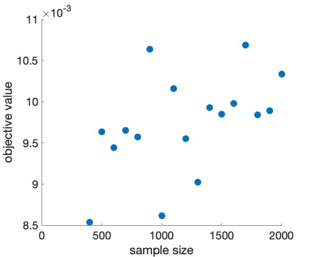
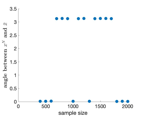
Figure 2: Results of the proposed algorithm in [10] on the phase retrieval problem (29). Left plot corresponds to the stationary values of the computed d-stationary points. Right plot corresponds to angles between the computed d-stationary points and $\bar{x}$. The initial points are all set to be in ${\cal D}^{\prime}$. It is clear that the angles are close to either $0$ and $\pi$.

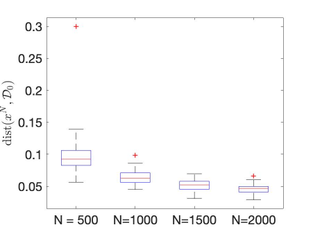
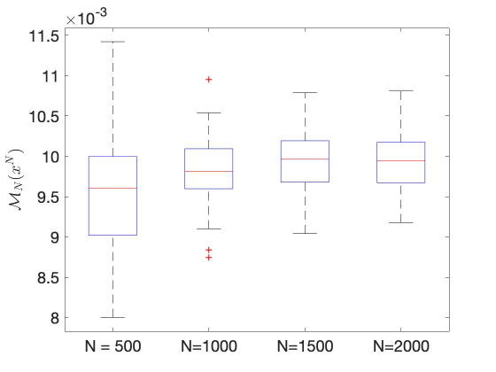
Figure 3: Boxplots of $\ell_{2}$ errors between computed d-stationary solutions and $\pm\bar{x}$ and ${\cal M}_{N}(x^{N})$ for various sample sizes. For each sample size, we repeat our simulation study for 100 times.

9 Concluding Remarks

Coupled nonconvex and nondifferentiable statistical estimation problems present great challenges for both rigorous computation and analysis. Understanding and differentiating properties of the computable solutions and establishing the asymptotics of their statistical behaviors are necessary tasks in addressing such challenges. Our paper offers a first step in this direction by analyzing the relationship between a sharp kind of stationary solutions of the empirical optimization problems and their population counterparts. There remains much to be done, such as the convergence rate and asymptotic distributions under relaxed assumptions and for general composite piecewise smooth estimation problems, refined connections between solutions of various kinds of the empirical problems and their analogs in the population formulations, and finally understanding the desirable merits and undesirable drawbacks of the stationary points and values obtained from numerical optimization algorithms in nonconvex estimation processes.

References

[1]H. Attouch.
Variational Convergence for Functions and Operators.
Pitman Press, Boston (1984).
[2]A.M. Bagirov, C. Clausen, and M. Kohler.
An algorithm for the estimation of a regression function by continuous piecewise linear functions.
Computational Optimization and Applications 45 (2010) 159–179.
[3]P. Bartlet and S. Mendelson.
Rademacher and Gaussian complexities: Risk bounds and structural results.
Journal of Machine Learning Research 3 (2002) 463–482.
[4]W. Bryc.
The Normal Distribution: Characterizations with Applications.
Springer Science & Business Media, 2012
[5]E.J. Candes, X. Li, M. Soltanolkotabi.
Phase retrieval via Wirtinger flow: Theory and algorithms.
IEEE Transactions on Information Theory 61 (2015) 1985–-2007.
[6]Y. Chen, Y. Chi, J. Fan and C. Ma.
Gradient descent with random initialization: fast global convergence for nonconvex phase retrieval.
Mathematical Programming 176 (2019) 5–37.
[7]H. Chernoff.
On the distribution of the likelihood ratio.
The Annals of Mathematical Statistics (1954) 573–578.
[8]K. Chung.
On a stochastic approximation method.
The Annals of Mathematical Statistics (1954) 463–483.
[9]F.H. Clarke.
Optimization and Nonsmooth Analysis.
Classics in Applied Mathematics.
SIAM, Volume 5, 1990.
[Reprint from John Wiley (New York 1983).]
[10]Y. Cui, J.S. Pang, and B. Sen.
Composite difference-max programs for modern statistical estimation problems.
SIAM Journal on Optimization 28 (2018) 3344–3374.
[11]Y. Cui, T.H. Chang, M. Hong and J.S. Pang.
A study of piecewise linear-quadratic programs.
arXiv:1709.05758 (2018).
[12]D. Dentcheva, S. Penev, and A. Ruszczynski.
Statistical estimation of composite risk functionals and
risk optimization problems.
Annals of the Institute of Statistical Mathematics 69 (2017) 737–760.
[13]D. Davis, D. Drusvyatskiy and C. Paquette.
The nonsmooth landscape of phase retrieval.
arXiv:1711.03247 (2018).
[14]J. Duchi and F. Ruan.
Solving (most) of a set of quadratic equalities: Composite optimization for robust phase retrieval.
Information and Inference: A Journal of the IMA 8 (2018) 471–529.
[15]J. Dupačová and R.J.-B. Wets.
Asymptotic behavior of statistical estimators and of optimal
solutions of stochastic optimization problems.
The Annals of Statistics 16 (1988) 1517–1549.
[16]D. Dunson and L.A. Hannah.
Multivariate convex regression with adaptive partitioning.
Journal of Machine Learning Research 14 (2013) 3261–3294.
[17]F. Facchinei and J.S. Pang.
Finite-dimensional Variational Inequalities and Complementarity Problems.
Springer, New York (2003).
[18]T.S. Ferguson.
A Course in Large Sample Theory. Routledge (1996).
[19]R.A. Fisher.
On the mathematical foundations of theoretical statistics.
Philosophical Transactions of the Royal Society A 222 (1922) 594–604 .
[20]R.A. Fisher.
Theory of statistical estimation.
Mathematical Proceedings of the Cambridge Philosophical Society 22 (1925) 700–725.
[21]C.J. Geyer.
On the asymptotics of constrained -estimation.
The Annals of Statistics 22 (1994) 1993–2010.
[22]X. Glorot, A. Bordes, and Y. Bengio.
Deep sparse rectifier neural networks.
In Proceedings of the 14th International Conference on Artificial Intelligence and Statistics (2011) 315–323.
[23]G. Gürkan, A. Yonca Özge and S. Robinson.
Sample-path solution of stochastic variational inequalities.
Mathematical Programming 84 (1999) 313–333.
[24]P.J. Huber.
The behavior of maximum likelihood estimates under nonstandard conditions.
Proceedings of the fifth Berkeley symposium on mathematical statistics and probability (1967)
Volume 1, Pages 221–233 University of California Press.
[25]C. Jin, L. Liu, R. Ge and M. Jordan.
On the local minima of the empirical risk.
In Proceedings of Neural Information Processing Systems (NIPS) 2018.
[26]A.J. King.
Asymptotic behaviour of solutions in stochastic optimization: nonsmooth analysis and the derivation of non-normal limit distributions.
Ph.D. dissertation, Department of Mathematics, University of Washington, Seattle (1993).
[27]A. King and R.T. Rockafellar.
Asymptotic theory for solutions in statistical estimation and stochastic programming.
Mathematics of Operations Research 18 (1993) 148–162.
[28]L. LeCam.
On the assumptions used to prove asymptotic normality of maximum likelihood estimates.
The Annals of Mathematical Statistics 41 (1970) 802–828.
[29]H.A. Le Thi and D.T. Pham.
The DC programming and DCA revised with DC models of real world nonconvex optimization problems.
Annals of Operations Research 133 (2005) 25–46.
[30]P.L. Loh and M. Wainwright.
High-dimensional regression with noisy and missing data: Provable guarantees with non-convexity.
The Annals of Statistics 40 (2012) 1637–1664.
[31]P.L. Loh and M. Wainwright.
Regularized M-estimators with nonconvexity: statistical and algorithmic theory for local optima.
Journal of Machine Learning Research 16 (2015) 559–616.
[32]P.L. Loh.
Statistical consistency and asymptotic normality for high-dimensional robust -estimators.
The Annals of Statistics 45 (2017) 866–896.
[33]Z. Lu, Z. Zhou and Z. Sun.
Enhanced proximal DC algorithms with extrapolation for a class of structured nonsmooth DC minimization.
Mathematical Programming 176 (2019) 369–401.
[34]J. Ma, J. Xu and A. Maleki.
Optimization-based AMP for phase retrieval: the impact of initialization and regularization.
IEEE Transactions on Information Theory 65 (2019) 3600–3629.
[35]S. Mei, Y. Bai and A. Montanari.
The landscape of empirical risk for non-convex losses.
The Annals of Statistics 46 (2018) 2747–2774.
[36]I. Molchanov.
Theory of Random Sets. Vol. 19, no. 2.
Springer, London (2005).
[37]A. Nemirovski, A. Juditsky, G. Lan and A. Shapiro.
Robust stochastic approximation approach to stochastic programming.
SIAM Journal on Optimization 19 (2009) 1574–1609.
[38]V. Nair and G.E. Hinton.
Rectified linear units improve restricted Boltzmann machines.
In Proceedings of the 27th International Conference on Machine Learning (2010) 807–814.
[39]J.S. Pang, M. Razaviyayn, and A. Alvarado.
Computing B-stationary points of nonsmooth DC programs.
Mathematics of Operations Research 42 (2016) 95–118.
[40]B. Polyak.
New stochastic approximation type procedures.
Avtomatica i Telemekhanika 7 (1990) 98–107.
[41]B. Polyak and A. Juditsky.
Acceleration of stochastic approximation by averaging.
SIAM Journal on Control and Optimization 30 (1992) 838–855.
[42]H. Robbins and S. Monro.
A stochastic approximation method.
Annals of Mathematical Statistics 22 (1951) 400–407.
[43]R.T. Rockafellar.
Convex Analysis.
Princeton University Press, Princeton (1970).
[44]R.T. Rockafellar and R.J.-B. Wets.
Variational Analysis. Springer, New York (1998).
[45]J. Royset.
Approximations of semicontinuous functions
with applications to stochastic optimization and statistical estimation.
Mathmeatical Programming, Series A, https://doi.org/10.1007/s10107-019-01413-z.
[46]J. Royset and R.J.-B. Wets.
Variational analysis of constrained M-estimators.
http://arxiv.org/abs/1702.08109v4 (May 2018).
[47]Y. Shechtman, Y. Eldar, O. Cohen, H. Chapman, J. Miao and M. Segev.
Phase retrieval with application to optical imaging: a contemporary overview.
IEEE signal processing magazine 32 (2015) 87–109.
[48]S. Scholtes.
Introduction to Piecewise Differentiable Equations.
Springer Briefs in Optimization (2002).
[49]S.G. Self and K.Y. Liang.
Asymptotic properties of maximum likelihood estimators and likelihood ratio tests under nonstandard conditions.
Journal of the American Statistical Association 82 (1987) 605–610.
[50]A. Shapiro.
Asymptotic properties of statistical estimators in stochastic programming.
The Annals of Statistics 17 (1989) 841–858.
[51]A. Shapiro.
Monte Carlo sampling methods.
In Rusczyński and Shapiro (eds.) Stochastic Programming, Handbooks in OR & MS.
Volume 10. Amsterdam: NorthHolland Publishing Company (2003).
[52]A. Shapiro, D. Dentcheva, and A. Ruszczyński.
Lectures on Stochastic Programming: Modeling and Theory.
SIAM Publications (Philadelphia 2009).
[53]A. Shapiro and H. Xu.
Uniform laws of large numbers for set-valued mappings and subdifferentials of random functions.
Journal of Mathematical Analysis and Applications 352 (2007) 1390–1399.
[54]A.W. van der Vaart.
Asymptotic Statistics
Vol. 3, Cambridge University Press (1998).
[55]A.W. van der Vaart and J. Wellner.
Weak Convergence and Empirical Processes
Springer Series in Statistics (1996).
[56]S. van de Geer.
Empirical Processes in M-estimation
vol. 6, Cambridge University Press (2000).
[57]H. Xu.
Sample average approximation methods for a class of stochastic variational inequality problems.
Asia-Pacific Journal of Operational Research 27 (2010) 103–119.
[58]H. Xu and D. Zhang.
Smooth sample average approximation of stationary points in nonsmooth stochastic optimization and applications.
Mathematical Programming 119 (2009) 371–401.
[59]A. Wald.
Note on the consistency of the maximum likelihood estimate.
The Annals of Mathematical Statistics 20 (1949) 595–601.
[60]G. Wang, G.B. Giannakis, and Y.C. Eldar.
Solving systems of random quadratic equations via truncated amplitude flow.
IEEE Transactions on Information Theory 64 (2018) 773–794.
[61]R.J.-B Wets.
A statistical approach to the solution of stochastic programs with (convex) simple recourse.
Working Paper, University of Kentucky (1979).
for small and affine
and
for small and affine
and