Ground-State Phase Diagram of an Anisotropic $S=1$ Ferromagnetic-Antiferromagnetic Bond-Alternating Chain

Abstract

By using mainly numerical methods, we investigate the ground-state phase diagram (GSPD) of an $S=1$ ferromagnetic-antiferromagnetic bond-alternating chain with the $XXZ$ and the on-site anisotropies. This system can be mapped onto an anisotropic spin-2 chain when the ferromagnetic interaction is much stronger than the antiferromagnetic interaction. Since there are many quantum parameters in this system, we numerically obtained the GSPD on the plane of the magnitude of the antiferromagnetic coupling versus its $XXZ$ anisotropy, by use of the exact diagonalization, the level spectroscopy as well as the phenomenological renormalization group. The obtained GSPD consists of six phases. They are the $XY$1, the large-$D$ (LD), the intermediate-$D$ (ID), the Haldane (H), the spin-1 singlet dimer (SD), and the Néel phases. Among them, the LD, the H, and the SD phases are the trivial phases, while the ID phase is the symmetry-protected topological phase. The former three are smoothly connected without any quantum phase transitions. It is also emphasized that the ID phase appears in a wider region compared with the case of the GSPD of the anisotropic spin-2 chain with the $XXZ$ and the on-site anisotropies. We also compare the obtained GSPD with the result of the perturbation theory.

I Introduction

In recent years, low dimensional quantum spin systems have been attracting increasing attention because they provide rich physics even when models are rather simple. Several years ago, we investigatedtone ; oka1 ; oka2 ; oka3 the $T=2$ quantum spin chain with the $XXZ$ and on-site anisotropies described by

$${\mathcal{H}}_{1}=\sum_{j}(T_{j}^{x}T_{j+1}^{x}+T_{j}^{y}T_{j+1}^{y}+\Delta T_{j}^{z}T_{j+1}^{z})+D_{2}\sum_{j}(T_{j}^{z})^{2},$$ (1)

where $T_{j}^{\mu}$ ($\mu=x,y,z$) represents the $\mu$-component of the spin-2 operator $\mbox{\boldmath$T$}_{j}$ at the $j$th site, and $\Delta$ and $D_{2}$ are, respectively, the $XXZ$ anisotropy parameter of the nearest-neighbor interactions and the on-site anisotropy parameter. We obtained the ground-state phase diagramtone ; oka1 (GSPD) mainly by the use of the exact diagonalization and the level spectroscopy (LS) analysisokamoto-ls ; nomura-ls ; kitazawa-ls ; nomura-kitazawa-ls . The remarkable features of the GSPD are: (a) there exists the intermediate-$D$ (ID) phase which was first predicted by Oshikawaoshikawa in 1992 and has been believed to be absent for about two decades until our findingtone ; oka1 ; oka2 in 2011; (b) the Haldane (H) state and the large-$D$ (LD) state belong to the same phase. These features are consistent with the discussion by Pollmann et al.pollmann2010 ; pollmann2012 . Namely, the ID state is a symmetry-protected topological (SPT) state protected by (i) the time-reversal symmetry $\mbox{\boldmath$S$}_{j}\to-\mbox{\boldmath$S$}_{j}$, as well as by (ii) the space inversion symmetry with respect to a bond, while the H state and the LD state are trivial states. Slightly after our works, the ID phase was also discussed by Tzeng tzeng and Kjäll et al. kjall .

Considering these situations, we investigate the GSPD of the $S=1$ ferromagnetic-antiferromagnetic bond-alternating chain, since it is thought that this chain can be mapped onto the spin-2 model in the strong ferromagnetic coupling limit. We describe our model in §2, and the numerically determined GSPD are shown in §3. In §4 the perturbation theory from the strong ferromagnetic coupling limit is developed. Section 5 is devoted to concluding remarks.

II Model

We investigate the model described by

$${\cal H}=\sum_{j}\{h^{\rm F}_{2j-1,2j}+h^{\rm AF}_{2j,2j+1}+D_{2}(S_{j}^{z})^{2}\}\,,$$ (2)

$$h^{\rm F}_{j,j^{\prime}}=-J_{\rm F}(S_{j}^{x}S_{j^{\prime}}^{x}+S_{j}^{y}S_{j^{\prime}}^{y}+\Delta_{\rm F}S_{j}^{z}S_{j^{\prime}}^{z})\,,$$ (3)

$$h^{\rm AF}_{j,j^{\prime}}=J_{\rm AF}(S_{j}^{x}S_{j^{\prime}}^{x}+S_{j}^{y}S_{j^{\prime}}^{y}+\Delta_{\rm AF}S_{j}^{z}S_{j^{\prime}}^{z})\,.$$ (4)

Here, $S_{j}^{\mu}$ ($\mu=x$, $y$, $z$) is the $\mu$-component of the spin-1 operator $\mbox{\boldmath$S$}_{j}$ acting on the $j$th site; $J_{\rm F}\,(>0.0)$ and $J_{\rm AF}\,(\geq 0.0)$ denote, respectively, the magnitudes of exchange interaction constants for the ferromagnetic and antiferromagnetic bonds; $\Delta_{\rm F}$ and $\Delta_{\rm AF}$ are, respectively, the parameters representing the $XXZ$ anisotropies of the former and latter interactions.

Figure 1: A sketch of the present model. Open circles denote $S=1$ spins. Solid and dotted lines are the ferromagnetic (F) and antiferromagnetic (AF) bonds, respectively.

III Ground-State Phase Diagram by Numerical Calculations

Since there are five parameters, $J_{\rm F}$, $J_{\rm AF}$, $\Delta_{\rm F}$, $\Delta_{\rm AF}$, and $D_{2}$, in our Hamiltonian (2), we restrict ourselves to the case where $J_{\rm F}=1.0$ (namely, $J_{\rm F}$ is the unit of energy), $\Delta_{\rm F}=0.8$, and $D_{2}=-1/30$, and numerically determine the GSPD on the $J_{\rm AF}$ versus $\Delta_{\rm AF}$ plane.

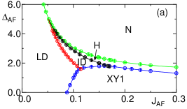
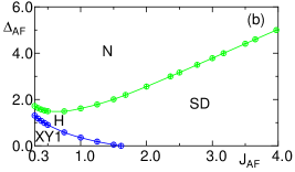
Figure 2: The GSPD on the $J_{\rm AF}$ versus $\Delta_{\rm AF}$ plane for the case of $J_{\rm F}=1.0$, $\Delta_{\rm F}=0.8$, and $D_{2}=-1/30$, obtained in the present work; (a) $0.0\leq J_{\rm AF}\leq 0.3$, (b) $0.3\leq J_{\rm AF}\leq 4.0$.

(a)       (b)

(c)       (d)

(e)

Figure 3: Physical pictures of the (a) LD, (b) H, (c) ID, (d) SD and (e) Néel states. Big circles denote $S=1$ spins, while small dots $S=1/2$ spins. Ellipses represent singlet pairs, whilst rectangles ferromagnetically coupled spin pairs or clusters. The namings of these states are based on the pictures of the $T=2$ spin system except for the SD state.

Figure 2 shows our GSPD on the $J_{\rm AF}$ versus $\Delta_{\rm AF}$ plane, which has been determined by using a variety of numerical methods based on the exact diagonalization calculation data. This GSPD consists of six phases, which are the $XY$1, LD, ID, H, spin-1 singlet dimer (SD), and Néel (N) phases. The physical pictures of latter five states are sketched in Fig.3. Among them, the LD, H, and SD phases are the trivial phases, while the ID phase is the SPT phase. Interestingly, the former three are smoothly connected without any quantum phase transitions between the LD and H phases and between the H and SD phases, and therefore they belong to the same phase. It is also emphasized that the ID phase appears in a wider region compared with the case of the GSPD of the Hamiltonian (1) tone ; oka1 ; oka2 .

We now explain how to determine numerically the phase boundary lines in the GSPD shown in Fig.2. We denote, respectively, by $E_{0}^{\rm P}(L,M)$ and $E_{1}^{\rm P}(L,M)$, the lowest and second-lowest energy eigenvalues of the Hamiltonian ${\cal H}$ under the periodic boundary condition within the subspace characterized by $N$ and $M$, where $N(=4$, $8$, $12$, $16)$ is the total number of spins in the system and $M(=0$, $\pm 1$, $\cdots$, $\pm N)$ is the total magnetization. We also denote by $E_{0}^{\rm T}(L,M,P)$ the lowest energy eigenvalue of ${\mathcal{H}}$ under the twisted boundary condition within the subspace characterized by $N$, $M$, and $P$, where $P(=+1$, $-1)$ is the eigenvalue of the space inversion operator with respect to the twisted bond. We numerically calculate these energies by means of the exact diagonalization method. In the following way, we evaluate the finite-size critical values of $J_{\rm AF}$ (or $\Delta_{\rm AF}$) for various values of $\Delta_{\rm AF}$ (or $J_{\rm AF}$) for each phase transition. Then, the phase boundary line for the transition is obtained by connecting the results for the $N\to\infty$ extrapolation of the finite-size critical values.

Firstly, the phase transition between the LD and ID phases and that between the ID and H phases are of the Gaussian type. Therefore, as is well known, the phase boundary lines can be accurately estimated by Kitazawa’s level spectroscopy (LS) method kitazawa-ls . Namely, we numerically solve the equation,

$$E_{0}^{\rm T}(N,0,+1)=E_{0}^{\rm T}(N,0,-1)$$ (5)

to calculate the finite-size critical values. It is noted that, at the $N\!\to\!\infty$ limit, $E_{0}^{\rm T}(N,0,+1)\!>\!E_{0}^{\rm T}(N,0,-1)$ in the ID phase and $E_{0}^{\rm T}(N,0,+1)\!<\!E_{0}^{\rm T}(N,0,-1)$ in the LD and H phases.

Secondly, the phase transitions between one of the LD, ID, H, and SD phases and the $XY$1 phase are of the Berezinskii-Kosterlitz-Thouless berezinskii ; kt ; kosterlitz type. Then, the phase boundary line can be accurately estimated by the LS method developed by Nomura and Kitazawa nomura-kitazawa-ls . Then, we solve the following equation to calculate the finite-size critical values:

$$E_{0}^{\rm P}(N,2)=E_{0}^{\rm T}(N,0,P)\,,$$ (6)

where $P\!=\!-1$ or $P\!=\!+1$ depending upon whether the transitions are associated with the ID phase or with the LD, H, and SD phases.

Lastly, since the phase transitions between one of the LD, H, SD phases and the N phase are the 2D Ising-type transition, the phase boundary line between these two phases can be estimated by the phenomenological renormalization group method nightingale . Then, the finite-size critical values for this transition are calculated by solving the equation,

$$N\,\Delta_{00}^{\rm P}(L,0)=(N+4)\,\Delta_{00}^{\rm P}(L+4,0)\,,$$ (7)

where $\Delta_{00}^{\rm P}(L,0)=E_{1}^{\rm P}(L,0)-E_{0}^{\rm P}(L,0)$.

IV Perturbation Theory from the Strong Ferromagnetic Coupling Limit

In the strong ferromagnetic coupling limit, it is thought that the present system can be mapped onto the spin-2 model. Here we take the unperturbed Hamiltonian as

$${\cal H}^{(0)}=\sum_{j}h^{\rm F(0)}_{2j-1,2j}\,,$$ (8)

$$h^{\rm F(0)}_{2j,2j+1}=-J_{\rm F}(S_{2j}^{x}S_{2j+1}^{x}+S_{2j}^{y}S_{2j+1}^{y}+S_{2j}^{z}S_{2j+1}^{z})\,.$$ (9)

The ground states of $h^{\rm F(0)}_{2j,2j+1}$ are five-fold degenerate, which are interpreted as isolated spin-2 states, expressed by the spin-2 operator $T$. We note that, if we include the $XXZ$ anisotropy in ${\cal H}^{(0)}$, we cannot treat lowest five states as isolated spin-2 states, In the lowest order perturbation theory, we obtain

$${\mathcal{H}}_{\rm eff}^{T=2}={J_{\rm AF}\over 4}\left\{\sum_{j}\left(T_{j}^{x}T_{j+1}^{x}+T_{j}^{y}T_{j+1}^{y}+\Delta_{\rm AF}T_{j}^{z}T_{j+1}^{z}\right)+\sum_{j}\left(\tilde{D}_{2}(T_{j}^{z})^{2}+\tilde{D}_{4}(T_{j}^{z})^{4}\right)\right\}\,,$$ (10)

$$\tilde{D}_{2}={14D_{2}-4\beta\over 3J_{\rm AF}}\,,$$ (11)

$$\tilde{D}_{4}=-{2D_{2}\over 3J_{\rm AF}}\,,$$ (12)

where

$$\beta\equiv J_{\rm F}(\Delta_{\rm F}-1).$$ (13)

It is interesting that $\tilde{D}_{4}(T_{j}^{z})^{4}$ term appears. Since we have set $\Delta_{\rm F}=0.8$, and $D_{2}=-1/30$, it holds

$$\tilde{D}_{2}={1\over 9J_{\rm AF}}\,,~{}~{}~{}~{}~{}\tilde{D}_{4}={1\over 45J_{\rm AF}}\,.$$ (14)

Unfortunately, the GSPD of the Hamiltonian (10) with the parameter set given by eq.(14) has not been reported in the literature. However, that with $\Delta_{\rm F}=0.8$, and $D_{2}=-1/15$ (namely, $-\tilde{D}_{2}=\tilde{D}_{4}=1/60J_{\rm AF}$) is shown in Fig.3(a) of our previous paperoka3 , Thus, as the second-best plan, we are going to compare our present GSPD with that in ref.oka3 . The GSPD of Fig.3(a) of oka3 can be recasted into Fig.4.

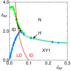
Figure 4: The GSPD obtained by the perturbation theory in case of $\Delta_{\rm F}=0.8$, and $D_{2}=-1/15$. The red dotted line is the result by mapping onto the $\sigma=1$ model, while other lines (black, blue and green) are that by mapping onto the $T=2$ model. If we combine these results around $J_{\rm AF}=0.05$, the numerically obtained GSPD (Fig.2) is qualitatively explained.

When the $XXZ$ anisotropy of the ferromagnetic interaction is introduced (namely, when $\beta\neq 0$), the five-fold degenerate states of ground states of $h^{\rm F(0)}_{2j,2j+1}$ are split into three levels with $T^{z}=0$, $T^{z}=\pm 1$ and $T^{z}=\pm 2$. We note that this effect is expressed as the $\tilde{D}_{2}(T_{j}^{z})^{2}$ and $\tilde{D}_{4}(T_{j}^{z})^{4}$ terms in the effective Hamiltonian (12). For our parameter set ($\beta=-0.2$ and $D_{2}=-1/30$), these energies are

$$E_{\rm on-site}\equiv J_{\rm AF}[\tilde{D}_{2}(T^{z})^{2}+\tilde{D}_{4}(T^{z})^{4}]=\begin{cases}0\,,&(T^{z}=0)\,,\\ J_{\rm AF}\displaystyle{\tilde{D}_{4}\left({\tilde{D}_{2}\over\tilde{D}_{4}}+1\right)}={2\over 15}\,,&(T^{z}=\pm 1)\,,\\ J_{\rm AF}\displaystyle{\tilde{D}_{4}\left(4{\tilde{D}_{2}\over\tilde{D}_{4}}+16\right)}={4\over 5}\,,&(T^{z}=\pm 2)\,.\end{cases}$$ (15)

When $J_{\rm AF}$ is much smaller than the splitting energy (for instance, $0.1$), the states with $T^{z}=\pm 2$ will be strongly suppressed. In this case, it is appropriate to neglect the $T^{z}=\pm 2$, which leads to the mapping onto the $\sigma=1$ spin system. A straightforward calculation leads to

$${\mathcal{H}}_{\rm eff}^{\sigma=1}={3\over 4J_{\rm AF}}\left\{\sum_{j}\left(\sigma_{j}^{x}\sigma_{j+1}^{x}+\sigma_{j}^{y}\sigma_{j+1}^{y}+{\Delta_{\rm AF}\over 3}\sigma_{j}^{z}\sigma_{j+1}^{z}\right)+{2\over 45J_{\rm AF}}\sum_{j}(\sigma^{z})^{2}\right\}.$$ (16)

The GSPD for the effective Hamiltonian (16) was obtained by Chen et al.chen . The LD (trivial) and Haldane (SPT) states of the GSPD of Chen et al. correspond to the LD (trivial) and ID (SPT) states of the GSPD of the present model, respectively. By recasting the GSPD of Chen et al. leads to the red dotted line in Fig.4. Thus, Fig.4 quantitatively explains our numerical result shown in Fig.2.

V Concluding Remarks

We have investigated the GSPD of an $S=1$ ferromagnetic-antiferromagnetic bond-alternating chain with the $XXZ$ and the on-site anisotropies by using mainly numerical methods. In the GSPD, there appear the $XY$1, the large-$D$ (LD), the intermediate-$D$ (ID), the Haldane (H), the spin-1 singlet dimer (SD), and the Néel phases. Among them, the LD, the H, and the SD phases are the trivial phases, while the ID phase is the SPT phase. We have also developed the perturbation theory from the strong ferromagnetic coupling limit to map onto the $T=2$ effective model, which quantitatively explains the numerically obtained GSPD.

We can see a considerably wider region of the ID phase in Fig.2 than that for the model described by the Hamiltonian (1), in which the ID phase was numerically observed for the first time. The reason for the wider ID region in Fig.2 is the existence of the $\tilde{D}_{4}(T_{j}^{z})^{4}$ term in eq.(10). We have already shown that the addition of the $D_{4}(T_{j}^{z})^{4}$ term with $D_{4}>0$ to the Hamiltonian (1) drastically widen the ID region oka3 . We believe that the finding of the wider ID region in our GSPD provides a guiding principle to find or synthesize real materials in which the ID phase could be experimentally observed.

References

- (1) T. Tonegawa, K. Okamoto, H. Nakano, T. Sakai, K. Nomura, and M. Kaburagi: J. Phys. Soc. Jpn. 80, 043001 (2011).
- (2) K. Okamoto, T. Tonegawa, H. Nakano, T. Sakai, K. Nomura, and M. Kaburagi: J. Phys.: Conf. Ser. 302, 012014 (2011).
- (3) K. Okamoto, T. Tonegawa, H. Nakano, T. Sakai, K. Nomura, and M. Kaburagi: J. Phys.: Conf. Ser. 320, 012018 (2011).
- (4) K. Okamoto, T. Tonegawa, T. Sakai, and M. Kaburagi: JPS Conf. Proc. 3, 014022 (2014).
- (5) K. Okamoto and K. Nomura: Phys. Lett. A 169, 433 (1992).
- (6) K. Nomura and K. Okamoto: J. Phys. A: Math. Gen. 27, 5773 (1994).
- (7) A. Kitazawa: J. Phys. A: Math. Gen. 30, L285 (1997).
- (8) K. Nomura and A. Kitazawa: J. Phys. A: Math. Gen. 31, 7341 (1998)
- (9) M. Oshikawa: J. Phys.: Condens. Matter 4, 7469 (1992).
- (10) F. Pollmann, A. M. Turner, E. Berg, and M. Oshikawa: Phys. Rev. B 81, 064439 (2010).
- (11) F. Pollmann, E. Berg, A. M. Turner, and M. Oshikawa: Phys. Rev. B 85, 075125 (2012).
- (12) Y.-C. Tzeng: Phys. Rev. B 86, 024403 (2012).
- (13) J. A. Kjäll, M. P. Zaletel, R. S. K. Mong, J. H. Bardarson, and F. Pollmann: Phys. Rev. B 87, 235106 (2013).
- (14) V. L. Berezinskii, Zh. Eksp. Teor. Fiz. 59, 907 (1970) [Sov. Phys. JETP 32, 493 (1971)]; 61,1144 (1971) [Sov. Phys. JETP 34, 610 (1971)].
- (15) J. M. Kosterlitz and D. J. Thouless, J. Phys. C: Solid State Phys. 6, 1181 (1973).
- (16) J. M. Kosterlitz, J. Phys. C: Solid State Phys. 7, 1046 (1974).
- (17) P. Nightingale: Physica A 83 (1976) 561.
- (18) W. Chen, K. Hida and C. Sanctuary, Phys. Rev. B 67, 104401 (2003).