Distributed filtered hyperinterpolation for noisy data on the sphere

Abstract

Problems in astrophysics, space weather research and geophysics usually need to analyze noisy big data on the sphere. This paper develops distributed filtered hyperinterpolation for noisy data on the sphere, which assigns the data fitting task to multiple servers to find a good approximation of the mapping of input and output data. For each server, the approximation is a filtered hyperinterpolation on the sphere by a small proportion of quadrature nodes. The distributed strategy allows parallel computing for data processing and model selection and thus reduces computational cost for each server while preserves the approximation capability compared to the filtered hyperinterpolation. We prove quantitative relation between the approximation capability of distributed filtered hyperinterpolation and the numbers of input data and servers. Numerical examples show the efficiency and accuracy of the proposed method.

68Q32, 65D05, 41A50, 33C55, 65T60

1 Introduction

In cosmic microwave background analysis, global ionospheric prediction to geomagnetic storms, climate change modelling, environment governance and meteorology and remote sensing, data are collected on the sphere and usually big and noisy [1, 13, 14, 29, 32, 37]. One of critical tasks of big data analysis on the sphere is to find an effective data fitting strategy to approximate the mapping between input and output data. There have been many useful methods for fitting spherical data, for example approximations by spherical harmonics [33], spherical basis functions [22, 23, 19, 35], spherical wavelets [13], spherical needlets [2, 34, 12, 20, 28, 43], spherical kernel methods [11, 25] and spherical filtered hyperinterpolation [40]. When noise is sufficiently small and decreases with size of data, least squares regularization can be used to reduce noise in learning representation, see e.g. [22, 19]. This method is however not suitable when the size of noisy data is large, as then the regularization condition implies that noise must be close to zero. In this paper, we propose a new strategy based on distributed learning — distributed filtered hyperintepolation, which assigns the data fitting task to multiple servers then synthesizes them as a global prediction model.

Spherical filtered hyperinterpolation, developed by Sloan and Womersley [39, 40], is a constructive approach: given degree $L$ (which indicates the level of precision), use $N$ data on the sphere to find a filtered expansion of spherical harmonics up to degree $2L$. The filtering strategy uses an appropriate filter and the data at nodes of a quadrature rule. When the quadrature rule that is a set of pairs of points on the sphere and real weights is exact for numerical integration of polynomials up to degree $(c+1)L$ (see the definition of (4)), the filtered hyperinterpolation reaches the best polynomial approximation [40, 41]. The computational cost is thus determined by the number $N$ of data, which has at least order $\mathcal{O}\left(L^{2}\right)$ [18]. The cost becomes heavy as degree $L$ or the number of data increases. One way to reduce the computational burden is to distribute the approximation task to multiple servers, each of which works on a fraction of the total computation using a small proportion of all data, and then synthesize the computed fitting models of all servers to produce a global predictor. To achieve that, we apply distributed learning strategy [26, 27] to spherical filtered hyperinterpolation, which leads to distributed filtered hyperinterpolation (DFH).

The proposed DFH can fit $N$ noisy data $y_{i}=f^{*}(\mathbf{x}_{i})+\epsilon_{i}$, $i=1,\dots,N$, for continuous function $f^{*}$ on the sphere, and independent bounded noises $\epsilon_{i}$. We show that the approximation error of DFH for such noisy data depends on the number of data and the smoothness of the target function $f^{*}$. We also consider the DFH with independent random interpolation points, which we call distributed filtered hyperinterpolation with random sampling, and prove that for distributions of the random points satisfying appropriate conditions, DFH has the same approximation capability as that with “deterministic” quadrature rule.

The rest of the paper is organized as follows. In Section 2, we introduce filtered kernel, quadrature rule and “ordinary” spherical filtered hyperinterpolation. In Section 3, we define distributed filtered hyperinterpolation with “deterministic” quadrature rule and give the relation of its approximation error and numbers of data and servers. Section 4 defines the distributed filtered hyperinterpolation with random sampling and gives its error estimate. Section 5 gives the numerical examples of the distributed filtered hyperinterpolation where we study the impact of the numbers of data, servers and noise on approximation error. Section 6 gives the proofs for the main results.

2 Filtered Kernel, Quadrature Rule and Filtered Hyperinterpolation

In this section, we introduce the spherical filtered hyperinterpolation defined by filtered kernels and quadrature rule.

2.1 Filtered kernels

For $d\geq 2$, let $\mathbf{x}\cdot\mathbf{y}$ be the inner product of two points $\mathbf{x},\mathbf{y}$ in $\mathbb{R}^{d+1}$, and the Euclidean norm $|\mathbf{x}|:=\sqrt{\mathbf{x}\cdot\mathbf{x}}$. Let $\mathbb{S}^{d}:=\{\mathbf{x}\in\mathbb{R}^{d+1}:|\mathbf{x}|=1\}$ be the unit sphere of $\mathbb{R}^{d+1}$. The $\mathbb{S}^{d}$ is a compact metric space with geodesic distance

$$\mbox{dist}(\mathbf{x},\mathbf{y}):=\arccos(\mathbf{x}\cdot\mathbf{y}),\quad\mathbf{x},\mathbf{y}\in\mathbb{S}^{d}$$

as the metric. For $1\leq p<\infty$, let $L_{p}(\mathbb{S}^{d})$ be the real-valued $L_{p}$ space on $\mathbb{S}^{d}$ with Lebesgue measure $\omega:=\omega_{d}$ and $L_{p}$ norm $\|f\|_{L_{p}(\mathbb{S}^{d})}:=\left(\int_{\mathbb{S}^{d}}|f(\mathbf{x})|^{p}\mathrm{d}\omega(\mathbf{x})\right)^{1/p}$ for $f\in L_{p}(\mathbb{S}^{d})$. In particular, $L_{2}(\mathbb{S}^{d})$ is a Hilbert space with inner product

$$\langle f,g\rangle_{L_{2}(\mathbb{S}^{d})}:=\int_{\mathbb{S}^{d}}f(\mathbf{x})g(\mathbf{x})\mathrm{d}\omega(\mathbf{x}),\quad f,g\in L_{p}(\mathbb{S}^{d}).$$

Denote by $L_{\infty}(\mathbb{S}^{d})$ the space of all real-valued continuous functions on $\mathbb{S}^{d}$ with uniform norm $\|f\|_{L_{\infty}}:=\max_{\mathbf{x}\in\mathbb{S}^{d}}|f(\mathbf{x})|$. The volume of $\mathbb{S}^{d}$ is

$$|\mathbb{S}^{d}|:=\omega_{d}(\mathbb{S}^{d}):=\frac{2\pi^{\frac{d+1}{2}}}{\Gamma(\frac{d+1}{2})}.$$

For $\ell\in\mathbb{N}_{0}:=\{0,1,\dots\}$, the restriction to $\mathbb{S}^{d}$ of a homogeneous harmonic polynomial of degree $\ell$ is called a spherical harmonic of degree $\ell$. Let $\mathbb{H}^{d}_{\ell}$ be the space of all spherical harmonics of degree $\ell$, and for $L\in\mathbb{N}_{0}$, $\Pi_{L}^{d}$ the space of all spherical polynomials of degree up to $L$. Then, $\Pi_{L}^{d}=\bigoplus_{\ell=0}^{L}\mathbb{H}_{\ell}^{d}$. The dimension of $\mathbb{H}^{d}_{\ell}$ is

$$Z_{d,\ell}:=\mbox{dim}\ \mathbb{H}^{d}_{\ell}=\left\{\begin{array}[]{ll}\displaystyle\frac{2\ell+d-1}{\ell+d-1}{{\ell+d-1}\choose{\ell}},&\ell\geq 1,\\[5.69054pt] 1,&\ell=0,\end{array}\right.$$

and then the dimension of $\Pi_{L}^{d}$ is $\sum_{\ell=0}^{L}Z_{d,\ell}=Z_{d+1,L}{\asymp}L^{d}$. Here for two sequences $a_{\ell}$ and $b_{\ell}$, $\ell\in\mathbb{N}_{0}$, $a_{\ell}\asymp b_{\ell}$ means that there exists constants $c,c^{\prime}$ such that $c^{\prime}b_{\ell}\leq a_{\ell}\leq cb_{\ell}$ for all $\ell\in\mathbb{N}_{0}$. The Laplace-Beltrami operator $\Delta^{*}$ on $\mathbb{S}^{d}$ has the eigenfunctions $Y_{\ell,m}$ and eigenvalues $\lambda_{\ell}:=\ell(\ell+d-1)$, $\ell\in\mathbb{N}_{0}$, $m=1,\dots,Z_{d,\ell}$:

$$\Delta^{*}Y_{\ell,m}=\lambda_{\ell}Y_{\ell,m}.$$

Let $P_{\ell}^{(d+1)}(t)$, $t\in[-1,1]$, be the normalized Gegenbauer polynomial which satisfies $P_{\ell}^{(d+1)}(1)=1$ and the orthogonality relation

$$\int_{-1}^{1}P_{\ell}^{(d+1)}(t)P_{\ell^{\prime}}^{(d+1)}(t)(1-t^{2})^{\frac{d-2}{2}}\mathrm{d}t=\frac{|\mathbb{S}^{d}|}{|\mathbb{S}^{d-1}|Z_{d,\ell}}\delta_{\ell,\ell^{\prime}},$$

where $\delta_{\ell,\ell^{\prime}}$ is the Kronecker symbol. Let $\eta:[0,\infty)\rightarrow\mathbb{R}$ be a filter with specified smoothness $\kappa\geq 1$ satisfying

(1) $$\eta\in C^{\kappa}(\mathbb{R}_{+});\quad\mbox{supp}\>\eta\subseteq[1/2,2];\quad{\eta(t)^{2}+\eta(2t)^{2}}=1\ \mbox{for}\ t\in[1/2,1].$$

The filtered kernel $K_{n}(\mathbf{x}\cdot\mathbf{x}^{\prime})$, $n\geq 1$, is then given by

(2) $$K_{n}(\mathbf{x}\cdot\mathbf{x}^{\prime})=\sum_{\ell=0}^{\infty}\eta\left(\frac{\ell}{n}\right)\frac{Z_{d,\ell}}{|\mathbb{S}^{d}|}P_{\ell}^{(d+1)}(\mathbf{x}\cdot\mathbf{x}^{\prime}),$$

see [34]. The approximation property of the filtered kernel depends on the smoothness of the filter $\eta$. We refer readers to e.g. [40, P.101] for examples of filtered kernels satisfying (1). Since the support of $\eta$ is in $[1/2,2]$, $K_{n}(\mathbf{x}\cdot\mathbf{y})$ is a polynomial of either $\mathbf{x}$ or $\mathbf{y}$ of degree up to $2n-1$.

2.2 Spherical quadrature rules

The geometric properties of a finite set $X_{N}:=\{\mathbf{x}_{1},\dots,\mathbf{x}_{N}\}$, $N\geq 2$, of points on $\mathbb{S}^{d}$ can be described by mesh norm, separation radius and mesh ratio, as we introduce now. The mesh norm (or covering radius) of $X_{N}$ is

$$h(X_{N}):=\max_{\mathbf{x}\in\mathbb{S}^{d}}\min_{\mathbf{x}_{i}\in X_{N}}\mbox{dist}(\mathbf{x},\mathbf{x}_{i}).$$

The mesh norm is the minimal radius with which the caps with centers at points of $X_{N}$ covers $\mathbb{S}^{d}$. The separation radius of $X_{N}$ is

$$\delta(X_{N}):=\frac{1}{2}\min_{j\neq k}\mbox{dist}(\mathbf{x}_{j},\mathbf{x}_{k}).$$

This is half the smallest geodesic distance between any pair of points in $X_{N}$. The mesh ratio of $X_{N}$ is the minimum of distances between points of $X_{N}$:

$$\rho(X_{N}):=\frac{h(X_{N})}{\delta(X_{N})}\geq 1,$$

which measures how uniformly the points of $X_{N}$ are distributed on $\mathbb{S}^{d}$. We say a sequence of point sets $\{X_{N}\}_{N=2}^{\infty}$ $\tau$-quasi uniform, if there is a constant $\tau\geq 2$ such that $\rho(X_{N})\leq\tau$ for all $N\geq 2$. The existence of a $\tau$-quasi uniform sequence of points sets is proved in [35]. Assume the sequence of points sets $\{X_{N}\}_{N=2}^{\infty}$ is $\tau$-quasi uniform, then

(3) $${h(X_{N})}\leq\tau\delta(X_{N})\leq\frac{\tau}{2N^{1/d}}.$$

It then follows from (3) and [24, Lemma 2] that

$$\mathbb{S}^{d}\subseteq\bigcup_{\mathbf{x}_{i}\in X_{N}}\mathcal{C}(\mathbf{x}_{i},\tau/(2N^{1/d}))\ \ \mbox{and}\ \ \max_{\mathbf{x}_{i}\in X_{N}}\left|X_{N}\bigcap\mathcal{C}(\mathbf{x}_{i},\tau/(2N^{1/d}))\right|\leq 2\pi^{d-1}\tau^{d},$$

where $|A|$ is the cardinality of the finite set $A$ and $\mathcal{C}(\mathbf{x},r):=\{\mathbf{y}\in\mathbf{S}^{d}:\mbox{dist}(\mathbf{x},\mathbf{y})\leq r\}$ the spherical cap with center $\mathbf{x}$ and radius $r$, $r>0$.

We say a set $\mathcal{Q}_{N}:=\{(w_{i},\mathbf{x}_{i}):w_{i}\in\mathbb{R}\hbox{~{}and~{}}\mathbf{x}_{i}\in\mathbb{S}^{d},i=1,\dots,N\}$, $N\geq 2$, a quadrature rule on $\mathbb{S}^{d}$, where $w_{i}$ are called weights of $\mathcal{Q}_{N}$. For $L\geq 0$, a quadrature rule $\mathcal{Q}_{N}$ is said to be exact for polynomials of degree up to $L$ if

(4) $$\int_{\mathbb{S}^{d}}P(\mathbf{x})\mathrm{d}\omega(\mathbf{x})=\sum_{i=1}^{N}w_{i}P(\mathbf{x}_{i})\quad\forall P\in\Pi_{L}^{d}.$$

The following lemma gives a sequence of polynomial-exact quadrature rules whose point sets are $\tau$-quasi uniform, see [7, Theorem 3.1] and also [31].

Lemma 2.1 ([7, 31]).

If $\{X_{N}\}_{N=2}^{\infty}$ is $\tau$-quasi uniform, then for $N\geq 2$, there exist positive weights $w_{i}$, $i=1,\dots,N$, such that $0\leq w_{i}\leq c_{2}N^{-1}$ and

$$\int_{\mathbb{S}^{d}}P(\mathbf{x})\mathrm{d}\omega(\mathbf{x})=\sum_{\mathbf{x}_{i}\in X_{N}}w_{i}P(\mathbf{x}_{i})\quad\forall P\in\Pi_{c_{3}N^{1/d}}^{d},$$

where $c_{2}$ and $c_{3}$ are constants depending only on $\tau$ and $d$.

For $1\leq p<\infty$, let $L_{p,\mu}:=L_{p}(\mathbb{S}^{d},\mu)$ be the $L_{p}$ space on $\mathbb{S}^{d}$ with respect to a probability measure $\mu$, endowed with norm $\|f\|_{p,\mu}:=\left(\int_{\mathbb{S}^{d}}|f(\mathbf{x})|^{p}\mathrm{d}\mu(\mathbf{x})\right)^{1/p}$. The following theorem shows that if $X_{N}=\{\mathbf{x}_{i}\}_{i=1}^{N}\subset\mathbb{S}^{d}$ is a set of i.i.d. random points with distribution $\mu$, then with high probability, the quadrature rule is exact for polynomials with a specific degree.

Theorem 2.2.

Let $X_{N}=\{\mathbf{x}_{i}\}_{i=1}^{N}$ be i.i.d. random points on $\mathbb{S}^{d}$ with distribution $\mu$ which satisfies

(5) $$\|f\|_{L_{1}(\mathbb{S}^{d})}\leq c_{4}\|f\|_{1,\mu}\quad\forall f\in L_{1}(\mathbb{S}^{d})\cap L_{1,\mu}$$

for a positive absolute constant $c_{4}$. Then, for integer $N$ satisfying $N/n^{2d}>c$ for a sufficiently large constant $c$, there exits a quadrature rule $\mathcal{Q}_{N}:=\{(\mathbf{x}_{i},w_{i,n})\}_{i=1}^{N}$ such that

$$\int_{\mathbb{S}^{d}}P_{n}(\mathbf{x})\mathrm{d}\mu(\mathbf{x})=\sum_{i=1}^{N}w_{i,n}P_{n}(\mathbf{x}_{i})\quad\forall P_{n}\in\Pi_{n}^{d}$$

holds, and $\sum_{i=1}^{N}|{w_{i,n}}|^{2}\leq\frac{2}{{N}}$ and $w_{i,n}\geq 0$ for all $i=1,\dots,N$, with confidence at least $1-4\exp\left\{-CN/n^{d}\right\}$, where $C$ is a constant depending only on $c_{4}$ and $d$.

We give the proof of Theorem 2.2 in Section 6. The confidence level in Theorem 2.2 is exponential of $n$ and $N$, which is different from polynomial confidence level given by [21, Theorem 4.1]. This exponential relation plays a crucial role in error estimation for the distributed filtered hyperinterpolation for spherical noisy data. It is also different from [25] in that the established quadrature rule satisfying (5) holds with positive weights. The condition of the distribution in (5) describes the distortion of $\mu$ from the uniform distribution on $\mathbb{S}^{d}$ that is also the spherical Lebesgue measure. The probabilistic quadrature rule in Theorem 2.2 is critical to the construction of distributed filtered hyperinterpolation with random sampling (see Section 4.2).

2.3 Spherical filtered hyperinterpolation approximation

Using filtered kernel and quadrature rule, we define the spherical filtered hyperinterpolation, as follows.

Definition 2.3 ([40]).

Let $d\geq 2$ and $1\leq p\leq\infty$. For $f\in L_{p}(\mathbb{S}^{d})$, the filtered hyperinterpolation (approximation) with a quadrature rule $\mathcal{Q}_{N}:=\{(w_{i},\mathbf{x}_{i})\}_{i=1}^{N}$ is

(6) $$V_{n,N}(f;\mathbf{x}):=\sum_{i=1}^{N}w_{i}f(\mathbf{x}_{i})K_{n}(\mathbf{x}_{i}\cdot\mathbf{x}),\quad n\geq 1.$$

The approximation property of the filtered hyperinterpolation depends on the smoothness of the function space. For $r\in\mathbb{R}_{+}$, let

$$b_{\ell}^{r}:=(1+\lambda_{\ell})^{r/2}\asymp(1+\ell)^{r}.$$

Let $\{Y_{\ell,m}:\ell=0,1,\dots,\>m=1,\dots,Z_{d,\ell}\}$ be an orthonormal basis for the space $L_{2}(\mathbb{S}^{d})$, and

$$\widehat{f}_{\ell m}:=\langle f,Y_{\ell,m}\rangle_{L_{2}(\mathbb{S}^{d})}:=\int_{\mathbb{S}^{d}}f(\mathbf{x})Y_{\ell m}(\mathbf{x})\mathrm{d}\omega(\mathbf{x})$$

the Fourier coefficients of $f\in L_{2}(\mathbb{S}^{d})$. For $d\geq 2$, $1\leq p\leq\infty$ and $r\in\mathbb{R}_{+}$, the Sobolev space $\mathbb{W}_{p}^{r}(\mathbb{S}^{d})$ is the space of functions $f$ satisfying $\sum_{\ell=0}^{\infty}b_{\ell}^{r}\widehat{f}_{\ell m}Y_{\ell,m}\in L_{p}(\mathbb{S}^{d})$, endowed with the norm $\|f\|_{\mathbb{W}^{r}_{p}(\mathbb{S}^{d})}:=\left\|\sum_{\ell=0}^{\infty}b_{\ell}^{r}\widehat{f}_{\ell m}Y_{\ell,m}\right\|_{L_{p}(\mathbb{S}^{d})}$.

The following lemma, which is proved by Wang and Sloan [41], shows the relation of the approximation error of the filtered hyperinterpolation approximation $V_{n,N}$ and the smoothness of the function space under the condition that the associated quadrature rule is exact for polynomials of degree up to $3n-1$.

Lemma 2.4 ([41]).

Let $d\geq 2$, $1\leq p\leq\infty$ and $r>d/p$. Let $V_{n,N}$ be the filtered hyperinterpolation in (6) with quadrature rule $\mathcal{Q}_{N}$ exact for polynomials of degree up to $3n-1$ and with the filter $\eta$ in $C^{\kappa}(\mathbb{R}_{+})$, $\kappa\geq\left\lfloor\frac{d+3}{2}\right\rfloor$. Then, for $f\in\mathbb{W}_{p}^{r}(\mathbb{S}^{d})$,

(7) $$\|f-V_{n,N}(f)\|_{L_{p}(\mathbb{S}^{d})}\leq c_{5}\>n^{-r}\|f\|_{\mathbb{W}_{p}^{r}(\mathbb{S}^{d})},$$

where $c_{5}$ depends only upon $d,p,r$ and $\eta$. The order $n^{-r}$ in (7) is optimal.

3 Distributed Filtered Hyperinterpolation with Deterministic Sampling

A data set $D=\{(\mathbf{x}_{i},y_{i})\}_{i=1}^{|D|}$ on $\mathbb{S}^{d}$ is a set of pairs of points $\Lambda_{D}:=\{\mathbf{x}_{i}\}_{i=1}^{|D|}$ on the sphere and real numbers $y_{i}$. Elements of $D$ are called data. The points $\mathbf{x}_{i}$ of $\Lambda_{D}$ are called the sampling points of $D$. To distinguish quadrature rule with random points which we will investigate later, we say a data set $D$ has deterministic sampling for (fixed) sampling points. In this section, we introduce a new filtered hyperinterpolation for which distributed learning can be used. The data $y_{i}$ are the values of a function $f^{*}$ on $\mathbb{S}^{d}$ plus noise, that is,

(8) $$y_{i}=f^{*}(\mathbf{x}_{i})+\epsilon_{i},\quad\mathbf{E}[\epsilon_{i}]=0,\quad|\epsilon_{i}|\leq M\quad\forall i=1,\dots,|D|.$$

The $D$ satisfying (8) is then called noisy data set associated with $f^{*}$.

3.1 Filtered hyperinterpolation for noisy data: deterministic sampling

We first study the performance of the filtered hyperinterpolation for a noisy data set $D$ whose data are stored on a “big enough” machine.

Definition 3.1.

For $s\in\mathbb{N}_{0}$ and $\{\mathbf{x}_{i}\}_{i=1}^{|D|}$, let $\mathcal{Q}_{|D|}$ be the quadrature rule given by Lemma 2.1, which is exact for polynomials of degree up to $s$ and has positive weights $\{w_{i,s,D}\}_{i=1}^{|D|}$ satisfying $0\leq w_{i,s,D}\leq c_{2}|D|^{-1}$. The filtered hyperinterpolation for noisy data associated with a function $f^{*}$ on $\mathbb{S}^{d}$ is

(9) $$f^{\diamond}_{D,n}(x):=\sum_{i=1}^{|D|}w_{i,s,D}\>y_{i}K_{n}(\mathbf{x}_{i}\cdot\mathbf{x}),$$

where $K_{n}$ is a filtered kernel in (2) for $\eta\in C^{\kappa}(\mathbb{R}_{+})$ with $\kappa\geq\left\lfloor\frac{d+3}{2}\right\rfloor$ and $n\leq s$.

The kernel $K_{n}$ provides a smoothing method for the function $f^{*}$ using data $D$. As we shall see below, the approximation error of this filtered hyperterpolation has the convergence rate depending on the smoothness of function $f^{*}$.

If $\Lambda_{D}$ is $\tau$-quasi uniform, it then follows from Lemma 2.1 that $s=c_{3}N^{1/d}$. We do not assume the magnitude of the noise extremely small, the filter $\eta$ of the filtered kernel $K_{n}$ shall then be chosen properly to minimize the impact of noise on interpolation. This is a problem similar to “model selection” in the statistical and machine learning [9]. To say it precisely, if the support $n$ is too large, then the filtered hyperinterpolation $f^{\diamond}_{D,n}$ will have precise approximation at the data set $\{(\mathbf{x}_{i},y_{i})\}_{i=1}^{D}$, but $f^{\diamond}_{D,n}$ may not be a good approximation of $f^{*}$ due to the noise. If the support is too small, the performance of the filtered hyperinterpolation $f^{\diamond}_{D,n}(\mathbf{x}_{i})$ is not good, even at the interpolation points. It is then preferable to set $n$ as a parameter in the training process. For $\Lambda_{D}$, the quadrature rule in Definition 3.1 (which is from Lemma 2.1) is valid for $n$ sufficiently large. The parameter selection thus needs only a few steps of computation, while the filtered hyperterpolation in Definition 3.1 allows us to handle massive noisy spherical data. This property of filtered hyperinterpolation is different from other algorithms such as the regularized least squares [19]: the latter needs to compute the inverse of the kernel matrix for each regularization parameter.

The following theorem shows that the filtered hyperinterpolation $f^{\diamond}_{D,n}$ can approximate $f^{*}$ well, provided that the support of the filtered kernel is appropriately tuned and the sampling point set $\Lambda_{D}$ is $\tau$-quasi uniform for $\tau\geq 2$.

Theorem 3.2.

Let $d\geq 2$ and $r>d/2$. Assume the sampling point set $\Lambda_{D}$ of the data set $D$ is $\tau$-quasi uniform for $\tau\geq 2$, and $\frac{c_{3}}{6}|D|^{1/(2r+d)}\leq n\leq\frac{c_{3}}{3}|D|^{1/(2r+d)}$ for constant $c_{3}$ in Lemma 2.1. Then, the filtered hyperinterpolation $f_{D,n}^{\diamond}$ for noisy data set $D$ with target function $f^{*}\in\mathbb{W}_{2}^{r}(\mathbb{S}^{d})$ satisfies

(10) $$\mathbf{E}\left\{\|f^{\diamond}_{D,n}-f^{*}\|_{L_{2}(\mathbb{S}^{d})}^{2}\right\}\leq C_{1}|D|^{-2r/(2r+d)},$$

where $C_{1}$ is a constant independent of $|D|$ and $n$.

Remark 3.3.

Here the condition $r>d/2$ is the embedding condition such that any function in $\mathbb{W}_{2}^{r}(\mathbb{S}^{d})$ has a representation of a continuous function on $\mathbb{S}^{d}$. The numerical computation of the filtered hyperinterpolation then makes sense.

We give the proof of Theorem 3.2 in Section 6. As mentioned above, since $\Lambda_{D}$ is $\tau$-quasi uniform, the quadrature rule for the filtered hyperinterpolation in Definition 3.1 is exact for $\Pi_{s}^{d}$ with $s=c|D|^{1/d}$. As we choose $n\leq c|D|^{1/(2r+d)}\leq s$ in Theorem 3.2, $f^{\diamond}_{D,n}$ reproduces polynomials in $\Pi_{s}^{d}$. Theorem 3.2 illustrates that if the scattered data $\Lambda_{D}$ has good geometric property, for example, $\tau$-quasi uniformity, and the support of the filter $\eta$ is appropriately chosen, then the spherical filtered hyperinterpolation for noisy data set $D$ can approximate a sufficiently smooth target function on the sphere in high precision in probablistic sense. By [17], the rate $|D|^{-2r/(2r+d)}$ in (10) cannot be essentially improved in the scenario of (8). Thus, Theorem 3.2 provides a feasibility analysis of the spherical filtered hyperinterpolation for spherical data with random noise.

3.2 Distributed filtered hyperinterpolation: deterministic sampling

We say a large data set $D$ is distributively stored on $m$ local machines if for $j=1,\dots,m$, $m\geq 2$, the $j$th machine contains a subset $D_{j}$ of $D$, and there is no common data between any pair of machines, that is, $D_{j}\cap D_{j^{\prime}}=\emptyset$ for $j\neq j^{\prime}$, and $D=\cup_{j=1}^{m}D_{j}$. The data sets $D_{1},\dots,D_{m}$ are called distributed data sets of $D$. In this case, the filtered hyperinterpolation $f^{\diamond}_{D,n}$ which needs access to the entire data set $D$ is infeasible. Instead, in this section, we construct a distributed filtered hyperinterpolation for the distributed data sets $\{D_{j}\}_{j=1}^{m}$ of $D$ by the divide and conquer strategy [26].

Definition 3.4.

The distributed filtered hyperinterpolation $\overline{f^{\diamond}_{D,n}}$ for distributed data sets $\{D_{j}\}_{j=1}^{m}$ of a noisy data set $D$ associated with function $f^{*}$ on $\mathbb{S}^{d}$ is a synthesized estimator of local estimators $f^{\diamond}_{D_{j},n}$, $j=1,2,\dots,m$, each of which is the spherical filtered hyperinterpolation (9) for noisy data set $D_{j}$:

(11) $$\overline{f^{\diamond}}(\{D_{j}\}_{j=1}^{m},n;\mathbf{x}):=\overline{f^{\diamond}_{D,n}}(\mathbf{x}):=\sum_{j=1}^{m}\frac{|D_{j}|}{|D|}f^{\diamond}_{D_{j},n}(\mathbf{x}),\quad{\bf x}\in\mathbb{S}^{d}.$$

The synthesis here is a process when the local estimators communicate to a central processor to produce the global estimator $\overline{f^{\diamond}_{D,n}}$.

The following theorem shows that the distributed filtered hyperinterpolation $\overline{f^{\diamond}_{D,n}}$ has similar approximation performance as $f^{\diamond}_{D,n}$ if the number of local machines is not large.

Theorem 3.5.

Let $d\geq 2$, $r>d/2$, $m\geq 2$ and $D$ a noisy data set satisfying (8). Let $\{D_{j}\}_{j=1}^{m}$ be $m$ distributed data sets of $D$. For $j=1,\dots,m$, the sampling point set $\Lambda_{D_{j}}$ of $D$ is $\tau$-quasi uniform for $\tau\geq 2$. If the distributed filtered hyperinterpolation $\overline{f^{\diamond}_{D,n}}$ for $\{D_{j}\}_{j=1}^{m}$ satisfies that the target function $f^{*}$ is in $\mathbb{W}_{2}^{r}(\mathbb{S}^{d})$, $\frac{c_{3}}{6}|D|^{1/(2r+d)}\leq n\leq\frac{c_{3}}{3}|D|^{1/(2r+d)}$ for constant $c_{3}$ in Lemma 2.1, and $\min_{j=1,\dots,m}|D_{j}|\geq|D|^{\frac{d}{2r+d}}$, then,

(12) $$\mathbf{E}\left\{\|\overline{f^{\diamond}_{D,n}}-f^{*}\|_{L_{2}(\mathbb{S}^{d})}^{2}\right\}\leq C_{2}|D|^{-2r/(2r+d)},$$

where $C_{2}$ is a constant independent of $|D|$, $|D_{1}|,\dots,|D_{m}|$ and $n$.

Remark 3.6.

The condition $\min_{j=1,\dots,m}|D_{j}|\geq|D|^{\frac{d}{2r+d}}$ has a close connection to the number $m$ of local machines. In particular, if $|D_{1}|=\dots=|D_{m}|$, since each $D_{j}$ is $\tau$-quasi uniform, $\min_{j=1,\dots,m}|D_{j}|\geq|D|^{\frac{d}{2r+d}}$ is equivalent to $m\leq|D|^{\frac{2r}{2r+d}}$.

The proof of Theorem 3.5 is postponed in Section 6. Theorem 3.5 illustrates that if $\min_{j=1,\dots,m}|D_{j}|\geq|D|^{\frac{d}{2r+d}}$, then with the same assumption as Theorem 3.2, the distributed filtered hyperinterpolation will have the same approximation performance as the filtered hyperinterpolation that treats all the distributed data sets as a whole “big enough” machine.

4 Distributed Filtered Hyperinterpolation with Random Sampling

We say a data set $D$ has random sampling if its sampling points are i.i.d. random points on $\mathbb{S}^{d}$. In this section, we construct a filtered hyperinterpolation for noisy data satisfying (8) with random sampling points.

4.1 Filtered hyperinterpolation for noisy data: random sampling

The filtered hyperinterpolation for noisy data with random sampling can be constructed as follows. Let $D=\{(\mathbf{x}_{i},y_{i})\}_{i=1}^{|D|}$ and $n\in\mathbb{N}$. Let the quadrature rule $\mathcal{Q}_{|D|}:=\{(a^{*}_{i,n,D},\mathbf{x}_{i})\}_{i=1}^{|D|}$ as given by Theorem 2.2, which is exact for polynomials of degree $n$. For $m\geq 2$, let

(13) $$a_{i,n,D}=\left\{\begin{array}[]{ll}a^{*}_{i,n,D},&\displaystyle\mbox{if}\ \sum_{i=1}^{|D|}|a^{*}_{i,n,D}|^{2}\leq 2/m,\\[2.84526pt] 0,&\mbox{otherwise},\end{array}\right.\quad\forall i=1,\dots,|D|.$$

Definition 4.1.

The filtered hyperinterpolation for noisy data $D:=\{(\mathbf{x}_{i},y_{i})\}_{i=1}^{|D|}$ with random sampling points $\{\mathbf{x}_{i}\}_{i=1}^{|D|}$ is

(14) $$f_{D,n}(\mathbf{x}):=\sum_{i=1}^{|D|}a_{i,n,D}\>y_{i}K_{n}(\mathbf{x}_{i}\cdot\mathbf{x}).$$

The following theorem gives the approximation error of the filtered hyperinterpolation in Definition 4.1 for sufficiently smooth functions.

Theorem 4.2.

Let $d\geq 2$ and $r>d/2$. Let the noisy data set $D$ with i.i.d. random sampling points on $\mathbb{S}^{d}$ and distribution $\mu$ satisfying (5). For integer $n$ satisfying $\frac{c_{3}}{6}|D|^{1/(2r+d)}\leq n\leq\frac{c_{3}}{3}|D|^{1/(2r+d)}$ with constant $c_{3}$ in Lemma 2.1, the filtered hyperinterpolation $f_{D,n}$ for noisy data set $D$ with target function $f^{*}\in\mathbb{W}_{2}^{r}(\mathbb{S}^{d})$ has the approximation error

(15) $$\mathbf{E}\left\{\|f_{D,n}-f^{*}\|_{L_{2}(\mathbb{S}^{d})}^{2}\right\}\leq C_{3}|D|^{-2r/(2r+d)},$$

where $C_{3}$ is a constant independent of $|D|$.

We give the proof of Theorem 4.2 in Section 6. Theorems 3.2 and 4.2 show that the filtered hypinterpolation approximations with random sampling and deterministic sampling achieve the same optimal convergence rate.

4.2 Distributed filtered hyperinterpolation: random sampling

The distributed filtered hyperinterpolation with random sampling is a weighted average of filtered hyperinterpolation approximations for data on local machines. Here the weight for a local machine is the proportion of the data used by the machine to all data. Let $f_{D_{j},n}$ be the filtered hyperinterpolation for data $D_{j}$. Similar as (11), the global estimator $\overline{f}_{D,n}$ is defined as follows.

Definition 4.3.

Let $d\geq 2$ and $D$ a noisy data set satisfying (8). The sampling points of $D$ are i.i.d random points on $\mathbb{S}^{d}$. For $m\geq 2$, let $\{D_{j}\}_{j=1}^{m}$ be $m$ distributed data sets of $D$, and for $j=1,\dots,m$, $f_{D_{j},n}$ be the filtered hyperinterpolation for $D_{j}$ given by Definition 4.1. The distributed filtered hyperinterpolation for distributed data sets $\{D_{j}\}_{j=1}^{m}$ of $D$ is

(16) $$\overline{f}_{D,n}:=\sum_{j=1}^{m}\frac{|D_{j}|}{|D|}f_{D_{j},n}.$$

The $f^{*}$ in (8) is called target function to $\overline{f}_{D,n}$.

The following theorem gives an upper bound of approximation error for distributed filtered hyperinterpolation with random sampling.

Theorem 4.4.

Let $d\geq 2$, $r>d/2$, $m\geq 2$ and $D$ a noisy data set satisfying (8). The sampling points are i.i.d random points on $\mathbb{S}^{d}$ with distribution $\mu$ in (5). If the target function $f^{*}\in\mathbb{W}_{2}^{r}(\mathbb{S}^{d})$, $\frac{c_{3}}{6}|D|^{1/(2r+d)}\leq n\leq\frac{c_{3}}{3}|D|^{1/(2r+d)}$ with constant $c_{3}$ in Lemma 2.1, and $\min_{j=1,\dots,m}|D_{j}|\geq|D|^{\frac{d+\nu}{2r+d}}$ for some $\nu$ in $(0,2r)$, then,

(17) $$\mathbf{E}\left\{\|\overline{f}_{D,n}-f^{*}\|_{L_{2}(\mathbb{S}^{d})}^{2}\right\}\leq C_{4}|D|^{-2r/(2r+d)},$$

where $C_{4}$ is a constant independent of $|D|$, $|D_{1}|,\dots,|D_{m}|$ and $n$.

The proof of Theorem 4.4 will be given in Section 6. From Theorems 4.4 and 3.5, we see that the distributed filtered hyperinterpolation approximations with random sampling and deterministic sampling can both achieve the convergence rate of order $|D|^{-2r/(2r+d)}$. To achieve this approximation order, the condition on the number of local machines of the random sampling is stronger than the deterministic case, since the former requires $\min_{j=1,\dots,m}|D_{j}|\geq|D|^{(d+\nu)/(2r+d)}$ for $\nu\in(0,2r)$, while the latter only needs $\min_{j=1,\dots,m}|D_{j}|\geq|D|^{d/(2r+d)}$.

Here we only consider error estimates with respect to Lebesgue measure. It would be interesting to consider error estimates for distributed learning with respect to other measures as done in [50, 49, 51].

5 Numerical Examples

(a) $f$

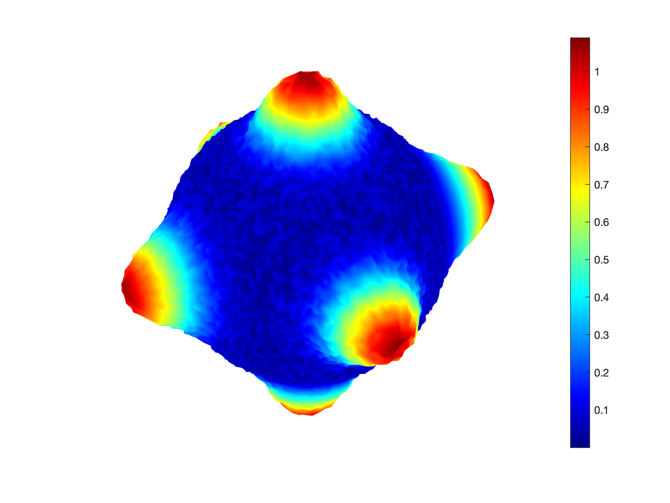
(b) $f$ plus noise

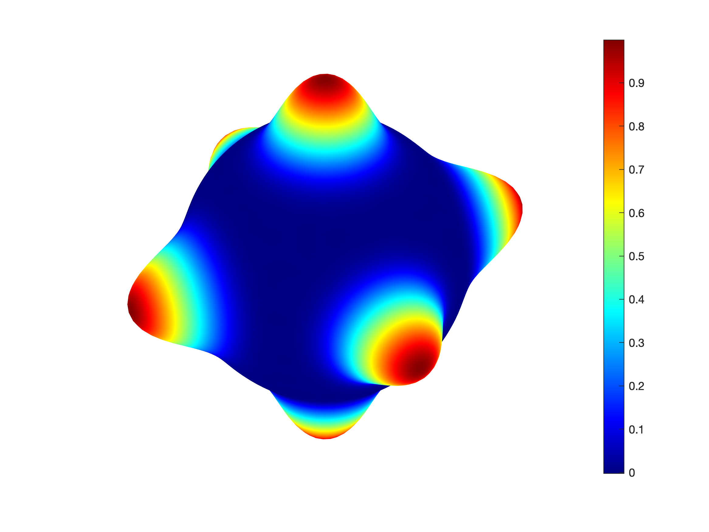
(c) $\overline{f^{\diamond}_{D,n}}$

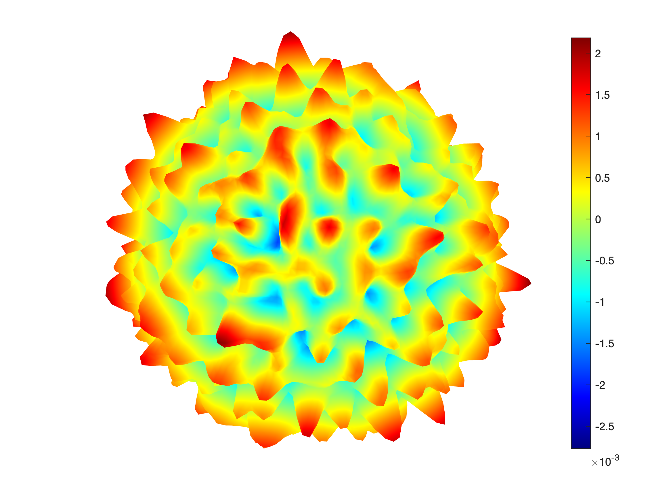
(d) Error

Figure 1: (a) Function $f$ in (18) which is in Sobolev space $H^{4.5}(\mathbb{S}^{2})$; (b) Noisy data $f+\epsilon$ with noise level $\sigma=0.1$; (c) Distributed filtered hyperinterpolation $\overline{f^{\diamond}_{D,n}}$ with $n=25$, $m=100$, $\sigma=0.1$ and the noisy dataset $D$ given on the nodes of symmetric spherical $75$-design; (d) Error $\overline{f^{\diamond}_{D,n}}-f$.

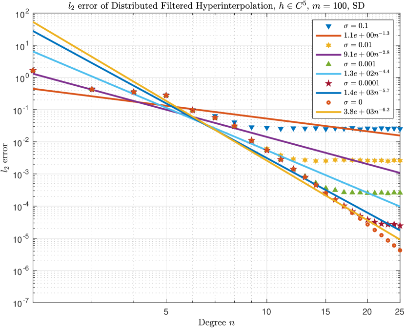
Figure 2: Errors v.s. degree $n$ for distributed filtered hyperinterpolation, $n\leq 25$, $m=100$, $\sigma=0,0.0001,0.001,0.01,0.1$.

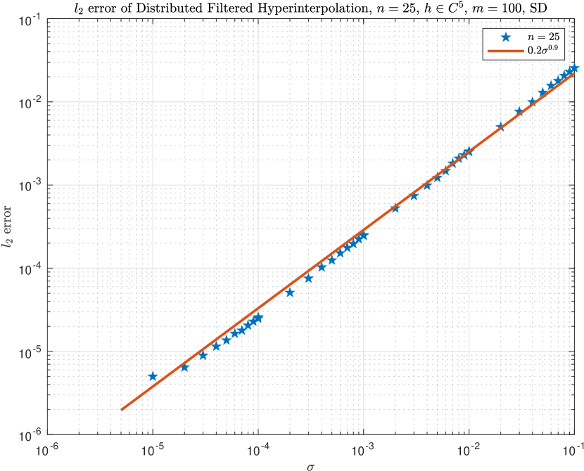
Figure 3: Errors v.s. standard variance $\sigma$ for distributed filtered hyperinterpolation, $n=25$, $m=100$

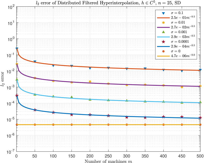
Figure 4: Errors v.s. number of machines $m$ for distributed filtered hyperinterpolation, $n=25$, $m\leq 500,\sigma=0,0.0001,0.001,0.01,0.1$

In this section, we test distributed filtered hyperinterpolation on noisy data on $\mathbb{S}^{2}$. We use Womersley’s symmetric spherical $t$-designs [46, 10] as quadrature rule for distributed filtered hyperinterpolation. The symmetric spherical $t$-design is an equal-weighted quadrature with $\mathcal{O}\left(t^{2}\right)$ nodes satisfying (4) for degree $n\leq t$, where the order $\mathcal{O}\left(t^{2}\right)$ is optimal as a consequence of [4].

Let $(u)_{+}:=\max\{u,0\}$ for $u\in\mathbb{R}$. The normalised Wendland-Wu function is given by

$$\phi(u):=\widetilde{\phi}\left(\frac{8u}{15\sqrt{\pi}}\right),\quad u\in\mathbb{R},$$

where $\widetilde{\phi}(u)$ is the original Wendland-Wu function

$$\widetilde{\phi}(u):=(1-u)_{+}^{8}(32u^{3}+25u^{2}+8u+1).$$

See [8, 45, 48]. The $\phi({\bf x}\cdot{\bf z})\in H^{4.5}(\mathbb{S}^{2})$ is a radial basis function on the sphere $\mathbb{S}^{2}$ with centre at ${\bf z}\in\mathbb{S}^{2}$ [23, 36]. We then define

(18) $$f({\bf x}):=\sum_{i=1}^{6}\phi({\bf x}\cdot{\bf z}_{i})$$

which is the linear combination of radial basis functions $\phi({\bf x}\cdot{\bf z}_{i})$ with centres at ${\bf z}_{1}=(1,0,0)$, ${\bf z}_{2}=(-1,0,0)$, ${\bf z}_{3}=(0,1,0)$, ${\bf z}_{4}=(0,-1,0)$, ${\bf z}_{5}=(0,0,1)$, ${\bf z}_{6}=(0,0,-1)$. The smoothness of $f$ is $4.5$, i.e. $f\in H^{4.5}(\mathbb{S}^{2})$. We use the function $f$ plus Gaussian white noise as the noisy data. That is, at each node ${\bf x}_{i}\in\mathbb{S}^{2}$,

(19) $$y_{i}=f({\bf x}_{i})+\epsilon,\quad\epsilon\sim N(0,\sigma^{2}),$$

where ${\bf x}_{i}$ are the nodes of a symmetric spherical $t$-design and $\sigma\geq 0$.

Figures 1a and b show the pictures of $f$ and a realisation of $f+\epsilon$ with noise level $\sigma=0.1$. Figure 1c shows the distributed filtered hyperinterpolation approximation $\overline{f^{\diamond}_{D,n}}$ of degree $n=25$ for noisy data $y_{i}$. The distributed filtered hyperinterpolation uses $m=100$ machines and $C^{5}$-filter $\eta$ [42, 43, 44] which satisfies the condition of smoothness of filter in Theorem 3.5. On the $j$-th machine, $j=1,\dots,100$, the filtered hyperinterpolation uses a $3n=75$-design with $2,852$ nodes, where the design is rotated from Womersley’s symmetric spherical $75$-design [46] by the rotation matrix

$$\rho_{j}:=\begin{pmatrix}\cos(\theta_{j})&-\sin(\theta_{j})&0\\ \sin(\theta_{j})&\cos(\theta_{j})&0\\ 0&0&1\end{pmatrix}$$

with $\theta_{j}=j\pi/m$. The rotated spherical design satisfies the same polynomial exactness property for numerical integration as the unrotated symmetric spherical design since the rotation of a spherical design is still a spherical design with the same separation and filling radii [5, 6, 15]. The distributed filtered hyperinterpolation then satisfies the condition of Theorem 3.5, which uses $285,200$ points in total. The function values are evaluated at $10,000$ generalized spiral points on $\mathbb{S}^{2}$, which are equally-distributed points [3, 38]. Figure 1d shows the approximation error of $\overline{f^{\diamond}_{D,n}}$ to $f$, which illustrates that errors are small compared to the magnitude of the function $f$.

Figure 2 shows the convergence rate (with respect to $n$) of the approximation error of the distributed filtered hyperinterpolation for $y_{i}$ with noise standard variance $\sigma=0,0.0001,0.001,0.01,0.1$. It illustrates that the approximation rate increases as the noise level becomes higher (i.e. when $\sigma$ is larger). When $\sigma=0$ and then the data is not contaminated by noise, the approximation error reaches the highest convergence rate at order $n^{-6.7}$. The convergence rate of the distributed filtered hyperinterpolation is higher than the upper bound of Theorem 3.5, since the function $f$ is sufficiently smooth.

Figure 3 shows that the approximation error of the distributed filtered hyperinterpolation of degree $n=25$ with $m=100$ machines converges at the rate $0.2\sigma^{0.9}$ with decrease of noise level $\sigma$. The noise level of data impacts the approximation precision of distributed filtered hyperinterpolation.

Figure 4 illustrates the impact of the number $m$ of machines on approximation capability as we can see for a noise level $\sigma>0$, the approximation error converges at rate around $m^{-0.5}$. This means that the noise level changes the absolute magnitude of approximation error but has little impact on the trend of approximation rate with the increase of number of machines.

6 Proofs

6.1 Proof for Theorem 2.2

Theorem 2.2 uses the norming set method [31] to derive the probabilistic quadrature rule. To prove Theorem 2.2, we need the following four lemmas. The first one is the Nikolskiî inequality on the sphere, which was proved in [30].

Lemma 6.1.

Let $1\leq p<q\leq\infty,$ $n\geq 1$ be an integer, and $P\in\Pi_{n}^{d}$. Then

$$\|P\|_{L^{q}(\mathbb{S}^{d})}\leq\tilde{C}_{1}n^{\frac{d}{p}-\frac{d}{q}}\|P\|_{L^{p}(\mathbb{S}^{d})},$$

where the constant $\tilde{C}_{1}>0$ depends only on $d,p,q$.

The second one is the following concentration inequality, which was established in [47].

Lemma 6.2.

Let $\mathcal{G}$ be a set of functions on compact metric space $Z$. For every $g\in\mathcal{G}$, if $|g-\mathbf{E}g|\leq B$ almost everywhere and $\mathbf{E}(g^{2})\leq\tilde{c}(\mathbf{E}g)^{\alpha}$ for some $B\geq 0$, $0\leq\alpha\leq 1$ and $\tilde{c}\geq 0$. Then, for any $\varepsilon>0$,

$$\mathbf{P}\left\{\sup_{g\in\mathcal{G}}\frac{\left|\mathbf{E}g-\frac{1}{m}\sum_{i=1}^{m}g(z_{i})\right|}{\sqrt{(\mathbf{E}g)^{\alpha}+\varepsilon^{\alpha}}}>\varepsilon^{1-\frac{\alpha}{2}}\right\}\leq 2\mathcal{N}(\mathcal{G},\varepsilon)\exp\left\{-\frac{m\varepsilon^{2-\alpha}}{2(\tilde{c}+\frac{1}{3}B\varepsilon^{1-\alpha})}\right\},$$

where $\mathcal{N}(\mathcal{G},\varepsilon)$ denotes the covering number [47] of $\mathcal{G}$ with radius $\varepsilon$.

The third one is a covering number estimate for Banach spaces, as given in [52].

Lemma 6.3.

Let $\mathbb{B}$ be a finite-dimensional Banach space. Let $B_{R}$ be the closed ball of radius $R$ centered at the origin given by $B_{R}:=\{f\in\mathbb{B}:\|f\|_{\mathbb{B}}\leq R\}$. Then,

$$\log\mathcal{N}(B_{R},\varepsilon)\leq\dim(\mathbb{B})\log\left(\frac{4R}{\varepsilon}\right).$$

To state the last lemma, we need following definitions. Let $\mathcal{X}$ be a finite dimensional vector space with norm $\|\cdot\|_{\mathcal{X}}$, and $\mathcal{Z}\subset\mathcal{X}^{*}$ be a finite set. We say that $\mathcal{Z}$ is a norm generating set for $\mathcal{X}$ if the mapping $T_{\mathcal{Z}}:\mathcal{X}\rightarrow\mathbb{R}^{|\mathcal{Z}|}$ defined by $T_{\mathcal{Z}}(x)=(z(x))_{z\in\mathcal{Z}}$ is injective, and $T_{\mathcal{Z}}$ is called the sampling operator. Let $W:=T_{\mathcal{Z}}(\mathcal{X})$ be the range of $T_{\mathcal{Z}}$, then the injectivity of $T_{\mathcal{Z}}$ implies that $T_{\mathcal{Z}}^{-1}:W\rightarrow\mathcal{X}$ exists. Let $\|\cdot\|_{\mathbb{R}^{|\mathcal{Z}|}}$ be the norm of $\mathbb{R}^{|\mathcal{Z}|}$ norm, and $\|\cdot\|_{\mathbb{R}^{|\mathcal{Z}|^{*}}}$ the dual norm on $\mathbf{R}^{|\mathcal{Z}|^{*}}$ for $\|\cdot\|_{\mathbb{R}^{|\mathcal{Z}|}}$. Equipping $W$ with the induced norm, and let $\|T_{\mathcal{Z}}^{-1}\|:=\|T_{\mathcal{Z}}^{-1}\|_{W\rightarrow\mathcal{X}}.$ In addition, let $\mathcal{K}_{+}$ be the positive cone of $\mathbb{R}^{|\mathcal{Z}|}$ which is the set of all $(r_{z})_{z\in\mathcal{Z}}\in\mathbb{R}^{|\mathcal{Z}|}$ such that $r_{z}\geq 0$. Then the following lemma [31] holds.

Lemma 6.4.

Let $\mathcal{Z}$ be a norm generating set for $\mathcal{X}$, with $T_{\mathcal{Z}}$ the corresponding sampling operator. If $g\in\mathcal{X}^{*}$ with $\|g\|_{\mathcal{X}^{*}}\leq\mathcal{A}$, then there exist positive numbers $\{a_{z}\}_{z\in\mathcal{Z}}$, depending only on $g$ such that for every $x\in\mathcal{X},$

$$g(x)=\sum_{z\in\mathcal{Z}}a_{z}z(x),$$

and

$$\|(a_{z})\|_{\mathbb{R}^{|\mathcal{Z}|^{*}}}\leq\mathcal{A}\|T_{\mathcal{Z}}^{-1}\|.$$

Also, if $W$ contains an interior point $v_{0}\in\mathcal{K}_{+}$ and if $g(T_{\mathcal{Z}}^{-1}v)\geq 0$ when $v\in W\cap\mathcal{K}_{+}$, then we may choose $a_{z}\geq 0.$

We are ready to prove Theorem 2.2.

Proof 6.5 (Proof of Theorem 2.2).

For $p=1,2$, without loss of generality, we prove Theorem 2.2 for $P_{n}\in\Pi_{n}^{d}$ satisfying $\|P_{n}\|_{p,\mu}=A$ for some constant $A>0$. For an arbitrary $P_{n}\in\Pi_{n}^{d}$ with $\|P_{n}\|_{p,\mu}=A$, it follows from (5) and Lemma 6.1 that

$$\|P_{n}\|_{L_{\infty}(\mathbb{S}^{d})}\leq\tilde{C}_{1}n^{\frac{d}{p}}\|P_{n}\|_{L_{p}(\mathbb{S}^{d})}\leq c^{1/p}_{4}\tilde{C}_{1}n^{\frac{d}{p}}\|P_{n}\|_{p,\mu},$$

and

$$\mathbf{E}\left\{|P_{n}|^{2p}\right\}=\int_{\mathbb{S}^{d}}|P_{n}(\mathbf{x})|^{2p}{\rm d}\mu(\mathbf{x})\leq\|P_{n}\|^{p}_{L_{\infty}(\mathbb{S}^{d})}\int_{\mathbb{S}^{d}}|P_{n}(\mathbf{x})|^{p}{\rm d}\mu(\mathbf{x})\leq c_{4}(\tilde{C}_{1})^{p}n^{d}\|P_{n}\|^{p}_{p,\mu}\mathbf{E}\left[|P_{n}|^{p}\right].$$

Let $Z=\mathbb{S}^{d}$, $g(z_{i})=|P_{n}(\mathbf{x}_{i})|^{p}$, $B=2c_{4}(\tilde{C}_{1})^{p}n^{d}A^{p}$, $\tilde{c}=c_{4}(\tilde{C}_{1})^{p}n^{d}A^{p}$, $m=N$, $\alpha=1$ and $\mathcal{G}_{p}=\{|P_{n}|^{p}:P_{n}\in\Pi_{n}^{d},\|P_{n}\|_{p,\mu}=A\}$ in Lemma 6.2. Then, for any $\varepsilon>0$,

$$\mathbf{P}\left\{\sup_{P_{n}\in\Pi_{n}^{d},\|P_{n}\|_{p,\mu}=A}\frac{\left|\|P_{n}\|_{p,\mu}^{p}-\frac{1}{N}\sum_{i=1}^{N}|P_{n}(\mathbf{x}_{i})|^{p}\right|}{\sqrt{\|P_{n}\|_{p,\mu}^{p}+\varepsilon}}>\sqrt{\varepsilon}\right\}$$

$$\quad\leq 2\mathcal{N}(\mathcal{G}_{p},\varepsilon)\exp\left\{-\frac{{N}\varepsilon}{\tilde{C}_{2}n^{d}A^{p}}\right\},$$

where $\tilde{C}_{2}=10c_{4}(\tilde{C}_{1})^{p}/3$. For $p=1$, we have $|P_{n}|-|P_{n}^{*}|\leq|P_{n}-P_{n}^{*}|$ for any $P_{n},P_{n}^{*}\in\Pi_{n}^{d}$. Then, it follows from the definition of the covering number that $\mathcal{N}(\mathcal{G}_{1},\varepsilon)\leq\mathcal{N}(\mathcal{G}_{1}^{\prime},\varepsilon)$, where $\mathcal{G}_{1}^{\prime}:=\{P_{n}\in\Pi_{n}^{d}:\|P_{n}\|_{p,\mu}=A\}$. For $p=2$, $|P_{n}|^{2}\in\Pi_{2n}^{d}$. Let $\mathcal{G}_{2}^{\prime}:=\{P_{n}\in\Pi_{2n}^{d}:\|P_{n}\|_{p,\mu}=A\}$. Then, $\mathcal{N}(\mathcal{G}_{2},\varepsilon)=\mathcal{N}(\mathcal{G}_{2}^{\prime},\varepsilon)$. It then follows from Lemma 6.3 that for $p=1,2$,

$$\mathbf{P}\left\{\sup_{P_{n}\in\Pi_{n}^{d},\|P_{n}\|_{p,\mu}=A}\frac{\left|\|P_{n}\|_{p,\mu}^{p}-\frac{1}{N}\sum_{i=1}^{N}|P_{n}(\mathbf{x}_{i})|^{p}\right|}{\sqrt{\|P_{n}\|_{p,\mu}^{p}+\varepsilon}}>\sqrt{\varepsilon}\right\}$$

$$\quad\leq 2\exp\left\{(2n)^{d}\log\frac{4A^{p}}{\varepsilon}-\frac{{N}\varepsilon}{\tilde{C}_{2}n^{d}A^{p}}\right\},$$

where we use $\dim\mathcal{G}_{p}\leq(pn)^{d}$ for $p=1,2$. Let $\varepsilon=A^{p}/4$. As $N/n^{d}>c$ for a sufficiently large $c>0$,

$$(2n^{d})\log\frac{4A^{p}}{\varepsilon}<\frac{N\varepsilon}{\tilde{C}_{2}n^{d}A^{p}}.$$

Then, with confidence

(20) $$1-2\exp\left\{-\tilde{C}_{3}N/n^{d}\right\},$$

there holds

$$\left|\|P_{n}\|_{p,\mu}^{p}-\frac{1}{N}\sum_{i=1}^{N}|P_{n}(\mathbf{x}_{i})|^{p}\right|\leq\sqrt{\varepsilon(\|P_{n}\|^{p}_{p,\mu}+\varepsilon)}=\frac{\sqrt{5}}{4}\|P_{n}\|^{p}_{p,\mu}.$$

Then, with the same confidence as (20),

(21) $$\frac{1}{3}\|P_{n}\|_{p,\mu}^{p}\leq\frac{1}{N}\sum_{i=1}^{N}|P_{n}(\mathbf{x}_{i})|^{p}\leq\frac{5}{3}\|P\|_{p,\mu}^{p}\quad\forall P_{n}\in\Pi_{n}^{d},\ p=1,2.$$

Now, we use (21) with $p=2$ and Lemma 6.4 to prove Theorem 2.2. In Lemma 6.4, we take $\mathcal{X}=\Pi_{n}^{d}$, $\|P_{n}\|_{\mathcal{X}}=\|P_{n}\|_{2,\mu}$, and $\mathcal{Z}$ to be the set of point evaluation functionals $\{\delta_{\mathbf{x}_{i}}\}_{i=1}^{N}$. The operator $T_{\mathcal{Z}}$ is then the restriction map $P_{n}\mapsto P_{n}|_{X_{N}}$ and

$$\|f\|_{X_{N},2}:=\left(\frac{1}{N}\sum_{i=1}^{N}|f(\mathbf{x}_{i})|^{2}\right)^{\frac{1}{2}}.$$

It follows from (21) that with confidence at least

$$1-2\exp\left\{-\tilde{C}_{3}N/n^{d}\right\},$$

there holds $\|T_{\mathcal{Z}}^{-1}\|\leq\sqrt{\frac{5}{3}}$. We take $g$ to be the functional

$$g:P_{n}\mapsto\int_{\mathbb{S}^{d}}P_{n}(x)\mathrm{d}\mu(x).$$

By Hölder inequality, $\|g\|_{\mathcal{X}^{*}}\leq 1$. Lemma 6.4 then shows that there exists a set of real numbers $\{w_{i,n}\}_{i=1}^{N}$ such that

$$\int_{\mathbb{S}^{d}}P_{n}(x)\mathrm{d}\mu(x)=\sum_{i=1}^{N}w_{i,n}P_{n}(\mathbf{x}_{i})\quad\forall P_{n}\in\Pi_{n}^{d}.$$

holds, and $\frac{1}{N}\sum_{i=1}^{N}\left(\frac{w_{i,n}}{1/{N}}\right)^{2}\leq 2$, with confidence at least $1-2\exp\left\{-\tilde{C}_{3}N/n^{d}\right\}$.

Finally, we use the second assertion of Lemma 6.4 and (21) with $p=1$ to prove the positivity of $w_{i,n}$. Since $1\in\Pi_{n}^{d}$, we have $v_{0}:=1|_{X_{N}}=(1,1,\dots,1)$ is an interior point of $\mathcal{K}_{+}$. For $P_{n}\in\Pi_{n}^{d}$, $T_{\mathcal{Z}}P_{n}=P_{n}|_{X_{N}}$ is in $W\cap\mathcal{K}_{+}$ if and only if $P_{n}(\mathbf{x}_{i})\geq 0$ for all $\mathbf{x}_{i}\in X_{N}$. For an arbitrary $P_{n}$ satisfying $P_{n}(\mathbf{x}_{i})\geq 0$ with $\mathbf{x}_{i}\in X_{N}$, define $\xi_{i}(P_{n})=P_{n}(\mathbf{x}_{i})$. From Lemma 6.1 and (5), we obtain the following estimates: for $i=1,\dots,N$,

$$|\xi_{i}| \leq\|P_{n}\|_{L_{\infty}(\mathbb{S}^{d})}\leq\tilde{C}_{1}n^{d}\|P_{n}\|_{L_{1}(\mathbb{S}^{d})}\leq\tilde{C}_{1}c_{4}n^{d}\|P_{n}\|_{1,\mu},$$

$$|\xi_{i}-\mathbf{E}\xi_{i}| \leq 2\|P_{n}\|_{L_{\infty}(\mathbb{S}^{d})}\leq 2\tilde{C}_{1}c_{4}n^{d}\|P_{n}\|_{1,\mu},$$

$$\mathbf{E}\xi_{i}^{2} \leq\|P_{n}\|_{L_{\infty}(\mathbb{S}^{d})}\|P_{n}\|_{1,\mu}\leq\tilde{C}_{1}c_{4}n^{d}\|P_{n}\|^{2}_{1,\mu}.$$

Applying Lemma 6.2 with $B=2\tilde{C}_{1}c_{4}n^{d}A$, $\tilde{c}=\tilde{C}_{1}c_{4}n^{d}A^{2}$ and $\alpha=0$ to the set $\{P_{n}:P_{n}\in\Pi_{n}^{d},\|P_{n}\|_{1,\mu}=A\}$, by Lemma 6.3, we obtain for any $\varepsilon>0$,

$$\mathbf{P}\left\{\sup_{P_{n}\in\Pi_{n}^{d},P_{n}|_{X_{N}}\geq 0,\|P_{n}\|_{1,\mu}=A}\left|g(P_{n})-\frac{1}{N}\sum_{i=1}^{N}P_{n}(\mathbf{x}_{i})\right|>\varepsilon\right\}$$

$$\quad\leq 2\exp\left\{n^{d}\log\frac{4A}{\varepsilon}-\frac{{N}\varepsilon^{2}}{2\tilde{C}_{1}c_{4}n^{d}A(A+2\varepsilon/3)}\right\}.$$

Let $\varepsilon=A/4$. We then obtain that with confidence

$$1-2\exp\left\{-\tilde{C}_{4}N/n^{d}\right\},$$

there holds

$$\left|g(P_{n})-\frac{1}{N}\sum_{i=1}^{N}P_{n}(\mathbf{x}_{i})\right|\leq\frac{1}{4}\|P_{n}\|_{1,\mu}\quad\forall P_{n}\in\Pi_{n}^{d}.$$

This and (21) imply that, with confidence $1-4\exp\bigl{\{}-CN/n^{d}\bigr{\}}$ (where $C$ depends only on $\tilde{C}_{3}$ and $\tilde{C}_{4}$), for any $P_{n}$ satisfying $P_{n}(\mathbf{x}_{i})\geq 0$ $\forall\mathbf{x}_{i}\in X_{N}$, the inequality

$$\left|g(P_{n})-\frac{1}{N}\sum_{i=1}^{N}P_{n}(\mathbf{x}_{i})\right|\leq\frac{3}{4}\frac{1}{N}\sum_{i=1}^{N}P_{n}(\mathbf{x}_{i})$$

holds, then,

$$g(P_{n})\geq\frac{1}{4}\frac{1}{N}\sum_{i=1}^{N}P_{n}(\mathbf{x}_{i})\geq 0.$$

It hence follows from Lemma 6.4 that $w_{i,n}\geq 0$, thus completing the proof of Theorem 2.2.

6.2 Proofs for the theorems in Section 3

The following lemma shows that the filtered kernel has the following localization property, as proved by [34] and also [42, 43, 44].

Lemma 6.6 ([34]).

Let $d\geq 2$ and $\eta$ be a filter in $C^{\kappa}(\mathbb{R}_{+})$ with $1\leq\kappa<\infty$ such that $\eta$ is constant on $[0,a]$ for some $0<a<2$. Then,

$$\left|K_{n}(\cos\theta)\right|\leq\frac{cn^{d}}{(1+n\theta)^{\kappa}},\quad n\geq 1,$$

where $c$ is a constant depending only on $d,\eta$ and $\kappa$.

Lemma 6.6 gives the following upper bound of the $L_{p}$ norm of the filtered kernel.

Lemma 6.7.

Let $d\geq 2$, $1\leq p\leq\infty$ and $\eta$ be a filter in $C^{\kappa}(\mathbb{R}_{+})$ with $\kappa\geq\left\lfloor\frac{d+3}{2}\right\rfloor$ such that $\eta$ is constant on $[0,a]$ for some $0<a<2$. Then

$$\|K_{n}({\bf x}\cdot\cdot)\|_{L_{p}(\mathbb{S}^{d})}\leq c_{1}n^{d(1-1/p)}\quad\forall{\bf x}\in\mathbb{S}^{d},\;n\geq 1,$$

where $c_{1}$ is a constant depending only on $d,\eta,\kappa$ and $p$.

The above lemma for $p=1$ was proved by [43] (see also [34] for $\kappa\geq d+1$). The case $p>1$ can be obtained from the case $p=1$ with the fact that $K_{n}\in\Pi_{2n}^{d}$ and the Nikolskiî inequality for spherical polynomials [30].

Proof 6.8 (Proof of Theorem 3.2).

Define

(22) $$f^{\diamond,*}_{D,n}(x):=\sum_{i=1}^{|D|}w_{i,s,D}f^{*}(\mathbf{x}_{i})K_{n}(\mathbf{x}_{i}\cdot\mathbf{x}).$$

As $\mathbf{E}\{\epsilon_{i}\}=0$ for any $i=1,\dots,|D|$,

$$\mathbf{E}\left\{f^{\diamond}_{D,n}(x)\right\} =\mathbf{E}\left\{\sum_{i=1}^{m}w_{i,s,D}y_{i}K_{n}(\mathbf{x}_{i}\cdot\mathbf{x})\right\}=\mathbf{E}\left\{\sum_{i=1}^{m}w_{i,s,D}(f^{*}(\mathbf{x}_{i})+\epsilon_{i})K_{n}(\mathbf{x}_{i}\cdot\mathbf{x})\right\}$$

$$=\sum_{i=1}^{m}w_{i,s,D}f^{*}(\mathbf{x}_{i})K_{n}(\mathbf{x}_{i}\cdot\mathbf{x})+\sum_{i=1}^{m}w_{i,s,D}\mathbf{E}\{\epsilon_{i}\}K_{n}(\mathbf{x}_{i}\cdot\mathbf{x})=f^{\diamond,*}_{D,n}(x),$$

then,

(23) $$\mathbf{E}\left\{f^{\diamond,*}_{D,n}(x)-f^{\diamond}_{D,n}(x)\right\}=0.$$

This implies

(24) $$\mathbf{E}\left\{\|f^{\diamond}_{D,n}-f^{*}\|^{2}_{L_{2}(\mathbb{S}^{d})}\right\}$$

$$\quad=\int_{\mathbb{S}^{d}}\mathbf{E}\{(f^{*}(x)-f^{\diamond}_{D,n}(x))^{2}\}\mathrm{d}\omega(\mathbf{x})$$

$$\quad=\int_{\mathbb{S}^{d}}\mathbf{E}\{(f^{*}(x)-f^{\diamond,*}_{D,n}(x)+f^{\diamond,*}_{D,n}(x)-f^{\diamond}_{D,n}(x))^{2}\}\mathrm{d}\omega(\mathbf{x})$$

$$\quad=\int_{\mathbb{S}^{d}}(f^{\diamond,*}_{D,n}(x)-f^{*}(x))^{2}\mathrm{d}\omega(\mathbf{x})+\int_{\mathbb{S}^{d}}\mathbf{E}\{(f^{\diamond,*}_{D,n}(x)-f^{\diamond}_{D,n}(x))^{2}\}\mathrm{d}\omega(\mathbf{x})$$

$$\quad:=\mathcal{A}^{\diamond}_{D,n}+\mathcal{S}^{\diamond}_{D,n}.$$

Lemma 2.4 gives

(25) $$\mathcal{A}^{\diamond}_{D,n}\leq c_{5}^{2}\>n^{-2r}\|f^{*}\|^{2}_{\mathbb{W}_{2}^{r}(\mathbb{S}^{d})}.$$

To bound $\mathcal{S}^{\diamond}_{D,n}$, we observe from (8) that

$$\mathbf{E}\left\{(f^{\diamond,*}_{D,n}(\mathbf{x})-f^{\diamond}_{D,n}(\mathbf{x}))^{2}\right\} =\mathbf{E}\left\{\left(\sum_{i=1}^{|D|}(y_{i}-f^{*}(\mathbf{x}_{i}))w_{i,s,D}K_{n}(\mathbf{x}_{i}\cdot\mathbf{x})\right)^{2}\right\}$$

$$=\mathbf{E}\left\{\left(\sum_{i=1}^{|D|}\epsilon_{i}w_{i,s,D}K_{n}(\mathbf{x}_{i}\cdot\mathbf{x})\right)^{2}\right\}$$

$$\leq M^{2}\sum_{i=1}^{|D|}w_{i,s,D}^{2}|K_{n}(\mathbf{x}_{i}\cdot\mathbf{x})|^{2},$$

where the last inequality uses the independence of $\epsilon_{1},\dots,\epsilon_{|D|}$. This together with Lemmas 6.7 and 2.1 shows

$$\mathcal{S}^{\diamond}_{D,n} \leq M^{2}\int_{\mathbb{S}^{d}}\sum_{i=1}^{|D|}w_{i,s,D}^{2}|K_{n}(\mathbf{x}_{i}\cdot\mathbf{x})|^{2}\mathrm{d}\omega(\mathbf{x})$$

(26) $$=M^{2}\sum_{i=1}^{|D|}w_{i,s,D}^{2}\int_{\mathbb{S}^{d}}|K_{n}(\mathbf{x}_{i}\cdot\mathbf{x})|^{2}\mathrm{d}\omega(\mathbf{x})\leq c_{1}M^{2}n^{d}\sum_{i=1}^{|D|}w_{i,s,D}^{2}\leq\frac{c_{1}c_{2}^{2}M^{2}n^{d}}{|D|}.$$

Putting (6.8) and (25) to (24), we obtain

(27) $$\mathbf{E}\left\{\|f^{\diamond}_{D,n}-f^{*}\|^{2}_{L_{2}(\mathbb{S}^{d})}\right\}\leq c_{5}^{2}n^{-2r}\|f^{*}\|^{2}_{\mathbb{W}_{2}^{r}(\mathbb{S}^{d})}+\frac{c_{1}c_{2}^{2}M^{2}n^{d}}{|D|},$$

with $\frac{c_{3}}{6}|D|^{\frac{1}{2r+d}}\leq n\leq\frac{c_{3}}{3}|D|^{\frac{1}{2r+d}}$, then,

$$\mathbf{E}\left\{\|f^{\diamond}_{D,n}-f^{*}\|^{2}_{L_{2}(\mathbb{S}^{d})}\right\}\leq C_{1}|D|^{-\frac{2r}{2r+d}}$$

with $C_{1}:=36^{r}c_{5}^{2}c_{3}^{-2r}\|f^{*}\|^{2}_{\mathbb{W}_{2}^{r}(\mathbb{S}^{d})}+3^{-d}c_{1}c_{2}^{2}c_{3}^{d}M^{2}$, thus completing the proof.

To prove Theorem 3.5, we need the following lemma, which is a modified version of [16, Proposition 4].

Lemma 6.9.

For $\overline{f^{\diamond}_{D,n}}$ in Definition 3.4, there holds

$$\mathbf{E}\left\{\bigl{\|}\overline{f^{\diamond}_{D,n}}-f^{*}\bigr{\|}_{L_{2}(\mathbb{S}^{d})}^{2}\right\}$$

(28) $$\quad\leq\sum_{j=1}^{m}\frac{|D_{j}|^{2}}{|D|^{2}}\mathbf{E}\left\{\|f^{\diamond}_{D_{j},n}-f^{*}\|_{L_{2}(\mathbb{S}^{d})}^{2}\right\}+\sum_{j=1}^{m}\frac{|D_{j}|}{|D|}\left\|f^{\diamond,*}_{D_{j},n}-f^{*}\right\|_{L_{2}(\mathbb{S}^{d})}^{2},$$

where $f^{\diamond,*}_{D_{j},n}$ is given by (22).

Proof 6.10.

Due to (11) and $\sum_{j=1}^{m}\frac{|D_{j}|}{|D|}=1$, we have

$$\bigl{\|}\overline{f^{\diamond}_{D,n}}-f^{*}\bigr{\|}_{L_{2}(\mathbb{S}^{d})}^{2}=\left\|\sum_{j=1}^{m}\frac{|D_{j}|}{|D|}(f^{\diamond}_{D_{j},n}-f^{*})\right\|_{L_{2}(\mathbb{S}^{d})}^{2}$$

$$=\sum_{j=1}^{m}\frac{|D_{j}|^{2}}{|D|^{2}}\|f^{\diamond}_{D_{j},n}-f^{*}\|_{L_{2}(\mathbb{S}^{d})}^{2}+\sum_{j=1}^{m}\frac{|D_{j}|}{|D|}\left\langle f^{\diamond}_{D_{j},n}-f^{*},\sum_{k\neq j}\frac{|D_{k}|}{|D|}(f^{\diamond}_{D_{k},n}-f^{*})\right\rangle_{L_{2}(\mathbb{S}^{d})}.$$

Taking expectations gives

$$\mathbf{E}\left\{\bigl{\|}\overline{f^{\diamond}_{D,n}}-f^{*}\bigr{\|}_{L_{2}(\mathbb{S}^{d})}^{2}\right\}=\sum_{j=1}^{m}\frac{|D_{j}|^{2}}{|D|^{2}}\mathbf{E}\left\{\|f^{\diamond}_{D_{j},n}-f^{*}\|_{L_{2}(\mathbb{S}^{d})}^{2}\right\}$$

$$\quad+\sum_{j=1}^{m}\frac{|D_{j}|}{|D|}\left\langle\mathbf{E}_{D_{j}}\bigl{\{}f^{\diamond}_{D_{j},n}\bigr{\}}-f^{*},\mathbf{E}\left\{\overline{f^{\diamond}_{D,n}}\right\}-f^{*}-\frac{|D_{j}|}{|D|}\left(\mathbf{E}_{D_{j}}\{f^{\diamond}_{D_{j},n}\}-f^{*}\right)\right\rangle_{L_{2}(\mathbb{S}^{d})},$$

where

$$\sum_{j=1}^{m}\frac{|D_{j}|}{|D|}\left\langle\mathbf{E}_{D_{j}}\{f^{\diamond}_{D_{j},n}\}-f^{*},\mathbf{E}\left\{\overline{f^{\diamond}_{D,n}}\right\}-f^{*}\right\rangle_{L_{2}(\mathbb{S}^{d})}$$

$$\qquad=\mathbf{E}\left\{\left\langle\overline{f^{\diamond}_{D,n}}-f^{*},\mathbf{E}\left\{\overline{f^{\diamond}_{D,n}}\right\}-f^{*}\right\rangle_{L_{2}(\mathbb{S}^{d})}\right\}=\left\|\mathbf{E}\left\{\overline{f^{\diamond}_{D,n}}\right\}-f^{*}\right\|_{L_{2}(\mathbb{S}^{d})}^{2}.$$

Then,

$$\mathbf{E}\left\{\bigl{\|}\overline{f^{\diamond}_{D,n}}-f^{*}\bigr{\|}_{L_{2}(\mathbb{S}^{d})}^{2}\right\}=\sum_{j=1}^{m}\frac{|D_{j}|^{2}}{|D|^{2}}\mathbf{E}\left\{\|f^{\diamond}_{D_{j},n}-f^{*}\|_{L_{2}(\mathbb{S}^{d})}^{2}\right\}$$

$$\qquad-\sum_{j=1}^{m}\frac{|D_{j}|^{2}}{|D|^{2}}\left\|\mathbf{E}\{f^{\diamond}_{D_{j},n}\}-f^{*}\right\|_{L_{2}(\mathbb{S}^{d})}^{2}+\left\|\mathbf{E}\left\{\overline{f^{\diamond}_{D,n}}\right\}-f^{*}\right\|_{L_{2}(\mathbb{S}^{d})}^{2}.$$

By (23),

$$\mathbf{E}\left\{\overline{f^{\diamond}_{D,n}}\right\}=\sum_{j=1}^{m}\frac{|D_{j}|}{|D|}f^{\diamond,*}_{D_{j},n}.$$

This plus $\sum_{j=1}^{m}\frac{|D_{j}|}{|D|}=1$ gives

$$\left\|\mathbf{E}\left\{\overline{f^{\diamond}_{D,n}}\right\}-f^{*}\right\|^{2}_{L_{2}(\mathbb{S}^{d})} =\left\|\sum_{j=1}^{m}\frac{|D_{j}|}{|D|}\left(f^{\diamond,*}_{D_{j},n}-f^{*}\right)\right\|_{L_{2}(\mathbb{S}^{d})}^{2}$$

$$\leq\sum_{j=1}^{m}\frac{|D_{j}|}{|D|}\bigl{\|}f^{\diamond,*}_{D_{j},n}-f^{*}\bigr{\|}_{L_{2}(\mathbb{S}^{d})}^{2},$$

thus proving the bound in (28).

Proof 6.11 (Proof of Theorem 3.5).

By Lemma 6.9, we only need to estimate the bounds of $\mathbf{E}\left\{\|f^{\diamond}_{D_{j},n}-f^{*}\|_{L_{2}(\mathbb{S}^{d})}^{2}\right\}$ and $\bigl{\|}f^{\diamond,*}_{D_{j},n}-f^{*}\bigr{\|}_{L_{2}(\mathbb{S}^{d})}^{2}$. Since $\min_{j=1,\dots,m}|D_{j}|\geq|D|^{d/(2r+d)}$ and $D_{j}$ is $\tau$-quasi uniform, it follows from Lemma 2.1 that there exists a quadrature rule for each local machine which is exact for polynomials of degree $3n-1$ for $n\leq\frac{c_{3}}{3}|D|^{1/(2r+d)}$. From (27) with $D=D_{j}$, for $j=1,\dots,m$,

$$\mathbf{E}\left\{\|f^{\diamond}_{D_{j},n}-f^{*}\|^{2}_{L_{2}(\mathbb{S}^{d})}\right\}\leq c_{5}^{2}n^{-2r}\|f^{*}\|^{2}_{\mathbb{W}_{2}^{r}(\mathbb{S}^{d})}+\frac{c_{1}c_{2}^{2}M^{2}n^{d}}{|D_{j}|}.$$

This together with $\sum_{i=1}^{m}\frac{|D_{j}|}{|D|}=1$ gives

$$\sum_{j=1}^{m}\frac{|D_{j}|^{2}}{|D|^{2}}\mathbf{E}\left\{\|f^{\diamond}_{D_{j},n}-f^{*}\|_{L_{2}(\mathbb{S}^{d})}^{2}\right\}$$

(29) $$\quad\leq 36^{r}c_{5}^{2}c_{3}^{-2r}\|f^{*}\|^{2}_{\mathbb{W}_{2}^{r}(\mathbb{S}^{d})}|D|^{-\frac{2r}{2r+d}}+3^{-d}c_{1}c_{2}^{2}c_{3}^{d}M^{2}\sum_{j=1}^{m}\frac{|D_{j}|^{2}}{|D|^{2}}\frac{|D|^{\frac{d}{2r+d}}}{|D_{j}|}=C_{1}|D|^{-\frac{2r}{2r+d}},$$

where $C_{1}:=36^{r}c_{5}^{2}c_{3}^{-2r}\|f^{*}\|^{2}_{\mathbb{W}_{2}^{r}(\mathbb{S}^{d})}+3^{-d}c_{1}c_{2}^{2}c_{3}^{d}M^{2}$.

For each $j=1,\dots,m$, $D_{j}$ is $\tau$-quasi uniform. Lemma 2.1 implies that there exists a quadrature rule with nodes of $D_{j}$ and $|D_{j}|$ positive weights such that $f^{*}_{D_{j},n}$ is a filtered hyperinterpolation for the noise-free data set $\{\mathbf{x}_{i},f^{*}(\mathbf{x}_{i})\}_{\mathbf{x}_{i}\in D_{j}}$. Lemma 2.4 then gives

$$\left\|f^{\diamond,*}_{D_{j},n}-f^{*}\right\|_{L_{2}(\mathbb{S}^{d})}^{2}\leq c_{5}^{2}n^{-2r}\|f^{*}\|^{2}_{\mathbb{W}_{2}^{r}(\mathbb{S}^{d})}\quad\forall j=1,2,\dots,m.$$

This together with $\sum_{j=1}^{m}\frac{|D_{j}|}{|D|}=1$ and $\frac{c_{3}}{6}|D|^{\frac{1}{2r+d}}\leq n\leq\frac{c_{3}}{3}|D|^{\frac{1}{2r+d}}$ gives

(30) $$\sum_{j=1}^{m}\frac{|D_{j}|}{|D|}\left\|f^{\diamond,*}_{D_{j},n}-f^{*}\right\|_{L_{2}(\mathbb{S}^{d})}^{2}\leq 36^{r}c_{5}^{2}c_{3}^{-2r}\|f^{*}\|^{2}_{\mathbb{W}_{2}^{r}(\mathbb{S}^{d})}|D|^{-\frac{2r}{2r+d}}.$$

Using (6.11) and (30) in Lemma 6.9,

$$\mathbf{E}\left\{\|\overline{f^{\diamond}_{D,n}}-f^{*}\|_{L_{2}(\mathbb{S}^{d})}^{2}\right\}\leq C_{2}|D|^{-\frac{2r}{2r+d}}.$$

This then proves (12) with $C_{2}=2^{2r+1}\cdot 9^{r}c_{5}^{2}c_{3}^{-2r}\|f^{*}\|^{2}_{\mathbb{W}_{2}^{r}(\mathbb{S}^{d})}+3^{-d}c_{1}c_{2}^{2}c_{3}^{d}M^{2}$.

6.3 Proofs for the theorems in Section 4

Proof 6.12 (Proof of Theorem 4.2).

Let $\{a_{i,n,D}\}_{i=1}^{|D|}$ be the real numbers computed in (13). Since $\{\mathbf{x}_{i}\}_{i=1}^{|D|}$ is a set of random points on $\mathbb{S}^{d}$, we define four events, as follows. Let $\Omega_{D}$ be the event such that $\sum_{i=1}^{|D|}|a_{i,n,D}|^{2}\leq\frac{2}{|D|}$ and $\Omega_{D}^{c}$ be the complement of $\Omega_{D}$, i.e. $\Omega_{D}^{c}$ be the event $\sum_{i=1}^{|D|}|a_{i,n,D}|^{2}>\frac{2}{|D|}$. Let $\Xi_{D}$ the event that $\{(a_{i,n,D},{\bf x}_{i})\}_{i=1}^{|D|}$ is a quadrature rule exact for polynomials in $\Pi_{n}^{d}$ and $\Xi_{D}^{c}$ the complement event of $\Xi_{D}$. Then, by Theorem 2.2,

(31) $$\mathbf{P}\{\Omega_{D}^{c}\}\leq\mathbf{P}\{\Xi_{D}^{c}\}\leq 4\exp\left\{-C|D|/n^{d}\right\}.$$

We write

(32) $$\mathbf{E}\left\{\|f_{D,n}-f^{*}\|^{2}_{L_{2}(\mathbb{S}^{d})}\right\}$$

$$\quad=\mathbf{E}\left\{\|f_{D,n}-f^{*}\|^{2}_{L_{2}(\mathbb{S}^{d})}|\Omega_{D}\right\}\mathbf{P}\{\Omega_{D}\}+\mathbf{E}\left\{\|f_{D,n}-f^{*}\|^{2}_{L_{2}(\mathbb{S}^{d})}|\Omega_{D}^{c}\right\}\mathbf{P}\{\Omega_{D}^{c}\}.$$

Under the event $\Omega_{D}^{c}$, we have from (13) and (14) that $f_{D,n}(x)=0$. Then, by (31),

(33) $$\mathbf{E}\left\{\|f_{D,n}-f^{*}\|^{2}_{L_{2}(\mathbb{S}^{d})}|\Omega_{D}^{c}\right\}\mathbf{P}\{\Omega_{D}^{c}\}\leq 4\|f^{*}\|^{2}_{L_{\infty}(\mathbb{S}^{d})}\exp\bigl{\{}-C|D|/n^{d}\bigr{\}}.$$

Now, we estimate the first term of the RHS of (32) when the event $\Omega_{D}$ takes place. Under this circumstance, we let

(34) $$f^{*}_{D,n}({\bf x}):=\sum_{i=1}^{|D|}a_{i,n,D}f^{*}(\mathbf{x}_{i})K_{n}(\mathbf{x}_{i}\cdot\mathbf{x}).$$

Let $\Lambda_{D}:=\{\mathbf{x}_{i}\}_{i=1}^{|D|}$. By the independence between $\{\epsilon_{i}\}_{i=1}^{|D|}$ and $\Lambda_{D}$ and $\mathbf{E}\{\epsilon_{i}\}=0$, $i=1,\dots,|D|$, we obtain

$$\mathbf{E}\left\{f_{D,n}(\mathbf{x})\big{|}\Lambda_{D}\right\} =\mathbf{E}\left\{\sum_{i=1}^{m}a_{i,n,D}y_{i}K_{n}(\mathbf{x}_{i}\cdot\mathbf{x})\big{|}\Lambda_{D}\right\}$$

$$=\mathbf{E}\left\{\sum_{i=1}^{m}a_{i,n,D}(f^{*}(\mathbf{x}_{i})+\epsilon_{i})K_{n}(\mathbf{x}_{i}\cdot\mathbf{x})\big{|}\Lambda_{D}\right\}$$

$$=\sum_{i=1}^{m}a_{i,n,D}f^{*}(\mathbf{x}_{i})K_{n}(\mathbf{x}_{i}\cdot\mathbf{x})+\sum_{i=1}^{m}a_{i,n,D}\mathbf{E}\{\epsilon_{i}\}K_{n}(\mathbf{x}_{i}\cdot\mathbf{x})$$

$$=f^{*}_{D,n}(\mathbf{x}).$$

Hence,

(35) $$\mathbf{E}\left\{\left(f^{*}_{D,n}(\mathbf{x})-f_{D,n}(\mathbf{x})\right)\big{|}\Lambda_{D}\right\}=0.$$

This allows us to write

$$\mathbf{E}\left\{\|f_{D,n}-f^{*}\|^{2}_{L_{2}(\mathbb{S}^{d})}\big{|}\Omega_{D}\right\}=\mathbf{E}\left\{\int_{\mathbb{S}^{d}}\mathbf{E}\{(f^{*}(\mathbf{x})-f_{D,n}(\mathbf{x}))^{2}\big{|}\Lambda_{D}\}\mathrm{d}\omega(\mathbf{x})\big{|}\Omega_{D}\right\}$$

$$\quad=\mathbf{E}\left\{\int_{\mathbb{S}^{d}}\mathbf{E}\{(f^{*}(\mathbf{x})-f^{*}_{D,n}(\mathbf{x})+f^{*}_{D,n}(\mathbf{x})-f_{D,n}(\mathbf{x}))^{2}\big{|}\Lambda_{D}\}\mathrm{d}\omega(\mathbf{x})\big{|}\Omega_{D}\right\}$$

$$\quad=\mathbf{E}\left\{\int_{\mathbb{S}^{d}}\mathbf{E}\{(f^{*}_{D,n}(\mathbf{x})-f_{D,n}(\mathbf{x}))^{2}\big{|}\Lambda_{D}\}\mathrm{d}\omega(\mathbf{x})\big{|}\Omega_{D}\right\}$$

$$\qquad+\mathbf{E}\left\{\int_{\mathbb{S}^{d}}\mathbf{E}\{(f^{*}_{D,n}(\mathbf{x})-f^{*}(\mathbf{x}))^{2}\big{|}\Lambda_{D}\}\mathrm{d}\omega(\mathbf{x})\big{|}\Omega_{D}\right\}$$

(36) $$\quad:=\mathcal{S}_{D,n}+\mathcal{A}_{D,n}.$$

Given $\Lambda_{D}$, if the event $\Omega_{D}$ occurs, by $|\epsilon_{i}|\leq M$,

$$\mathbf{E}\left\{(f^{*}_{D,n}(\mathbf{x})-f_{D,n}(\mathbf{x}))^{2}\big{|}\Lambda_{D}\right\} =\mathbf{E}\left\{\left(\sum_{i=1}^{|D|}\epsilon_{i}a_{i,n,D}K_{n}(\mathbf{x}_{i}\cdot\mathbf{x})\right)^{2}\bigg{|}\Lambda_{D}\right\}$$

$$\leq M^{2}\sum_{i=1}^{|D|}a_{i,n,D}^{2}|K_{n}(\mathbf{x}_{i}\cdot\mathbf{x})|^{2},$$

where the second line uses the independence of $\epsilon_{1},\dots,\epsilon_{|D|}$. This with Lemma 6.7 shows

$$\mathcal{S}_{D,n} \leq M^{2}\mathbf{E}\left\{\int_{\mathbb{S}^{d}}\sum_{i=1}^{|D|}a_{i,n,D}^{2}|K_{n}(\mathbf{x}_{i}\cdot\mathbf{x})|^{2}\mathrm{d}\omega(\mathbf{x})\big{|}\Omega_{D}\right\}$$

$$=M^{2}\mathbf{E}\left\{\sum_{i=1}^{|D|}a_{i,n,D}^{2}\int_{\mathbb{S}^{d}}|K_{n}(\mathbf{x}_{i}\cdot\mathbf{x})|^{2}\mathrm{d}\omega(\mathbf{x})\big{|}\Omega_{D}\right\}$$

(37) $$\leq c_{1}^{2}M^{2}n^{d}\mathbf{E}\left\{\sum_{i=1}^{|D|}a_{i,n,D}^{2}\right\}\leq\frac{2c_{1}^{2}M^{2}n^{d}}{|D|}.$$

We now turn to bound $\mathcal{A}_{D,n}$. We split $\mathcal{A}_{D,n}$ as

$$\mathcal{A}_{D,n} =\mathbf{E}\left\{\int_{\mathbb{S}^{d}}\mathbf{E}\left\{(f^{*}(\mathbf{x})-f^{*}_{D,n}(\mathbf{x}))^{2}\big{|}\Lambda_{D}\right\}\mathrm{d}\omega(\mathbf{x})\big{|}\Xi_{D},\Omega_{D}\right\}\mathbf{P}\{\Xi_{D}\}$$

$$\qquad+\mathbf{E}\left\{\int_{\mathbb{S}^{d}}\mathbf{E}\left\{(f^{*}(\mathbf{x})-f^{*}_{D,n}(\mathbf{x}))^{2}\big{|}\Lambda_{D}\right\}\mathrm{d}\omega(\mathbf{x})\big{|}\Xi_{D}^{c},\Omega_{D}\right\}\mathbf{P}\{\Xi_{D}^{c}\}$$

(38) $$:=\mathcal{A}_{D,n,1}+\mathcal{A}_{D,n,2}.$$

To estimate $\mathcal{A}_{D,n,2}$ given the event $\Omega_{D}\cap\Xi_{D}^{c}$, it follows from Cauchy-Schwarz inequality that

$$\bigl{(}f^{*}({\bf x})-f^{*}_{D,n}({\bf x})\bigr{)}^{2} \leq 2\|f^{*}\|_{L_{\infty}(\mathbb{S}^{d})}^{2}+2\left|\sum_{i=1}^{|D|}a_{i,n,D}f^{*}(\mathbf{x}_{i})K_{n}(\mathbf{x}_{i}\cdot{\bf x})\right|^{2}$$

$$\leq 2\|f^{*}\|_{L_{\infty}(\mathbb{S}^{d})}^{2}+2\|f^{*}\|_{L_{\infty}(\mathbb{S}^{d})}^{2}\sum_{i=1}^{|D|}a^{2}_{i,n,D}\sum_{i=1}^{|D|}|K_{n}(\mathbf{x}_{i}\cdot{\bf x})|^{2},$$

which with (31) and Lemma 6.7 gives

(39) $$\mathcal{A}_{D,n,2}\leq 2\|f^{*}\|_{L_{\infty}(\mathbb{S}^{d})}^{2}(|\mathbb{S}^{d}|+2c_{1}^{2}n^{d})\exp\left\{-C|D|/n^{d}\right\}.$$

To bound $\mathcal{A}_{D,n,1}$, we observe that when the event $\Omega_{D}\cap\Xi_{D}$ takes place, $\{a_{i,n,D}\}_{i=1}^{|D|}$ is a set of positive weights for quadrature rule $\mathcal{Q}_{|D|,n}$. We then obtain from Lemma 2.4 and $f^{*}\in\mathbb{W}_{2}^{r}(\mathbb{S}^{d})$ with $r>d/2$ that

(40) $$\mathcal{A}_{D,n,1}\leq c_{5}^{2}n^{-2r}\|f\|^{2}_{\mathbb{W}_{2}^{r}(\mathbb{S}^{d})}.$$

By (40), (39) and (6.12), we obtain

(41) $$\mathcal{A}_{D,n}\leq c_{5}^{2}n^{-2r}\|f^{*}\|^{2}_{\mathbb{W}_{2}^{r}(\mathbb{S}^{d})}+2\|f^{*}\|_{L_{\infty}(\mathbb{S}^{d})}^{2}(|\mathbb{S}^{d}|+2c_{1}^{2}n^{d})\exp\{-C|D|/n^{d}\}.$$

This and (6.12) and (6.12) give

$$\mathbf{E}\left\{\|f_{D,n}-f^{*}\|^{2}_{L_{2}(\mathbb{S}^{d})}\big{|}\Omega_{D}\right\}$$

$$\;\leq c_{5}^{2}n^{-2r}\|f\|^{2}_{\mathbb{W}_{2}^{r}(\mathbb{S}^{d})}+2\|f^{*}\|_{L_{\infty}(\mathbb{S}^{d})}^{2}(|\mathbb{S}^{d}|+2c_{1}^{2}n^{d})\exp\{-C|D|/n^{d}\}+\frac{2c_{1}^{2}M^{2}n^{d}}{|D|}.$$

Putting the above estimate and (33) into (32), we obtain

$$\mathbf{E}\left\{\|f_{D,n}-f^{*}\|^{2}_{L_{2}(\mathbb{S}^{d})}\right\} \leq c_{5}^{2}n^{-2r}\|f\|^{2}_{\mathbb{W}_{2}^{r}(\mathbb{S}^{d})}+\frac{2c_{1}^{2}M^{2}n^{d}}{|D|}$$

(42) $$\qquad+2\|f^{*}\|_{L_{\infty}(\mathbb{S}^{d})}^{2}(|\mathbb{S}^{d}|+2c_{1}^{2}n^{d}+2)\exp\bigl{\{}-C|D|/n^{d}\bigr{\}}.$$

Taking account of $\frac{c_{3}}{6}|D|^{\frac{1}{2r+d}}\leq n\leq\frac{c_{3}}{3}|D|^{\frac{1}{2r+d}}$ and $r>d/2$, we then have

$$n^{d}\exp\left\{-C|D|/n^{d}\right\}\leq\left(\frac{c_{3}}{3}\right)^{d}|D|^{\frac{d}{2r+d}}\exp\left\{-C|D|^{\frac{2r}{2r+d}}\right\}\leq\tilde{C}_{5}|D|^{-\frac{2r}{2r+d}},$$

where $\tilde{C}_{5}$ is a constant independent of $|D|$. Thus,

$$\mathbf{E}\left\{\|f_{D,n}-f^{*}\|^{2}_{L_{2}(\mathbb{S}^{d})}\right\}\leq C_{3}|D|^{-\frac{2r}{2r+d}}$$

with $C_{3}$ a constant independent of $|D|$, thus completing the proof.

To prove Theorem 4.4, we need the following lemma, which can be obtained by a similar proof as Lemma 6.9.

Lemma 6.13.

For $\overline{f}_{D,n}$ in Definition 4.3, there holds

$$\mathbf{E}\left\{\|\overline{f}_{D,n}-f^{*}\|_{L_{2}(\mathbb{S}^{d})}^{2}\right\} \leq\sum_{j=1}^{m}\frac{|D_{j}|^{2}}{|D|^{2}}\mathbf{E}\left\{\|f_{D_{j},n}-f^{*}\|_{L_{2}(\mathbb{S}^{d})}^{2}\right\}$$

$$\qquad+\sum_{j=1}^{m}\frac{|D_{j}|}{|D|}\left\|\mathbf{E}\{f_{D_{j},n}\}-f^{*}\right\|_{L_{2}(\mathbb{S}^{d})}^{2}.$$

Proof 6.14 (Proof of Theorem 4.4).

By Lemma 6.13, we only need to estimate the bounds of $\mathbf{E}\bigl{\{}\|f_{D_{j},n}-f^{*}\|_{L_{2}(\mathbb{S}^{d})}^{2}\bigr{\}}$ and $\left\|\mathbf{E}\{f_{D_{j},n}\}-f^{*}\right\|_{L_{2}(\mathbb{S}^{d})}^{2}$. To estimate the first, we obtain from (42) with $D=D_{j}$ that for $j=1,\dots,m$,

$$\mathbf{E}\left\{\|f_{D_{j},n}-f^{*}\|^{2}_{L_{2}(\mathbb{S}^{d})}\right\} \leq c_{5}^{2}n^{-2r}\|f\|^{2}_{\mathbb{W}_{2}^{r}(\mathbb{S}^{d})}+\frac{2c_{1}^{2}M^{2}n^{d}}{|D_{j}|}$$

$$\quad+2\|f^{*}\|_{L_{\infty}(\mathbb{S}^{d})}^{2}\left(|\mathbb{S}^{d}|+2c_{1}^{2}n^{d}+2\right)\exp\bigl{\{}-C|D_{j}|/n^{d}\bigr{\}}.$$

Since $\min_{1\leq j\leq m}|D_{j}|\geq|D|^{\frac{d+\nu}{2r+d}}$, $\frac{c_{3}}{6}|D|^{\frac{1}{2r+d}}\leq n\leq\frac{c_{3}}{3}|D|^{\frac{1}{2r+d}}$, $2r>d$ and $0<\nu<2r$,

$$2\|f^{*}\|_{L_{\infty}(\mathbb{S}^{d})}^{2}\left(|\mathbb{S}^{d}|+2c_{1}^{2}n^{d}+2\right)\exp\bigl{\{}-C|D_{j}|/n^{d}\bigr{\}}\leq\tilde{C}_{7}|D|^{-\frac{2r}{2r+d}},$$

where $\tilde{C}_{7}$ is a constant depending only on $r,c_{1},C,d$ and $f^{*}$. Thus, there exists a constant $\tilde{C}_{8}$ independent of $m,n,|D_{1}|,\dots,|D_{m}|$ and $|D|$ such that

$$\sum_{j=1}^{m}\frac{|D_{j}|^{2}}{|D|^{2}}\mathbf{E}\left\{\|f_{D_{j},n}-f^{*}\|_{L_{2}(\mathbb{S}^{d})}^{2}\right\}$$

(43) $$\qquad\leq\tilde{C}_{8}\left(|D|^{-\frac{2r}{2r+d}}+\sum_{j=1}^{m}\frac{|D_{j}|^{2}}{|D|^{2}}\frac{|D|^{\frac{d}{2r+d}}}{|D_{j}|}\right)=(\tilde{C}_{8}+1)|D|^{-\frac{2r}{2r+d}},$$

where we used $\sum_{i=1}^{m}\frac{|D_{j}|}{|D|}=1$. To bound $\left\|\mathbf{E}\{f_{D_{j},n}\}-f^{*}\right\|_{L_{2}(\mathbb{S}^{d})}^{2}$, let $\Lambda_{D_{j}}$ be the set of points of the data set $D_{j}$. Then, we use (35) and Jensen’s inequality to obtain

$$\left\|\mathbf{E}\{f_{D_{j},n}\}-f^{*}\right\|_{L_{2}(\mathbb{S}^{d})}^{2} =\left\|\mathbf{E}\{\mathbf{E}\{f_{D_{j},n}|\Lambda_{D_{j}}\}-f^{*}\}\right\|_{L_{2}(\mathbb{S}^{d})}^{2}$$

(44) $$=\left\|\mathbf{E}\{f^{*}_{D_{j},n}-f^{*}\}\right\|_{L_{2}(\mathbb{S}^{d})}^{2}\leq\mathbf{E}\left\{\|f^{*}_{D_{j},n}-f^{*}\|_{L_{2}(\mathbb{S}^{d})}^{2}\right\}.$$

We now use a similar proof as Theorem 4.2 to prove the error bound of distributed filtered hyperinterpolation $\overline{f}_{D,n}$. For each $j=1,\dots,m$, we let $\Omega_{D_{j}}$ be the event such that the sum of the quadrature weights $\sum_{i=1}a_{i,n,D_{j}}^{2}\leq 2/|D_{j}|$, and $\Omega_{D_{j}}^{c}$ the complement of $\Omega_{D_{j}}$. Write

$$\mathbf{E}\left\{\|f^{*}_{D_{j},n}-f^{*}\|^{2}_{L_{2}(\mathbb{S}^{d})}\right\} =\mathbf{E}\left\{\|f^{*}_{D_{j},n}-f^{*}\|^{2}_{L_{2}(\mathbb{S}^{d})}|\Omega_{D_{j}}\right\}\mathbf{P}\{\Omega_{D_{j}}\}$$

(45) $$\qquad+\mathbf{E}\left\{\|f^{*}_{D_{j},n}-f^{*}\|^{2}_{L_{2}(\mathbb{S}^{d})}|\Omega_{D_{j}}^{c}\right\}\mathbf{P}\{\Omega_{D_{j}}^{c}\},$$

where,

$$\mathbf{E}\left\{\|f^{*}_{D_{j},n}-f^{*}\|^{2}_{L_{2}(\mathbb{S}^{d})}|\Omega_{D_{j}}^{c}\right\}\mathbf{P}\{\Omega_{D_{j}}^{c}\}\leq 4\|f^{*}\|_{L_{\infty}(\mathbb{S}^{d})}^{2}\exp\bigl{\{}-C|D_{j}|/n^{d}\bigr{\}}.$$

By (41) with $D=D_{j}$, the second term of the RHS in (45) becomes

$$\mathbf{E}\left\{\|f^{*}_{D_{j},n}-f^{*}\|^{2}_{L_{2}(\mathbb{S}^{d})}|\Omega_{D_{j}}\right\}\mathbf{P}\{\Omega_{D_{j}}\}$$

$$\quad\leq c_{5}^{2}n^{-2r}\|f\|^{2}_{\mathbb{W}_{2}^{r}(\mathbb{S}^{d})}+2\|f^{*}\|_{L_{\infty}(\mathbb{S}^{d})}^{2}(|\mathbb{S}^{d}|+2c_{1}^{2}n^{d})\exp\bigl{\{}-C|D_{j}|/n^{d}\bigr{\}}.$$

These two estimates give

$$\mathbf{E}\left\{\|f^{*}_{D_{j},n}-f^{*}\|^{2}_{L_{2}(\mathbb{S}^{d})}\right\}$$

$$\quad\leq c_{5}^{2}n^{-2r}\|f\|^{2}_{\mathbb{W}_{2}^{r}(\mathbb{S}^{d})}+2\|f^{*}\|_{L_{\infty}(\mathbb{S}^{d})}^{2}(|\mathbb{S}^{d}|+2c_{1}^{2}n^{d}+2)\exp\bigl{\{}-C|D_{j}|/n^{d}\bigr{\}}.$$

By $\min_{1\leq j\leq m}|D_{j}|\geq|D|^{\frac{d+\nu}{2r+d}}$, $\frac{c_{3}}{6}|D|^{\frac{1}{2r+d}}\leq n\leq\frac{c_{3}}{3}|D|^{\frac{1}{2r+d}}$ and $2r>d$, $0<\nu<2r$,

$$\mathbf{E}\left\{\|f^{*}_{D_{j},n}-f^{*}\|^{2}_{L_{2}(\mathbb{S}^{d})}\right\}\leq\tilde{C}_{9}|D|^{-\frac{2r}{2r+d}},$$

which with (6.14) and $\sum_{j=1}^{m}\frac{|D_{j}|}{|D|}=1$ gives

(46) $$\sum_{j=1}^{m}\frac{|D_{j}|}{|D|}\left\|\mathbf{E}\{f_{D_{j},n}\}-f^{*}\right\|_{L_{2}(\mathbb{S}^{d})}^{2}\leq\tilde{C}_{9}|D|^{-\frac{2r}{2r+d}}.$$

Using (6.14) and (46) in Lemma 6.13 then gives

$$\mathbf{E}\left\{\|\overline{f}_{D,n}-f^{*}\|_{L_{2}(\mathbb{S}^{d})}^{2}\right\}\leq C_{4}|D|^{-\frac{2r}{2r+d}},$$

thus completing the proof.

References

- [1] Y. Akrami, F. Arroja, M. Ashdown, J. Aumont, C. Baccigalupi, M. Ballardini, A. Banday, R. Barreiro, N. Bartolo, S. Basak, et al., Planck 2018 results. I. Overview and the cosmological legacy of Planck, arXiv preprint arXiv:1807.06205, (2018).
- [2] P. Baldi, G. Kerkyacharian, D. Marinucci, and D. Picard, Adaptive density estimation for directional data using needlets, Ann. Statist., 37 (2009), pp. 3362–3395, https://doi.org/10.1214/09-AOS682.
- [3] R. Bauer, Distribution of points on a sphere with application to star catalogs, J. Guid. Control Dyn., 23 (2000), pp. 130–137.
- [4] A. Bondarenko, D. Radchenko, and M. Viazovska, Optimal asymptotic bounds for spherical designs, Ann. of Math. (2), 178 (2013), pp. 443–452, https://doi.org/10.4007/annals.2013.178.2.2, https://doi.org/10.4007/annals.2013.178.2.2.
- [5] J. Brauchart, J. Dick, E. Saff, I. Sloan, Y. Wang, and R. Womersley, Covering of spheres by spherical caps and worst-case error for equal weight cubature in sobolev spaces, J. Math. Anal. Appl., 431 (2015), pp. 782 – 811.
- [6] J. S. Brauchart, A. B. Reznikov, E. B. Saff, I. H. Sloan, Y. G. Wang, and R. S. Womersley, Random point sets on the sphere — hole radii, covering, and separation, Exp. Math., 27 (2018), pp. 62–81, https://doi.org/10.1080/10586458.2016.1226209.
- [7] G. Brown and F. Dai, Approximation of smooth functions on compact two-point homogeneous spaces, J. Funct. Anal., 220 (2005), pp. 401–423, https://doi.org/10.1016/j.jfa.2004.10.005.
- [8] A. Chernih, I. H. Sloan, and R. S. Womersley, Wendland functions with increasing smoothness converge to a Gaussian, Adv. Comput. Math., 40 (2014), pp. 185–200, https://doi.org/10.1007/s10444-013-9304-5, https://doi.org/10.1007/s10444-013-9304-5.
- [9] F. Cucker and D.-X. Zhou, Learning theory: an approximation theory viewpoint, vol. 24 of Cambridge Monographs on Applied and Computational Mathematics, Cambridge University Press, Cambridge, 2007, https://doi.org/10.1017/CBO9780511618796.
- [10] P. Delsarte, J. M. Goethals, and J. J. Seidel, Spherical codes and designs, Geometriae Dedicata, 6 (1977), pp. 363–388, https://doi.org/10.1007/bf03187604, https://doi.org/10.1007/bf03187604.
- [11] M. Fan, D. Paul, T. C. M. Lee, and T. Matsuo, Modeling tangential vector fields on a sphere, J. Am. Stat. Assoc., 0 (2018), pp. 1–12, https://doi.org/10.1080/01621459.2017.1356322.
- [12] M. Fan, D. Paul, T. C. M. Lee, and T. Matsuo, A multi-resolution model for non-Gaussian random fields on a sphere with application to ionospheric electrostatic potentials, Ann. Appl. Stat., 12 (2018), pp. 459–489, https://doi.org/10.1214/17-AOAS1104.
- [13] W. Freeden, T. Gervens, and M. Schreiner, Constructive approximation on the sphere, Numerical Mathematics and Scientific Computation, The Clarendon Press, Oxford University Press, New York, 1998.
- [14] Q. T. L. Gia, I. H. Sloan, R. S. Womersley, and Y. G. Wang, Isotropic sparse regularization for spherical harmonic representations of random fields on the sphere, Appl. Comput. Harmon. Anal., (2019), https://doi.org/10.1016/j.acha.2019.01.005.
- [15] P. Grabner and I. H. Sloan, Lower bounds and separation for spherical designs, in Uniform Distribution Theory and Applications, Mathematisches Forschungsinstitut Oberwolfach Report 49/2013, 2013, pp. 2887–2890.
- [16] Z.-C. Guo, S.-B. Lin, and D.-X. Zhou, Learning theory of distributed spectral algorithms, Inverse Probl., 33 (2017), p. 074009, http://stacks.iop.org/0266-5611/33/i=7/a=074009.
- [17] L. Györfi, M. Kohler, A. Krzyżak, and H. Walk, A distribution-free theory of nonparametric regression, Springer Series in Statistics, Springer-Verlag, New York, 2002, https://doi.org/10.1007/b97848.
- [18] K. Hesse, I. H. Sloan, and R. S. Womersley, Numerical integration on the sphere, Handbook of Geomathematics, (2010), pp. 1185–1219.
- [19] K. Hesse, I. H. Sloan, and R. S. Womersley, Radial basis function approximation of noisy scattered data on the sphere, Numer. Math., 137 (2017), pp. 579–605, https://doi.org/10.1007/s00211-017-0886-6, https://doi.org/10.1007/s00211-017-0886-6.
- [20] G. Kerkyacharian, T. M. Pham Ngoc, and D. Picard, Localized spherical deconvolution, Ann. Statist., 39 (2011), pp. 1042–1068, https://doi.org/10.1214/10-AOS858.
- [21] Q. T. Le Gia and H. N. Mhaskar, Localized linear polynomial operators and quadrature formulas on the sphere, SIAM J. Numer. Anal., 47 (2008/09), pp. 440–466, https://doi.org/10.1137/060678555.
- [22] Q. T. Le Gia, F. J. Narcowich, J. D. Ward, and H. Wendland, Continuous and discrete least-squares approximation by radial basis functions on spheres, J. Approx. Theory, 143 (2006), pp. 124–133, https://doi.org/10.1016/j.jat.2006.03.007.
- [23] Q. T. Le Gia, I. H. Sloan, and H. Wendland, Multiscale analysis in Sobolev spaces on the sphere, SIAM J. Numer. Anal., 48 (2010), pp. 2065–2090, https://doi.org/10.1137/090774550, http://dx.doi.org/10.1137/090774550.
- [24] S. Lin, F. Cao, X. Chang, and Z. Xu, A general radial quasi-interpolation operator on the sphere, J. Approx. Theory, 164 (2012), pp. 1402–1414, https://doi.org/10.1016/j.jat.2012.07.001.
- [25] S.-B. Lin, Nonparametric regression using needlet kernels for spherical data, J. Complex., 50 (2019), pp. 66 – 83, https://doi.org/https://doi.org/10.1016/j.jco.2018.09.003.
- [26] S.-B. Lin, X. Guo, and D.-X. Zhou, Distributed learning with regularized least squares, J. Mach. Learn. Res., 18 (2017), pp. Paper No. 92, 31.
- [27] S.-B. Lin and D.-X. Zhou, Distributed kernel-based gradient descent algorithms, Constr. Approx., 47 (2018), pp. 249–276, https://doi.org/10.1007/s00365-017-9379-1, https://doi.org/10.1007/s00365-017-9379-1.
- [28] D. Marinucci, D. Pietrobon, A. Balbi, P. Baldi, P. Cabella, G. Kerkyacharian, P. Natoli, D. Picard, and N. Vittorio, Spherical needlets for cosmic microwave background data analysis, Mon. Not. Roy. Astron. Soc., 383 (2008), pp. 539–545, https://doi.org/10.1111/j.1365-2966.2007.12550.x.
- [29] M. Mendillo, Storms in the ionosphere: Patterns and processes for total electron content, Rev. Geophys., 44 (2006), https://doi.org/10.1029/2005RG000193.
- [30] H. N. Mhaskar, F. J. Narcowich, and J. D. Ward, Approximation properties of zonal function networks using scattered data on the sphere, Adv. Comput. Math., 11 (1999), pp. 121–137, https://doi.org/10.1023/A:1018967708053.
- [31] H. N. Mhaskar, F. J. Narcowich, and J. D. Ward, Spherical Marcinkiewicz-Zygmund inequalities and positive quadrature, Math. Comp., 70 (2001), pp. 1113–1130, https://doi.org/10.1090/S0025-5718-00-01240-0.
- [32] P. Mukhtarov, D. Pancheva, B. Andonov, and L. Pashova, Global TEC maps based on GNSS data: 1. Empirical background TEC model, J. Geophys. Res-Space Phys., 118 (2013), pp. 4594–4608, https://doi.org/10.1002/jgra.50413.
- [33] C. Müller, Spherical Harmonics, Springer-Verlag, Berlin-New York, 1966.
- [34] F. J. Narcowich, P. Petrushev, and J. D. Ward, Localized tight frames on spheres, SIAM J. Math. Anal., 38 (2006), pp. 574–594, https://doi.org/10.1137/040614359.
- [35] F. J. Narcowich, X. Sun, J. D. Ward, and H. Wendland, Direct and inverse sobolev error estimates for scattered data interpolation via spherical basis functions, Found. Comput. Math., 7 (2007), pp. 369–390, https://doi.org/10.1007/s10208-005-0197-7, https://doi.org/10.1007/s10208-005-0197-7.
- [36] F. J. Narcowich and J. D. Ward, Scattered data interpolation on spheres: error estimates and locally supported basis functions, SIAM J. Math. Anal., 33 (2002), pp. 1393–1410, https://doi.org/10.1137/S0036141001395054, http://dx.doi.org/10.1137/S0036141001395054.
- [37] Planck Collaboration and Adam, R. et al., Planck 2015 results - I. Overview of products and scientific results, Astron. Astrophys., 594 (2016), p. A1, https://doi.org/10.1051/0004-6361/201527101, https://doi.org/10.1051/0004-6361/201527101.
- [38] E. A. Rakhmanov, E. Saff, and Y. Zhou, Minimal discrete energy on the sphere, Math. Res. Lett, 1 (1994), pp. 647–662.
- [39] I. H. Sloan, Polynomial interpolation and hyperinterpolation over general regions, J. Approx. Theory, 83 (1995), pp. 238–254, https://doi.org/10.1006/jath.1995.1119.
- [40] I. H. Sloan and R. S. Womersley, Filtered hyperinterpolation: a constructive polynomial approximation on the sphere, GEM Int. J. Geomath., 3 (2012), pp. 95–117, https://doi.org/10.1007/s13137-011-0029-7.
- [41] H. Wang and I. H. Sloan, On filtered polynomial approximation on the sphere, J. Fourier Anal. Appl., 23 (2017), pp. 863–876, https://doi.org/10.1007/s00041-016-9493-7.
- [42] Y. Wang, Filtered polynomial approximation on the sphere, Bull. Aust. Math. Soc., 93 (2016), pp. 162–163, https://doi.org/10.1017/S000497271500132X, https://doi.org/10.1017/S000497271500132X.
- [43] Y. G. Wang, Q. T. Le Gia, I. H. Sloan, and R. S. Womersley, Fully discrete needlet approximation on the sphere, Appl. Comput. Harmon. Anal., 43 (2017), pp. 292–316, https://doi.org/10.1016/j.acha.2016.01.003.
- [44] Y. G. Wang, I. H. Sloan, and R. S. Womersley, Riemann localisation on the sphere, J. Fourier Anal. Appl., 24 (2018), pp. 141–183, https://doi.org/10.1007/s00041-016-9496-4, https://doi.org/10.1007/s00041-016-9496-4.
- [45] H. Wendland, Piecewise polynomial, positive definite and compactly supported radial functions of minimal degree, Adv. Comput. Math., 4 (1995), pp. 389–396, https://doi.org/10.1007/BF02123482, https://doi.org/10.1007/BF02123482.
- [46] R. S. Womersley, Efficient spherical designs with good geometric properties, in Contemporary computational mathematics—a celebration of the 80th birthday of Ian Sloan. Vol. 1, 2, Springer, Cham, 2018, pp. 1243–1285.
- [47] Q. Wu and D.-X. Zhou, SVM soft margin classifiers: linear programming versus quadratic programming, Neural Comput., 17 (2005), pp. 1160–1187, https://doi.org/10.1162/0899766053491896.
- [48] Z. M. Wu, Compactly supported positive definite radial functions, Adv. Comput. Math., 4 (1995), pp. 283–292, https://doi.org/10.1007/BF03177517, https://doi.org/10.1007/BF03177517.
- [49] D.-X. Zhou, Deep distributed convolutional neural networks: universality, Anal. Appl. (Singap.), 16 (2018), pp. 895–919, https://doi.org/10.1142/S0219530518500124, https://doi.org/10.1142/S0219530518500124.
- [50] D.-X. Zhou, Distributed approximation with deep convolutional neural networks, Manuscript, (2018).
- [51] D.-X. Zhou, Universality of deep convolutional neural networks, Appl. Comput. Harmon. Anal., (2019), https://doi.org/https://doi.org/10.1016/j.acha.2019.06.004, http://www.sciencedirect.com/science/article/pii/S1063520318302045.
- [52] D.-X. Zhou and K. Jetter, Approximation with polynomial kernels and SVM classifiers, Adv. Comput. Math., 25 (2006), pp. 323–344, https://doi.org/10.1007/s10444-004-7206-2.