Anomalous sharp peak in the London penetration depth induced by the nodeless-to-nodal superconducting transition in BaFe₂(As_1-xP_x)₂

Abstract

The issue of whether the quantum critical point (QCP) is hidden inside unconventional superconductors is a matter of hot debate. Although a prominent experiment on London penetration depth has demonstrated the existence of the QCP in the isovalent-doped iron-based superconductor BaFe₂(As_1-xP_x)₂, with the observation of a sharp peak in the penetration depth in the vicinity of the disappearance of magnetic order at zero temperature, the nature of such an emerging QCP remains unclear. Here, we provide a unique picture to understand well the phenomena of the QCP based on the framework of linear response theory. Evidence from the density of states and superfluid density calculations suggests the nodeless-to-nodal pairing transition accompanied the appearance of a sharp peak in the penetration depth in BaFe₂(As_1-xP_x)₂. Such a pairing transition originates from the three-dimensional electronic properties with a strong interlayer superconducting pairing. This finding provides a significant insight into the understanding of the QCP observed in experiment in BaFe₂(As_1-xP_x)₂.

I Introduction

Studies of unconventional iron-based superconductivity have triggered intensive research interests during the past decade since the discovery of LaO_1-xF_xFeAs in 2008 kam . For low-energy electronic properties, iron-based materials are a multiband system with nodeless $s_{\pm}$-wave superconducting pairing symmetry HDing ; GRStewart in contrast to that of cuprates, which are a single band system with nodal $d$-wave superconducting pairing symmetry Damascelli ; CCTsuei . Despite such differences at the microscopic level, the layered crystal structure and phase diagram of both iron-based and copper-oxide superconductors share a common feature. From the viewpoint of the superconducting phase diagram, those compounds exhibit similar dome-shaped superconductivity after introducing the extra electron or hole-like charge carriers into the parent compound or applying high external pressure/or chemical pressure. An isovalent phosphorus substitution of arsenic in the BaFe₂(As_1-xP_x)₂ compound accompanied by the appearance of superconductivity Rotter ; Shishido ; Kasahara ; yut ; hsu ; mdz can be regarded as a kind of chemical pressure. Importantly, a prominent experiment on London penetration depth in this compound observed a sharp peak in the vicinity of the disappearance of magnetic order at zero temperature, suggesting the presence of quantum critical point (QCP) Hashimoto and attracting widespread research attention yna ; rafa ; zdiao ; Smylie ; add1 .

Elucidating the origin of such QCP inside superconducting dome could be the key to understanding high temperature superconductivity add1 ; dai ; mat ; ale ; yla ; dze ; add2 . Since the parent compound of BaFe₂As₂ has a collinear antiferromagnetic order, tuning the electronic band structure by introducing isovalent phosphorus dopants without introducing charge carriers will suppress the magnetic order and superconductivity will emerge. This leads to conjecture regarding whether the disappearance of magnetic order will be associated with a sharp peak in the superfluid density in the London penetration depth experiment Hashimoto ; yna . A previous theoretical study demonstrated that in two dimensional systems the concentration of superfluid density, which is proportional to London penetration depth, $\rho_{s}\propto 1/\lambda^{2}_{L}$, monotonically increases with the suppression of the magnetic order in the region where magnetism and superconductivity coexist, until the superfluid density saturates to a maximal value in a pure superconducting region in Fe-based superconductors huang2 . Therefore, such conjecture seems to be insufficient to explain the nature of the London penetration depth experiment, and various theoretical scenarios are proposed to explain the possible nature of such an anomalous enhancement of $\lambda_{L}$ add1 ; chow ; nom ; wal .

Fortunately, angle-resolved photoemission spectroscopy (ARPES) measurements on the superconducting gap structure of BaFe₂(As_0.7P_0.3)₂ demonstrated the direct observation of a circular line node on the most significant hole Fermi surface around the $Z$ point at the Brillouin zone boundary YZhang . This finding opens an avenue for conjecturing whether the QCP observed in the penetration depth experiment is closely related to such nodal pairing structure. In addition, the ARPES experiment and the first-principles calculations also suggested that the Fermi surface topology becomes much more three-dimensional with increasing the phosphorus dopants Shishido ; YZhang ; Hashimoto ; liwei ; KSuzuki2011 , leading us to establish a perspective of the nodeless-to-nodal pairing transition accompanied by the appearance of QCP in BaFe₂(As_1-xP_x)₂, which is the primary motivation of the present paper.

In this paper, a doping-dependent three-dimensional tight-binding model is constructed to reproduce well the correct low-energy electronic band structure and the Fermi surface topologies from ARPES measurements Shishido . By taking the Coulomb interactions between itinerant electrons into account, we perform self-consistent mean-field calculations and obtain a phase diagram of pairing order parameters versus doping concentrations, which is in agreement with experiments Hashimoto . Further calculations of superfluid density and the density of states (DOS) as a function of doping demonstrate that the appearance of a sharp peak in the penetration depth is accompanied by a nodeless-to-nodal pairing transition. Such a superconducting pairing transition mainly comes from the nature of the three-dimensional electronic band structure with strong interlayer superconducting pairing order. Additionally, it is worthy pointing out that the calculated maximum $\lambda_{L}$ does not appear at the transit point of magnetic order observed by experiment Hashimoto , instead it is within the overlapped range of spin-density-wave and superconducting phases. The same feature was reported in a previous work [add1, ] by using the universal critical phenomena theory, which indicated that the possible explanation of the discrepancy between experiment observation and theoretical calculation requires the consideration of the physical properties at the scale of the correlation length or an even smaller length scale.

The rest of this paper is organized as follows. In Sec. II, we first introduce the theoretical model Hamiltonian and the methods of the detailed calculations. The calculated phase diagram, superfluid density, and London penetration depth at zero temperature are given in Sec. III. In Sec. IV, the DOS and Fermi surface of the superconducting state are addressed. A summary is finally given in Sec. V.

II Model Hamiltonian

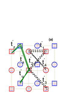
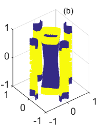
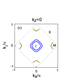
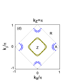
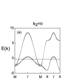
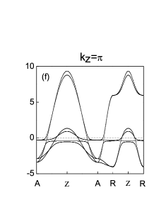
Figure 1: (Color online) (a) Schematic illustration of hopping energy parameters of the three dimensional tight-bind model $-t_{\mathrm{ij}}c^{{\dagger}}_{\mathrm{i}}c_{\mathrm{j}}$ [$\mathrm{i}$ denotes all the index of the site $i$] with three Fe orbitals $d_{xz}$, $d_{yz}$ and $d_{z^{2}}$ in real space. The red symbols denote the sites in one Fe layer, and the blue symbols denote those in the adjacent Fe layer. The two inequivalent Fe atoms are denoted by circles and squares. Hopping in the same layer is linked by black dashed lines, while hopping between adjacent layers is linked by solid olive ones. (b) The three-dimensional Fermi surface topologies of BaFe₂(As_1-xP_x)₂ for $x=0.18$. The label of the space axes is $k_{i=x,y,z}/\pi$. For the three dimensional Fermi surface topologies, blue (yellow) points represent plus (minus) signs of superconducting order in the band space, which appears after introducing the interactions. The contour plot of the three-dimensional Fermi surface structure (c) for $k_{z}=0$ and (d) for $k_{z}=\pi$. The dashed lines denote the first Brillouin zone with two Fe atoms per unit cell. The band structure is plotted along the high symmetric $\mathbf{k}$-points for (e) $k_{z}=0$ and (f) $k_{z}=\pi$. The gray dashed line denotes the Fermi level.

According to the fact of experimental measurements Shishido ; Hashimoto , we extend the two-dimensional phenomenological model with two orbitals zhang to a three-dimensional model with three orbitals to study the superconducting electronic properties in isovalent-doped BaFe₂(As_1-xP_x)₂. The previous two-dimensional model considered the effect of asymmetric arsenic atoms is appropriate to describe the experimental observations in ARPES and scanning tunnel microscope for the 122 family huang4 ; huang3 ; jian1 ; yi4 . The calculated superfluid density is in qualitative agreement with the direct experimental measurement in films of Fe pnictide superconductors at low temperatures Jyong . In the extended model, a unit cell contains two Fe atoms, and each Fe involves three orbitals $d_{xz}$, $d_{yz}$ and $d_{z^{2}}$. As arsenic is gradually substituted by phosphorus, the $d_{z^{2}}$ orbital of Fe will be driven close to the Fermi level Yueh ; liwei , resulting in an enhancement of interlayer hybridization between two interlayer Fe orbitals.

In Fig. 1(a), we show a schematic illustration of tight-binding model Hamiltonian in real space, where $t^{\prime}_{1-4}$ are hopping energies within each Fe layer between $d_{xz}$ and $d_{yz}$ orbitals. Here, it should be noted that $t^{\prime}_{2}$ is different from $t^{\prime}_{3}$ since asymmetric arsenic ions is above and below the Fe layer alternatively zhang . $t^{\prime}_{z,s,u}$ are the interlayer hopping energies between two adjacent Fe layers. $t^{\prime}_{z}$ denotes the nearest-neighbor hopping energy along the $z$ axis between $d_{z^{2}}$ and $d_{xz}$($d_{yz}$) orbitals, which can be regarded as two-step hopping processes $c^{{\dagger}}_{i+z}A_{i+z/2}A^{{\dagger}}_{i+z/2}c_{i}+H.c.$ mediated by arsenic (denoted by A) in the crystal structure environment of BaFe₂(As_1-xP_x)₂. Under the $C_{2}$ rotation at site $i$, $c^{{\dagger}}_{i+z,\beta\sigma}A_{i+z/2}\longrightarrow-c^{{\dagger}}_{i-z,\beta}A_{i-z/2\sigma}$, the combination of $c^{{\dagger}}_{i+z,\beta\sigma}A_{i+z/2}-c^{{\dagger}}_{i-z,\beta\sigma}A_{i-z/2}$ will replace the hopping term $c^{{\dagger}}_{i+z}A_{i+z/2}$ Yueh ; wen , and thus the two step hopping processes become $-4t_{z}\sin^{2}{k_{z}}$ after omitting the creation and annihilation operators of arsenic. $t^{\prime}_{s}$($t^{\prime}_{u}$) is the hopping energy along $\hat{x}\pm\hat{y}\pm\hat{z}$ between the same (different) $d_{xz},d_{yz}$ orbitals in two adjacent Fe layers. Using the Fourier transformation, the tight-binding model Hamiltonian in momentum space can be rewritten as:

$$H_{t,k}\!\! = \!\!\sum_{k\nu\sigma R}a_{1}c^{{\dagger}}_{A\nu\sigma k}c_{A\nu\sigma k}+a_{2}c^{{\dagger}}_{B\nu\sigma k}c_{B\nu\sigma k}+a_{3}c^{{\dagger}}_{R\nu\sigma k}c_{R\bar{\nu}\sigma k}$$ (1)

$$+ a_{4}c^{{\dagger}}_{A\nu\sigma k}c_{B\nu\sigma k}+a_{5}c^{{\dagger}}_{R\nu\sigma k}c_{R\beta\sigma k}+H.c.,$$

where $R=A,B$ denotes two inequivalent sites of Fe atoms, $\nu$ denotes the orbitals of $d_{xz},d_{yz}$, $\beta$ is the $d_{z^{2}}$ orbital, and $\sigma$ is the spin. Comparing hopping terms in k space with the hopping parameters in real space, we obtain the coefficients in model Hamiltonian (1) as follows

$$a_{1} = -2t_{2}\cos{(k_{x}+k_{y})}-2t_{3}\cos{(k_{x}-k_{y})}$$

$$-2t_{s}(1-\cos{k_{z}})(\cos{(k_{x}+k_{y})}+\cos{(k_{x}-k_{y})}),$$

$$a_{2} = -2t_{3}\cos{(k_{x}-k_{y})}-2t_{2}\cos{(k_{x}+k_{y}})$$

$$-2t_{s}(1-\cos{k_{z}})(\cos{(k_{x}+k_{y})}+\cos{(k_{x}-k_{y})}),$$

$$a_{3} = -2t_{4}(\cos{(k_{x}+k_{y})}+\cos{(k_{x}-k_{y})})$$

$$-2t_{u}(1-\cos{k_{z}})(\cos{(k_{x}+k_{y})}+\cos{(k_{x}-k_{y})}),$$

$$a_{4} = -2t_{1}(\cos{k_{x}}+\cos{k_{y}}),$$

$$a_{5} = -2t_{z}(1-\cos{k_{z}}),$$

with $t_{2,3}=t^{\prime}_{2,3}-t_{s},t_{4}=t^{\prime}_{4}-t_{u}$, $t_{z,s,u}=-2t^{\prime}_{z,s,u}$, $t_{1}=t^{\prime}_{1}$ as shown in Fig. 1(a).

Diagonalizing the model Hamiltonian (1), we plot the three-dimensional Fermi surface topology as shown in Fig. 1(b). There are two quasi cylindrical shells around the $\Gamma$ point and two quasi cylindrical shells around the $M$ point. Figure  1(b) also shows the variation of the three dimensional Fermi surface along the $z$ direction, which is quite different from that in LaOFeAs superconductors IIMazin . For more detail, we depict the contour plots of the three dimensional Fermi surface for $k_{z}=0$ and $k_{z}=\pi$ in Figs. 1(c) and (d), respectively. The two Fermi surface circles around the $\Gamma$ point are enlarged; in particular, the inner circle grows significantly with increasing $k_{z}$ along the $z$ direction, while the variation of cylindrical shells around the $M$ points is insignificant. Those low-energy electronic behaviors are in good agreement with previous ARPES measurements Shishido ; Hashimoto . In addition, the corresponding electronic band structures $E(k_{x},k_{y},k_{z})$ are plotted for $k_{z}=0$ and $k_{z}=\pi$ respectively, in Figs. 1(e) and (f) along the high-symmetry $\mathbf{k}$-points. For the tight-binding model, there are six bands, where the two bands of $d_{z^{2}}$ orbital are degenerate and dispersive below the Fermi level for $k_{z}=0$ shown in Fig. 1(e). However, for a finite $k_{z}$, the two degenerate flat bands will be split and become much more dispersive, which can be seen clearly in Fig. 1(f).

Taking the strong Coulomb interactions between itinerant electrons in Fe three-dimensional ($3D$) orbitals into account, we write the interaction Hamiltonian on a mean-field level as $H_{int}=H^{xy}_{int}+H^{z}_{int}$, which is expressed as zhou ; ygao ; amo :

$$H^{xy}_{int} = U\!\!\sum_{i\sigma\nu}\!\langle n_{{i}\nu\bar{\sigma}}\rangle n_{{i}\nu\sigma}+(U-3J_{H})\sum_{i\nu\sigma}\langle n_{i\nu\sigma}\rangle n_{i\nu\sigma}$$ (2)

$$+(U-2J_{H})\sum_{i\nu\sigma}\langle n_{i\nu\bar{\sigma}}\rangle n_{i\nu\sigma}-\sum_{i\nu\sigma}\mu n_{i\nu\sigma},$$

$$\hat{H}^{z}_{int} = \sum_{i\sigma}U_{z}\langle n_{i\beta\sigma}\rangle n_{i\beta\bar{\sigma}}-\mu_{1}n_{i\beta\sigma},$$ (3)

where the parameter $J_{H}$ denotes the Hund’s coupling, and $U$ and $U_{z}$ describe on-site Coulomb interaction on the $d_{xz}$($d_{yz}$) and $d_{z^{2}}$ orbitals, respectively. Since the $d_{z^{2}}$ orbital is far below the Fermi level liwei in the parent compound BaFe₂As₂, without loss of generality, we set $\mu_{1}=\mu+1.36$ and search $\mu$ self-consistently to fix the total electron number as a constant (4 electron/per Fe atom) throughout all calculations. All interactions and hopping parameters, such as $t_{2}$, $t_{3}$, and $t_{z}$, are doping dependent with fixed relations of $t_{s}=-t_{z}$, $t_{u}=0.2t_{z}$, and $t_{4}=0.04$. The wave vector $\bf{k}$ is restricted in the magnetic Brillouin zone, ascribed to the system displaying a spin-density wave order. In addition, the local electron density is expressed as $n_{i\nu\sigma}=\frac{1}{4}\langle n_{i}\rangle+\sigma M_{i}$, and the magnetic order is described as $M=\frac{1}{2}\sum_{\nu}(n_{A\nu\uparrow}-n_{A\nu\downarrow})=\frac{1}{2N_{s}}\sum_{\nu,\bf{k}}\sigma c^{{\dagger}}_{A\nu\sigma\bf{k}}c_{A\nu\sigma\bf{\bf{k+Q}}}$. Here $N_{s}$ is the number of unit cells, and $Q=(0,\pm\pi)$ or $(\pm\pi,0)$ is the wave vector of spin-density wave order Rotter .

Furthermore, we consider the intralayer and interlayer superconducting pairings between the same $d_{xz}$ and $d_{yz}$ orbitals as $H_{\Delta}=\sum_{R\nu\tau\tau^{\prime}}\Delta^{R\nu}_{i,i+\tau}c^{{\dagger}}_{i\nu\uparrow}c^{{\dagger}}_{i+\tau,\nu\downarrow}+h.c.$, where $\tau=x\pm y$ and $\tau^{\prime}=x\pm y\pm z$. In momentum space, the superconducting Hamiltonian reads $H_{\Delta,k}=\sum_{R\nu\bf{k}}(\Delta_{R\nu\bf{k}}c^{{\dagger}}_{R\nu\bf{k}\uparrow}c^{{\dagger}}_{R\nu-\bf{k}\downarrow}+h.c.)$, with

$$\Delta_{R\nu\bf{k}}=2\sum_{\tau}\cos{\bf{k}}_{\tau}\Delta^{R\nu}_{i,i+\tau}+2\sum_{\tau^{\prime}}\cos{\bf{k}}_{\tau^{\prime}}\Delta^{R\nu}_{i,i+\tau^{\prime}}$$

$$=4\cos{k_{x}}\cos{k_{y}}(\Delta^{s}_{xy}+2\Delta_{z}\cos{k_{z}})-4\Delta^{d}_{xy}\sin{k_{x}}\sin{k_{y}},$$ (4)

where the self-consistent pairing order parameter $\Delta^{R\nu}_{i,i+\tau}=\frac{V_{\tau}}{2}\langle c^{R}_{i\nu\uparrow}c^{R}_{i+\tau,\nu\downarrow}-c^{R}_{i\nu\downarrow}c^{R}_{i+\tau,\nu\uparrow}\rangle$ can be solved numerically. Interestingly, the value of superconducting pairing order within a Fe layer can be expressed as a linear combination of $d$-wave and $s$-wave pairing orders defined by $\Delta^{s,d}_{xy}=0.5(\Delta^{R\nu}_{i,i+\hat{x}+\hat{y}}\pm\Delta^{R\nu}_{i,i+\hat{x}-\hat{y}})$, because the superconducting pairing order on $\hat{x}+\hat{y}$-orientated links is different from that on $\hat{x}-\hat{y}$-orientated ones. The interlayer pairing order is denoted $\Delta_{z}$ hereafter for short, the paring potential $V_{xy,z}=1.6$ for both intra- and interlayer superconducting pairing order. Here, it should be noted that when the pairing order parameter $\Delta_{z}$ approaches zero, the three-dimensional superconductivity will evolve into an exact two-dimensional superconducting system, and the pairing order $\Delta_{R\nu\bf{k}}$ has $s_{\pm}$ symmetry with the nodal lines located at around $k_{x}=\pm\pi/2$ and $k_{y}=\pm\pi/2$. When the pairing order parameter $\Delta_{z}$ is increased to a finite value, such as $|\frac{-\Delta^{s}_{xy}}{2\Delta_{z}}|\leq 1$, some extra nodal points will penetrate into the hole pockets at around the $\Gamma$ point.

In the numerical calculation, we set the distance between the nearest-neighbor Fe atoms and the hopping integral $t_{1}$ as the length and energy units, respectively. By self-consistently diagonalizing the $24\times 24$ total Hamiltonian in momentum space, $H^{0}_{tot}(k)=H_{t,k}+H_{\Delta,k}+H_{int,k}=\sum_{n}E_{n}\gamma^{{\dagger}}_{n}\gamma_{n}$, we obtain the eigenvalues and the corresponding eigenstates of the system, which can be used for further calculating the physical quantities, such as superfluid density and the local DOS. The unit cell is $128\times 128\times 128$ for the self-consistent calculation and $384\times 384\times 384$ for the calculations of superfluid density and band structure, as well as DOS.

III Phase diagram and London penetration depth

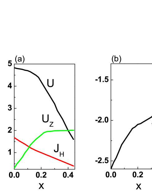
Figure 2: (color online) Doping dependent (a) Coulomb interactions including U, $J_{H}$ and $U_{z}$, hopping energy parameters (b) $t_{3}$, and (c) $t_{2}$ and $t_{z}$.

Figure 2 shows the doping dependent parameters used for the detailed calculations, including all hopping energies and interactions, $t_{2},t_{3},t_{z},U,U_{z},J_{H}$ smoothly varied under various doping concentrations. The variation of these parameters is constructed only to fit the experimental observations YZhang ; Shishido ; Hashimoto . The numerically self-consistently calculated phase diagram is shown in Fig. 3(a), which is in quit good agreement with previous experimental observations Hashimoto ; yna ; ding . The parent compound BaFe₂As₂ with antiferromagnetic order will be suppressed monotonously with increasing the doping concentration $x$. When the doping is increased beyond $x=0.08$, the superconductivity emerges, as evidenced by the appearance of the intralayer and interlayer superconducting pairing order parameters $\Delta^{s,d}_{xy}$ and $\Delta_{z}$, and then the system enters the region where magnetism and superconductivity coexist until the doping concentrations reaching $x=0.3$. If we further increase the doping concentrations, the magnetism is disappeared, and the system becomes pure superconductivity. In Fig. 3(a), we also notice that both $\Delta^{s}_{xy}$ and $\Delta_{z}$ versus dopings $x$ display a clear dome-shaped superconductivity, and the values of $\Delta^{s}_{xy}$ and $\Delta_{z}$ reach their maximum at the point of the disappearance of magnetic order. The absolute value of $|\Delta^{d}_{xy}|$ for the two different Fe sublattices is also shown in Fig. 3(a).

Next, we turn to discussing the behaviors of superfluid density based on the linear response approach. Assuming that, in the presence of a slowly varying vector potential along the $x$ direction $A_{x}(r,t)=A(q,\omega)e^{\mathrm{i}\bf{q}\cdot r_{i}-\mathrm{i}\omega t}$, all self-consistent mean-field calculations are unchanged in the framework of the linear response theory, only hopping energy terms should be modified by a Peierls phase factor, $c^{{\dagger}}_{i\sigma}c_{j\sigma}\rightarrow c^{{\dagger}}_{i\sigma}c_{j\sigma}\exp{\mathrm{i}\frac{e}{\hbar c}\int^{r_{i}}_{r_{j}}\textbf{A}(\textbf{r},t)\cdot\mathrm{d}\textbf{r}}$. Then expanding the factor to the order of $\mathbf{A}^{2}$, the perturbed Hamiltonian reads $H^{\prime}=-\sum_{i}A_{x}[eJ^{P}_{x}(r_{i})+\frac{e^{2}}{2}A_{x}K_{x}(r_{i})]$ with

$$K_{x}(r_{i}) = -\sum_{\nu\nu^{\prime}\sigma\delta}t_{i,i+\delta}x^{2}_{i,i+\delta}(c^{{\dagger}}_{i\nu\sigma}c_{i+\delta,\nu^{\prime}\sigma}+H.c.),$$ (5)

$$J^{P}_{x}(r_{i}) = -\mathrm{i}\sum_{\nu\nu^{\prime}\sigma\delta}t_{i,i+\delta}x_{i,i+\delta}(c^{{\dagger}}_{i\nu\sigma}c_{i+\delta,\nu^{\prime}\sigma}-H.c.),$$ (6)

where $\delta=x,x\pm y,x\pm y\pm z$. The total current density $J^{Q}_{x}(r_{i},t)=-\frac{\delta H^{\prime}}{\delta A_{x}(r_{i},t)}$ induced by an external magnetic field is the summation of the diamagnetic part $K_{x}$ and the paramagnetic part $J^{p}_{x}$. The calculations of $K_{x}$ are restricted to the zeroth order of $A_{x}(r_{i})$ and that of $J^{P}_{x}(r_{i})$ is restricted to the first order of $A_{x}(r_{i})$, $\langle J^{P}_{x}(r_{i})\rangle=-\frac{eA_{x}(r,t)}{N_{s}}\Pi(\bf{q},\omega)$, where $\Pi(\textbf{q},\omega)$ is obtained from the analytic continuation of the current-current correlation $\Pi(\textbf{q},\mathrm{i}\omega)=\int^{\beta}_{0}d\tau e^{\mathrm{i}\omega\tau}\Pi({\bf{q}},\tau)$ in the Matsubara formalism. Here $\Pi(\textbf{q},\tau)=-\langle T_{\tau}J^{P}_{x}(\textbf{q},\tau)J^{P}_{x}(-\textbf{q},0)\rangle_{0}$, $J^{P}_{x}(\textbf{q},\tau)\,=e^{\tau H_{0}}J^{P}_{x}(\textbf{q})e^{-\tau H_{0}}$, $J^{P}_{x}(\textbf{q})=\sum_{i}e^{-\mathrm{i}\textbf{q}\cdot\textbf{r}_{i}}J^{P}_{x}(r_{i})$, and $T_{\tau}$ is the imaginary time ordering operator. In the quasi-particle basis, the paramagnetic current can be expressed as the summation of components $J^{P}_{x}({\bf{q}})=\sum_{m_{1}m_{2}}J^{P}_{m_{1}m_{2}}$ with $J^{P}_{m_{1}m_{2}}=\gamma^{{\dagger}\bf{k}}_{m1}\gamma^{\bf{k+q}}_{m2}\Gamma^{\bf{k,k+q}}_{m_{1}m_{2}}$. After some tedious but straightforward algebraic derivations, the concrete expression of $\Gamma$ is derived. Using the equation of motion of Green’s function, we obtain huang2

$$\Pi(\textbf{q},\mathrm{i}\omega)\!\!=\!\!\!\!\!\sum_{{\bf{k}}m_{1}m_{2}\sigma}\!\!\frac{\Gamma_{m_{1}m_{2}}^{\bf{k},\bf{k+q}}\Gamma_{m_{2}m_{1}}^{\bf{k+q},\bf{k}}[f(E_{{\bf{k}},m_{1}})-f(E_{{\bf{k+q}},m_{2}})]}{\mathrm{i}\omega+(E_{{\bf{k}},m_{1}}-E_{{\bf{k+q}},m_{2}})},$$ (7)

where $f$ is the Fermi-Dirac distribution function. Thus, the superfluid density weight measured by the ratio of the superfluid density to the mass is proportional to $\Pi(\bf{q},\omega)$ in the limit of zero frequency $\omega$ and momentum $\bf{q}$ huang2 ; tdas ; djs ; fla2 and is expressed as

$$\frac{\rho_{s}}{m^{\ast}}=-\langle J^{Q}_{x}(r_{i},t)\rangle/e^{2}A_{x}(r_{i})$$ (8)

$$= \frac{1}{N_{s}}\Pi(q_{x}=0,q_{y}\rightarrow 0,q_{z}\rightarrow 0,\omega=0)-\langle K_{x}\rangle_{0}.$$

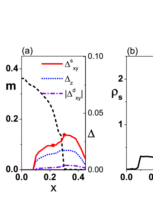
Figure 3: (Color online) (a) Doping-dependent magnetic order $m$, intralayer superconducting orders $\Delta^{s,d}_{xy}$ and interlayer superconducting order $\Delta_{z}$ for BaFe₂(As_1-xP_x)₂. (b) Superfluid density $\rho_{s}$ versus doping level $x$. (c) Square of the penetration depth $\lambda^{2}$ versus $x$.

Fig. 3(b) shows the superfluid density $\rho_{s}$ as a function of doping concentration $x$ across the whole phase diagram in Fig. 3(a) at zero temperature. At underdoped concentration $x$ around the parent compound system, the superfluid density $\rho_{s}$ is zero as expected from our intuitive knowledge that the system does not have superconducting order. As the doping concentration $x$ increases, the superconductivity emerges, accompanied by the appearance of a finite value of $\rho_{s}$. If the doping concentration $x$ is further increased, $\rho_{s}$ changes to decrease its value slowly until $x=0.22$, and then $\rho_{s}$ further goes upward with a steep slope, displaying a sharp peak at $x=0.3$ with the value of superfluid density being $8$ times larger than that at $x=0.22$. Reaching the maximal value of superfluid density $\rho_{s}$ at $x=0.3$ corresponds to the point of the disappearance of magnetic order in Fig. 3(a), denoted by the red dot in the curve of $\Delta^{s}_{xy}$. Eventually, the superfluid density $\rho_{s}$ decreases sharply and then tends to saturates to a finite value upon further increasing the doping concentration $x$.

In addition, a fundamental property of the superconducting state is the London penetration depth $\lambda$, parametrizing the ability of a superconductor to screen an applied magnetic field, which not only can be evaluated straightforwardly from the superfluid density $\rho_{s}$ but also can be measured in experiments yla . In general, $\rho_{s}$ is described as the phase rigidity of a superconductor, and it may vanish before the superconducting energy gap diminished as increasing temperature. In Fig. 3(c), we plot the square of London penetration depth $\lambda^{2}$ as a function of doping concentration $x$. It is important to point out that the value of London penetration depth $\lambda^{2}$ displays a sharp peak at $x=0.22$ which corresponds to the minimal value of $\rho_{s}$ and corresponds to the red square in the curve of $\Delta^{s}_{xy}$ in Fig. 3(a), and then it decreases sharply. Eventually, $\lambda^{2}$ becomes rather flat in the pure superconducting region. Compared with the experimental results Hashimoto , where the magnetic phase boundary corresponds to the sharp peak of $\lambda^{2}$, our numerical results show that the sharp peak penetration depth appears before the vanishing of magnetic order. Such anomalous peak in London penetration depth has never been observed experimentally in other iron-based superconductors, and it leads to a conjecture of the presence of QCP in BaFe₂(As_1-xP_x)₂.

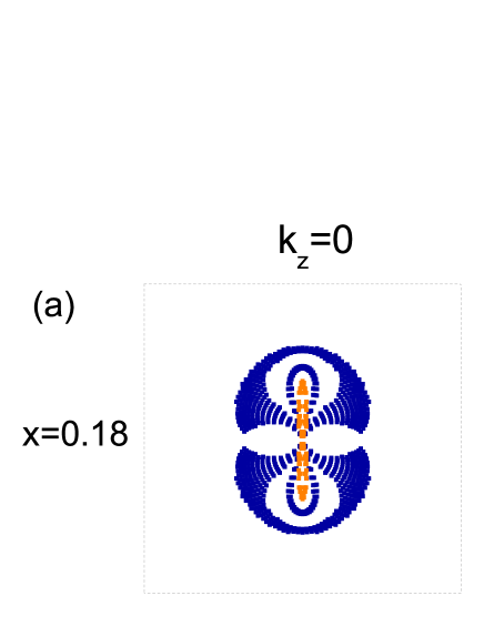
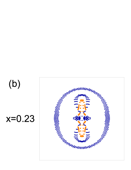
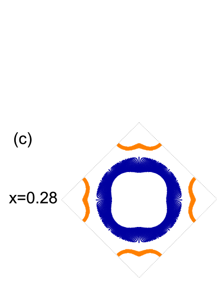
Figure 4: (Color online) Superconducting gap structure of the band space for different doping concentrations $x=0.18,0.23,0.28$ near the Fermi surface. From left to right the plots correspond to $k_{z}=0,\pi/2,\pi$, respectively. The inset of panel (c) is an enlargement of the $z$ point. The gray lines are the corresponding first Brillouin zone.

The superconducting gap structure in the band representation $\tilde{\Delta}_{k}$ is derived from the $6\times 6$ matrix Hamiltonian $H_{\Delta,k}$ of $\Delta_{k}$ (short hand for $\Delta_{R\nu k}$) in the orbital space as $[\tilde{H}_{\Delta,k}]=[W]^{{\dagger}}[H_{\Delta,k}][W]^{*}$ when magnetic order is absent, with $[W]$ being the transformation matrix diagonalizing the $6\times 6$ tight-binding Hamiltonian $H_{t,k}$, and the corresponding $\tilde{\Delta}_{k}$ are the diagonal elements of $[\tilde{H}_{\Delta,k}]$. However, for finite magnetic order the corresponding $[W]$ is a $12\times 12$ matrix diagonalizing the Hamiltonian $H_{t,k}+H_{int,k}$ including the interaction part. Figure 4 displays the behavior of $\tilde{\Delta}_{k}$ near the Fermi surface, where the navy points correspond to positive signs of $\tilde{\Delta}_{k}$ and the orange points are for the minus signs. Figure 4 shows that the gap structure in $x=0.23$ has a finite value near the Fermi surface at all $k_{z}$, which is quite different from that in the $x=0.18$ case where the node points exist. For a given doping level, a larger $k_{z}$ corresponds to a smaller magnitude of superconducting gap. It is important to point out that along the line of $k_{z}$, the superconducting gap will change signs from $0.5\pi$ to $\pi$ when we do not consider the effect of magnetic order, which can be seen clearly in Fig. 4(c), where we set the magnetic order to zero. Therefore, we expect that in the region with the sudden drop in penetration depth the corresponding $\tilde{\Delta}_{k}$ will change its structure.

IV DOS and Fermi surface topologies

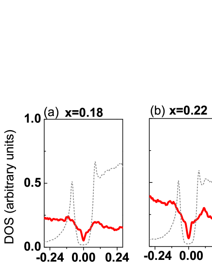
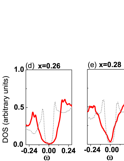
Figure 5: (Color online) (a)-(f) For $V_{z}=1.6$, DOS as a function of energy at various doping concentrations $x=0.18,0.22,0.24,0.26,0.28,0.38$ are shown by the red lines, where the gray dashed lines represent the corresponding DOS for $V_{z}=0$.

To clarify the nature of the emergence of an anomalous sharp peak in the penetration depth, we calculate the DOS for various doping concentrations $x$ at zero temperature, as shown in Fig. 5. When the doping concentration is located in the region of $x\leq 0.22$, the calculated DOS displays a “V”-shaped structure with finite value at the Fermi level, implying the presence of nodal points in the superconducting energy gap. As the doping concentration $x$ increases, the “V”-shaped DOS changes into a “U”-shaped structure at $x=0.24,0.26$ with a diminished DOS at the Fermi level; the plot for $x=0.23$ is similar to that for $x=0.24$, which we do not show here. When the doping concentration is increased beyond $0.28$, the tip at zero energy reappears [see Fig. 5(e)]. Fig. 5(f) shows a narrow “V”-shaped DOS feature in a pure superconducting region, suggesting the system is a nodal superconductor, which is in agreement with the previous ARPES measurement YZhang . Therefore, comparing Fig. 5 with Fig. 3(c) we find that the phase transition of the changing pairing order parameter from nodeless to a nodal structure is responsible for the appearance of the sharp peak in the experimental measurement of the London penetration depth.

To further understand the nature of the emergence of the anomalous sharp peak in the London penetration depth, we also plot the DOS for $\Delta_{z}=0$, a two-dimensional limited case, shown by the gray dashed lines in Fig. 5, where the interlayer interaction $V_{z}=0$ is set to zero and the other interaction parameters remain the same as in Fig. 2. For this $3D$ interaction and two-dimensional superconducting order case, the system displays a “U”-shaped DOS for all doping concentrations from $x=0.18$ to $x=0.28$.

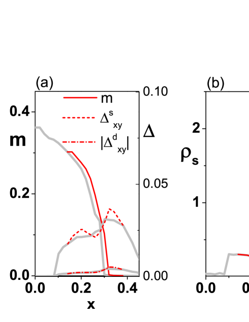
Figure 6: (Color online) In the doping region of [0.14,0.36], the red curves are doping-dependent physical quantities for the $\Delta_{z}=0$ case. (a) Magnetic order $m$ and superconducting orders $\Delta^{s,d}_{xy}$, (b) superfluid density $\rho_{s}$, and (c) the square of the penetration depth as a function of doping. The gray lines are the corresponding curves of $V_{z}=1.6$ in Fig.3.

In the case where $\Delta_{z}$ is absent, the nodal-to-nodeless transition no longer exists since all the DOS are “U”-shaped features. Although the resulting $\rho_{s}$ and $\lambda^{2}$ still have a sharp peak as that in $V_{z}=1.6$ case, which can be seen clearly in Fig. 6(b) and Fig. 6(c), a remarkable dip in the phase diagram of $\Delta^{s}_{xy}$ versus doping appears, which is ascribed to the presence of three-dimensional interaction. Figure 6(a) shows that $\Delta^{s}_{xy}$ drops to a minimum value suddenly at $x=0.24$, destroying the dome-shaped superconductivity and leading to an unphysical anomalous penetration depth. A minimum pairing order corresponding to a maximal penetration depth is a reasonable result when there is no other phase transition. Furthermore, for two-dimensional dome-shaped iron-based superconductivity huang2 , the penetration depth does not show the sharp peak. Therefore, the experimental observation of a sharp peak in penetration depth having dome-shaped superconductivity stems from three-dimensional electron interactions accompanied by a transition from nodal to nodeless pairing.

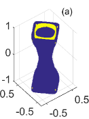
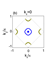
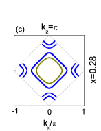
Figure 7: (Color online) (a) Three-dimensional plot of the two cylindrical shells around the $\Gamma$ point for dopant concentration of $x=0.28$. (b) and (c) are the contour plots of the Fermi surface at $k_{z}=0$ and $k_{z}=\pi$, respectively. Blue points denote the plus signs of the corresponding superconducting pairing, and dark yellow points are for the minus signs.

In addition to analyzing the numerical data for superconducting pairing order parameters, we find a nodal circle in the inner hole pocket around the $\Gamma$ point in the vicinity of $k_{z}=0.86\pi$ for $x=0.28$, and four nodal points in the outer hole pocket, which is shown in Fig. 7(a) with the boundaries of the two colors denoting the nodal points on the $3D$ Fermi surface topologies. For $k_{z}>0.86\pi$, the superconducting pairing in the inner hole pocket changes sign, while the points on the outer pocket remain the same color as that of small $k_{z}$, which is quite different from $x=0.18$ shown in Fig. 1(b). In order to unambiguously display the inner shape of Fermi surface topologies, Figs. 7(b) and (c) depict the contour plot of Fermi surface for $k_{z}=0$ and for $k_{z}=\pi$ at $x=0.28$, respectively. For $k_{z}=\pi$ the superconducting gap has different signs on the outer and inner hole pockets, which is different from $x=0.18$ but consistent with the inset of Fig.4. It is worth pointing out that the small inner circle of the hole pocket around the $\Gamma$ point in the Brillouin zone is easily immersed if the doping concentration is increased further. The larger $k_{z}$ has a larger Fermi surface circle; however the magnitude of the corresponding superconducting pairing is small as shown in Fig. 4. Those calculations further solidify the nature of nodeless-to-nodal transition in doped BaFe₂(As_1-xP_x)₂, leading to the appearance of an anomalous sharp peak in the London penetration depth.

V summary

In this paper, we constructed a three-dimensional tight-binding lattice model based on the facts from the penetration depth and the ARPES experimental measurements. Taking the interlayer Coulomb interactions into account, the superconducting phase diagram and an anomalous sharp peak in the London penetration depth were evaluated, and are entirely in good agreement with experimental observations. By verifying the DOS and the pairing order parameters as well as the Fermi surface topologies at various doping concentrations, we find that the QCP originates from the nature of three-dimensional interactions, leading to a phase transition from a nodeless to a nodal pairing symmetry. This finding provides significant insight into the understanding of the nature of the QCP that emerged in the London penetration depth experiment in the isovalent doped superconductor BaFe₂(As_1-xP_x)₂.

VI acknowledgments

This work was supported by the National Key Research and Development Programs of China (Grant Nos. 2017YFA0304204 and 2016YFA0300504), Nat Basic Research Program of China (Grant No. 2914CB921203), the National Natural Science Foundation of China (Grant Nos. 11625416, 11474064, 11674278, 11927807 and 11774218),Shanghai Municipal Government under the Grant No. 19XD1400700, the Natural Science Foundation of Shanghai of China (Grant Nos. 18JC1420402 and 19ZR1402600), and the Natural Science Foundation from Jiangsu Province of China (Grant No. BK20160094). W. L. also acknowledges the start-up funding from Fudan University.

References

- (1) Y. Kamihara, T. Watanabe, M. Hirano, and H. Hosono, J. Am. Chem. Soc. 130, 3296 (2008).
- (2) H. Ding, P. Richard, K. Nakayama, K. Sugawara, T. Arakane, Y. Sekiba, A. Takayama, S. Souma, T. Sato, T. Takahashi, Z. Wang, X. Dai, Z. Fang, G. F. Chen, J. L. Luo, and N. L. Wan, Europhys. Lett. 83, 47001 (2008).
- (3) G. R. Stewart, Rev. Mod. Phys. 83, 1589 (2011).
- (4) A. Damascelli, Z. Hussain, and Z.-X. Shen, Rev. Mod. Phys. 75, 473 (2003).
- (5) C. C. Tsuei and J. R. Kirtley, Rev. Mod. Phys. 72, 969 (2000).
- (6) M. Rotter, M. Tegel, D. Johrendt, I. Schellenberg, W. Hermes, and R. Pöttgen, Phys. Rev. B 78, 020503(R) (2008).
- (7) H. Shishido, A. F. Bangura, A. I. Coldea, S. Tonegawa, K. Hashimoto, S. Kasahara, P. M. C. Rourke, H. Ikeda, T. Terashima, R. Settai, Y. Önuki, D. Vignolles, C. Proust, B. Vignolle, A. McCollam, Y. Matsuda, T. Shibauchi, and A. Carrington, Phys. Rev. Lett. 104, 057008 (2010).
- (8) S. Kasahara, T. Shibauchi, K. Hashimoto, K. Ikada, S. Tonegawa, R. Okazaki, H. Shishido, H. Ikeda, H. Takeya, K. Hirata, T. Terashima, and Y. Matsuda, Phys. Rev. B 81, 184519 (2010).
- (9) H. Suzuki, T. Kobayashi, S. Miyasaka, T. Yoshida, K. Okazaki, L. C. C. Ambolode, S. Ideta, M. Yi, M. Hashimoto, D. H. Lu, Z.-X. Shen, K. Ono, H. Kumigashira, S. Tajima, and A. Fujimori, Phys. Rev. B 89, 184513 (2014).
- (10) M. Dzero, M. Khodas, A. D. Klironomos, M. G. Vavilov, and A. Levchenko, Phys. Rev. B 92, 144501 (2015).
- (11) Y. Murakami, P. Werner, N. Tsuji, and H. Aoki, Phys. Rev. Lett. 113, 266404 (2014).
- (12) K. Hashimoto, K. Cho, T. Shibauchi, S. Kasahara, Y. Mizukami, R. Katsumata, Y. Tsuruhara, T. Terashima, H. Ikeda, M. A. Tanatar, H. Kitano, N. Salovich, R. W. Giannetta, P. Walmsley, A. Carrington, R. Prozorov, and Y. Matsuda, Science 336, 1554 (2012).
- (13) Y. Nakai, T. Iye, S. Kitagawa, K. Ishida, H. Ikeda, S. Kasahara, H. Shishido, T. Shibauchi, Y. Matsuda, and T. Terashima, Phys. Rev. Lett 105, 107003 (2010).
- (14) R. M. Fernandes, S. Maiti, P. Wölfle, and A. V. Chubukov, Phys. Rev. Lett. 111, 057001 (2013).
- (15) Z. Diao, D. Campanini, L. Fang, W.-K. Kwok, U. Welp, and A. Rydh, Phys. Rev. B 93, 014509 (2016).
- (16) M. P. Smylie, M. Leroux, V. Mishra, L. Fang, and K. M. Taddei, O. Chmaissem, H. Claus, A. Kayani, A. Snezhko, U. Welp, W. K. Kwok, Phys. Rev. B 93, 115119 (2016).
- (17) Debanjan Chowdhury, Brian Swingle, Erez Berg, and Subir Sachdev, Phys. Rev. Lett. 111, 157004, (2013).
- (18) J.-H. Dai, Q. M. Si, J.-X Zhu and E. Abrahams, Proc. Natl. Acad. Sci. 106, 4118, (2009).
- (19) M. A. Tanatar, K. Hashimoto, S. Kasahara, T. Shibauchi, Y. Matsuda, and R. Prozorov, Phys. Rev. B 87, 104506 (2013).
- (20) A. Levchenko, M. G. Vavilov, M. Khodas, and A. V. Chubukov, Phys. Rev. Lett. 110, 177003 (2013).
- (21) Y. Lamhot, A. Yagil, N. Shapira, S. Kasahara, T. Watashige, T. Shibauchi, Y. Matsuda, and O. M. Auslaender, Phys. Rev. B 91, 060504(R) (2015).
- (22) M. Dzero and A. Levchenko,Phys. Rev. B 98, 054501 (2018).
- (23) K. R. Joshi, N. M. Nusran, M. A. Tanatar, K. Cho, S. L. Bud ko, P. C. Canfield, R. M. Fernandes, A. Levchenko, R. Prozorov, arXiv:1903.00053v1 (2019).
- (24) H. X. Huang, Y. Gao, J.-X. Zhu, and C. S. Ting, Phys. Rev. Lett. 109, 187007 (2012).
- (25) T. Nomoto and H. Ikeda, Phys. Rev. Lett. 111, 167001 (2013).
- (26) P. Walmsley, C. Putzke, L. Malone, I. Guillamón, D. Vignolles, C. Proust, S. Badoux, A. I. Coldea, M. D.Watson, S. Kasahara, Y. Mizukami, T. Shibauchi, Y. Matsuda, and A. Carrington, Phys. Rev. Lett. 110, 257002 (2013).
- (27) D. Chowdhury, J. Orenstein, S. Sachdev, and T. Senthil, Phys. Rev. B 92, 081113 (2015).
- (28) Y. Zhang, Z. R. Ye, Q. Q. Ge, F. Chen, J. Jiang, M. Xu, B. P. Xie and D. L. Feng, Nat. Phys. 8, 371 (2012).
- (29) W. Li, J. X. Zhu, Y. Chen, and C. S. Ting, Phys. Rev. B 86, 155119 (2012).
- (30) K. Suzuki, H. Usui, and K. Kuroki, J. Phys. Soc. Jpn. 80, 013710 (2011).
- (31) D. Zhang, Phy. Rev. Lett. 103, 186402 (2009), Phy. Rev. Lett. 104, 089702 (2010).
- (32) H. Huang, Y. Gao, D. Zhang, and C. S. Ting, Phys. Rev. B 84, 134507 (2011).
- (33) H. Huang, D. Zhang, Y. Gao, W. Ren, and C. S. Ting, Phys. Rev. B 93, 064519 (2016).
- (34) Jian-Xin Zhu, Jean-Pierre Julien, Y. Dubi, and A. V. Balatsky Phys. Rev. Lett. 108 186401 (2012).
- (35) Yi Gao, Jian-Xin Zhu, C. S. Ting, and Wu-Pei Su Phys. Rev. B 84 224509 (2011).
- (36) J. Yong, S. Lee, J. Jiang, C. Bark, J. Weiss, E. Hellstrom, D. Larbalestier, C. Eom, and T. Lemberger, Phys. Rev. B 83, 104510 (2011).
- (37) Y. H. Su, C. Setty, Z. Q. Wang, and J. P. Hu, Phys. Rev. B 85, 184517(2012).
- (38) P. A. Lee and X.-G. Wen, Phys. Rev. B 78, 144517 (2008).
- (39) I. I. Mazin, D. J. Singh, M. D. Johannes, and M. H. Du, Phys. Rev. Lett. 101, 057003 (2008).
- (40) T. Zhou, D. Zhang, and C. S. Ting, Phys. Rev. B 81, 052506 (2010).
- (41) Y. Gao, H. X. Huang, C. Chen, C. S. Ting, and W.-P. Su, Phys. Rev. Lett. 106, 027004 (2011).
- (42) A. M. Oleś, G. Khaliullin, P. Horsch, and L. F. Feiner, Phys. Rev. B 72, 214431 (2005).
- (43) D. Hu, X. Lu, W. Zhang, H. Luo, S. Li, P. Wang, G. Chen, F. Han, S.R. Banjara, A. Sapkota, A. Kreyssig, A. I. Goldman, Z. Yamani, C. Niedermayer, M. Skoulatos, R. Georgii, T. Keller, P. Wang, W. Yu, and P. Dai, Phys. Rev. Lett. 114, 157002 (2015).
- (44) T. Das, J. X. Zhu, and M. J. Graf, Phys. Rev. B 84, 134510 (2011).
- (45) D. J. Scalapino, S. R. White, and S. C. Zhang, Phys. Rev. B 47, 7995 (1993).
- (46) L. Liang, T. I. Vanhala, S. Peotta, T. Siro, A. Harju, and P. Törmä, Phys. Rev. B 95, 024515 (2017).