A Case Study on Using Deep Learning for Network Intrusion Detection
Abstract
Deep Learning has been very successful in many application domains. However, its usefulness in the context of network intrusion detection has not been systematically investigated. In this paper, we report a case study on using deep learning for both supervised network intrusion detection and unsupervised network anomaly detection. We show that Deep Neural Networks (DNNs) can outperform other machine learning based intrusion detection systems, while being robust in the presence of dynamic IP addresses. We also show that Autoencoders can be effective for network anomaly detection.
Index Terms:
Network Intrusion Detection, Deep Learning, Deep Neural Network, Autoencoder, Anomaly DetectionI Introduction
As the scale of cyber attacks and volume of network data increases exponentially, organizations must continually adapt against the dynamic nature of evolving cyber threat actors. With more security tools and sensors being deployed in modern enterprise networks, the number of security events being generated continues to increase, making it more challenging to detect malicious activities. Organizations must adopt new techniques to augment human analysts in monitoring, preventing, detecting, and responding to cybersecurity events and potential attacks. Machine Learning has been deemed by many as a game changer in cyber defense. However, the usefulness of Deep Learning in the context of Network Intrusion Detection Systems (NIDSs) has not been systematically understood, despite its tremendous success in other application domains (e.g., image recognition).
I-A Our contributions
The contribution of this work is two-fold. First, we propose using a feedforward fully connected Deep Neural Network (DNN) to train a NIDS via supervised learning. We also propose using an autoencoder to detect and classify attack traffic via unsupervised learning in the absence of labeled malicious traffic. Second, we evaluate these models using two recent network intrusion detection datasets with known ground truth of malicious vs. benign traffic. We show (i) DNN outperforms other machine learning based network intrusion detection systems; (ii) DNN is robust in the presence of dynamic IP addresses assigned by the Dynamic Host Configuration Protocol (DHCP), which is important when we need to use IP addresses as features in training DNNs; and (iii) autoencoder is effective for anomaly detection.
I-B Related work
Intrusion detection can be host-based or network-based, with this paper being in the latter category. There are multiple approaches to network-based intrusion detection. The idea of anomaly detection can be traced back as early as the 19th century with origins in the statistics community [1]. The study of intrusion detection for cybersecurity is introduced in 1987 [2]. Fiore et al. [3] explored the use of a semi-supervised model for network intrusion detection, using a Discriminative Restricted Boltzmann Machine. However, their study is based on the KDD 99 dataset [4], which is outdated now [5].
In addition to the KDD 99 dataset, there are other datasets, such as: the CAIDA dataset [6], the DARPA/Lincoln Lab packet trace [7, 8], and the Lawrence Berkeley National Laboratory (LBNL) and ICSI Enterprise Tracing Project [9]. However, comparative studies of these datasets [10, 11] found that some are outdated and unreliable because they lack a diversity of traffic and volumes, some lack a variety of attacks, some are anonymized and lack valuable payload information, and some lack feature set and metadata.
The present paper focuses on using newer datasets that have recently become available to the research community. Not only do these newer datasets contain modern-day attacks, they are created in such a way as to follow established guidelines of reliable intrusion detection datasets (in terms of realism, evaluation capabilities, total capture, completeness, and malicious activity) [11]. There are a number of other studies that use these datasets for evaluation in their work. However, many evaluating the ISCX IDS 2012 dataset [11] use only a subset of the data, and vary in their ways for generating the ground truth [12, 13, 14, 15, 16]. Studies conducted with the CIC IDS 2017 dataset [11] have used other types of machine learning techniques than Deep Learning [17, 18, 19, 20, 21, 22, 23]. More recent studies have begun to use Deep Learning with the CIC IDS 2017 dataset; however, some only use a subset of the data for detecting one type of attack (e.g., port scan, DDoS) [24, 25, 26] or generate their own flows instead of using the ground truth flows [27]. The present study differs in that it evaluates both supervised and unsupervised deep learning approaches across the full spectrum of attacks, while using the entirety of the datasets as well as the ground truth provided.
Intrusion detection is an important field of cybersecurity data analytics [28, 29, 30, 31, 32, 33, 34, 35, 36], which is one pillar underlying the Cybersecurity Dynamics framework [37, 38] that aims to model and quantify cybersecurity from a holistic perspective. The other two pillars are known as first-principle modeling and analysis [39, 40, 41, 42, 43, 44, 45] and cybersecurity metrics [46, 47, 48, 49].
II Preliminaries
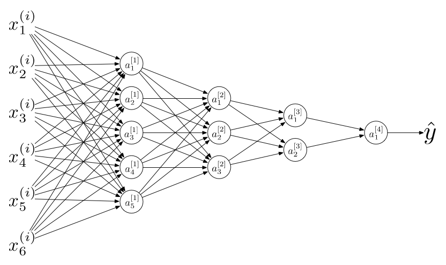
DNNs are a powerful mechanism for supervised learning. They can represent functions of increasing complexity, by inclusion of more layers and more units per layer in a neural network [50]. In the context of NIDSs, DNNs can be used to discover patterns of benign and malicious traffic hidden within large amounts of structured data. Figure 1 is an example of a standard Deep Learning representation, where nodes represent inputs, edges represent weights, superscript denotes the th training example, and superscript denotes the th layer. Our case study focuses on DNNs because they can cope with tabular data and categorical variables of high cardinality, which are exhibited by the datasets we analyze.
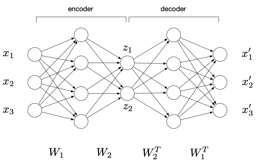
Autoencoder is another type of neural network and is trained in such a way that it aims to copy its input to its output, namely aiming to find a lower dimensional, latent space representation of the input data [50]. Unlike other popular dimensionality reduction techniques such as Principle Component Analysis (PCA), it achieves its goal in a non-linear fashion. Figure 2 shows an example standard Autoencoder, where the number of input neurons is equal to the number of output neurons. We choose Autoencoder for our case study on anomaly detection because of its usefulness given lots of normal data, and its applicability to situations where it may be difficult to explain what represents anomalous data.
III Case Study
III-A Methodology
Deep Learning excels when there is a large amount of training data [50]. This suggests that we use the newer datasets for our case study: the ISCX IDS 2012 dataset [11] has over 2.54M examples (including 2.47M benign ones and 68,910 malicious ones); the CIC IDS 2017 dataset [10] has over 2.83M examples (including 2.27M benign ones and 557,646 malicious ones). In contrast, older datasets are often small (e.g., the KDD 99 dataset [4] has only 148,517 flows, including 77,054 benign ones and 71,463 malicious ones).
We choose DNNs because they can cope with tabular data that contains categorical variables of high cardinality, which are exhibited by the two newer datasets we use. A key issue is to cope with categorical features of high cardinality [51]. The idea is to use entity embedding to map categorical features of high cardinality to low-dimensional real vectors in such a way that similar values remain close to each other [52, 53].
We choose Autoencoders because they are useful when there are lots of examples of normal data, while it may be difficult to explain what represents anomalous data [11]. Autoencoders learn a compressed representation of the input data, meaning that its output is a reconstruction of the input data in a certain form. By minimizing the error of reconstructing the normal input (i.e., benign flows), Autoencoders learn to modify the weights for reconstructing the input. When an Autoencoder encounters a malicious flow, the reconstruction error would be high (in comparison to reconstructing a normal flow).
III-B Data description
The ISCX IDS 2012 dataset [11] was created by modeling a given network environment with a testbed and then using agents to perform attacks on the testbed network. When compared with the outdated datasets [7, 8, 4], this dataset can be characterized as follows [11]: realistic network configuration because of the real testbed; realistic traffic because of the real attacks/exploits; labeled ground truth of benign and malicious traffic; total capture of communications; and diverse attack scenarios. This dataset is provided in PCAP as well as a custom XML file of network flows created with the IBM QRadar appliance; the XML flow file contains ground truth labels. Recall that a network flow is assembled from a number of IP packets and consists of source and destination IP addresses, source and destination port numbers, and protocol. Moreover, flows are often used as a unit for detecting attacks, which is our focus in the present study (another unit is IP packet). Table I provides an overview of this dataset.
| Date | # of Flows | # of Attacks | Description |
| 6/11/2012 | 474,278 | 0 | Benign network activities |
| 6/12/2012 | 133,193 | 2,086 | Brute-force against SSH |
| 6/13/2012 | 275,528 | 20,358 | Infiltrations internally |
| 6/14/2012 | 171,380 | 3,776 | HTTP DoS attacks |
| 6/15/2012 | 571,698 | 37,460 | DDoS using IRC bots |
| 6/16/2012 | 522,263 | 11 | Brute-force against SSH |
| 6/17/2012 | 397,595 | 5,219 | Brute-force against SSH |
| Total | 2,545,935 | 68,910 | 2.71% malicious |
Table II summarizes the 14 features that can be extracted from the labeled XML file of network flows.
| No. | Feature | Description | Type | Uniques |
| 1 | SrcIP | Source IP address | Categorical | 2,478 |
| 2 | DstIP | Dest. IP address | Categorical | 34,552 |
| 3 | SrcPort | Source port | Categorical | 64,482 |
| 4 | DstPort | Dest. port | Categorical | 24,238 |
| 5 | AppName | Application name | Categorical | 107 |
| 6 | Direction | Direction of flow | Categorical | 4 |
| 7 | Protocol | IP protocol | Categorical | 6 |
| 8 | Duration | Flow duration | Continuous | N/A |
| 9 | TotalSrcBytes | Total source bytes | Continuous | N/A |
| 10 | TotalDstBytes | Total dest. bytes | Continuous | N/A |
| 11 | TotalBytes | Total bytes | Continuous | N/A |
| 12 | TotalSrcPkts | Total source packets | Continuous | N/A |
| 13 | TotalDstPkts | Total dest. packets | Continuous | N/A |
| 14 | TotalPkts | Total packets | Continuous | N/A |
The CIC IDS 2017 dataset [10] improves the ISCX IDS 2012 dataset by containing, along with benign traffic, attack traffic from seven different kinds of attacks (i.e., brute-force against the SSH and Web, Heartbleed, botnet, denial of service (DoS), distributed denial of service (DDoS), cross-site scripting (XSS) and SQL injection attacks against websites, and infiltration). This dataset includes not only the raw PCAP data, but also pre-processed network flow data from the PCAP data (processed using the CICFlowMeter tool [54]). This pre-processed network flow data is provided as CSV files that can be fed into the machine learning pipeline. The pre-processed network flow data has 83 columns (e.g., duration, number of packets, number of bytes, length of packets) that can be used as features, plus one label column and one flow ID column. Since seven different kinds of attacks are contained in this dataset, we can conduct multiclass classification research. Table III shows a summary of this dataset.
| Date | # of Flows | # of Attacks | Description |
| Monday | 529,918 | 0 | Normal activities |
| Tuesday | 445,909 | 7,938 | FTP-Patator |
| 5,897 | SSH-Patator | ||
| Wednesday | 692,703 | 5,796 | DoS slowloris |
| 5,499 | DoS Slowhttptest | ||
| 231,073 | DoS Hulk | ||
| 10,293 | Dos GoldenEye | ||
| 11 | Heartbleed | ||
| Thursday AM | 170,366 | 1507 | Web - Brute Force |
| 652 | Web - XSS | ||
| 21 | Web - SQL Injection | ||
| Thursday PM | 288,602 | 36 | Infiltration |
| Friday AM | 191,033 | 1966 | Bot |
| Friday PM 1 | 286,467 | 158,930 | PortScan |
| Friday PM 2 | 225,745 | 128,027 | DDoS |
| Total | 2,830,743 | 557,646 | 19.70% malicious |
Table IV highlights some of the 74 features that were “useable” from the CIC IDS 2017 dataset, while noting that among the other 85-74=11 features, eight continuous features contain no variability or missing values and therefore are discarded, and the remaining three are FlowID, the timestamp, and the label (used for the predicted class).
| No. | Feature | Description | Type | Uniques |
| 1 | SrcIP | Source IP address | Categorical | 17,002 |
| 2 | DstIP | Dest. IP address | Categorical | 19,112 |
| 3 | SrcPort | Source port | Categorical | 64,638 |
| 4 | DstPort | Dest. port | Categorical | 53,791 |
| 5 | Protocol | IP protocol | Categorical | 3 |
| 6 | Duration | Flow duration | Continuous | N/A |
| 7 | total_fpackets | Total num. forward packets | Continuous | N/A |
| 8 | total_bpackets | Total num. backward packets | Continuous | N/A |
| 9 | total_fpktl | Total size of forward packets | Continuous | N/A |
| 10 | total_bpackets | Total size of backward packets | Continuous | N/A |
| 70 | std_active | Std. dev time flow active before idle | Continuous | N/A |
| 71 | min_idle | Min time flow idle before active | Continuous | N/A |
| 72 | mean_idle | Mean time flow idle before active | Continuous | N/A |
| 73 | max_idle | Max time flow idle before active | Continuous | N/A |
| 74 | std_idle | Std. dev time flow idle before active | Continuous | N/A |
III-C Using DNNs for network intrusion detection
III-C1 Pre-processing
We propose formatting a dataset (more specifically, network flows) in such a way that can be input into a DNN. Recall that the ISCX IDS 2012 dataset is provided in PCAP as well as a custom XML file of network flows with associated ground-truth labels (indicating malicious or benign flows). The XML file is parsed and converted to a CSV file of flows, which becomes the input into the machine learning pipeline. Recall that the CIC IDS 2017 dataset is in the form of both PCAP as well as flows characterized by 74 usable features (5 categorical and 69 statistical).
In order to make machine learning algorithms train models in the same feature space, it is a common practice to normalize or scale the continuous values among all the features. For this purpose, we use the standard min-max scaling, which is a normalization method for scaling data to [0,1] as follows: , where and are respectively the minimum and maximum value of feature .
In order to train DNNs over categorical data, we need to convert them to numerical values. For this purpose, we propose adopting the entity embedding technique [51] because it can cope with categorical features that take a large number of possible values. This is true for the datasets we analyze because there are many possible values for source IP addresses, destination IP addresses, source port numbers, and destination port numbers. In the entity embedding method, the number of embedding dimensions are determined according to the following rule of thumb [52]:
| (1) |
where is the number of possible values a categorical feature can take. Specifically, a categorical feature is first mapped to an integer between and , where is the number of unique values that can be taken by the feature, and then encoded as a dense vector according to the dimensions as calculated in Eq. (1). Table V summarizes the embedding result of the four categorical features in the CIC IDS 2017 dataset.
| Feature | Possible Values | Embedded Dimensions |
| Source IP | 17,002 | 12 |
| Destination IP | 19,112 | 12 |
| Source Port | 64,638 | 16 |
| Destination Port | 53,791 | 15 |
The parameters (weights) for the vector representation of the categorical features are initialized using a random uniform distribution over the support . This representation is not only more computationally efficient, but the entity embedding layer learns intrinsic properties of each categorical feature, and the deeper layers of the neural network form complex combinations between them [51]. Since these vectors are inputs into the first layer of a neural network, their weights are updated in the back-propagation step at each epoch.
III-C2 Training
The neural network consists of three layers of 64 units per layer. Feeding into these three hidden layers is an initial input layer consisting of the embedded categorical variables concatenated with the statistical input features. The activation function on each hidden layer is the ReLU activation function, , while the last output layer uses a sigmoid activation function, . A dropout rate of is used on each of the hidden layers. The optimizer used is RMSProp, with a default learning rate of . The loss function used is binary crossentropy:
| (2) |
where is the label ( for malicious and for benign), is the predicted probability of a given flow, and is the total number of flows. Intuitively, Eq. 2 says that for each malicious flow (), the loss is , which is the logarithm of the probability that the flow is malicious; for each benign flow (), the loss is , which is the logarithm of the probability that the flow is benign.
III-C3 Experiments and results
We aim to use experiments to answer two questions: (i) Is deep learning more effective than other machine learning methods? (ii) Is deep learning robust in the presence of dynamic IP addresses? Note that (ii) is important because a trained DNN, which uses IP addresses as an important feature, can easily become useless in the presence of dynamic IP addresses, which are produced by networks using the Dynamic Host Configuration Protocol (DHCP).
In order to answer the aforementioned question (i), we compare the effectiveness of deep learning and other machine learning methods using two standard metrics [46], namely the True-Positive Rate (TPR) and the False-Positive Rate (FPR).
| Technique | TPR | FPR |
| Hypbrid IDS Decision Tree + Rule-based [17] | ||
| WISARD [18] | ||
| Forest PA [19] | ||
| J48 Consolidated [20] | ||
| LIBSVM [21] | ||
| FURIA [22] | ||
| Random Forest [17] | ||
| REP Tree [17] | ||
| MLP [17] | ||
| Naive Bayes [17] | ||
| Jrip [17] | ||
| J48 [17] | ||
| DNN with IPs | 0.9993 | 0.0003 |
| DNN without IPs | 0.9677 | 0.0052 |
Table VI compares deep learning against the other approaches evaluated in [17] using the CIC IDS 2017 dataset. We observe that DNN while using IP addresses leads to the highest True-Positive Rate (Detection Rate) and lowest False-Positive Rate. This leads to the following:
Insight 1
DNN while using IP addresses achieves the highest effectiveness when compared with the other machine learning method studied in the literature.
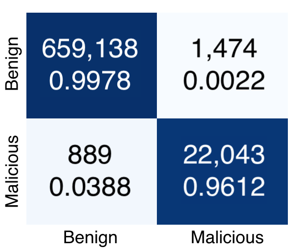
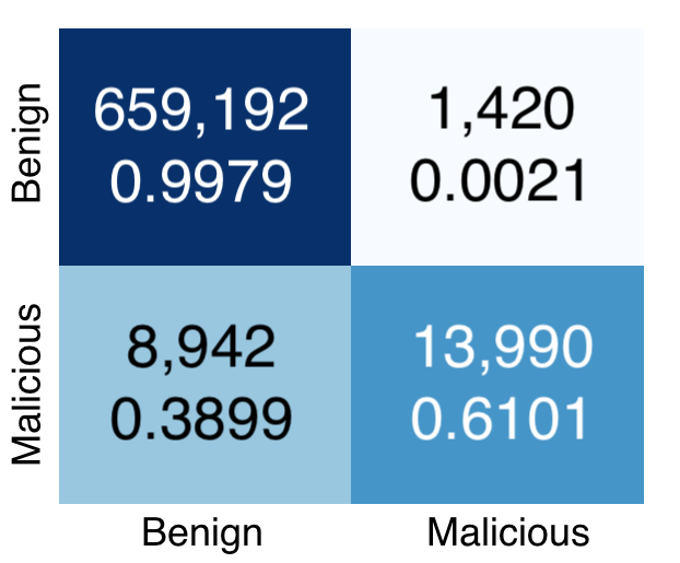

In order to answer the aforementioned question (ii), we train the deep learning model using some portion of the IP addresses. This is reasonable because DHCP typically operates in the same network, meaning that the network identity is static (e.g., the first 24-bit of IP addresses of a class C network).
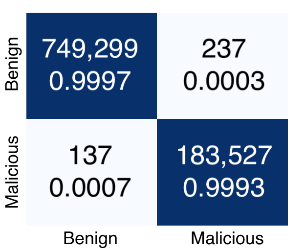
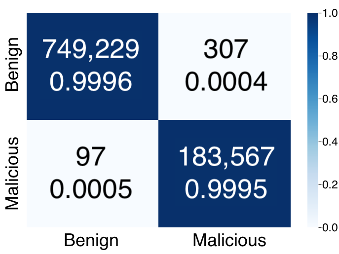
Figure 3 shows the results for the two datasets with and without IP address features. Figure 3(e) shows the results of using just the first three octets for source and destination IP address. In Figure 3(b) we observe that for the ISCX IDS 2012 dataset, when removing the IP address feature the performance drops considerably in terms of TPR and FNR. For the CIC IDS 2017 dataset, Figure 3(d) shows that removing the IP address only slightly degrades the performance in comparison to ISCX IDS 2012. Note that there is considerably larger amount of malicious examples in CIC IDS 2017 () compared to ISCX IDS 2012 (). We also notice that embedding the IP address with only the first three octets (Figure 3(e)) achieves similar results as when using the full IP address as shown (Figure 3(c)). This leads to the following:
Insight 2
DNN while using the first three octets of the IP address is as effective as using the full IP address, meaning that deep learning based intrusion detection is robust in the presence of DHCP. However, using full IP addresses is important when the dataset is imbalanced (i.e., the proportion of labeled malicious traffic is small).
III-D Using Autoencoders for network intrusion detection
III-D1 Pre-processing
For the Autoencoder experiments, all 69 usable continuous features of flow statistics in the CIC IDS 2017 dataset are used, and are normalized using the min-max technique mentioned above. One categorical feature of “protocol” is also used, which only has 3 unique values, and is converted to floating point numbers using one-hot encoding. The high-cardinality features of IP address and port are not used; we leave it to future work to incorporate these into the training of autoencoders.
III-D2 Training
The autoencoder configuration consists of 7 layers, with the first and last layer using the sigmoid activation function, and all other hidden layers using ReLU. The first and last layer consist of 72 units (representing all input features), and the hidden layers consist of 140, 35, 16, 16, 35 units respectively. In addition, L1 regularization is applied to the first input layer. The objective function for the autoencoder is the squared error. Written out in terms of weights and inputs, this function is shown in Eq. (3) below.
| (3) |
III-D3 Experiment and results
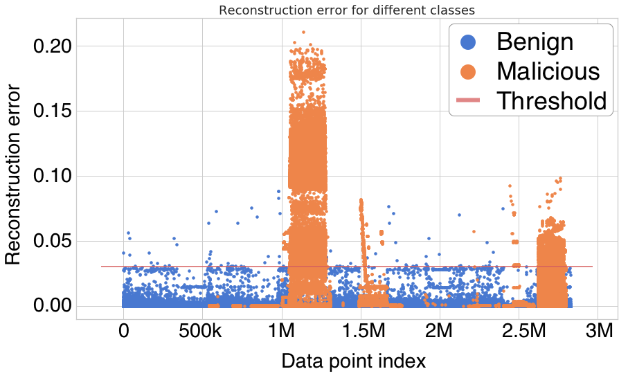
Figure 4 plots the experimental results. We observe that there is a higher reconstruction error for the malicious traffic flows as compared to the benign flows. Depending on the threshold set, the number of false positives can be adjusted. With the current threshold set at a reconstruction error, there only results in a total of false positives and a False-Positive Rate of . However, there is a high False-Negative Rate of . In addition, we observe that a majority of the malicious flows are clustered in groups, lending credence to future work that can incorporate the time domain as a feature. We draw the following insight:
Insight 3
Autoencoders can be effective as anomaly detection mechanisms for network intrusion detection (in terms of low False-Positive Rate) when training on benign traffic only.
IV Limitations
The present study has some limitations. From a methodology point of view, we only considered two kinds of neural networks. Future research needs to consider additional types of neural networks. For DNNs, we need to conduct further experiments using only the first two octets (first 16 bits), or even the first one octet, to see if they can achieve the same results as using the full 32-bit IP address. For Autoencoders, we need to investigate whether or not using the IP address and port features can reduce their False-Negative Rate. From a datasets point of view, the ISCX IDS 2012 dataset contains only binary ground-truth labels (i.e., malicious vs. benign) and contains no HTTP traffic.
V Conclusion
We have shown that DNN can achieve excellent results in supervised network intrusion detection. We also showed that using only the first three octets of IP addresses can be effective in coping with the use of dynamic IP addresses, indicating robustness of DNN in the presence of DHCP. We further showed that autoencoders can be used for anomaly detection when they are trained on benign flows.
Acknowledgements. This work was supported in part by ARL grant #W911NF-17-2-0127 and NSF CREST Grant #1736209.
References
- [1] F. Edgeworth, “Xli. on discordant observations,” The London, Edinburgh, and Dublin Philosophical Magazine and Journal of Science, vol. 23, no. 143, pp. 364–375, 1887.
- [2] D. E. Denning, “An Intrusion-Detection Model,” IEEE Transactions on Software Engineering, vol. SE-13, no. 2, pp. 222–232, 1987.
- [3] U. Fiore, F. Palmieri, A. Castiglione, and A. De Santis, “Network anomaly detection with the restricted boltzmann machine,” Neurocomputing, vol. 122, pp. 13–23, 2013.
- [4] “KDD Cup Dataset,” 1999. \urlhttp://kdd.ics.uci.edu/databases/kddcup99/kddcup99.html.
- [5] R. Sommer and V. Paxson, “Outside the Closed World: On Using Machine Learning for Network Intrusion Detection,” in 2010 IEEE Symposium on Security and Privacy, pp. 305–316, IEEE, 2010.
- [6] Y. Hyun, B. Huffaker, D. Andersen, E. Aben, C. Shannon, M. Luckie, and K. Claffy, “The caida ipv4 routed/24 topology dataset,” URL http://www.caida.org/data/active/ipv4_routed_24_topology_dataset.xml, 2011.
- [7] R. Lippmann, R. K. Cunningham, D. J. Fried, I. Graf, K. R. Kendall, S. E. Webster, and M. A. Zissman, “Results of the 1998 darpa offline intrusion detection evaluation,” in Proc. RAID, 1999.
- [8] R. Lippmann, J. W. Haines, D. J. Fried, J. Korba, and K. Das, “The 1999 darpa off-line intrusion detection evaluation,” Computer networks, vol. 34, no. 4, pp. 579–595, 2000.
- [9] M. Allman, M. Bennett, M. Casado, S. Crosby, J. Lee, B. Nechaev, R. Pang, V. Paxson, and B. Tierney, “Lbnl/icsi enterprise tracing project,” 2005.
- [10] I. Sharafaldin, A. Habibi Lashkari, and A. A. Ghorbani, “Toward Generating a New Intrusion Detection Dataset and Intrusion Traffic Characterization,” in 4th International Conference on Information Systems Security and Privacy, pp. 108–116, 2018.
- [11] A. Shiravi, H. Shiravi, M. Tavallaee, and A. A. Ghorbani, “Toward developing a systematic approach to generate benchmark datasets for intrusion detection,” Comput. Secur., vol. 31, pp. 357–374, May 2012.
- [12] W. Yassin, N. I. Udzir, Z. Muda, M. N. Sulaiman, et al., “Anomaly-based intrusion detection through k-means clustering and naives bayes classification,” in Proc. ICOCI, vol. 49, pp. 298–303, 2013.
- [13] A. Ammar, “A decision tree classifier for intrusion detection priority tagging,” Computer and Communications, vol. 3, no. 04, p. 52, 2015.
- [14] G. Folino, F. S. Pisani, and P. Sabatino, “A distributed intrusion detection framework based on evolved specialized ensembles of classifiers,” in Proc. ECAEC, pp. 315–331, 2016.
- [15] Z. Tan, A. Jamdagni, X. He, P. Nanda, R. P. Liu, and J. Hu, “Detection of denial-of-service attacks based on computer vision techniques,” IEEE transactions on computers, vol. 64, no. 9, pp. 2519–2533, 2015.
- [16] B. Atli, “Anomaly-based intrusion detection by modeling probability distributions of flow characteristics,” 2017.
- [17] A. Ahmim, L. Maglaras, M. A. Ferrag, M. Derdour, and H. Janicke, “A novel hierarchical intrusion detection system based on decision tree and rules-based models,” arXiv preprint arXiv:1812.09059, 2018.
- [18] M. De Gregorio and M. Giordano, “An experimental evaluation of weightless neural networks for multi-class classification,” Applied Soft Computing, vol. 72, pp. 338–354, 2018.
- [19] M. N. Adnan and M. Z. Islam, “Forest pa: Constructing a decision forest by penalizing attributes used in previous trees,” Expert Systems with Applications, vol. 89, pp. 389–403, 2017.
- [20] I. Ibarguren, J. M. Pérez, J. Muguerza, I. Gurrutxaga, and O. Arbelaitz, “Coverage-based resampling: Building robust consolidated decision trees,” Knowledge-Based Systems, vol. 79, pp. 51–67, 2015.
- [21] C.-C. Chang and C.-J. Lin, “Libsvm: Alibraryforsupportve ctormachines,” Availableat: http://www. csie. ntu. edu. tw/scjlin/libsvm, 2001.
- [22] J. Hühn and E. Hüllermeier, “Furia: an algorithm for unordered fuzzy rule induction,” Data Mining and Knowledge Discovery, vol. 19, no. 3, pp. 293–319, 2009.
- [23] D. Aksu, S. Üstebay, M. A. Aydin, and T. Atmaca, “Intrusion detection with comparative analysis of supervised learning techniques and fisher score feature selection algorithm,” in Proc. ISCIS, pp. 141–149, 2018.
- [24] D. Aksu and M. A. Aydin, “Detecting port scan attempts with comparative analysis of deep learning and support vector machine algorithms,” in IBIGDELFT’2018, pp. 77–80, 2018.
- [25] J. Jiang, Q. Yu, M. Yu, G. Li, J. Chen, K. Liu, C. Liu, and W. Huang, “Aldd: A hybrid traffic-user behavior detection method for application layer ddos,” in TrustCom/BigDataSE, pp. 1565–1569, 2018.
- [26] S. Ustebay, Z. Turgut, and M. A. Aydin, “Intrusion detection system with recursive feature elimination by using random forest and deep learning classifier,” in IBIGDELFT, pp. 71–76, 2018.
- [27] A. Pektaş and T. Acarman, “A deep learning method to detect network intrusion through flow-based features,” International Journal of Network Management, p. e2050.
- [28] M. Xu, K. M. Schweitzer, R. M. Bateman, and S. Xu, “Modeling and predicting cyber hacking breaches,” IEEE T-IFS, vol. 13, no. 11, pp. 2856–2871, 2018.
- [29] Z. Li, D. Zou, S. Xu, X. Ou, H. Jin, S. Wang, Z. Deng, and Y. Zhong, “Vuldeepecker: A deep learning-based system for vulnerability detection,” in Proc. NDSS’2018.
- [30] Z. Li, D. Zou, S. Xu, H. Jin, H. Qi, and J. Hu, “Vulpecker: an automated vulnerability detection system based on code similarity analysis,” in Proc. ACSAC’2016, pp. 201–213.
- [31] L. Xu, Z. Zhan, S. Xu, and K. Ye, “An evasion and counter-evasion study in malicious websites detection,” in Proc. IEEE CNS’14, 2014.
- [32] L. Xu, Z. Zhan, S. Xu, and K. Ye, “Cross-layer detection of malicious websites,” in ACM CODASPY’13, pp. 141–152, 2013.
- [33] Z. Zhan, M. Xu, and S. Xu, “Characterizing honeypot-captured cyber attacks: Statistical framework and case study,” IEEE T-IFS, vol. 8, no. 11, pp. 1775–1789, 2013.
- [34] Z. Zhan, M. Xu, and S. Xu, “Predicting cyber attack rates with extreme values,” IEEE Transactions on Information Forensics and Security, vol. 10, no. 8, pp. 1666–1677, 2015.
- [35] Y.-Z. Chen, Z.-G. Huang, S. Xu, and Y.-C. Lai, “Spatiotemporal patterns and predictability of cyberattacks,” PLoS One, vol. 10, 05 2015.
- [36] E. Ficke, K. M. Schweitzer, R. M. Bateman, and S. Xu, “Characterizing the effectiveness of network-based intrusion detection systems,” in IEEE MILCOM 2018, pp. 76–81, 2018.
- [37] S. Xu, “Cybersecurity dynamics,” in Proc. Symposium on the Science of Security (HotSoS’14), pp. 14:1–14:2, 2014.
- [38] S. Xu, “Cybersecurity dynamics: A foundation for the science of cybersecurity,” in Proactive and Dynamic Network Defense (Z. Lu and C. Wang, eds.), Springer New York, 2018 (to appear).
- [39] S. Xu, W. Lu, and L. Xu, “Push- and pull-based epidemic spreading in arbitrary networks: Thresholds and deeper insights,” ACM TAAS, vol. 7, no. 3, pp. 32:1–32:26, 2012.
- [40] X. Li, P. Parker, and S. Xu, “A stochastic model for quantitative security analysis of networked systems,” IEEE TDSC, vol. 8, no. 1, pp. 28–43.
- [41] W. Lu, S. Xu, and X. Yi, “Optimizing active cyber defense dynamics,” in Proc. GameSec’13, pp. 206–225, 2013.
- [42] S. Xu, W. Lu, L. Xu, and Z. Zhan, “Adaptive epidemic dynamics in networks: Thresholds and control,” ACM TAAS, vol. 8, no. 4, 2014.
- [43] Y. Han, W. Lu, and S. Xu, “Characterizing the power of moving target defense via cyber epidemic dynamics,” in Proc. HotSoS’14, 2014.
- [44] R. Zheng, W. Lu, and S. Xu, “Preventive and reactive cyber defense dynamics is globally stable,” IEEE TNSE, vol. 5, no. 2, 2018.
- [45] Z. Lin, W. Lu, and S. Xu, “Unified preventive and reactive cyber defense dynamics is still globally convergent,” IEEE/ACM Transactions on Networking, 2019 (accepted for publication).
- [46] M. Pendleton, R. Garcia-Lebron, J.-H. Cho, and S. Xu, “A survey on systems security metrics,” ACM Comput. Surv.
- [47] J. Cho, S. Xu, P. Hurley, M. Mackay, T. Benjamin, and M. Beaumont, “Stram: Measuring the trustworthiness of computer-based systems.” ACM Computing Survey, 2019.
- [48] P. Du, Z. Sun, H. Chen, J. Cho, and S. Xu, “Statistical estimation of malware detection metrics in the absence of ground truth,” IEEE T-IFS, vol. 13, no. 12, pp. 2965–2980, 2018.
- [49] J. D. Mireles, E. Ficke, J.-H. Cho, P. Hurley, and S. Xu, “Metrics towards measuring cyber agility.” IEEE T-IFS, 2019.
- [50] I. Goodfellow, Y. Bengio, and A. Courville, Deep Learning. MIT Press, 2016. \urlhttp://www.deeplearningbook.org.
- [51] C. Guo and F. Berkhahn, “Entity embeddings of categorical variables,” arXiv preprint arXiv:1604.06737, 2016.
- [52] Google, “Machine learning crash course: Embeddings.” \urlhttps://developers.google.com/machine-learning/crash-course/embeddings/video-lecture, 2019.
- [53] R. Thomas, “An introduction to deep learning for tabular data.” \urlhttps://www.fast.ai/2018/04/29/categorical-embeddings/, 2018.
- [54] A. H. Lashkari, G. D. Gil, M. S. I. Mamun, and A. A. Ghorbani, “Characterization of tor traffic using time based features,” in Proc. ICISSP, pp. 253–262, 2017.