A DECam View of the Diffuse Dwarf Galaxy Crater II: The Colour-Magnitude Diagram

Abstract

We present a deep Blanco/DECam colour-magnitude diagram (CMD) for the large but very diffuse Milky Way satellite dwarf galaxy Crater II. The CMD shows only old stars with a clearly bifurcated subgiant branch (SGB) that feeds a narrow red giant branch. The horizontal branch (HB) shows many RR Lyrae and red HB stars. Comparing the CMD with [Fe/H] = -2.0 and [$\alpha$/Fe] = +0.3 alpha-enhanced BaSTI isochrones indicates a mean age of 12.5 Gyr for the main event and a mean age of 10.5 Gyr for the brighter SGB. With such multiple star formation events Crater II shows similarity to more massive dwarfs that have intermediate age populations, however for Crater II there was early quenching of the star formation and no intermediate age or younger stars are present. The spatial distribution of Crater II stars overall is elliptical in the plane of the sky, the detailed distribution shows a lack of strong central concentration, and some inhomogeneities. The 10.5 Gyr subgiant and upper main sequence stars show a slightly higher central concentration when compared to the 12.5 Gyr population. Matching to Gaia DR2 we find the proper motion of Crater II: $\mu_{\alpha}\cos\delta$=-0.14 $\pm$ 0.07 , $\mu_{\delta}$=-0.10 $\pm$ 0.04 mas yr^-1, approximately perpendicular to the semi-major axis of Crater II. Our results provide constraints on the star formation and chemical enrichment history of Crater II, but cannot definitively determine whether or not substantial mass has been lost over its lifetime.

1 Introduction

Crater II (Torrealba et al., 2016) is an enigmatic object in the pantheon of normal and ultra-faint dwarf galaxies associated with our Galaxy. It occupies a parameter space where it is physically very large - with half light radius $1066\pm 84$ pc (Torrealba et al., 2016) so similar in size to classic dwarf galaxies such as Sculptor and Fornax - but 100 times less luminous with $M_{v}=-8.2$ (Torrealba et al., 2016), and of such low stellar density that its stars are difficult to discern from amongst Galactic foreground stars and faint background galaxies. In this latter characteristic it is similar to the ultra-faint dwarfs (UFD) and Simon (2019) draws the boundary between UFDs and more luminous dwarfs in the luminosity - metallicity plane close to the position of Crater II. The discovery of Antlia II (Torrealba et al., 2019) lying behind the Galactic disk and also of similar size and very low surface brightness might argue for a significant number of such galaxies still to be discovered. It is presently an open question as to how Crater II formed and subsequently evolved, with a key aspect being whether it has lost most of its original mass and, if not, how has it managed to remain intact for a Hubble time? Fritz et al. (2018) analysed the orbits of a number of Milky Way (MW) satellites by use of Gaia Data Release 2 (Gaia DR2, Gaia Collaboration 2018) proper motion determinations. For Crater II, they find a reconstructed orbit that is radial with eccentricity $\sim 0.7$ and with pericenter that may be less than 20 kpc from the center of the MW, depending on the adopted mass for the MW. Such an orbit, consistent with models by Sanders, Evans & Dehnen (2018); Fattahi et al. (2018), together with the observed size of Crater II, would suggest a system vulnerable to disruption. In addition, Fu, Simon & Alarcón Jara (2019) identify 37 Crater II members from radial velocities, 22 previously classified as members by Caldwell et al. (2017), and together with Gaia DR2 astrometry calculate an orbit for Crater II, concluding that it is almost certain that the galaxy has been stripped over its lifetime. Spectroscopy of Crater II members, mostly Red Giant Branch (RGB) and Asymptotic Giant Branch (AGB) stars (Caldwell et al., 2017; Fu, Simon & Alarcón Jara, 2019), demonstrates a resolved but rather narrow range of [Fe/H] values, suggesting a relatively simple chemical evolution, together with very cold dynamics although, despite this, apparently Crater II is dark-matter dominated with M/L = 53${}^{+15}_{-11}$ M_☉/L_V,☉ (Caldwell et al., 2017).

Studies of Crater II by our group and others (Joo et al., 2018; Monelli et al., 2018; Vivas et al., 2019), have identified a copious number of RR Lyrae (RRL) variable stars indicative of a strong ancient population. Importantly, RRL are useful for delineating the spatial distribution of the galaxy, and for large enough structures can determine the depth as well. In the case of Crater II, the RRL distribution could provide a strong observational constraint as to whether stars are still being lost (Vivas et al., 2019).

In this paper we study the star formation history of Crater II by analyzing a Colour Magnitude Diagram (CMD) that reaches well below the main sequence turn-off (MSTO) for the oldest population. A companion paper (Vivas et al., 2019) discusses the variable star content of Crater II, from the same set of observations. In § 2 we describe the observations and preparation of the data, in § 3 we discuss the features of the CMD and compare with theoretical isochrones, in § 4 we discuss the spatial distribution of Crater II stars, and by matching 80 stars classified as members and with low Gaia proper motion errors, we calculate the Crater II proper motion. In § 5 we relate the variable stars properties to the CMD results, and in § 6 we discuss the results and present our conclusions.

2 Observations and Data Reduction

The Crater II observations presented here derive from an allocation of three nights awarded by NOAO (P.I. A.R. Walker, prop-id 2017A-0210) with DECam on the Blanco 4m telescope at Cerro Tololo Inter-American Observatory (CTIO). From these observations we have produced a deep CMD and high-quality light curves for the Crater II variable stars, with main science goals to study the star formation history and the spatial distribution of the galaxy’s stellar populations. The observing log of the observations used for the CMD is summarized in Table 1. When the Moon was down we took exposures of 180s in a $u,g,i$ sequence, centered on the Crater II position as given by Torrealba et al. (2016) with small dithers to fill in the CCD gaps. If the Moon was up only $g,i$ exposures were taken. In photometric conditions SDSS standard star fields were observed, mostly equatorial.

Table 1: Log of the DECam observations

Run Date	$gi$ sequences	$ugi$ seq.	IQ (arcsec)	Comments
19 Mar 2017	9	38	$0.8-1.5$	some cloud
20 Mar 2017	10	44	$1.0-1.3$	clear
21 Mar 2017	13	39	$1.0-1.5$	clear

2.1 Image Combination

The images were processed by the DECam Community Pipeline (CP, Valdes 2014), which removes the instrument signature and provides various data products. For the specific purposes of this study custom stacks were produced, as follows: A total of 153 $g$, 153 $i$ and 32 $u$ band exposures were available, and after examination of the image quality and the depth of each of these exposures, stacks were produced containing 100, 100, 31 selected images in $g$, $i$, $u$ respectively, rejecting images that were taken in poor sky transparency, or with a very bright sky, or in poor seeing conditions. For these stacks, the CP produces multi-extension FITS (MEF) files that have 9 image extensions with each containing approximately 9K $\times$ 9K pixels and corresponding to $\sim$ 39 $\times$ 39 arcmin on the sky. The extensions are spatially arranged in a 3 $\times$ 3 format that covers the approximately circular 2 degree diameter DECam field, thus the four corner extensions (numbers 1, 3, 7, 9) are only partially filled by DECam.

Two alternative algorithms for flattening the sky background are offered by the CP. Here we chose to use the osj option rather than osi after visual inspection that the former skies were flatter with only minimal over-subtraction around very bright objects. The bad pixel masks provided for stacks are very simple, with a value 0 corresponding to good data, a value 1 coming from an input image bad pixel mask, and a value 2 (the majority of the bad pixels) coming from where there was no useful data, e.g. from a star saturated on all images. Of particular utility is the exposure map provided by the CP, that is, an image where the data are the exposure times corresponding to each pixel in the stacked object image.

We further processed the provided stacks in preparation for photometry, producing two sets of images as follows: the first full set had (i) any pixel appearing with a value of 1 or 2 in the bad pixel mask was replaced by 32767, the second uniform set had (i) any pixel appearing with a value of 1 or 2 in the bad pixel mask was replaced by 32767, in addition (ii) for all pixels in the exposure maps with value less than 16200 seconds ($g$, $i$) or 5040 seconds ($u$) the corresponding image pixel was replaced by 32767. The values of 16200 and 5040 seconds are 90% of the maximum possible exposure times for $g,i$ and $u$ respectively. The value of 32767 for the invalid pixel indicator was chosen for compatibility with the requirements of the photometry program (see below).

The observation scripts used for the Crater II exposures deliberately dithered the telescope just enough to fill in the gaps between the CCDs, with small additional random dithers of size a few arcsec arising from errors in the telescope pointing and adjustments made by the active optics system on an image by image basis to optimize image quality. The full data set will therefore contain stars, at a given magnitude, that have a range in $S/N$ due to a varying contribution of exposures. However for brighter stars (e.g. including the RRL at g $\sim$ 21) high $S/N$ is achieved even with only a few contributing exposures, and the photometric accuracy is dominated by systematic effects rather than shot noise. Therefore, for bright stars we have full spatial coverage with no drawbacks, and we can with confidence use the full dataset (74541 stars) for studying the morphology of Crater II as indicated by the RRL (Vivas et al., 2019). For the uniform set as described above with selection by exposure time, the sacrifice is that the coverage fraction is reduced to $\sim$ 60 percent (44294 stars) however the remaining good pixels are very uniform in depth. This is very important for correct interpretation of any changes in features in the faintest parts of the CMD as a function of spatial position.

In summary, from the above procedures we have produced two sets of three image FITS files, one each for $g$, $i$ and $u$, each file with 9 image extensions of approximately 9K $\times$ 9K pixels. The first set covers the full field with no gaps, and the second set is more restrictive, including $\sim$ 60 percent of the stars, but with uniformity and cleanness suitable for interpreting the photometry to the faintest levels.

2.2 Photometry

We use DAOPHOT (Stetson, 1987, 1994) for the photometry. Firstly, the DAOPHOT parameter files were prepared, of particular note is that we set the highest good pixel value ($hi$) = 15000 counts. While this is much less that the full-well values for any of the DECam CCDs, the CP does not explicitly correct for the brighter-fatter effect (Bernstein, et al., 2017) so it is preferable to keep stars selected to define the PSF and also those used for comparison with photometric standards to be those of no more than medium brightness. In any case, the brighter stars will all be Galactic foreground field stars and not of interest to this project. We searched for objects down to $S/N$ threshold ($th$) of 3.5, in two passes. For the center 9K $\times$ 9K field (extension 5, centered on Crater II), and considering the uniform sample that excludes the dithered regions, we found 42890, 60368, 1574 objects in $g$, $i$, $u$ respectively thus the object density for $g$, $i$ is approximately one per 90 arcsec², i.e. comfortably low.

The Blanco-DECam combination produces tight stellar images and a Moffat function with beta parameter = 3.5 is an excellent fit to the stellar image profiles, including the profile wings. After some experimentation we chose a linear-varying ($va=1$) PSF as being appropriate; while a quadratic-varying ($va=2$) PSF showed slightly smaller fit residuals for the PSF stars, the resulting photometry showed no improvement and we decided to keep the simpler functional form for the PSF. In itself, the ability to fit the stacks with a va=1 psf form is a simple confirmation that nothing untoward with regard to the star images is taking place spatially in the stacking process.

Following aperture photometry and PSF star picking, the PSF photometry was performed in the standard way with ALLSTAR. For each image the PSF was constructed from $\sim 200$ stars (100 for $u$). The photometric errors for the $g-i$ colors were calculated as the quadrature sum of the errors in $g$ and i returned by ALLSTAR, and were <0.01 mag for $g<21,<0.02$ mag for $g<22.5$, and averaged 0.04, 0.1, 0.2 mag at $g=24,25,26$ respectively. Since the depths achieved in $g$ and $i$ are similar, the errors in the $g$ and $i$ bands at these stated magnitudes will be approximately 2/3 of those for the colors. Exactly the same procedure was carried out on the two sets of images (uniform, full).

It is instructive to compare the approach chosen here (stack the images, then run DAOPHOT/ALLSTAR), to the alternative of running DAOPHOT/ALLSTAR/ALLFRAME on the individual images. In principle the latter forced-photometry approach should be superior (Stetson, 1994) and be able to go deeper since the star list is constructed from all available images. However the computation resources needed to handle 231 DECam images as opposed to 3 is very significant, and was beyond those available to our group, even when using PHOTRED (Nidever et al., 2017) to handle all the book-keeping and efficiently automate the process. By contrast, all the photometry for this project was run in a few minutes per image using a MacBook Pro laptop. The well-known difficulties for doing photometry on stacks, such as poor control of PSF across the field, poor control of errors, varying depth, are mitigated here by the low distortion and near-constant image quality across the DECam focal plane, by the similariry of the quantum efficiency response for the DECam CCDs over the passbands of main interest ($g$, $i$), and by use of the uniform set of reductions as described above for the critical interpretive tasks.

The photometric ($g$, $i$) calibration involved transformation to the SDSS system (Alam et al., 2015; Nidever et al., 2017) by cross-correlating low-error matches ($\sigma<0.05$ mag) at the catalogue level with the Crater II catalogue produced by PHOTRED (Nidever et al., 2017), see Vivas et al. (2019) for details on how the reference catalogue was produced. The SDSS and DECam $g$ and $i$ passbands are quite similar, and we find simple linear transformations, excluding stars with photometric errors $\sigma>0.05$ mag., and using S and D to denote SDSS and DECam respectively:

$$g_{S}-g_{D}=0.0710(\pm 0.0003)(g_{S}-i_{S})+0.0174(\pm 0.0004),N=7141$$ (1)

$$i_{S}-i_{D}=0.0783(\pm 0.0003)(g_{S}-i_{S})-0.0541(\pm 0.0004),N=7258$$ (2)

The $u$ band photometry was left on the DECam natural system, since our intent was to use these observations to select Crater II members –mostly RGB, AGB and Horizontal Branch (HB) stars– in $g$ vs. $g-i$ vs. $u-g$ space (Di Cecco et al., 2015). For this task it is not necessary to calibrate the $u$ band.

With the photometry in hand, we proceeded with an initial evaluation by constructing plots of the photometric errors as a function of magnitude, and plots of the PSF fit parameters chi and sharp as functions of magnitude. The former allowed formation of an envelope that included the great majority of detected objects but excluded those with large errors, and bounds on chi of $0,1$ fulfilled a similar function of removing errant measurements. Because of the high Galactic latitude of Crater II and the diffuse nature of the galaxy itself the star density is not so great as to make photometry difficult by having many overlapping stars, and thus the sharp parameter is a very efficient separator of stars and galaxies. We used $-0.5<sharp<0.2$ to select stars and $sharp>0.2$ to select galaxies. The samples appear to be very pure (referring here to $g$ and $i$, the shallower $u$ band images contain few galaxies) except in the final faintest one magnitude, where from the CMDs (see below) some stars are clearly classified as galaxies, and vice versa. With these definitions in hand, we proceeded to match stars between the photometric bands, taking account of the systematic few-pixel positional differences between the $g$, $i$, $u$ stacks, defining a successful match for objects with centers separated by no more than 3.5 pixels (0.9 arcsec). In the case of multiple matches, the closest was selected. With astrometry from the original images WCS and redefined using SAOImageDS9, the nine photometry files were merged into a single stellar photometric catalogue. By comparison, the galaxy photometric catalogue (i.e. that containing all objects with $sharp>0.2$) contains approximately four times as many objects as the stellar catalogue. The stellar catalogue is shown in Table 2, where we use flags to denote whether the object is in the uniform selection (F_uni = 1), is a variable star (F_var = 1), or is identified as a probable member on spectroscopic (F_spec = 1) or photometric grounds (F_phot = 1).

Table 2: Crater II Stellar Photometry Catalogue

ID	RA	Dec	g	$\sigma_{g}$	i	$\sigma_{i}$	E(B-V)SFD	Funi*	Fphot*	Fspec*	Fvar*
	(deg)	(deg)	(mag)	(mag)	(mag)	(mag)	(mag)
1	176.16106	-18.444340	19.1575	0.003	18.4130	0.005	0.038425	0	0	0	0
2	176.16196	-18.273500	25.3828	0.119	22.9508	0.029	0.040400	0	0	0	0
3	176.16199	-18.237010	24.7683	0.091	23.7151	0.063	0.040001	0	0	0	0
4	176.16278	-18.420690	21.6401	0.008	21.0008	0.008	0.039027	0	0	0	0
5	176.16293	-18.454950	25.0343	0.087	23.5285	0.045	0.038168	0	0	0	0
6	176.16348	-18.429810	25.6254	0.162	24.5563	0.115	0.038752	0	0	0	0
7	176.16354	-18.247700	23.4218	0.020	21.8672	0.012	0.040073	0	0	0	0
8	176.16368	-18.262930	22.2587	0.008	20.5067	0.005	0.040219	0	0	0	0
9	176.16371	-18.438970	20.8335	0.004	20.3301	0.006	0.038505	0	0	0	0
10	176.16373	-18.227880	24.9655	0.087	21.8863	0.010	0.039807	0	0	0	0
…	…	…	…	…	…	…	…	…	…	…	…
37914	177.32239	-18.648880	21.0050	0.039	20.7230	0.017	0.033798	0	0	0	1
37915	177.32240	-17.783121	17.8570	0.002	17.3552	0.002	0.030800	1	0	0	0
37916	177.32245	-17.446171	25.6924	0.091	24.2554	0.062	0.035800	1	0	0	0
37917	177.32245	-18.545030	24.5695	0.049	24.2915	0.076	0.032083	0	0	0	0
37918	177.32253	-18.674610	25.0724	0.094	24.7120	0.122	0.033977	0	0	0	0
37919	177.32253	-18.654630	24.0953	0.037	23.2545	0.036	0.033842	0	0	0	0
37920	177.32254	-18.543490	25.7842	0.123	23.5299	0.034	0.032056	0	0	0	0
37921	177.32256	-18.089280	25.3239	0.088	24.6449	0.106	0.033353	0	0	0	0
37922	177.32257	-18.374910	24.2701	0.030	23.9927	0.054	0.030500	1	0	0	0
37923	177.32257	-18.273441	23.7604	0.020	23.7887	0.048	0.033800	1	0	0	0
37924	177.32257	-18.932541	25.8975	0.117	25.3470	0.173	0.038400	1	0	0	0
37925	177.32262	-18.363504	24.0402	0.025	21.8884	0.007	0.030500	1	0	0	0
37926	177.32269	-18.632470	19.5170	0.003	18.3982	0.003	0.033608	0	1	1	0
37927	177.32269	-18.947861	25.5766	0.090	24.9110	0.121	0.038900	1	0	0	0
37928	177.32269	-18.797030	19.6891	0.003	18.2289	0.003	0.036104	0	0	0	0
…	…	…	…	…	…	…	…	…	…	…	…
74532	178.45450	-18.356200	23.5320	0.025	23.0068	0.028	0.037385	0	0	0	0
74533	178.45505	-18.378880	25.3801	0.109	24.3159	0.083	0.037335	0	0	0	0
74534	178.45630	-18.438780	22.4640	0.011	20.9631	0.011	0.039191	0	0	0	0
74535	178.45670	-18.398970	24.5338	0.065	22.3133	0.015	0.038049	0	0	0	0
74536	178.45689	-18.326450	21.8885	0.008	19.4466	0.004	0.037705	0	0	0	0
74537	178.45721	-18.385570	23.5345	0.027	22.8753	0.025	0.037589	0	0	0	0
74538	178.45842	-18.466220	24.1100	0.039	21.2650	0.009	0.039506	0	0	0	0
74539	178.45905	-18.396870	25.5048	0.117	24.2044	0.084	0.038045	0	0	0	0
74540	178.45979	-18.365350	24.4644	0.053	21.8250	0.012	0.037323	0	0	0	0
74541	178.46194	-18.465880	24.5687	0.069	22.5059	0.020	0.039691	0	0	0	0

• *F_uni, F_phot, F_spec, and F_var are flags that show if a particular star has been identified in the uniform catalogue, as photometric member, as spectroscopically-confirmed star, and as variable star member, respectively.

• Notes.- Table 2 is published in its entirety in the machine-readable format. A portion is shown here for guidance regarding its form and content.

3 The Colour Magnitude Diagram

3.1 Reddening Correction

We first correct the Crater II photometry for foreground reddening, obtaining E($B$-$V$) from the Schlegel, Finkbeiner & Davis (1998) interstellar dust maps using the python task dustmaps (Green, 2018). Although the reddening is small due to the high Galactic latitude, the very large field of DECam usually means that the reddening varies across the field, and so this aspect should be taken into account (see Figure 1). In order to apply the reddening correction, we correct each $g$ and $i$ magnitude of our detected sources using the Schlegel, Finkbeiner & Davis (1998) reddening values and the coefficients given in Schlafly & Finkbeiner (2011), i.e. A_g = 3.303 E($B$-$V$), A_i = 1.698 E($B$-$V$). The same procedure was applied in the companion paper (Vivas et al., 2019).

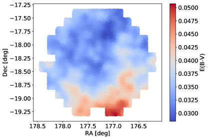
Figure 1: Interstellar dust reddening map from Schlegel, Finkbeiner & Davis (1998) of the central $\sim$3 sq. deg. of Crater II observed with DECam.

The reddening-corrected $i,g-i$ CMDs are shown in Figure 3, where results for both the full and uniform reductions are displayed, each of the two sets of three panels depict stars within a elliptical distance of 0.35 degrees of the center of Crater II, between 0.35 and 0.65 degrees, and exterior to 0.65 degrees. We denote these inner, central, and outer regions, respectively.

3.2 CMD Description

The CMD (Figure 3) reaches to $g,i\sim 25.5$ and the stellar sequences belonging to Crater II are thus defined to well below the level of the oldest MSTO. Crater II stars are prominent in the inner and central regions, while the outer region is dominated by field stars. In the outer region of the DECam field, compact and relatively blue galaxies dominate in numbers over both field and Crater II stars for magnitudes fainter than $i\sim 24.5$. With low $S/N$ some galaxies will have measured value of DAOPHOT $sharp<0.2$ and will thus be classified as stars, and given the relative numbers, will appear on the CMD. It is notable that this contamination is less prominent in the uniform sample than for the full sample, as expected since the uniform sample will exclude stars with low $S/N$ for a given magnitude. Over the whole field, compact galaxies outnumber stars by a factor three, but as previously discussed a cut on DAOPHOT sharp excludes these with high efficiency except near the faint magnitude cutoff.

Crater II shows a strongly populated HB in the vicinity of the RRL, the latter are relatively easy to see on the CMD since they are bluer than the majority of field stars. There are red HB (RHB) stars, much more contaminated by MSTO field stars than the RRL. There is a likely increase in density of the RHB stars of stars near the red end of the RHB. There appear to be no blue HB (BHB) stars at all, and this is consistent with the RRL distribution, see discussion in Vivas et al. (2019). The RGB is narrow, down to the base, however the subgiant branch (SGB) is clearly split into two components, both feeding into the RGB. There is an indication that the brighter SGB is less prominent at larger radii, this will be discussed in the following section. There are many blue stragglers, but no turn-off brighter than the two just described is visible.

The Crater II AGB stars and RGB stars brighter than the HB are difficult to discern from amongst the foreground field stars, even in the inner regions. However there are three ways in principle that we can identify Crater II stars in the field-star dominated regions of the CMD.

Firstly, we can cross reference our photometry to stars classified as members by Caldwell et al. (2017); Fu, Simon & Alarcón Jara (2019) on the basis of radial velocity and metallicity; we call this the spectroscopic membership sample. There are a total of 70 stars in this sample, 56 of them are in Caldwell et al. (2017) and 35 in Fu, Simon & Alarcón Jara (2019), with 21 stars in common between both catalogues. It is worth noting that, by definition, this is a very pure sample.

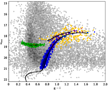
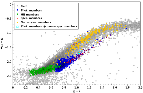
Figure 2: Left.- ($u_{\rm inst}$, $g-i$) colour-magnitude diagram of the sources contained within the DECam FoV centered on Crater II. Field stars are shown in grey, photometric members in blue (AGB+RGB) and in green (HB), spectroscopically confirmed members as red crosses and spectroscopically confirmed non-members in yellow. Cyan open squares display those stars that were classified in this work as photometric members of Crater II but they are not members from the spectroscopy. A 12.5 Gyr isochrone of [Fe/H] = -2.0 dex is plotted for guidance. Right.- Colour-colour diagram for the same sources. The spectroscopically confirmed non-members are located in the region of the more metal-rich stars, while the members of Crater II are in the region of the most metal-poor stars.

Secondly, we have $u$ band photometry for all stars to below the level of the HB, and so can select for stars that are metal-poor in the two-colour diagram, and also lie close to the cluster sequences in the CMD. In order to separate candidates and field stars, we followed the prescription described by Di Cecco et al. (2015) and Calamida et al. (2017). Briefly, we generated two isodensity maps in the $i$, $u-g$ and in the $g,u-g$ CMDs and created two ridge lines that helped us to locate our most probable candidates. These candidates were selected considering those stars located between $\pm$1$\sigma$ (defined as the quadratic sum of the photometric errors in the three bands) to the 3D ridge line and their position in the ($u-g$), ($g-i$) diagram. We selected a total of 1166 stars that we call the photometric catalogue. This method is expected to work well for AGB and RGB stars because the magnitude of these stars in the $g$ and $i$ bands is a strong function of the colour, and thus provides an effective constraint. We can select HB stars similarly, although the small range in luminosity makes field star discrimination less effective. Figure 2 shows, in the left panel, the ($u_{\rm inst}$, $g-i$) CMD and, in the right panel, the ($u_{\rm inst}-g$) versus ($g-i$) colour-colour diagram for the selected photometric membership sample with blue (RGB+AGB) and green (HB) dots while red crosses represent the spectroscopic membership sample.

We can test for field star contamination in the RGB and AGB photometric catalogue (863 stars) in the following way: Caldwell et al. (2017) in their table 2 list all their observed stars, and have provided probabilities (private communication to M. Monelli) that each star is a Crater II member. All except a very few stars are classified as member (probability 1) or non-member (probability 0), see Caldwell et al. (2017) for details of how they calculate the probability. There are 314 stars with probability 0, represented as yellow dots in Figure 2. We cut off our photometric catalogue at $i=20.1$ to match the spectroscopic catalogue, leaving 157 stars, and search for positional matches; we find five (cyan open squares in Figure 2) stars with positional agreements 0.2-0.3 arcsec using a 5 arcsec window. With the areas of the two catalogues differing by a factor 2.0, then the contamination in our catalogue of RGB and AGB stars is thus 5 $\times$ 2 / 157 = 0.06. This analysis does assume that the fainter stars in our photometric catalogue have the same degree of field star contamination as do those brighter than $i=20.1$ but this is a reasonable assumption, see Figure 2. We note that one of the five stars is metal poor, [Fe/H] = -1.67 and with a radial velocity indicating a non-member, is apparently a halo giant at approximately the distance of Crater II. The remaining four stars are non members on the grounds of both metallicity and radial velocity.

The photometric sample also contains 303 RHB stars. Unfortunately, we have no way of testing spectroscopically for membership in any significant way, with only two RHB stars in the Fu, Simon & Alarcón Jara (2019) catalogue. Membership can be evaluated by counting field stars in photometric (magnitude, colour) boxes above and below the RHB. This is complicated by the high density of field stars, and the rapid change of star density as a function of colour as the MSTO colour for the foreground stars is approached. We conclude that the photometric catalogue for the RGB and AGB stars is pure at the 95% level, but the RHB star entries (303 stars) will be contaminated by field stars at a much higher level, and one that is difficult to estimate.

Thirdly, we have the variable star members. In our companion paper (Vivas et al., 2019), we have identified a total of 106 variable star members of Crater II which consist of 98 RRL, seven Anomalous Cepheid (AC), and one dwarf Cepheid (DC) stars. This sample is also considered a very pure.

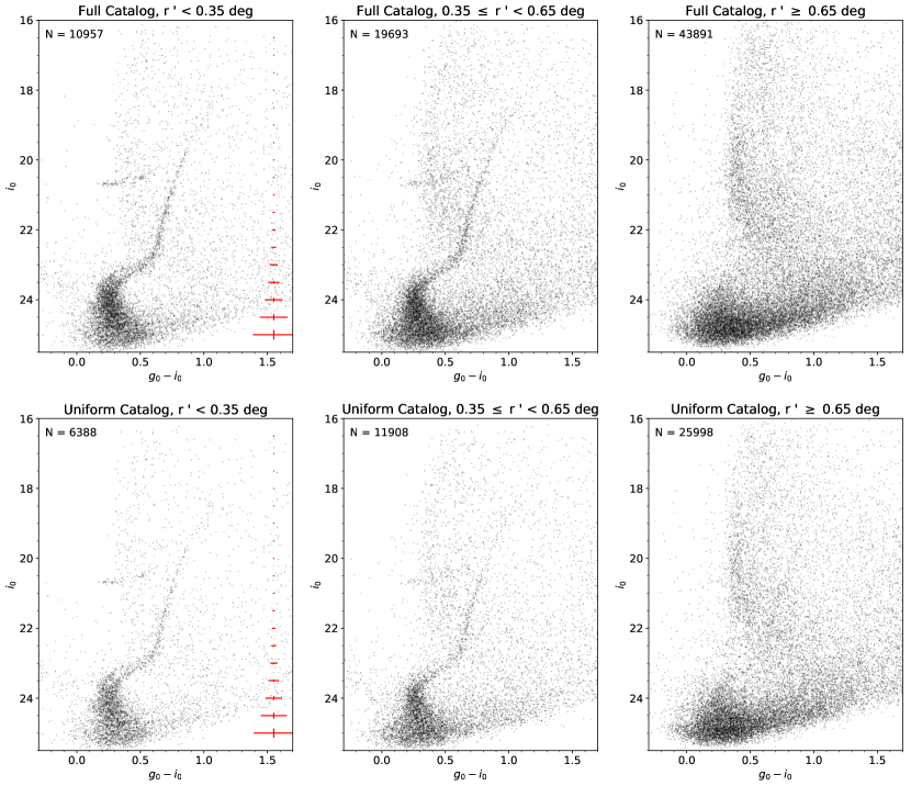
Figure 3: Colour-Magnitude diagrams of Crater II. Top and bottom panels represent the full and the uniform catalogues, respectively (see the text for details). Left panels show those stars within 0.35°elliptical distance (see text for details) centred on Crater II, middle panels display those stars within 0.35°and 0.65°, while right panels show those stars beyond 0.65°.

3.3 Isochrone Comparison to the CMD

The BaSTI (Hidalgo et al., 2018) model grid selected for the present analysis corresponds to that of stellar evolutionary computations accounting for the occurrence of mass loss (according to the Reimers’ law and the free parameter $\eta$ set to the value of 0.3) as well as for core convective overshooting during the central H-burning stage and atomic diffusion. However core convective overshooting is irrelevant in the present context since low-mass (i.e. old) stars burn H into a radiative core. In Figure 4 we compare the CMD sequences with alpha-enhanced (Pietrinferni et al. in prep.) BaSTI isochrones and zero-age horizontal branch (ZAHB) models.

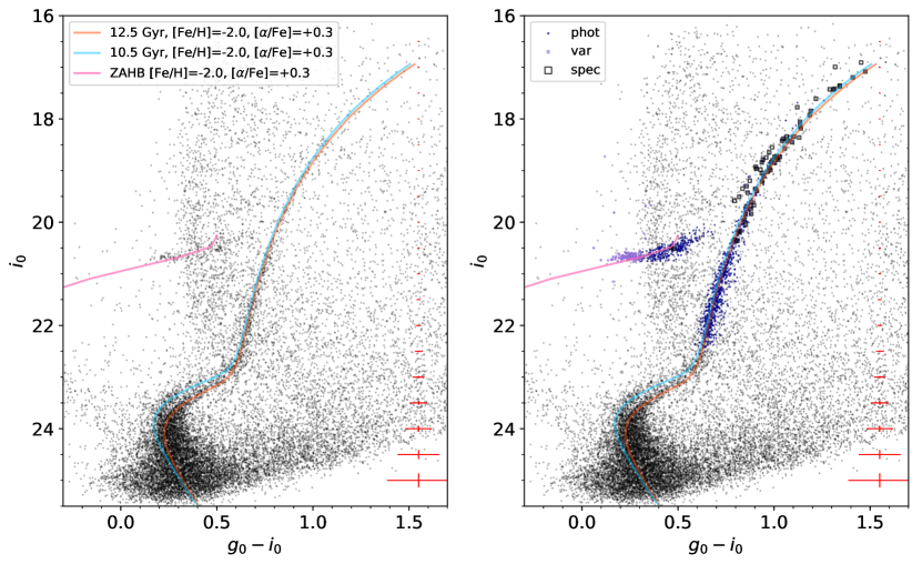
Figure 4: Isochrone Comparison to the CMD of Crater II (r’ $<$ 0.78°, 1.5$\times$r_h). The CMD was corrected star-by-star by the Schlegel, Finkbeiner & Davis (1998) reddening map, using the modified version of Schlafly & Finkbeiner (2011). Orange and light blue lines represent the best set of [Fe/H]=-2.0 alpha enhanced ([$\alpha$/Fe]=+0.3) isochrones from BaSTI (Pietrinferni et al. in preparation) that match the CMD of Crater II, 12.5 Gyr and 10.5 Gyr respectively. Isochrones and ZAHB were shifted using a distance modulus for Crater II of 20.33 mag (Vivas et al., 2019). Additionally, we add 0.04 mag to the total reddening in order to make the isochrones and the stellar sequences match better (see text for more details). Spectroscopic members are shown as black squares in the right panel, while photometric members are displayed as dark blue dots and variable members (RR Lyrae stars, Anomalous Cepheids, dwarf Cepheid) are purple dots.

The spectroscopy by Caldwell et al. (2017); Fu, Simon & Alarcón Jara (2019) finds mean [Fe/H] = -2.0 with a small dispersion (sigma $\sim 0.2\pm 0.1$ dex). With Crater II lying near the boundary between UFDs and classical dwarfs (Simon, 2019), we assume that Crater II will behave similarly with respect to alpha element enhancement. All these galaxies, at the metallicity of Crater II or lower, are alpha-enhanced (Kirby, et al., 2011; Vargas, et al., 2013; Simon, 2019) with the transition from high alpha to solar alpha ratio driven by the change from dominance of SN II to SN Ia, and showing variance from galaxy to galaxy depending on the details of the star formation history for each. For Crater II a choice of [$\alpha$/Fe] = +0.3 would seem appropriate. We therefore choose BaSTI-IAC alpha-enhanced isochrones (Pietrinferni et al. in preparation) with [Fe/H] = -2.0 and [$\alpha$/Fe] = +0.3, after exploring parameter space quite widely. In matching the isochrones and the ZAHB to the data we use the most recent RRL distance modulus ($\mu_{0}$ = 20.333 $\pm$ 0.004 mag, Vivas et al. 2019), and apply a small colour shift of 0.04 magnitude so that the isochrones better coincide with the observational sequences. The origin of this colour shift could be one or more of small errors in the reddening scale, errors in the photometric zeropoints, or a residual shortcoming in the adopted colour-effective temperature scale adopted for transferring the isochrones from the theoretical plane to the observational one.

The right panel of Figure 4 shows that the photometric (dark blue dots) and spectroscopic (black open squares) members of Crater II play an important role when doing the isochrone matching. The age of the isochrone that best matches the older turnoff is 12.5 Gyr and the younger SGB is best matched with an isochrone with the same metallicity and an age of 10.5 Gyr. The latter is a minority population, and given the errors in the individual spectroscopic measurements for the stars classed as Crater II members, we cannot rule out that the 10.5 Gyr stars might have slightly lower alpha elements abundance and slightly higher [Fe/H] than does the 12.5 Gyr population, a scenario similar to that convincingly demonstrated for the Carina dwarf galaxy by VandenBerg, Stetson & Brown (2015). If, for example, we compare a solar-scaled isochrone with [Fe/H] = -1.7 (Hidalgo et al., 2018) to the younger population then an excellent match is obtained, although at an age 1 Gyr younger (9.5 Gyr) than the alpha enhanced isochrone.

Similarly, while there is no obvious evidence for older (12.5 - 13.5 Gyr) stars, the lack of sensitivity of the RGB colour to metallicity for metal poor stars, the age-metallicity degeneracy, and the unknown alpha element enhancement for such stars, make it possible to hide such a minority population. We return to this issue in § 6.

Note that the isochrones are placed on the centre of the star distributions in the CMD; compared to the magnitude errors at the level of the SGBs both appear to be broadened in age. The younger population is close to, or under, the age limit of 10-11 Gyr for forming RRL (Walker, 1989; Glatt et al., 2008; Catelan, 2018), and is thus expected to contain few or no RRL, with the majority of the core-helium burning stars populating the RHB.

3.4 The Horizontal Branch Morphology

We consider an inner region with r’ $<$ 35 arcmin (see § 4.2) within which we count 0 BHB, 43 RRL and 80 RHB stars, and (see Table 3) 530 stars from the older SGB and 233 from the younger. The older SGB will populate the RHB and RRL, while the younger SGB will likely only populate the RHB, if so we calculate that 43 RRL and 42 RHB stars belong to the 12.5 Gyr population and 38 RHB stars belong to the 10.5 Gyr population. We calculate the HB morphology parameter (Lee, 1990) for the 12.5 Gyr population to be $\frac{\rm{N(BHB)}-\rm{N(RHB)}}{\rm{N(BHB)}+\rm{N(RRL)}+\rm{N(RHB)}}=-0.49$.

As demonstrated by Lee et al. (1994) and Sarajedini, Lee & Lee (1995) for Galactic globular clusters, a HB dominated by RRL and RHB stars with few or no BHB stars can be produced by high metal abundance, clearly not the case here, but also by young age. For a metal poor population such as Crater II, an age of the RRL of 11-12 Gyr after applying a small zeropoint offset, accounting for the modern age of the Universe (13.8 Gyr), to the results of Lee et al. (1994) and Sarajedini, Lee & Lee (1995), is consistent with the observed HB morphology, but suggesting an age slightly younger than found by our isochrone fitting.

Other parameters that can affect the HB morphology are He abundance enhancements or spread, or a non-canonical value for the mass loss on the RGB. After the discovery of multiple stellar populations in globular clusters there is compelling evidence (Milone, et al., 2014) that, after metallicity and age, He abundance anomalies play a major role in determining HB morphology. However for Crater II such anomalies would produce BHB stars, which are not observed. For mass loss, McDonald & Zijlstra (2015) show for a large sample of globular clusters that there is little dispersion in the measurements. We will proceed for Crater II by making the assumption that age and metallicity are driving the HB morphology, as there is no evidence from the available data that more exotic explanations are required.

3.5 The CMD and the RR Lyrae Variables

Joo et al. (2018); Monelli et al. (2018); Vivas et al. (2019) show that the Crater II RRL period distribution is unusual with only a few RRcd stars and many RRab. This distribution implies that a 12.5 Gyr stellar population, during the core He-burning stage, is not able to populate the whole RR Lyrae domain from the blue edge of the First Overtone instability strip to the red boundary of the Fundamental strip. In this respect Crater II is similar to the unusual Galactic globular cluster Ruprecht 106 (Dotter et al., 2018), which is young, metal-poor and contains only RRab variables (Buonanno, Corsi, Pecci, Richer & Fahlman, 1993; Kaluzny, Krzeminski & Mazur, 1995; Leaman, VandenBerg & Mendel, 2013).

By considering the dispersion in brightness in the $i$-band RRL period-luminosity (PL) relation, and dividing the RRab stars into bright (B) and faint (F) groups by considering the position of each star relative to the mean PL relation, Vivas et al. (2019) show that the two groups have a different spatial distribution with the F group more centrally concentrated (their figure 12). This is interpreted as a small difference in the mean metallicity (nominally 0.17 dex) between the two groups. We do note, considering the spectroscopic sample of stars and removing the AGB stars, the RGB stars are almost all closer than 0.02 mag in colour to the fitted isochrone (Figure 4). The BaSTI isochrones show that a small systematic metallicity shift of 0.1-0.2 dex could be hidden in the present observations particularly if combined with a slight age change (e.g. a few 100 Myr) given the well-known degeneracy between RGB age and metallicity, in the sense that younger age will produce a bluer RGB and higher metallicity will make the RGB redder.

Additionally, we plotted a C_ugi diagram (Monelli, et al., 2013) for the Crater II RGB stars with spectroscopy, this pseudo-colour can split stars with different metalliicities over much of the RGB. We divided the stars into two groups divided by [Fe/H] = -2.0, and found no significant difference between the location of the two groups of stars in this diagram. We conclude that we are not able, with the photometry alone, to provide further insight into the possible metallicity gradients in Crater II suggested by Vivas et al. (2019).

4 Crater II Structure and Motion

4.1 Proper Motion

All proper motion measurements are from Gaia DR2 (Gaia Collaboration, 2018). Figure 5 has three panels, the left panel shows the 2D proper motion distribution for stars in an external field comprising an annulus with radii of 1.5 and 2.0 deg centered on Crater II, the center panel shows the 2D proper motions distribution for stars inside r < 1.0 deg, and the right panel is the subtraction between the first two panels (normalized) that clearly reveals Crater II. Guided by this, we proceed by selecting stars in our catalogue that satisfy the following criteria: they are flagged as photometric, spectroscopic, or variable star members; they are found in Gaia DR2 with proper motion errors smaller than 1 mas yr^-1; and they have proper motions between $\pm 3$ mas yr^-1 mas yr^-1 (both in RA and Dec). This gives a sample of 80 stars, which are displayed as orange symbols in Figure 6, of which 50 have spectroscopy and thus also appear in proper motion analyses by Fritz et al. (2018); Fu, Simon & Alarcón Jara (2019), 65 are photometric members (of which 36 have spectroscopy), and 1 AC. The proper motion of Crater II is then determined by a weighted average of the proper motions for these 80 stars, in units of mas yr^-1, $\mu_{\alpha}\cos{\delta}=-0.14$ $\pm$ 0.07 (standard deviation = 0.66), $\mu_{\delta}=-0.10$ $\pm 0.04$ (standard deviation = 0.38), represented by a blue square in Figure 6. This Crater II systemic proper motion, using a slightly larger sample of stars, is consistent within the errors with the two previous Gaia derived proper motions (Fritz et al. 2018: $\mu_{\alpha}\cos{\delta}$ = -0.18 $\pm$ 0.06, $\mu_{\delta}$ = -0.11 $\pm$ 0.03 from 58 Caldwell et al. 2017 spectroscopic members; Fu, Simon & Alarcón Jara 2019: $\mu_{\alpha}\cos{\delta}$ = -0.17 $\pm$ 0.06, $\mu_{\delta}$ = -0.07 $\pm$ 0.07 from 37 of their spectroscopic members).

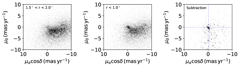
Figure 5: Left.- Proper motions of a field region defined by a circular ring of 1.5°$<$ r $<$ 2.0°centered on Crater II. Middle.- Proper motions of a circular area inside r $<$ 1.0°centered in Crater II. Right.- The subtraction between left and middle panel reveal the proper motion of Crater II. The intersection of the two dashed blue lines marks the locus of the proper motion determined by the members of Crater II (see text for details).

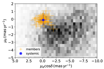
Figure 6: Proper motions of the Crater II photometric, spectroscopic, and variable members (orange) present in our catalogue whose proper motion errors are smaller than 1 mas yr^-1. The blue square shows the systemic proper motions of Crater II obtained from the selected (80) stars: $\mu_{\alpha}\cos{\delta}$ = -0.14 $\pm$ 0.07 mas yr^-1, $\mu_{\delta}$ = -0.10 $\pm$ 0.04 mas yr^-1. The grey scale map shows the proper motions of a field mostly outside Crater II, defined by a region of 1.5°$<$ r $<$ 2.0°centered on Crater II.

4.2 The Spatial Distribution of Crater II stars

The GB stars (RGB + AGB) of Crater II overall have an elliptical distribution similar to that found for the RRL by Vivas et al. (2019), the parameters of which we have adopted for the analysis in this section. In Figure 7 we show the distribution and the morphology for the 863 GB stars from the photometric sample together with the proper motion vector obtained in § 4.1.

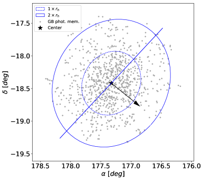
Figure 7: Spatial distribution of the giant branch (RGB + AGB) stars considered photometric members (grey dots) of Crater II. Morphological parameters were calculated using a robust bivariate normal distribution fit to these stars. The ellipticity (0.12) and position angle (135°) of the blue ellipses located at 1 and 2$\times$ r_h (Torrealba et al., 2016) come from the results of this fit. The new recalculated center of Crater II is marked with a black star. The blue line points to the direction of the semi-major axis, while the black arrow indicates the proper motion direction of Crater II derived in this work ($\mu_{\alpha}\cos\delta$=-0.14 $\pm$ 0.07 mas yr^-1, $\mu_{\delta}$=-0.10 $\pm$ 0.04 mas yr^-1).

The distribution of the members of Crater II (see § 3.2) does not show a peaked central concentration, also suggested from the distribution of RRL (Vivas et al., 2019) and confirmed by the larger sample of stars here. Although overall the distribution of stars is smooth, on closer examination there are indications of inhomogeneities in the spatial distribution of stars. Figure 8, an isodensity contour map, shows two overdensities located at (RA = 177.45 deg, DEC = -18.47 deg) and (RA = 177.18 deg, DEC = -18.40 deg). They are approximately the same distance from the Crater II center (displayed as a black cross), and between these two peaks, in the center of Crater II, there is a 2-$\sigma$ fall in the number of stars. The reliability of these overdensities is statistically confirmed by calculation of Poisson uncertainties.

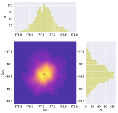
Figure 8: Isodensity contour map and RA and DEC distributions of the members (photometric + spectroscopic + variables) of Crater II.

There is an indication from Figure 3 that there may be a difference in the relative numbers of the two SGB populations as a function of the elliptical distance (r’), and we investigate this further by selecting stars from the SGB and the top of the MS region of the CMD (from $i$ = 22.8 to $i$ = 24.3). We follow up the 10.5 Gyr isochrone with a circular bin of radius 0.02 mag, and with a circular bin of radius 0.03 mag for the 12.5 Gyr isochrones. At the ends of the region under consideration the two tracks are close enough so the stars may appear in both selections, in such cases the closest isochrone is selected so that there is no double counting. The selection performed is shown in Figure 9.

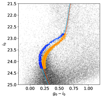
Figure 9: Zoom-in of the MS, SGB and lower RGB of the colour-magnitude diagram of Crater II. Orange (blue) dots represent the older (younger) MS-SGB stars selected under the criteria described in the text.

We then use the center of Crater II and the elliptical shape as defined by the RRL (Vivas et al., 2019) and divide into three annuli, the inner contains stars with elliptical distance (r’) less than 0.35 degrees, the second with elliptical distances between 0.35 and 0.65 degrees, and the outer with elliptical distances between 0.70 and 0.78 degrees. Although there are Crater II stars across the whole DECam field, their numbers in this outer annulus will be very few compared to the field stars, and for the MSTO region a good approximation for the purposes of this calculation is zero Crater II stars, however we conservatively consider an error of 10 percent in the outer annulus (field) star counts when using this number to correct the inner and center annulus star counts for field star contamination. For stars definitely identified as Crater II members such as the RRL, no corrections are required for comparing their star counts in the two inner annuli, and the errors quoted derive from the counts only.

Table 3: Radial Distributions of Crater II Stars

Population	Inner Annulus	Center Annulus	Outer Annulus	Normalised Inner	Normalised Center	Ratio Inner/Center
RR all	43	33				$1.3\pm 0.4$
RRab bright	12	17				$0.7\pm 0.4$
RRab faint	27	12				$2.2\pm 1.1$
12.5 Gyr	656	692	122	530	383	$1.38\pm 0.15$
10.5 Gyr	266	208	32	233	127	$1.83\pm 0.15$
Area (deg2)	0.2925	0.7163	0.2827

The results in Table 3 highlight the difference between the central concentration of faint and bright RRL, shown as a radial plot in figure 12 of Vivas et al. (2019). This has been interpreted as a slightly more metal poor population having a wider spatial distribution than the more metal rich stars. In any case, the spread in metallicity between the two populations is expected to be small. In addition, we confirm by star counts the visual impression that the SGB plus upper MS stars that follow the 10.5 Gyr isochrone appear slightly more centrally concentrated than those that follow the 12.5 Gyr isochrone. For more populous dwarf galaxies it is commonly found that younger populations are more centrally condensed than older populations (see e.g. Harbeck, et al., 2001; Tolstoy, et al., 2004; Okamoto, et al., 2017), although generally the age differences are greater than for Crater II. While it is suggestive here to make an association between the two populations of SG-MSTO stars and the apparent two groups of RRL stars, a direct association is not supported on stellar evolution grounds as discussed above, and the ratios in Table 3 have large error bars. However, the radial distributions of the RRL and the two SG-MSTO stars are not inconsistent, in a scenario of a small increase of metallicity over a rather narrow age range. Spectroscopy of the HB stars, possible with present large telescopes, would help to turn the tentative statements from the present data into firmer conclusions.

5 Crater II Variable Stars Progenitors

The RRL variables are discussed by Joo et al. (2018); Monelli et al. (2018); Vivas et al. (2019), with the latter paper providing a definitive analysis of the pulsational properties. The distribution and relation of the RRL to other CMD components are discussed above. In addition to the 99 RRL (98 measured from DECam data), seven ACs and one DC have been found in Crater II by Vivas et al. (2019). With the large numbers of blue stragglers (BS) and no young stars, the DC is interpreted as an SX Phoenicis variable, and its discovery amongst the BS stars is not surprising, indeed there are likely to be more of these (very faint and short period) stars waiting discovery. For the AC, there are two production channels (Bono, Caputo, Santolamazza, Cassisi & Piersimoni, 1997; Fiorentino & Monelli, 2012; Cassisi & Salaris, 2013), the first is from an intermediate age population that directly produces the $1-2\ M_{\sun}$ stars, and for which there is no progenitor evidence from the Crater II CMD, while the second channel is from BS stars. This route also has two possible production channels, both involving merging of two stars; in globular clusters stellar collisions in the dense cluster core will be frequent, however this route is clearly not significant for Crater II. Instead, the coalescence of close binaries will be the production channel relevant here (Gautschy & Saio, 2017).

6 Discussion and Conclusions

From analysis of a deep CMD, and by comparison with the properties of the RRL discussed in detail in a companion paper (Vivas et al., 2019) we can make a number of statements about this unusual, but perhaps not uncommon, galaxy.

The main new finding in this paper has been possible thanks to the unprecedentedly deep CMD, which reaches the old MSTO with high photometric precision. The stellar populations of Crater II are characterized by two main events of star formation that occurred at a mean age of 12.5 and 10.5 Gyr ago. An old ($\sim 13.5$ Gyr) population seems to be a minor component, as disclosed by the main sequence isochrone fitting, by the HB morphology, which lacks a blue component, and by the characteristics of the RRL variable star population. These characteristics of the stellar population of Crater II (M_V = -8.2) are very unusual among UFDs; a similarly extended period of star formation in a UFD has been found so far only in the M31 satellite And XVI (Monelli, et al. 2016; M${}_{V}=-7.3$), even though in that case a double star-formation episode is not evident in the CMD, while it is hinted in the star formation history derived through CMD fitting. What may be the origin of a stellar component with such unusual characteristics? To try to answer this question, we will consider other observed aspects of this galaxy.

Firstly, the Crater II proper motion confirmed here, and the orbit that has been derived (Fritz et al., 2018; Fu, Simon & Alarcón Jara, 2019) suggest strongly that Crater II should be disrupting due to penetrating well into the more central regions of our Galaxy on each orbit. From the current analysis, we can state, in contrast, that the galaxy structure seems regular, and the younger (10.5 Gyr) population is more centrally concentrated than the older (12.5 Gyr) population, as is common in dwarf galaxies (Harbeck, et al., 2001; Tolstoy, et al., 2004; Okamoto, et al., 2017), which would support a quiet rather than an episodically violent life. However, we cannot make strong direct statements about this scenario, as a much wider area survey for extra tidal material, in particular RRL, would be needed to provide observational proof.

In this scenario, a relatively minor old population could be explained by preferential tidal stripping in the earliest pericentric passages (see e.g. Fritz et al. 2018 for an orbit integration under different assumptions of the Milky Way potential). The second event of star formation could have occurred or even have been triggered by one of these early pericentric passages, before complete removal of gas would have taken place, while the prior star formation events are consistent with star formation occurring along the orbit of the galaxy. This is behavior that is expected from simulations (see, e.g. Nichols, Revaz & Jablonka 2015 or Hausammann, Revaz & Jablonka 2019) and that has been observed, for example, in the Sagittarius dSph, which has retained gas and continued star formation during several pericentric passages prior to infalling (Siegel, et al., 2007).

An alternative scenario would be that Crater II is a relatively recent capture by our Galaxy; a relatively low initial star formation rate could indicate that it formed in an environment isolated from other galaxies. Gallart et al. (2015) suggested that the difference between dwarf galaxies with fast evolution (in fast dwarfs, star formation would have started early, probably before reionization and would have terminated early) compared to slow evolution (low intensity of early star formation, which then takes place for most or all of a Hubble time) depended on the density of the environment at time of formation, with fast evolvers forming in high density environments.

If the low amount of old population in Crater II is intrinsic (that is, not due to preferential stripping of the old population), it implies that the rate of star formation was low prior to reionization, and by this Crater II would comply with one of the criteria to be classified as a slow dwarf. However, the relatively early cessation of star formation $\sim$10 Gyr ago is at odds with the normal definition of a slow dwarf.

A combination of the two scenarios is however plausible. Given the high eccentricity of the derived orbit, and the expected orbital changes along the evolution in live haloes (Nichols, Revaz & Jablonka, 2015), the early distance of Crater II to the Milky Way may have been in excess of the currently measured 116.5 kpc (Vivas et al., 2019), and thus, it would have formed in a relatively isolated environment. In fact, even its currently calculated apocenter is similar to that of Milky Way dSph satellites such as Carina or Fornax that show extended star formation and were classified by slow dwarfs by Gallart et al. (2015). Its apocenter is also not unlike the estimated current distance between M31 and And XVI. Given the more eccentric orbit of Crater II compared to Carina and Fornax, the closer perigalacticon, possibly combined with the lower mass, would have resulted in a more efficient stripping of the gas in Crater II than in the other two galaxies, and thus resulted in an earlier cessation of its star formation. Some characteristics betraying the slow nature of Crater II may still noticeable. The observational search for stripping remnants mentioned above, and a detailed star formation history, carefully dealing with field star subtraction and modeling the HB and MSTO - SGB regions in particular, will help to better delineate the evolutionary history of this intriguing galaxy.

References

- Alam et al. (2015) Alam, S., et al. 2015, ApJS, 219, 12
- Bernstein, et al. (2017) Bernstein G. M., et al., 2017, PASP, 129, 114502
- Bono, Caputo, Santolamazza, Cassisi & Piersimoni (1997) Bono G., Caputo F., Santolamazza P., Cassisi S., Piersimoni A., 1997, AJ, 113, 2209
- Buonanno, Corsi, Pecci, Richer & Fahlman (1993) Buonanno R., Corsi C. E., Pecci F. F., Richer H. B., Fahlman G. G., 1993, AJ, 105, 184
- Calamida et al. (2017) Calamida A., et al., 2017, AJ, 153, 175
- Caldwell et al. (2017) Caldwell, N., Walker, M.G., Mateo, M., 2017, ApJ, 815, 117
- Cassisi & Salaris (2013) Cassisi S., Salaris M., 2013, Old Stellar Populations: How to Study the Fossil Record of Galaxy Formation. Wiley, New York
- Catelan (2018) Catelan M., 2018, IAUS, 11, IAUS..334
- Di Cecco et al. (2015) Di Cecco A., et al., 2015, AJ, 150, 51
- Dotter et al. (2018) Dotter A., Milone A. P., Conroy C., Marino A. F., Sarajedini A., 2018, ApJL, 865, L10
- Fattahi et al. (2018) Fattahi, A., et al., 2018, MNRAS, 476, 3816
- Fiorentino & Monelli (2012) Fiorentino G., Monelli M., 2012, A&A, 540, A102
- Fiorentino et al. (2015) Fiorentino, G., et al., 2015, ApJ, 798, 12
- Fritz et al. (2018) Fritz T. K., et al., 2018, A&A, 619, A103
- Fu, Simon & Alarcón Jara (2019) Fu S. W., Simon J. D., Alarcón Jara A. G., 2019, ApJ, 883, 11
- Gaia Collaboration (2018) Gaia Collaboration, arXiv:1804.09365
- Gallart et al. (2015) Gallart, C., et al., 2015, ApJ, 811, 18
- Gautschy & Saio (2017) Gautschy A., Saio H., 2017, MNRAS, 468, 4419
- Glatt et al. (2008) Glatt, K., et al., 2008, A.J., 135, 1106
- Green (2018) Green, G. M., 2018, Journal of Open Source Software, 3(26), 695
- Harbeck, et al. (2001) Harbeck D., et al., 2001, AJ, 122, 3092
- Hausammann, Revaz & Jablonka (2019) Hausammann L., Revaz Y., Jablonka P., 2019, A&A, 624, A11
- Hidalgo et al. (2018) Hidalgo, S.L., et al., ApJ, 856, 125
- Ivezić, Connelly, VanderPlas & Gray (2014) Ivezić Ž., Connelly A. J., VanderPlas J. T., Gray A., 2014, Statistics, Data Mining, and Machine Learning in Astronomy, Princeton Series in Modern Observational Astronomy
- Joo et al. (2018) Joo, S.-J., et al., 2018, ApJ, 861, 23
- Kirby, et al. (2011) Kirby E. N., Cohen J. G., Smith G. H., Majewski S. R., Sohn S. T., Guhathakurta P., 2011, ApJ, 727, 79
- Lee et al. (1994) Lee, Y.-W., Demarque, P., Zinn, R., 1994, Ap.J., 423, 248
- Lee (1990) Lee Y.-W., 1990, ApJ, 363, 159
- Kaluzny, Krzeminski & Mazur (1995) Kaluzny J., Krzeminski W., Mazur B., 1995, AJ, 110, 2206
- Leaman, VandenBerg & Mendel (2013) Leaman R., VandenBerg D. A., Mendel J. T., 2013, MNRAS, 436, 122
- McDonald & Zijlstra (2015) McDonald, I., Zijlstra, A.A., 2015, MNRAS, 448, 502
- Milone, et al. (2014) Milone A. P., et al., 2014, ApJ, 785, 21
- Monelli, et al. (2013) Monelli M., et al., 2013, MNRAS, 431, 2126
- Monelli, et al. (2016) Monelli M., et al., 2016, ApJ, 819, 147
- Monelli et al. (2018) Monelli, M., et al., 2018, MNRAS, 479, 4279
- Nichols, Revaz & Jablonka (2015) Nichols M., Revaz Y., Jablonka P., 2015, A&A, 582, A23
- Nidever et al. (2017) Nidever, D.L., et al., 2017, AJ, 154, 199
- Okamoto, et al. (2017) Okamoto S., et al., 2017, MNRAS, 467, 208
- Sanders, Evans & Dehnen (2018) Sanders J. L., Evans N. W., Dehnen W., 2018, MNRAS, 478, 3879
- Sarajedini, Lee & Lee (1995) Sarajedini A., Lee Y.-W., Lee D.-H., 1995, ApJ, 450, 712
- Schlafly & Finkbeiner (2011) Schlafly, E.F., & Finkbeiner, D.P., 2011, ApJ, 737, 103
- Schlafly et al. (2018) Schlafly, R.F., Green, G.M., Lang, D., 2018, ApJS, 234,39
- Schlegel, Finkbeiner & Davis (1998) Schlegel D. J., Finkbeiner D. P., Davis M., 1998, ApJ, 500, 525
- Scolnic et al. (2015) Scolnic, D., Casertano, S., Riess, A., 2015, ApJ, 815, 117
- Siegel, et al. (2007) Siegel M. H., et al., 2007, ApJL, 667, L57
- Simon (2019) Simon, J.D., 2019, ARA&A, 57, 375
- Stetson (1987) Stetson, P.B., 1987, PASP, 99, 191
- Stetson (1994) Stetson, P.B., 1994, PASP, 106, 250
- Tolstoy, et al. (2004) Tolstoy E., et al., 2004, ApJL, 617, L119
- Tonry et al. (2012) Tonry, J.L., Stubbs, C.W., Lykke, K.R., 2012, ApJ, 750, 99
- Torrealba et al. (2016) Torrealba, G., Koposov, S.E., Belokurov, V, Irwin, M., 2016, MNRAS, 459, 2370
- Torrealba et al. (2019) Torrealba, G., Belokurov, V., Koposov, S.E., 2019, MNRAS, 488, 2743
- Valdes (2014) Valdes, F., Gruendl, R., DES Project, 2014, ASPC, 485, 379
- VandenBerg, Stetson & Brown (2015) VandenBerg D. A., Stetson P. B., Brown T. M., 2015, ApJ, 805, 103
- Vargas, et al. (2013) Vargas L. C., Geha M., Kirby E. N., Simon J. D., 2013, ApJ, 767, 134
- Vivas et al. (2019) Vivas, A.K., et al., 2019, submitted
- Walker (1989) Walker, A.R., 1989, PASP, 101, 570