Subsystem-based Approach to Scalable Quantum Optimal Control

Abstract

The development of quantum control methods is an essential task for emerging quantum technologies. In general, the process of optimizing quantum controls scales very unfavorably in system size due to the exponential growth of the Hilbert space dimension. Here, I present a scalable subsystem-based method for quantum optimal control on a large quantum system. The basic idea is to cast the original problem as a robust control problem on subsystems with requirement of robustness in respect of inter-subsystem couplings, thus enabling a drastic reduction of problem size. The method is in particular suitable for target quantum operations that are local, e.g., elementary quantum gates. As an illustrative example, I employ it to tackle the demanding task of pulse searching on a 12-spin coupled system, achieving substantial reduction of memory and time costs. This work has significant implications for coherent quantum engineering on near-term intermediate-scale quantum devices.

Precise and complete control of multiple coupled quantum systems plays a significant role in the development of modern quantum science and engineering Brif et al. (2010); Letokhov (2007); D’Alessandro (2008); Dong and Petersen (2010); Acín et al. (2018). In particular, achieving control with high fidelity lies at the heart of enabling scaled quantum information processing. Quantum optimal control (QOC) is a subject aimed at finding a control law of optimal performance in steering the dynamics of a quantum system to some desired goal. Because of its ability to produce high-accuracy quantum operations, QOC has become a standard tool for various experimental platforms, ranging from nuclear magnetic resonance (NMR) Khaneja et al. (2005); Hogben et al. (2011), nitrogen-vacancy centers in diamond Dolde et al. (2014); Geng et al. (2016), ultracold atoms Rosi et al. (2013), to superconducting qubits Kelly et al. (2014); Zahedinejad et al. (2015); Machnes et al. (2018) and trapped ions Choi et al. (2014). In the past decades, a great effort has been put in developing fast and practical QOC methods Lloyd and Montangero (2014); Egger and Wilhelm (2014); Day et al. (2019); Machnes et al. (2018); Borzì et al. (2017). It turns out that, apart from certain simple cases where analytical solutions are available Khaneja et al. (2001, 2002); Lapert et al. (2010), QOC in general has to exploit numerical optimization techniques. A variety of optimization algorithms have been developed and demonstrated to be powerful in solving QOC problems, to name a few, gradient ascent pulse engineering (GRAPE) Khaneja et al. (2005), differential evolution Zahedinejad et al. (2015), machine learning Bukov et al. (2018), etc. They have their respective advantages in respect of algorithmic simplicity, convergence speed, or numerical stability. However, there is a critical difficulty of scalability that limits their success to only small-sized quantum devices. The process of control optimization often relies on heavy computational simulations of the dynamics of the system under control. The fact that the dimensionality of the tensor product Hilbert space grows exponentially with the system size can render an optimal control search algorithm computationally intractable. Currently, there have been put forward only a few strategies attempting to address this issue, including the use of tensor-network-based techniques Doria et al. (2011); Ma et al. and the hybrid quantum-classical approach Li et al. (2017); Lu et al. (2017).

In this work, I propose a simple subsystem-based approach to large quantum system optimal control. In this approach, the entire system is divided into a group of subsystems, and the entire system Hamiltonian is accordingly decomposed as intra-subsystem Hamiltonian plus inter-subsystem Hamiltonian. As constraints of subsystem-based optimization, the control pulse should implement all corresponding target operations of the subsystems with high fidelity, and meanwhile needs to be robust to the couplings between the subsystems. In general, a pulse that is designed on the subsystems without consideration for the inter-subsystem couplings does not necessarily implement the desired unitary on the whole system. The essential point here is that, if the pulse has robustness, then its global control fidelity should deviate only slightly with respect to its fidelities on the subsystems. It is noted that the idea of subsystem-based QOC has been previously considered in Ref. Ryan et al. (2008), but the approach adopted therein lacks a solid theoretical basis and thus is quite empirical. Here, I develop a methodology in transforming a large-sized QOC problem into a collective robust control problem on the subsystems. Furthermore, I show that the robust control problem can be effectively solved by a modified GRAPE algorithm under the Van Loan differential equation framework that was recently developed in Ref. Haas et al. .

It is worth pointing out that the feasibility of the approach crucially relies on assuming that the inter-subsystem couplings can be treated as perturbation terms. In principle, the validity of the assumption is relevant to how the full system is divided. Yet from a practical aspect of view, this assumption is reasonable because a realistic physical architecture normally has limited qubit connectivity (e.g., nearest-neighbor couplings only) like that shown in Fig. 1. The couplings between distant qubits are more likely to be weaker than those between adjacent qubits. This fact makes it possible to keep the subsystems small, and thence the problem size would grow only polynomially. To demonstrate the potential of the subsystem-based QOC method, I optimize pulses for elementary quantum gates on an NMR 12-qubit multiple coupled system. The results show that, due to the avoidance of simulations on the full system, the method is able to offer orders of magnitude speedup in finding pulses with around $99\%$ fidelities.

Figure 1: Schematic of a block architecture. Physically, it is appropriate to assume that the longer range couplings are negligibly small. This forms a sound basis for dividing the entire architecture into blocks. Each block represents a subsystem of coupled qubits, and the single arrows in between represent inter-subsystem couplings. Subsystem-based QOC performs pulse optimization on the subsystems, it has a much reduced problem scaling.

Subsystem-based QOC.—To start, I describe the basic problem setting. Consider an $n$-qubit quantum system $S$ described by a system Hamiltonian $H_{S}$. The task is to implement a desired unitary operation $\overline{U}$. Our framework restricts considerations to local quantum gates that operate on only a few qubits at a time. More general quantum operations can be decomposed into an array of simpler local quantum gates. We divide the system into $s$ disjoint subsystems $S=S_{1}\cup\cdots\cup S_{s}$. The choice of the division is governed by two considerations: (i) there are only a few comparatively small couplings between the subsystems, and (ii) the qubits that $\overline{U}$ operates on belong to the same subsystem, so that one can write $\overline{U}=\overline{U}_{S_{1}}\otimes\cdots\otimes\overline{U}_{S_{s}}$. With this subsystem division, the system Hamiltonian can now be written as

$$H_{S}=H_{0}+H_{1}=\sum_{k=1}^{s}H_{S_{k}}+\sum_{k<j}^{s}H_{S_{k}S_{j}},$$ (1)

where $H_{S_{k}}$ is the internal Hamiltonian of subsystem $S_{k}$, and $H_{S_{k}S_{j}}$ is the interaction Hamiltonian between $S_{k}$ and $S_{j}$. We denote the Hilbert space of the $k$th subsystem $S_{k}$ as $\mathcal{H}_{S_{k}}$, so $\left\{H_{S_{k}}\right\}$ are operators on $\mathcal{H}_{k}$, and $\left\{H_{S_{k}S_{j}}\right\}$ are operators on $\mathcal{H}_{S_{k}}\otimes\mathcal{H}_{S_{j}}$. To steer the system towards the desired operation, we add coherent controls based on externally applied control fields $u(t)$ ($0\leq t\leq T$). Often, the control fields are coupled with the individual qubits, hence we shall assume that the control Hamiltonian takes the form $H_{C}(t)=\sum_{k}H_{C_{k}}(t)$, in which $H_{C_{k}}(t)$ is the control Hamiltonian of subsystem $S_{k}$. The basic approach to the optimal control problem for the whole system is to search for a pulse shape $u(t)$ to

$$\max\quad F=\left|\operatorname{Tr}(U(T)\overline{U}^{\dagger})\right|^{2}/d^{2},$$ (2)

s.t. $$\dot{U}(t)=-i[H_{S}+H_{C}(t)]U(t).$$

where $F$ is the fidelity function, $d=\dim\mathcal{H}$, and $U$ starts from the identity operation $U(0)=\bm{1}_{d}$.

The basic idea of our approach is to consider a related robust quantum control problem. That is, we solve the optimal control problem for the intra-subsystem Hamiltonian $H_{0}$, and at the meantime require the control solution be robust to the inter-subsystem Hamiltonian $H_{1}$. For now, we denote $U(t)$ as the propagator generated by $H_{0}+H_{C}(t)$, and view $H_{1}$ as a variation of the generator. Let $\mathcal{D}_{U(T)}(H_{S_{k}S_{j}})$ denote the directional derivative of the propagator $U(T)$ with respect to the variation in $H_{0}+H_{C}(t)$ in the direction $H_{S_{k}S_{j}}$, as given by

$$\mathcal{D}_{U(T)}(H_{S_{k}S_{j}}) =\lim_{\epsilon\to 0}\frac{U(T,\epsilon)-U(T)}{\epsilon}$$

$$=\left.\frac{d}{d\epsilon}\right|_{\epsilon=0}\mathcal{T}e^{-i\int_{0}^{T}dt\left[H_{0}+H_{C}(t)+\epsilon H_{S_{k}S_{j}}\right]}$$

where $\mathcal{T}$ is the time-ordered operator. Then, robustness in $H_{1}$ can be achieved via maximizing the fidelity function $f=\left|\operatorname{Tr}(U(T)\overline{U}^{\dagger})\right|^{2}/d^{2}$ and minimizing the norm of every directional derivative $f_{S_{k}S_{j}}=\left\|\mathcal{D}_{U(T)}(H_{S_{k}S_{j}})\right\|^{2}/d^{2}$. Now, a critical observation is that it suffices to perform computations on just the subsystems. First, notice that for any time $t$, $U(t)$ can be factorized as $U(t)=U_{S_{1}}(t)\otimes\cdots\otimes U_{S_{s}}(t)$, where $U_{S_{k}}(t)$ is the propagator of subsystem $S_{k}$ generated by $H_{S_{k}}+H_{C_{k}}(t)$, therefore $f$ equals to the product of the fidelities of the subsystems $f=\prod_{k=1}^{s}f_{S_{k}}$. As to the directional derivatives, there is

$$f_{S_{k}S_{j}} =\left\|-iU(T)\int_{0}^{T}dtU^{\dagger}(t)H_{S_{k}S_{j}}U(t)\right\|^{2}/d^{2}$$

$$=\left\|\mathcal{D}_{U_{S_{k}}(T)\otimes U_{S_{j}}(T)}(H_{S_{k}S_{j}})\right\|^{2}/d^{2}_{\mathcal{H}_{S_{k}}\otimes\mathcal{H}_{S_{j}}}.$$

Here, the first line can be obtained via the Dyson series Dyson (1949); Haas et al. . Therefore, $f_{S_{k}S_{j}}$ can be evaluated simply on the pair of subsystems $S_{k}$ and $S_{j}$. More details about the derivation can be found in the Supplementary Material Sup .

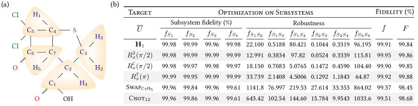
Figure 2: (a) Molecular structure of per-¹³C-labeled dichlorocyclobutanone. It contains 7 labeled carbon nuclei and 5 proton nuclei and hence forms a 12-qubit coupled system. The spins are coupled via through-bond interaction, so those spins that are not connected via chemical bonds would have smaller coupling strengths. (b) Subsystem-based pulse optimization. The method is tested for a number of different kind of local target operations. Here, $\mathbf{H}$ is the Hadamard gate, $R^{k}_{x}(\theta)$ denotes a rotational gate that rotates qubit $k$ about the $x$ axis with rotational angle $\theta$. As defined in the main text, $f$ and $F$ is the pulse fidelity in terms of subsystem Hamiltonian $H_{0}$ and full system Hamiltonian $H_{S}$, respectively.

Summarizing the above analysis, the robust control problem is essentially a multi-objective optimization problem on subsystems

$$\max\quad \Phi=\prod_{k=1}^{s}f_{S_{k}}-\sum_{k<j}^{s}\lambda_{kj}f_{S_{k}S_{j}},$$ (3)

s.t. $$\dot{U}_{S_{k}}(t)=-i[H_{S_{k}}+H_{C_{k}}(t)]U_{S_{k}}(t).$$

Here, the fitness function $\Phi$ is chosen as a linear combination of the objective functions, with $\lambda_{kj}$ being the positive weight coefficients associated to individual objectives. The weights will be tuned within an iterative algorithmic procedure. Since $f_{S_{k}S_{j}}\geq 0$, there must be $\Phi\leq 1$, so maximizing $\Phi$ close to 1 will imply a solution to the robust control problem Eq. (6), which also provides a solution to the original problem Eq. (5). This constitutes the central result of this work.

Now let us turn our attention to the solution method of the problem Eq. (6). There have been developed a variety of quantum optimal control algorithms. In particular, GRAPE, a gradient-based technique, is widely used for its good convergence speed and high numerical accuracy. In GRAPE, the optimization consists of iteratively executing two major steps. First the gradient of the fitness function with respect to the control parameters is computed, and then one determines an appropriate step length along a gradient-related direction. The algorithm continues until, an optimal solution is found or a termination criterion is satisfied. For the present problem, suppose the pulse $u(t)$ is discretized into $M$ slices of equal length $\tau=T/M$ and that the $m$th slice being of constant magnitude $u[m]$, then the key step is to compute the gradient $\partial\Phi/\partial u[m]$. To this end, I follow the methodology developed by Ref. Haas et al. , which extends the Shrödinger equation to a so-called Van Loan block matrix differential equation by which means the same gradient-based algorithm can apply. Concretely, define a set of operators $\left\{L_{S_{k}S_{j}}:1\leq k<j\leq s\right\}$ and $\left\{L_{C_{k}}(t):k=1,\ldots,s\right\}$ by

$$L_{S_{k}S_{j}} =\left[\begin{matrix}H_{S_{k}}+H_{S_{j}}&H_{S_{k}S_{j}}\\ 0&H_{S_{k}}+H_{S_{j}}\\ \end{matrix}\right],$$

$$L_{C_{k}}(t) =\left[\begin{matrix}H_{C_{k}}(t)&0\\ 0&H_{C_{k}}(t)\\ \end{matrix}\right].$$

They are referred to as Van Loan generators Loan (1978); Carbonell et al. (2008). Construct the Van Loan differential equation as

$$\dot{V}_{S_{k}S_{j}}(t)=-i[L_{S_{k}S_{j}}+L_{C_{k}}(t)+L_{C_{j}}(t)]V_{S_{k}S_{j}}(t),$$

then there is for $V_{S_{k}S_{j}}(t)$ the following expression

$$V_{S_{k}S_{j}}(t)=\left[\begin{matrix}U_{S_{k}S_{j}}(t)&\mathcal{D}_{U_{S_{k}S_{j}}(t)}(H_{S_{k}S_{j}})\\ 0&U_{S_{k}S_{j}}(t)\\ \end{matrix}\right].$$

Based on the above formula, the problem Eq. (6) is therefore essentially to optimize the following fitness function

$$\Phi=\prod_{k=1}^{s}f_{S_{k}}-\sum_{k<j}^{s}\lambda_{kj}\left\|V^{(1,2)}_{S_{k}S_{j}}(T)\right\|^{2}/d^{2}_{\mathcal{H}_{S_{k}}\otimes\mathcal{H}_{S_{j}}},$$ (4)

in which $V^{(1,2)}_{S_{k}S_{j}}(T)$ is the $(1,2)$ block sub-matrix of $V_{S_{k}S_{j}}(T)$. As observed by Ref. Haas et al. , since the Van Loan equation has the same general form as the Schrödinger equation, which implies that Eq. (7) still belongs to the class of bilinear control theory problems Elliott (2009), thus evaluation of $\partial\Phi/\partial u[m]$ can be done in the same way as how gradients are estimated in GRAPE. More details about the derivations and the algorithmic procedure can be found in the Supplementary Material Sup .

Optimal control on a 12-qubit NMR system.—The utility of the developed scheme can be demonstrated with a 12-qubit NMR molecule (¹³C-labeled dichlorocyclobutanone) Lu et al. (2017); Li et al. (2019). This is to date the largest spin quantum information processor with full controllability; see Supplemental Materials for its Hamiltonian parameters Sup . Running GRAPE for as large as a 12-qubit system involves computing of $2^{12}$-dimensional matrix exponentials and matrix multiplications as well, which requires a substantial amount of memory and time cost. The subsystem-based approach circumvents this difficulty. To see this, I divide the whole system into four subsystems, $S_{1}=\left\{\text{C}_{1},\text{C}_{2},\text{H}_{4}\right\}$, $S_{2}=\left\{\text{C}_{3},\text{H}_{2},\text{H}_{3}\right\}$, $S_{2}=\left\{\text{C}_{4},\text{C}_{5},\text{H}_{1}\right\}$, and $S_{4}=\left\{\text{C}_{6},\text{C}_{7},\text{H}_{5}\right\}$, each consisting of three spins; see Fig. 2(a). Instead of searching on the whole system, I perform pulse optimization on these subsystems, and consider pulse robustness to the inter-subsystem couplings $\left\{H_{S_{k}S_{j}}\right\}$ ($1\leq k<j\leq 4$). In this way, the optimization process involves only $2\times 2^{6}$-dimensional matrix operations. The results are shown in Fig. 2(b); more data are given in Supplementary Material Sup . From the simulations, several features can be identified. First, for a particular target operation, larger inter-subsystem couplings would result in larger perturbations to the ideal operation. Second, if a pulse has longer time length, the inter-subsystem couplings will have larger effects to the controlled evolution, and it will be harder to enhance the robustnes. On the whole, for the optimized pulses, the decreases from their full system fidelities to their corresponding subsystem fidelities are smaller than 1%. This confirms the capability of the subsystem-based algorithm in producing high-fidelity controls.

Discussions and Outlook.—The key insight behind the subsystem-based QOC method is the recognization that a practical physical system should have limited range couplings, so subsystem-based strategies can apply. Although all-to-all connected qubit graph may facilitate implementation of certain quantum tasks like quantum entanglement generation and has been experimentally realized in, e.g., small trapped ion systems Debnath et al. (2016), such type of architecture is unlikely to scale up to large number of qubits. For a general setting, depending on the concrete qubit connectivity graph and the particular optimal control problem of interest, one can view some of the small couplings as perturbations or even simply ignore them to obtain a subsystem-based problem simplification. Gradient-based algorithms have been employed in solving the reduced optimization problem and show good applicability. For further studies, it will be interesting to consider using gradient-free algorithms as they have the potential in producing globally optimal solutions.

Precise coherent control of quantum systems is an essential prerequisite for various quantum technologies. However, noisy intermediate-scale quantum devices Preskill (2018) with tens to hundreds of qubits that are about to appear in the near-term already push most QOC methods to their limit, thus posing an urgent demand for research of scalable QOC. In developing a scalable QOC method, the fundamental objective is to avoid as many full quantum system simulations as possible, so as to keep the problem scale tractable. This work achieves this goal, and the presented algorithm could become a useful tool to be incorporated into a control software layer to enhance the performance of quantum hardware for tasks like computing and simulation Poggiali et al. (2018). It is thus believed that the methodology here will promote studies of quantum technologies on future large quantum systems.

Acknowledgments. J. L. is supported by the National Natural Science Foundation of China (Grants No. 11605005, No. 11875159, No. 11975117, and No. U1801661), Science, Technology and Innovation Commission of Shenzhen Municipality (Grants No. ZDSYS20170303165926217, No. JCYJ20170412152620376, and No. JCYJ20180302174036418)), Guangdong Innovative and Entrepreneurial Research Team Program (Grant No. 2016ZT06D348).

Supplementary Material

Appendix A Theory

In the main text of our manuscript, we stated that the central result of our work is to show that one can solve the quantum optimal control problem

$$\max\quad F=\left|\operatorname{Tr}(U(T)\overline{U}^{\dagger})\right|^{2}/d^{2},$$ (5)

s.t. $$\dot{U}(t)=-i[H_{S}+H_{C}(t)]U(t).$$

by solving a multi-objective optimization problem on the subsystems $\left\{S_{k}\right\}$:

$$\max\quad \Phi=f-\sum_{k<j}^{s}\lambda_{kj}f_{S_{k}S_{j}}=\prod_{k=1}^{s}\left|\operatorname{Tr}(U_{S_{k}}(T)\overline{U}_{S_{k}}^{\dagger})\right|^{2}/d^{2}_{\mathcal{H}_{S_{k}}}-\sum_{k<j}^{s}\lambda_{kj}\left|\mathcal{D}_{U_{S_{k}S_{j}}(T)}(H_{S_{k}S_{j}})\right\|^{2}/d^{2},$$ (6)

s.t. $$\dot{U}_{S_{k}}(t)=-i[H_{S_{k}}+H_{C_{k}}(t)]U_{S_{k}}(t).$$

which is further converted to optimal control problem under constraints of block matrix Van Loan differential equations:

$$\max \Phi =\prod_{k=1}^{s}f_{S_{k}}-\sum_{k<j}^{s}\lambda_{kj}f_{S_{k}S_{j}}=\prod_{k=1}^{s}\left|\operatorname{Tr}(U_{S_{k}}(T)\overline{U}_{S_{k}}^{\dagger})\right|^{2}/d^{2}_{\mathcal{H}_{S_{k}}}-\sum_{k<j}^{s}\lambda_{kj}\left\|V^{(1,2)}_{S_{k}S_{j}}(T)\right\|^{2}/d^{2}_{\mathcal{H}_{S_{k}}\otimes\mathcal{H}_{S_{j}}},$$ (7)

s.t. $$\dot{U}_{S_{k}}(t) =-i[H_{S_{k}}+H_{C_{k}}(t)]U_{S_{k}}(t),$$

$$\dot{V}_{S_{k}S_{j}}(t) =-i[L_{S_{k}S_{j}}+L_{C_{k}}(t)+L_{C_{j}}(t)]V_{S_{k}S_{j}}(t)$$

$$=-i\left[\begin{matrix}H_{S_{k}}+H_{S_{j}}+H_{C_{k}}(t)+H_{C_{j}}(t)&H_{S_{k}S_{j}}\\ 0&H_{S_{k}}+H_{S_{j}}+H_{C_{k}}(t)+H_{C_{j}}(t)\\ \end{matrix}\right]V_{S_{k}S_{j}}(t).$$

This section is devoted to explaining the following contents, so as to support the validity and applicability arguments that we have described for our method in the main text:

1. The directional derivative $\mathcal{D}_{U(T)}(H_{S_{k}S_{j}})$ has the following analytic expression

   $$\mathcal{D}_{U(T)}(H_{S_{k}S_{j}})=-iU(T)\int_{0}^{T}dtU^{\dagger}(T)H_{S_{k}S_{j}}U(T).$$ (8)

2. Van Loan integrals involving time-ordered matrix exponentials.

3. Computational methods for Van Loan differential equations.

We should remark that the analysis in the below largely follows the approach developed in Ref. Haas et al. , but it is beneficial for us to present them here in detail for reader’s convenience.

A.1 Directional Derivatives From Dyson Series Expansion

Consider the perturbed evolution $U(t,\epsilon)$ when there is a variation in the generator $H_{0}+H_{C}(t)$ in the direction $H_{S_{k}S_{j}}$

$$\dot{U}(t,\epsilon)=-i[H_{S}+H_{C}(t)+\epsilon H_{S_{k}S_{j}}]U(t,\epsilon).$$

Define the transformation of representation as $\widetilde{U}(t,\epsilon)=U^{\dagger}(t)U(t,\epsilon)$, then

$$\frac{\partial\widetilde{U}(t,\epsilon)}{\partial t} =\dot{U}^{\dagger}(t)U(t,\epsilon)+U^{\dagger}(t)\dot{U}(t,\epsilon)$$

$$=iU^{\dagger}(t)[H_{S}+H_{C}(t)]U(t,\epsilon)-iU^{\dagger}(t)[H_{S}+H_{C}(t)+\epsilon H_{S_{k}S_{j}}]U(t,\epsilon)$$

$$=-iU^{\dagger}(t)\epsilon H_{S_{k}S_{j}}U(t,\epsilon)$$

$$=-iU^{\dagger}(t)\epsilon H_{S_{k}S_{j}}U(t)\widetilde{U}(t,\epsilon).$$

The formal solution for $\widetilde{U}(t,\epsilon)$ is then given as

$$\widetilde{U}(T,\epsilon)=-i\int_{0}^{T}dtU^{\dagger}(t)\epsilon H_{S_{k}S_{j}}U(t)$$

Turn back to the original representation, one gets

$$U(T,\epsilon)=-iU(T)\int_{0}^{T}dtU^{\dagger}(t)\epsilon H_{S_{k}S_{j}}U(t).$$

Now expand the right hand side of the above formula via the Dyson series Dyson (1949)

$$U(T,\epsilon)=U(T)\left(\mathbb{I}_{2^{n}}-i\epsilon\int_{0}^{T}dtU^{\dagger}(t)H_{S_{k}S_{j}}U(t)-\epsilon^{2}\int_{0}^{T}dt_{1}\int_{0}^{t_{1}}dt_{2}U^{\dagger}(t_{1})H_{S_{k}S_{j}}U(t_{1})U^{\dagger}(t_{2})H_{S_{k}S_{j}}U(t_{2})+\cdots\right).$$

from this there is

$$\mathcal{D}_{U(T)}(H_{S_{k}S_{j}})=\lim_{\epsilon\to 0}\frac{U(T,\epsilon)-U(T)}{\epsilon}=-iU(T)\int_{0}^{T}dtU^{\dagger}(t)H_{S_{k}S_{j}}U(t).$$ (9)

This gives an applicable formula for evaluating the directional derivatives.

A.2 Block Matrix Van Loan Differential Equation Framework

Van Loan originally observed the following expression Loan (1978):

$$\exp\left[\left(\begin{matrix}A&B\\ 0&A\\ \end{matrix}\right)t\right]=\left(\begin{matrix}e^{At}&e^{At}\int_{0}^{t}dt_{1}e^{-At_{1}}Be^{At_{1}}\\ 0&e^{At}\\ \end{matrix}\right).$$

Ref. Haas et al. extended Van Loan’s formula to integrals involving time-ordered exponentials, applying which to the present problem will give

$$\mathcal{T}\exp\left[-i\int_{0}^{T}dt\left(\begin{matrix}H_{S_{k}}+H_{S_{j}}+H_{C_{k}}(t)+H_{C_{j}}(t)&H_{S_{k}S_{j}}\\ 0&H_{S_{k}}+H_{S_{j}}+H_{C_{k}}(t)+H_{C_{j}}(t)\\ \end{matrix}\right)\right]$$

$$={} \left(\begin{matrix}U_{S_{k}S_{j}}(T)&-iU_{S_{k}S_{j}}(T){\displaystyle\int_{0}^{T}dtU_{S_{k}S_{j}}^{\dagger}(t)H_{S_{k}S_{j}}U_{S_{k}S_{j}}(t)}\\ 0&U_{S_{k}S_{j}}(T)\\ \end{matrix}\right)$$

$$={} \left(\begin{matrix}U_{S_{k}S_{j}}(T)&\mathcal{D}_{U_{S_{k}S_{j}}(T)}(H_{S_{k}S_{j}})\\ 0&U_{S_{k}S_{j}}(T)\\ \end{matrix}\right).$$ (10)

This implies that we could compute $\mathcal{D}_{U_{S_{k}S_{j}}(T)}(H_{S_{k}S_{j}})$ through solving the differential equation

$$\dot{V}_{S_{k}S_{j}}(t)=-i\left[\begin{matrix}H_{S_{k}}+H_{S_{j}}+H_{C_{k}}(t)+H_{C_{j}}(t)&H_{S_{k}S_{j}}\\ 0&H_{S_{k}}+H_{S_{j}}+H_{C_{k}}(t)+H_{C_{j}}(t)\end{matrix}\right]V_{S_{k}S_{j}}(t),$$

with $V_{S_{k}S_{j}}(0)=\mathbb{I}_{d_{\mathcal{H}_{S_{k}}\otimes\mathcal{H}_{S_{j}}}}\oplus\mathbb{I}_{d_{\mathcal{H}_{S_{k}}\otimes\mathcal{H}_{S_{j}}}}$. The result for $\mathcal{D}_{U_{S_{k}S_{j}}(T)}(H_{S_{k}S_{j}})$ can then be extracted from the $(1,2)$-th block sub-matrix of $V_{S_{k}S_{j}}(T)$. The idea can be generalized to nested integrals of arbitrary order, so that one can compute directional derivatives of higher order when necessary. We refer the readers to Ref. Haas et al. for more descriptions of the theory.

A.3 Computational Methods

The Gradient Ascent Pulse Engineering (GRAPE) algorithm proposed in Ref. Khaneja et al. (2005) is a standard numerical method for solving quantum optimal control problems. GRAPE works as follows

1. start from an initial pulse guess $u[m]$, $m=1,\ldots,M$;

2. compute the gradient of the fitness function with respect to the pulse parameters $\partial\Phi/\partial u[m]$;

3. determine a gradient-related search direction $p[m]$, $m=1,\ldots,M$;

4. determine an appropriate step length $l$ along the search direction $p$;

5. update the pulse parameters: $u[m]\leftarrow u[m]+l\times p[m]$;

6. if $\Phi$ is sufficiently high, terminate; else, go to step 2.

For our present problem Eq. (7), we now describe how to evaluate the gradient $\partial\Phi/\partial u[m]$ in the following.

Suppose the pulse has total time length $T$, and is discretized into $M$ pieces with each piece of duration $\tau=T/M$. Denote the propagators $U_{S_{k}}[m]$ and $V_{S_{k}S_{j}}[m]$ of the $m$th piece as

$$U_{S_{k}}[m] =\exp\left(-i[H_{S_{k}}+H_{C_{k}}(t)]\tau\right),$$

$$V_{S_{k}S_{j}}[m] =\exp\left(-i[L_{S_{k}S_{j}}+L_{C_{k}}(t)+L_{C_{j}}(t)]\tau\right).$$

Then

$$\frac{\partial\Phi}{\partial u[m]}=\sum_{j=1}^{s}\left(\frac{\partial f_{S_{j}}}{\partial u[m]}\prod_{k\neq j}^{s}f_{S_{k}}\right)-\sum_{k<j}^{s}\lambda_{kj}\frac{\partial f_{S_{k}S_{j}}}{\partial u[m]},$$ (11)

in which

$$\frac{\partial f_{S_{k}}}{\partial u[m]} =2\operatorname{Re}\left\{\operatorname{Tr}\left(\frac{\partial U_{S_{k}}(T)}{\partial u[m]}\overline{U}_{S_{k}}^{\dagger}\right)\left(\operatorname{Tr}(U_{S_{k}}(T)\overline{U}_{S_{k}}^{\dagger}\right)^{*}\right\}/d^{2}_{\mathcal{H}_{S_{k}}}$$

$$=2\operatorname{Re}\left\{\operatorname{Tr}\left(-i\tau U_{S_{k}}[M]\cdots\frac{\partial H_{C_{k}}[m]}{\partial u[m]}U_{S_{k}}[m]\cdots U_{S_{k}}[1]\overline{U}_{S_{k}}^{\dagger}\right)\left(\operatorname{Tr}(U_{S_{k}}(T)\overline{U}_{S_{k}}^{\dagger}\right)^{*}\right\}/d^{2}_{\mathcal{H}_{S_{k}}},$$

and

$$\frac{\partial f_{S_{k}S_{j}}}{\partial u[m]} =2\operatorname{Re}\left\{\operatorname{Tr}\left[\frac{\partial V^{(1,2)}_{S_{k}S_{j}}(T)}{\partial u[m]}\left(V^{(1,2)}_{S_{k}S_{j}}(T)\right)^{\dagger}\right]\right\}/d^{2}_{\mathcal{H}_{S_{k}}\otimes\mathcal{H}_{S_{j}}}$$

$$=2\operatorname{Re}\left\{\operatorname{Tr}\left[\left(-i\tau V_{S_{k}S_{j}}[M]\cdots\frac{\partial(L_{C_{k}}[m]+L_{C_{j}}[m])}{\partial u[m]}V_{S_{k}S_{j}}[m]\cdots V_{S_{k}S_{j}}[1]\right)^{(1,2)}\left(V^{(1,2)}_{S_{k}S_{j}}(T)\right)^{\dagger}\right]\right\}/d^{2}_{\mathcal{H}_{S_{k}}\otimes\mathcal{H}_{S_{j}}}.$$

	C1	C2	C3	C4	C5	C6	C7	H1	H2	H3	H4	H5
C1	$30020.09$
C2	$57.58$	$8780.39$
C3	$-2.00$	$32.67$	$6245.45$
C4	$0.02$	$0.30$	$0.00$	$10333.53$
C5	$1.43$	$2.62$	$-1.10$	$33.16$	$15745.40$
C6	$5.54$	$-1.66$	$0.00$	$-3.53$	$33.16$	$34381.71$
C7	$-1.43$	$37.43$	$0.94$	$29.02$	$21.75$	$34.57$	$11928.71$
H1	$0.04$	$1.47$	$2.03$	$166.60$	$4.06$	$5.39$	$8.61$	$3307.85$
H2	$4.41$	$1.47$	$146.60$	$2.37$	$0.00$	$0.00$	$0.00$	$0.00$	$2464.15$
H3	$1.86$	$2.44$	$146.60$	$0.04$	$0.00$	$0.00$	$0.00$	$0.18$	$-12.41$	$2155.59$
H4	$-10.10$	$133.60$	$-6.97$	$6.23$	$0.00$	$5.39$	$3.80$	$-0.68$	$1.28$	$6.00$	$2687.69$
H5	$7.10$	$-4.86$	$3.14$	$8.14$	$2.36$	$8.52$	$148.50$	$8.46$	$-1.00$	$-0.36$	$1.30$	$3645.08$

Figure 3: (a) Molecule structure of per-¹³C-labeled dichlorocyclobutanone. (b) The system is divided into two subsystems. (c) The system is divided into four subsystems. (d) Hamiltonian parameters for the 12-spin NMR molecule.

Appendix B Test Example

Our demonstration example is a 12-spin molecule per-¹³C labeled (1S,4S,5S)-7,7-dichloro-6-oxo-2-thiabicyclo[3.2.0]heptane-4-carboxylic acid. The molecular structure is shown in Fig. 3(a). The molecular parameters including $\omega_{i}$ (diagonal) and $J_{ij}$ (off-diagonal) are given in Fig. 3(d).

In experiment, the experimental reference frequencies of the ¹³C channel and ¹H channel are set to be $O_{1}=20696$ Hz and $O_{2}=2696$ Hz respectively. Let $\sigma_{x}$, $\sigma_{y}$, $\sigma_{z}$ denote the three Pauli operators. In the rotating frame, the system Hamiltonian takes the form

$$H_{S}=\sum_{i=1}^{12}{\Omega_{i}\sigma_{z}^{i}/2}+\pi\sum_{i<j}^{12}{J_{ij}\sigma_{z}^{i}\otimes\sigma_{z}^{j}/2},$$ (12)

where $\Omega_{i}$ is the precession frequency of the spin $i$, $\Omega_{i}=-(\omega_{i}-O_{1})$ for $i\leq 7$ and $\Omega_{i}=-(\omega_{i}-O_{2})$ for $i\geq 8$. The control realized via applying an external radio-frequency field $u(t)=(u_{x}(t),u_{y}(t))$ ($0\leq t\leq T$), resulting in the control Hamiltonian

$$H_{C}(t)=\sum_{i=1}^{n}\left(u_{x}(t)\sigma_{x}^{i}+u_{y}(t)\sigma_{y}^{i}\right).$$ (13)

The controlled spin system’s time evolution is then governed by the Schrödinger equation

$$\dot{U}(t)=-i[H_{S}+H_{C}(t)]U(t).$$ (14)

The optimal control task is then, given a target operator $\overline{U}$, find a control pulse $u(t)$ such that the total time evolution propagator is as close to the target as possible.

Previously, the idea of subsystem-based QOC has been used in Refs. Lu et al. (2017); Li et al. (2019) for obtaining high-fidelity pulses. In these references, the 12-spin system is divided into two subsystems: $A=\left\{\text{C}_{1},\text{C}_{2},\text{C}_{3},\text{H}_{2},\text{H}_{3},\text{H}_{4}\right\}$ and $B=\left\{\text{C}_{4},\text{C}_{5},\text{C}_{6},\text{C}_{7},\text{H}_{1},\text{H}_{5}\right\}$, each consisting of 6 spins; see Fig. 3(b). The only large couplings between these two subsystems are $\left\{J_{\text{C}_{1}\text{C}_{6}},J_{\text{C}_{1}\text{H}_{5}},J_{\text{C}_{2}\text{C}_{7}},J_{\text{C}_{4}\text{H}_{4}}\right\}$, so they can be approximately viewed as isolated. The 12-qubit optimal control problem can be treated as two 6-qubit problems.

However, as we have mentioned in our main text that, the above strategy actually lacks a solid theoretical grounding. As we have derived from the general framework, to solve the robustness problem (to first order), we have to consider pairs of subsystems, rather than on solely individual subsystems. Only in this way could it be guaranteed that pulses with high subsystem fidelities also has high fidelity on the full system. We have tested our improved subsystem-based QOC algorithm on the 12-qubit system. The results are shown in Fig. 4.

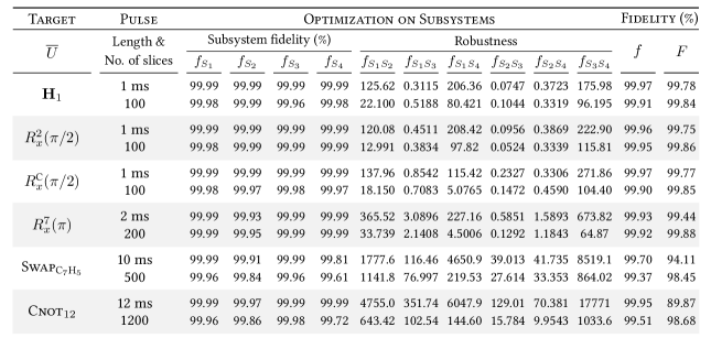
Figure 4: Shaped pulse optimized by our subsystem-based QOC method. For each target operation, we start from a random pulse guess, first optimize its subsystem fidelities with only considering intra-subsystem Hamiltonian $H_{0}$, and then optimize its robustness to inter-subsystem Hamiltonian $H_{1}$. In each row, the upper data mean pulse fidelities and robustness before the stage of robustness optimization, and the lower data mean pulse fidelities and robustness after the stage of robustness optimization.

References

- Brif et al. (2010) C. Brif, R. Chakrabarti, and H. Rabitz, Control of quantum phenomena: past, present and future, New J. Phys. 12, 075008 (2010).
- Letokhov (2007) V. Letokhov, Laser Control of Atoms and Molecules (Oxford University Press, Oxford, 2007).
- D’Alessandro (2008) D. D’Alessandro, Introduction to Quantum Control and Dynamics (Chapman & Hall, London, 2008).
- Dong and Petersen (2010) D. Dong and I. R. Petersen, Quantum control theory and applications: A survey, IET Control Theory Appl. 4, 2651 (2010).
- Acín et al. (2018) A. Acín, I. Bloch, H. Buhrman, T. Calarco, C. Eichler, J. Eisert, D. Esteve, N. Gisin, S. J. Glaser, F. Jelezko, S. Kuhr, M. Lewenstein, M. F. Riedel, P. O. Schmidt, R. Thew, A. Wallraff, I. Walmsley, and F. K. Wilhelm, The quantum technologies roadmap: a European community view, New J. Phys. 20, 080201 (2018).
- Khaneja et al. (2005) N. Khaneja, T. Reiss, C. Kehlet, T. Schulte-Herbrüggen, and S. J.Glaser, Optimal control of coupled spin dynamics: design of NMR pulse sequences by gradient ascent algorithms, J. Magn. Reson. 172, 296 (2005).
- Hogben et al. (2011) H. Hogben, M. Krzystyniak, G. Charnock, P. Hore, and I. Kuprov, Spinach – A software library for simulation of spin dynamics in large spin systems, J. Magn. Reson. 208, 179 (2011).
- Dolde et al. (2014) F. Dolde, V. Bergholm, Y. Wang, I. Jakobi, B. Naydenov, S. Pezzagna, J. Meijer, F. Jelezko, P. Neumann, T. Schulte-Herbrüggen, J. Biamonte, and J. Wrachtrup, High-fidelity spin entanglement using optimal control, Nat. Commun. 5, 3371 (2014).
- Geng et al. (2016) J. Geng, Y. Wu, X. Wang, K. Xu, F. Shi, Y. Xie, X. Rong, and J. Du, Experimental Time-Optimal Universal Control of Spin Qubits in Solids, Phys. Rev. Lett. 117, 170501 (2016).
- Rosi et al. (2013) S. Rosi, A. Bernard, N. Fabbri, L. Fallani, C. Fort, M. Inguscio, T. Calarco, and S. Montangero, Fast closed-loop optimal control of ultracold atoms in an optical lattice, Phys. Rev. A 88, 021601 (2013).
- Kelly et al. (2014) J. Kelly, R. Barends, B. Campbell, Y. Chen, Z. Chen, B. Chiaro, A. Dunsworth, A. G. Fowler, I.-C. Hoi, E. Jeffrey, A. Megrant, J. Mutus, C. Neill, P. J. J. O’Malley, C. Quintana, P. Roushan, D. Sank, A. Vainsencher, J. Wenner, T. C. White, A. N. Cleland, and J. M. Martinis, Optimal Quantum Control Using Randomized Benchmarking, Phys. Rev. Lett. 112, 240504 (2014).
- Zahedinejad et al. (2015) E. Zahedinejad, J. Ghosh, and B. C. Sanders, High-fidelity single-shot toffoli gate via quantum control, Phys. Rev. Lett. 114, 200502 (2015).
- Machnes et al. (2018) S. Machnes, E. Assémat, D. Tannor, and F. K. Wilhelm, Tunable, Flexible, and Efficient Optimization of Control Pulses for Practical Qubits, Phys. Rev. Lett. 120, 150401 (2018).
- Choi et al. (2014) T. Choi, S. Debnath, T. A. Manning, C. Figgatt, Z.-X. Gong, L.-M. Duan, and C. Monroe, Optimal Quantum Control of Multimode Couplings between Trapped Ion Qubits for Scalable Entanglement, Phys. Rev. Lett. 112, 190502 (2014).
- Lloyd and Montangero (2014) S. Lloyd and S. Montangero, Information Theoretical Analysis of Quantum Optimal Control, Phys. Rev. Lett. 113, 010502 (2014).
- Egger and Wilhelm (2014) D. J. Egger and F. K. Wilhelm, Adaptive Hybrid Optimal Quantum Control for Imprecisely Characterized Systems, Phys. Rev. Lett. 112, 240503 (2014).
- Day et al. (2019) A. G. R. Day, M. Bukov, P. Weinberg, P. Mehta, and D. Sels, Glassy Phase of Optimal Quantum Control, Phys. Rev. Lett. 122, 020601 (2019).
- Borzì et al. (2017) A. Borzì, G. Ciaramella, and M. Sprengel, Formulation and Numerical Solution of Quantum Control Problems (Society for Industrial and Applied Mathematics, 2017).
- Khaneja et al. (2001) N. Khaneja, R. Brockett, and S. J. Glaser, Time optimal control in spin systems, Phys. Rev. A 63, 032308 (2001).
- Khaneja et al. (2002) N. Khaneja, S. J. Glaser, and R. Brockett, Sub-Riemannian geometry and time optimal control of three spin systems: Quantum gates and coherence transfer, Phys. Rev. A 65, 032301 (2002).
- Lapert et al. (2010) M. Lapert, Y. Zhang, M. Braun, S. J. Glaser, and D. Sugny, Singular Extremals for the Time-Optimal Control of Dissipative Spin Particles, Phys. Rev. Lett. 104, 083001 (2010).
- Bukov et al. (2018) M. Bukov, A. G. R. Day, D. Sels, P. Weinberg, A. Polkovnikov, and P. Mehta, Reinforcement learning in different phases of quantum control, Phys. Rev. X 8, 031086 (2018).
- Doria et al. (2011) P. Doria, T. Calarco, and S. Montangero, Optimal Control Technique for Many-Body Quantum Dynamics, Phys. Rev. Lett. 106, 190501 (2011).
- (24) A. Ma, A. B. Magann, T.-S. Ho, and H. Rabitz, Optimal control of interacting quantum systems based on the first-order Magnus approximation: Application to multiple dipole-dipole coupled molecular rotors, arXiv:1811.12785 [quant-ph] .
- Li et al. (2017) J. Li, X. Yang, X. Peng, and C.-P. Sun, Hybrid Quantum-Classical Approach to Quantum Optimal Control, Phys. Rev. Lett. 118, 150503 (2017).
- Lu et al. (2017) D. Lu, K. Li, J. Li, H. Katiyar, A. J. Park, G. Feng, T. Xin, H. Li, G. Long, A. Brodutch, J. Baugh, B. Zeng, and R. Laflamme, Enhancing quantum control by bootstrapping a quantum processor of 12 qubits, npj Quantum Inf. 3, 45 (2017).
- Ryan et al. (2008) C. A. Ryan, C. Negrevergne, M. Laforest, E. Knill, and R. Laflamme, Liquid-state nuclear magnetic resonance as a testbed for developing quantum control methods, Phys. Rev. A 78, 012328 (2008).
- (28) H. Haas, D. Puzzuoli, F. Zhang, and D. G. Cory, Engineering Effective Hamiltonians, arXiv:1904.02702v1 .
- Dyson (1949) F. J. Dyson, The Radiation Theories of Tomonaga, Schwinger, and Feynman, Phys. Rev. 75, 486 (1949).
- (30) See Supplemental Material for more details.
- Loan (1978) C. V. Loan, Computing integrals involving the matrix exponential, IEEE Trans. Automat. Contr. 23, 395 (1978).
- Carbonell et al. (2008) F. Carbonell, J. C. Jímenez, and L. M. Pedroso, Computing multiple integrals involving matrix exponentials, J Comput. Appl. Math. 213, 300 (2008).
- Elliott (2009) D. Elliott, Bilinear Control Systems: Matrices in Action (Springer, New York, 2009).
- Li et al. (2019) J. Li, Z. Luo, T. Xin, H. Wang, D. Kribs, D. Lu, B. Zeng, and R. Laflamme, Experimental Implementation of Efficient Quantum Pseudorandomness on a 12-Spin System, Phys. Rev. Lett. 123, 030502 (2019).
- Debnath et al. (2016) S. Debnath, N. M. Linke, C. Figgatt, K. A. Landsman, K. Wright, and C. Monroe, Demonstration of a small programmable quantum computer with atomic qubits, Nature 536, 63 (2016).
- Preskill (2018) J. Preskill, Quantum Computing in the NISQ era and beyond, Quantum 2, 79 (2018).
- Poggiali et al. (2018) F. Poggiali, P. Cappellaro, and N. Fabbri, Optimal Control for One-Qubit Quantum Sensing, Phys. Rev. X 8, 021059 (2018).