Calibration and Performance of the NIKA2 camera at the IRAM 30-meter Telescope

Abstract

Context. NIKA2 is a dual-band millimetre continuum camera of 2 900 Kinetic Inductance Detectors (KID), operating at $150$ and $260\,\rm{GHz}$, installed at the IRAM 30-meter telescope in Spain. Open to the scientific community since October 2017, NIKA2 will provide key observations for the next decade to address a wide range of open questions in astrophysics and cosmology.

Aims. We present the calibration method and the performance assessment of NIKA2 after one year of observation.

Methods. We use a large data set acquired between January 2017 and February 2018 including observations of primary and secondary calibrators and faint sources that span the whole range of observing elevations and atmospheric conditions encountered at the IRAM 30-m telescope. This allows us to test the stability of the performance parameters against time evolution and observing conditions. We describe a standard calibration method, referred to as the baseline method, to go from raw data to flux density measurements. This includes the determination of the detector positions in the sky, the selection of the detectors, the measurement of the beam pattern, the estimation of the atmospheric opacity, the calibration of absolute flux-density scale, the flat fielding, and the photometry. We assess the robustness of the performance results using the baseline method against systematic effects by comparing to results using alternative methods.

Results. We report an instantaneous field of view (FOV) of 6.5’ in diameter, filled with an average fraction of $84\%$ and $90\%$ of valid detectors at $150$ and $260\,\rm{GHz}$, respectively. The beam pattern is characterized by a FWHM of $17.6^{\prime\prime}\pm 0.1^{\prime\prime}$ and $11.1^{\prime\prime}\pm 0.2^{\prime\prime}$, and a main beam efficiency of $47\%\pm 3\%$ and $64\%\pm 3\%$ at $150$ and $260\,\rm{GHz}$, respectively. The point-source rms calibration uncertainties are about $3\%$ at $150\,\rm{GHz}$ and $6\%$ at $260\,\rm{GHz}$. This demonstrates the accuracy of the methods that we have deployed to correct for atmospheric attenuation. The absolute calibration uncertainties are of $5\%$ and the systematic calibration uncertainties evaluated at the IRAM 30-$\rm{m}$ reference Winter observing conditions are below $1\%$ in both channels. The noise equivalent flux density (NEFD) at $150$ and $260\,\rm{GHz}$ are of $9\pm 1\,\rm{mJy}\cdot s^{1/2}$ and $30\pm 3\,\rm{mJy}\cdot s^{1/2}$. This state-of-the-art performance confers NIKA2 with mapping speeds of $1388\pm 174$ and $111\pm 11\,\rm{arcmin}^{2}\cdot\rm{mJy}^{-2}\cdot\rm{h}^{-1}$ at $150$ and $260\,\rm{GHz}$.

Conclusions. With these unique capabilities of fast dual-band mapping at high (better that 18”) angular resolution, NIKA2 is providing an unprecedented view of the millimetre Universe.

1 Introduction

Sub-millimetre and millimetre domains offer a unique view of the Universe from nearby astrophysical objects, including planets, planetary systems, galactic sources, nearby galaxies, to high-redshift cosmological probes, e.g. distant dusty star-forming galaxies, clusters of galaxies, Cosmic Infrared Background (CIB), Cosmic Microwave Background (CMB).

Ground-based continuum millimetre experiments have made spectacular progress in the past-two decades thanks to the advent of large arrays of high-sensitivity detectors (Wilson et al., 2008; Siringo et al., 2009; Staguhn et al., 2011; Swetz et al., 2011; Monfardini et al., 2011; Arnold et al., 2012; Bleem et al., 2012; Holland et al., 2013; Dicker et al., 2014; BICEP2 Collaboration et al., 2015; Adam et al., 2017a; Kang et al., 2018). This fast growth will continue as experimental efforts are driven by two challenges: improving the sensitivity to the polarisation to detect the signature of the end-of-inflation gravitational waves in the CMB, and improving the angular resolution. The latter has several important scientific implications: reaching arcminute angular resolution to exploit the CMB secondary anisotropies as cosmological probes, and sub-arcminute resolution to unveil the inner structure of faint or complex astrophysical objects and to map the early universe down to the confusion limit. Furthermore, new generation of sub-arcminute millimetre experiments, like NIKA2, which combines high angular resolution with a high mapping speed and a large coverage in the frequency domain, will achieve a breakthrough in our detailed understanding of the formation and evolution of structures throughout the Universe.

The New IRAM KID Array Two, NIKA2, is a sub-arcminute-resolution high-mapping speed camera observing simultaneously a 6.5’ diameter field of view (FOV) in intensity in two frequency channels centred at 150 and $260\,\rm{GHz}$ and in polarisation at $260\,\rm{GHz}$ (Adam et al., 2018). NIKA2 was installed at the IRAM 30-$\rm{m}$ telescope in October 2015 with a partial readout electronics, and operated in the final instrumental configuration since January 2017. After a successful commissioning phase that ended in October 2017, NIKA2 is open to the community for science-purpose observations for the next decade. NIKA2 will provide key observations both at the galactic scale and at high redshifts to address a plethora of open questions, including the environment impact on dust properties, the star formation processes at low and high redshifts, the evolution of the large-scale structures and the exploitation of galaxy clusters for accurate cosmology.

At the galactic scale, progress in understanding the star formation process relates to an accurate characterization of dust properties in the interstellar medium (ISM). NIKA2 will provide the high-resolution high-mapping speed dual-wavelength millimetre observations that are required for the determination of the mass and emissivity of statistically significant samples of dense, cold, star-forming molecular clouds (Rigby et al., 2018). Deep multi-wavelengths surveys of nearby galaxies and of large areas of the galactic plane also allows for setting constraints on environmental-related variations of the dust properties. Furthermore, NIKA2 observations are needed for a detailed study of the inner molecular cloud filamentary structure that hosts Solar-mass star progenitors (Bracco et al., 2017), to understand the evolution process that culminates in star formation (see e.g. André et al. (2014) for a review). Ultimately, these observations are also helpful to understand planet formation within proto-planetary disks.

For cosmology, NIKA2 observations will have two major implications. On the one hand, they represent a unique opportunity to study the evolution of the galaxy cluster mass calibration with redshift and dynamical state for their accurate exploitation as cosmological probe. Galaxy clusters are efficiently detected via the thermal Sunyaev-Zel’dovich (tSZ) effect (Sunyaev & Zeldovich, 1970) up to high redshifts ($z<1.5$), as was recently proven by CMB experiments (Hasselfield et al., 2013; Reichardt et al., 2013; Ade et al., 2016a). The exploitation of the vast SZ-selected galaxy cluster catalogues is currently the most powerful approach for cosmology with galaxy clusters (Ade et al., 2016b). However, the accuracy of the tSZ cluster cosmology relies on the calibration of the relation between the tSZ observable and the cluster mass and on the assessment of both its redshift evolution and the impact of the complex cluster physics on its calibration. Previous arcminute resolution experiments only allowed detailed studies of the intra cluster medium spatial distribution for low redshift clusters (z ¡ 0.2). Sub-arcminute resolution high mapping speed experiments are required to extend our understanding of galaxy cluster towards high redshift (Mroczkowski et al., 2019). The first high-resolution tSZ mapping of a galaxy cluster with NIKA2 has been reported in Ruppin et al. (2018). Furthermore, NIKA2 capabilities for the characterization of high-redshift ($0.5<z<0.9$) galaxy clusters have been verified using numerical simulation (Ruppin et al., 2019b), and their implication for cosmology has been discussed in Ruppin et al. (2019a).

On the other hand, in-depth mapping of large extragalactic fields with sub-arcminute resolution with NIKA2 will provide unprecedented insight on the distant universe. Indeed, the high-angular resolution of NIKA2 is key to reduce the confusion noise, which is the ultimate limit of single-dish cosmological surveys (Bethermin et al., 2017), and the high mapping speed allows to cover large area. This unique combination will result in detecting hundreds of dust-obscured optically-faint galaxies up very high redshift ($z\sim 6$) during their major episodes of star formation. This will help quantifying the star formation up to $z\sim 6$. Note that galaxy redshifts will have to be obtained with spectroscopic follow-up observations (e.g. with NOEMA) or multi-wavelength spectral energy distribution fittings (e.g. in the GOODS-N field thanks to the tremendous amount of ancillary data). Galaxy formation studies will also benefit from the large instantaneous field-of-view, high-resolution observations of NIKA2.

Indeed, hundreds of dust-obscured optically-faint galaxies will be detected up to very high redshift ($z\sim 6$) during their major episodes of star formation. The high-angular resolution of NIKA2 is key to reduce the confusion noise, which is the ultimate limit of single-dish cosmological surveys (Bethermin et al., 2017), and the high mapping speed allows to cover large area. This unique combination will help quantifying the star formation history up to $z\sim 6$. Note that galaxy redshifts will have to be obtained with spectroscopic follow-up observations (e.g. with NOEMA) or multi-wavelength spectral energy distribution fittings (e.g. in the GOODS-N field thanks to the tremendous amount of ancillary data).

The current generation of sub-arcminute resolution experiments also include the Large APEX Bolometer Camera (LABOCA (Siringo et al., 2009)) at the Atacama Pathfinder Experiment (APEX) 12-meter telescope, which covers a 12’ diameter FOV at $345\,\rm{GHz}$ at an angular resolution of about 19”; AzTEC at the 50-meter Large Millimeter Telescope, which operates with a single bandpass centred at either 143, 217 or $270\,\rm{GHz}$ (Wilson et al., 2008), and which has a beam FWHM of 5, 10 or $18^{\prime\prime}$, respectively; the Submillimeter Common User Bolometer Array Two (SCUBA-2 (Holland et al., 2013; Dempsey et al., 2013)) on the 15-meter James Clerk Maxwell Telescope, which simultaneously images a FOV of about 7’ at $353\,\rm{GHz}$ and $666\,\rm{GHz}$ with a main beam FWHM of 13” and 8” in the two frequency channels, respectively ; MUSTANG-2 at the 100-meter Green Bank telescope, which maps a 4.35’ FOV at $90\,\rm{GHz}$ with 9” resolution (Dicker et al., 2014; Stanchfield et al., 2016). Therefore, NIKA2 is unique in combining an angular resolution better than 20”, an instantaneous FOV of a diameter of 6.5’ and multi-band observation capabilities at $150$ and $260\,\rm{GHz}$.

Most of the other millimetre instruments consist of bolometric cameras. By contrast, NIKA2 is based on the Kinetic Inductance Detectors (KID) technology (Day et al., 2003; Doyle et al., 2008; Shu et al., 2018). This concept has been first demonstrated with a pathfinder instrument, NIKA (Monfardini et al., 2010, 2011). Installed at the IRAM 30-m telescope until 2015, NIKA demonstrated state-of-the-art performance (Catalano et al., 2014), and obtained breakthrough results (see e.g., Adam et al. (2014, 2017b). NIKA has been crucial in optimizing the NIKA2 instrument and data analysis.

A thorough description of the NIKA2 instrument is presented in Adam et al. (2018), along with the results of the commissioning in intensity based on the data acquired during the two technical campaigns of 2017. In the present paper, we propose a standard calibration method, which is referred to as the baseline calibration, to go from raw data to stable and accurate flux density measurements. amount of data acquired between January 2017 and February 2018. Regarding the performance of the polarization capabilities, their assessment will be addressed in a forthcoming paper. To achieve a reliable and high-accuracy estimation of the performance, we perform extensive testing of the stability with respect to both the analysis methodological choices and to the observing conditions. First, the methodological choices and hypothesis may have an impact on the performance results and the systematic errors. At each step of the calibration procedure and for each performance metrics, we compare the results obtained using the baseline method to alternative approaches to ensure the robustness against systematic effects. Second, we check the stability of the results using a large number of independent data sets corresponding to various observing conditions. Specifically, most of the performance assessment relies on data acquired during the February 2017 technical campaign (N2R9) and the October 2017 (N2R12) and January 2018 (N2R14) first and second scientific-purpose observation campaigns. These observation campaigns are referred to as the reference observation campaigns. Each campaign consists of about 1300 observation scans lasting between two and twenty minutes for a total observation time of about 150 hours.

This paper constitutes a review of NIKA2 calibration and performance assessment in intensity. It is intended to be a reference for observations with NIKA2, which will last at least for ten years. The outline of the paper is as follows: Sect. 2 to 4 give short summaries of the instrumental set up, the observational modes and the data analysis methods that have been used for the calibration and the performance assessment. Sect. 5 to 10 detail the dedicated calibration methods, extract the key characteristic results and discuss their accuracy and robustness. The field-of-view reconstruction and the KID selection for science purpose are discussed in Sect. 5. The beam pattern is characterized in Sect. 6, along with the main beam full-width at half maximum and the beam efficiency. Sect. 7 is dedicated to the derivation of the atmospheric opacity. The methods that we have proposed to calibrate are gathered in Sect. 8, while Sect. 9 presents the validation of these methods and the calibration accuracy and stability assessment. The noise characteristics and the sensitivity are discussed in Sect. 10. Finally, Sect. 11 summarizes the main measured performance characteristics and briefly describes next steps for future improvements on NIKA2.

2 General view of the instrument

NIKA2 simultaneously images a FOV of 6.5’ in diameter at 150 and $260\,\rm{GHz}$. It also has polarimetry capabilities at $260\,\rm{GHz}$, which are not discussed here. To cover the 6.5’-diameter FOV without degrading the telescope angular resolution, NIKA2 employs a total of around 2 900 KIDs split over three distinct arrays, one for the $150\,\rm{GHz}$ band and two for the $260\,\rm{GHz}$ band.

A detailed description of the instrument can be found in Adam et al. (2018) and Calvo et al. (2016). We briefly present here the main sub-systems focusing on the elements that are specific to NIKA2 or that drive the development of dedicated procedures for the data reduction or calibration.

2.1 Cryogenics

KIDs are superconducting detectors, which in the case of NIKA2 are made of thin-aluminium films deposited on a silicon substrate (Roesch et al., 2012). For an optimal sensitivity, they must operate at a temperature of around 150 mK, that is roughly one order of magnitude lower than the aluminium superconducting transition temperature. For this reason, NIKA2 employs a custom-built dilution fridge to cool down the focal plane, and the refractive elements of the optics. Overall, a total mass of around $100\,\rm{kg}$ is kept deeply in the sub-Kelvin regime. Despite the complexity and huge size of the system, the operation of NIKA2 does not require external cryogenic liquids and can be fully operated remotely.

2.2 Optics

The NIKA2 camera optics include two cold mirrors and six lenses. The filtering of unwanted (off-band) radiation is provided by a suitable stack of multi-mesh filters as thermal blockers placed at all temperature stages between 150 mK and room temperature. Two aperture stops, at a temperature of 150 mK, are conservatively designed to limit the entrance pupil of the optical system to the inner 27.5 m diameter of the primary mirror. An air-gap dichroic plate splits the 150 GHz (reflection) from the 260 GHz (transmission) beams. This element, which is made of a series of thin micron-like membranes separated by calibrated rings and mounted on a native ring in stainless steel, has been designed to resist to low temperature-induced deformation. As discussed in Sect. 8.2, the air-gap technology has been proven to be efficient in preserving the planarity of the dichroic, but shows sub-optimal performance in transmission. Moreover, a grid polariser ensures the separation of the vertical and horizontal components of the linear polarizations on the 260 GHz channel. Band-defining filters, custom-designed to optimally match the atmospheric windows while ensuring robustness against average atmospheric condition at 260 GHz, are installed in front of each array. A half-wave polarization modulator is added at room temperature when operating the instrument in polarimetry mode.

Hereafter, the detector array illuminated by the 150 GHz ($2\,\rm{mm}$) beam is named Array 2 (A2), while in the 260 GHz ($1.15\,\rm{mm}$) channel, the array mapping the horizontal component of the polarization is referred to as Array 1 (A1) and the one mapping the vertical component is called Array 3 (A3). The 150 GHz observing channel is referred to as the $2\,\rm{mm}$ band and the 260 GHz channel as the $1\,\rm{mm}$ band.

2.3 KIDs and electronics

Array 2 consists of 616 KIDs, arranged to cover a 78 mm diameter circle. Each pixel has a size of $2.8\times 2.8\textrm{\,mm}^{2}$, which is the maximum pixel size allowed not to degrade the theoretical 30-$\rm{m}$ telescope angular resolution. In the case of the 260 GHz band detectors, the pixel size is $2\times 2\mathrm{\,mm}^{2}$, to ensure a comparable sampling of the focal plane. This results in a sampling slightly above $\lambda/D$ in this channel, where $D$ is the diameter aperture, as discussed in Sect. 5.2. In order to ensure a full coverage of the 6.5’ FOV, a total of 1,140 pixels is needed in each of the two 260 GHz arrays A1 and A3.

The key advantage of the KID technology is the simplicity of the cold electronics and the multiplexing scheme. In NIKA2, each block of around 150 detectors is connected to single coaxial line linked to the readout electronics (Bourrion et al., 2016). Hence Array 2 is connected to four different readout feed-lines, while Array 1$\&$3 are both equipped with eight feed-lines. The warm electronics required to digitize and process the pixels signals is composed of twenty custom-built readout cards (one per feed-line).

2.4 KID photometry and tuning

KIDs are superconducting resonators whose resonance frequency shift linearly depends on the incoming optical power. This was theoretically demonstrated in Swenson et al. (2010) and confirmed for NIKA KIDs, which have a similar design to the current NIKA2 KIDs, using laboratory measurements, as discussed in Monfardini et al. (2014). The measurement of the KID frequency shift $\Delta f$ is critical for the use of KIDs as mm-wave detectors.

For the KID readout, an excitation signal is sent into the cryostat on the feed-line coupled to the KID. The excitation tones produced by the electronics are amplified by a cryogenic (4 K) low noise amplifier after passing through the KIDs and being analysed by the readout electronics. Each KID is thus associated with an excitation tone at a frequency $f_{\rm{tone}}$, which corresponds to an estimate of its resonance frequency for a reference background optical load. The transmitted signal can be described by its amplitude and phase, or, as is common practice for KID, by its $I$ (in-phase) and $Q$ (quadrature) components with respect to the excitation signal. The goal is now to relate the measured variations of the KID response to the excitation signal $(\Delta I,\Delta Q)$, which are induced by incident light, to $\Delta f$. For this, the electronics modulates the excitation tone frequency $f_{\rm{tone}}$ at about 1 kHz with a known frequency variation $\delta f$ and the read out gives the induced transmitted signal variations $(dI,dQ)$. Projecting linearly $(\Delta I,\Delta Q)$ on $(dI,dQ)$ therefore provides $\Delta f$. This quantity, in Hz, constitutes the raw KID time-ordered data, which are sampled at a frequency of $23.84\,\rm{Hz}$. For historical reasons, this way of deriving KID signals has been nicknamed RfdIdQ. More details on this process are given in Calvo et al. (2013). Once ingested into the calibration pipeline, the raw data will be further converted into astronomical units (Sect. 8).

In addition to light of astronomical origin, any change in the background optical load (due, for example, to changes in the atmospheric emission with elevation) contributes as well to the shift of the KID resonance frequencies. In order to maximize the sensitivity of a KID, the excitation signal $f_{\rm{tone}}$ must always be near the KID resonance frequency. We therefore have developed a tuning algorithm that performs this optimization. A tuning is performed at the beginning of each observation scan to adapt the KIDs $f_{\rm{tone}}$ to the working background conditions. This process takes only a few seconds. These optimal conditions are further maintained by performing continuous tunings between two scans while NIKA2 is not observing, to match regularly with the observing conditions.

2.5 Bandpasses

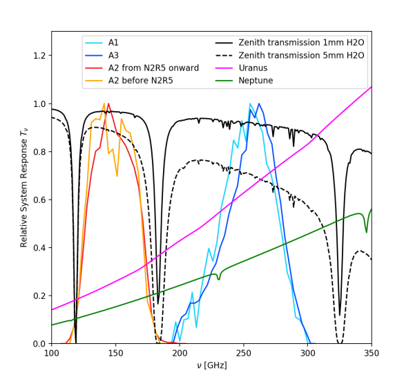
Figure 1: Relative system response of the three KID arrays as a function of frequency. For illustration we also show in black the atmospheric transmission obtained with the ATM model (Pety et al., 2009; Pardo et al., 2001) for two values of precipitable water vapour (1 and $5\,\rm{mm}$). The spectra of the model of Uranus (pink) and the model of Neptune (green), as discussed in Appendix A, are also plotted for illustration with arbitrary normalization with respect to the NIKA2 transmission.

The NIKA2 spectral bands have been measured in laboratory using a Martin-Puplett interferometer built in-house (Durand, 2007). The measurement relies on using the difference of two black body radiations used as input signal for the interferometer. Both arrays and filter bands were considered in the measurements, while the dichroic element was not included. Figure 1 shows the relative spectral response for the three arrays. Notice that Array 2 was upgraded in September 2016 (during the so-called N2R5 technical campaign) and that the spectral transmissions are slightly different (red and orange lines in Fig. 1).

The two arrays operating at 260 GHz, mapping different linear polarisations, exhibit a slightly different spectral behaviour as can be seen on Fig. 1. Besides the effect of the optical elements in front of the two arrays, this may be explained by a tiny difference in the silicon wafer, the difference of the Aluminium film thickness of the KID arrays and/or the different responses for two polarisations of the detector (Adam et al., 2018; Shu et al., 2018).

It is clear from Fig. 1 that the atmosphere will modify the overall transmission of the system, especially at the transmission tails for A2. To highlight this effect we compute an effective frequency $\nu_{\rm{eff}}$ computed as the weighted integral of the frequency considering the NIKA2 bandpass and the SED of Uranus, for various atmospheric conditions. In Table 1, we give $\nu_{\rm{eff}}$ and the bandwidths $\Delta\nu$ computed both at zero atmospheric opacity and for the reference IRAM 30-$\rm{m}$ winter-semester observing conditions (defined by an atmospheric content of $2\,\rm{mm}$ of precipitable water vapour and an observing elevation of $60^{o}$).

Table 1: Effective frequencies $\nu_{\rm{eff}}$ and bandwidths $\Delta\nu$ of the three arrays computed in two different observing conditions defined with the precipitable water vapour (pwv) contents in mm and the observing elevation in degrees).

	Array 1	Array 3	Array 2
$\nu_{\rm{eff}}$ (0mm, 90deg) [GHz]	254.7	257.4	150.9
$\Delta\nu$ (0mm, 90deg) [GHz]	49.2	48.0	40.7
$\nu_{\rm{eff}}$ (2mm, 60deg) [GHz]	254.2	257.1	150.6
$\Delta\nu$ (2mm, 60deg) [GHz]	48.7	47.9	39.2

In laboratory spectral characterization allows the bandpass of the three arrays to be measured with uncertainties better than one percent. The bandpass characterization will be further improved using in-situ measurements with a new Martin-Puplett interferometer designed to be placed in front of the cryostat window, which will allow to account for the whole optical system, including the dichroic plate. As it will be discussed in Sect. 8, the baseline calibration method only resorts to the bandpass measurements for color correction estimations in order to mitigate the bandpass uncertainty propagation in the flux density measurement. In fact, for each array, we define reference frequencies to define NIKA2 photometric system. These are 260 GHz for the A1 and A3 and 150 GHz for A2.

3 Observations

This section presents the different observation modes that are used at the IRAM 30-$\rm{m}$ telescope for both commissioning and scientific-purpose observations with NIKA2. Each observation campaign is organized as observing pool allowing to optimize observations of several science targets in a flexible way. Most of these observing scans are on-the-fly (OTF) raster scans, which consist of a series of scans at constant azimuth or elevation (right ascension or declination) and varying elevation or azimuth (declination or right ascension). Their characteristics have been tailored for NIKA2 performance.

3.1 Focus

Observation pools start with setting the telescope focus since NIKA2 large FOV alleviates the need to adjust the pointing beforehand. We have designed a specific focus procedure that takes advantage of the dense sampling of the FOV allowing to map a source in a short integration time. We perform a series of five successive one-minute raster scans of a bright (above a few Jy) point source at five axial offsets of the secondary mirror (M2) along the optical axis. As the scan size is $1^{\prime}\times 5^{\prime}$, the main contribution to each map mainly comes from the KIDs located in the central part of the FOV.

Elliptical Gaussian fits on the five maps provide estimates of the flux and FWHM along minor and major axes for each focus. The best axial focus in the central part of the array is then estimated as the maximum of the flux or the minimum of the FWHM using parabolic fits of the five measurements.

As presented in more details in Appendix B, the focus surface, that is defined as the locations of the best focus across the whole FOV is not flat but rather slightly bowl-shaped. To account for the curvature of the focus surfaces and optimize the average focus across the FOV, we add -0.2 mm to the best axial focus in the central part of the array. This focus offset is measured on data using a dedicated sequence of de-focused scans, as discussed in Appendix B. It is in agreement with expectations derived with optical simulation using ZEMAX.

Axial focus offsets are measured every other hour during daytime and are systematically checked after sunrises and sunsets, while one or two checks suffice during night. Lateral focus offsets can also be checked in a similar way, but are found to stay constant over periods of time that cover several observing campaigns.

3.2 Pointing

Once the instrument is correctly focused, we can estimate pointing corrections before scientific observations. Based on general operating experience at the 30-$\rm{m}$ telescope, we use the so-called pointing or cross-type scans to monitor the pointing during observations. The telescope executes a back and forth scan in azimuth and a back and forth scan in elevation, centred on the observed source. We fit Gaussian profiles from the timelines of the reference detector, which is chosen as a valid detector located close to the center of Array 2. The choice of a reference detector operated at $150\,\rm{GHz}$ is suitable since most of our pointing sources are radio sources. We use the estimated position of the reference detector to derive the current pointing offsets of the system in azimuth and elevation. This correction is propagated to the following scans. The pointing is monitored in an hourly basis.

In addition, we perform pointing sessions in order to refine NIKA2 pointing model. A pointing session consists in observing about 30 sources on a wide range of elevations and azimuth angles while monitoring the pointing offsets that are measured for each observation. During N2R9 technical campaign, the rms of the residual scatter after pointing offset correction was $1.62^{\prime\prime}$ in azimuth and $1.37^{\prime\prime}$ in elevation. We conservatively report rms pointing errors $<3^{\prime\prime}$.

3.3 Skydip

A skydip scan consists in a step-by-step sky scan along a large range of elevations. NIKA2 skydips are not used for the scan-to-scan atmospheric calibration. For this purpose, the KIDs are used as total power detectors to estimate the emission of the atmosphere and hence, the atmospheric opacity, as discussed in Sect. 7. NIKA2 skydips therefore serve to calibrate the KID responses with respect to the atmospheric background for atmospheric opacity derivation.

Unlike heterodyne receivers for which skydips can be conducted continuously slewing the telescope in elevation, the NIKA2 camera cannot resort to such method, as the KIDs need to be retuned for a given air mass. A NIKA2 skydip, which is quoted skydip, comprises eleven steps in the elevation range from 19 to 65 degrees, regularly spaced in air mass. For each step, we acquire about twenty seconds of data to ensure a precise measurements. KIDs are tuned at the beginning of each constant elevation sub-scan (hence once per air mass).

Skydips are typically performed every eight hours for a wide spanning of the atmospheric conditions through an observation campaign.

3.4 Beam map

A beammap scan is a raster scan in ($\rm{az}$, $\rm{el}$) coordinates tailored to map a bright compact source, often a planet, with steps of 4.8”, that are small enough to ensure a half-beam sampling, which gives around 90% fidelity, for each KID. A scan of $13\times 7.8$ arcmin² is acquired either with the telescope performing a series of continuous slews at fixed elevation or at fixed azimuth. A continuous scanning slew defines a subscan. The fixed-elevation scanning has the advantage of suppressing the air-mass variation across a subscan, while the fixed-azimuth scanning offers an orthogonal scan direction to the former: the combination of both gives a more accurate determination of the far side lobes. The scan size is optimized to enable maps to be made for all KIDs, even those located at the edges of the array. Larger size in the scanning direction allows for correlated noise subtraction. During subscans, the telescope moves at 65 arcsec/s. The need to have high-fidelity sampling of 11” beams along the scan direction translates into a maximum speed of 97 arcsec/s, which ensures to have 2.7 samples per beam, for our nominal acquisition rate of 23.8 Hz, and is thus met with margins. For the sake of scanning efficiency with the 30-$\rm{m}$ telescope, the minimal duration for subscans is 10 s. For beammap scans, subscans last 12 s and the entire scan lasts about 25 min.

Beammaps are key observations for the calibration. Whereas a single beammap acquired in stable observing conditions could suffice, beammap scans are performed on a daily basis. More details on these observations are given in Sect. 5 where we describe how to actually exploit them to derive individual KID properties.

4 Data Reduction: from raw data to flux density maps

The raw KID data ($I$, $Q$, $\Delta I$, $\Delta Q$) and the telescope source-tracking data are synchronized by the NIKA2 acquisition system using a clock that gives the absolute astronomical time, that is the telescope pulses per second, to define the NIKA2 raw data. From the KID raw data, we compute a quantity that is proportional to the KID frequency shift using the RfdIdQ method, as described in Sect. 2.4. This quantity, which is hence proportional to the input signal, constitutes the KID time-ordered information (TOI).

We have developed a dedicated data reduction pipeline to produce calibrated sky maps from NIKA2 raw data. This pipeline was first developed for the data analysis during the commissioning campaigns and is currently used for science-purpose data reduction. The calibration and performance assessment relies on this pipeline. A detailed description of this software will be presented in a companion paper (Ponthieu et al., 2020), as well as an application to blind source detection. Here we summarize the main steps of the data reduction. Moreover, we focus the discussion on the treatment of point-like or compact sources, which are used for the performance assessment.

4.1 Low level processing

We isolate the relevant fraction of the data for scientific utilisation and we mask KIDs that do not meet the selection criteria, as discussed in Sect. 5.3, or timeline accidents (glitches). Specifically, we flag out cosmic rays, which impact only one data sample per hit due to the KID fast time constant (Catalano et al., 2014), and the KIDs for which the noise level exceed $3\sigma$ of the average noise level of all other KIDs of the same array.

4.2 Pointing reconstruction

We produce a timeline of the pointing positions of each KID with respect to the targeted source position (usually located at the center of the scan) using two sets of information. First, the control system of the telescope provides us with the absolute pointing of a reference point of the focal point, which is coincident with the reference KID after the pointing correction are applied, as described in Sect. 3.2. Second, we estimate the offset positions of each KID with respect to the reference KID using a dedicated procedure that is referred to as the focal plane reconstruction, as presented in Sect. 5. After this step, we are able to distinguish KIDs that are on-source from those that are off-source, which is a key information for dealing with the correlated noise.

4.3 TOI calibration

The KID TOI in units of Hz (frequency shifts) are converted to Jy/beam in two steps. First, the KID data are inter-calibrated using the calibration coefficients, a. k. a. relative gains, as discussed in Sect. 8.2 and the absolute scale of the flux density is set using the absolute calibration method discussed in Sect. 8.1. Second, the instantaneous line-of-sight atmospheric attenuation $\rm{exp}[{-\tau_{\nu}x(t)}]$ is corrected using the zenith opacity at the observing frequency $\nu$ $\tau_{\nu}$, which is estimated for a given scan as discussed in Sect. 7, and the instantaneous air mass $x(t)$. The latter is estimated as $(\sin\rm{el}_{t})^{-1}$ using the observing elevation $\rm{el}_{t}$, as obtained using the pointing reconstruction.

4.4 Correlated noise subtraction

The TOI of each KID include a prominent low-frequency component of correlated noise of two different origins: the atmospheric component, which is dominant with some rare exceptions and common to all KIDs, and the electronic noise, which is common to the KIDs connected to a same electronic readout feed-line (see Sect. 2.3). The subtraction of this correlated noise is a key step of the data processing, as correlated noise residuals are an important limiting factor of the sensitivity. We have devised several dedicated methods for this purpose. This will be thoroughly discussed in Ponthieu et al. (2020), whereas here we illustrate the general principle and only discuss the method routinely used for the calibration.

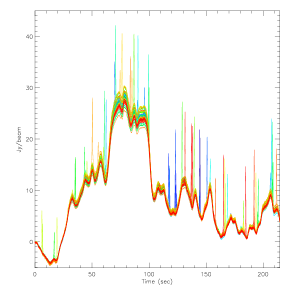
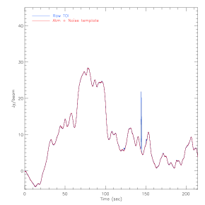
Figure 2: Example of variations of KID time-ordered information. Top: Example of 40 KID calibrated TOIs during an observation of Uranus. The low frequency correlated component (atmospheric and electronic noises) is clearly seen. Bottom: One of these TOIs (in blue) and the common mode that is subtracted from it (in red). The zero level is arbitrary.

As illustrated on the upper panel of Fig. 2, the low-frequency noise component is seen by all KIDs at the same time, while the astrophysical signal (Uranus in this case) is shifted from one KID to another. In this figure the KID TOIs have been rescaled to be null at $t=0$. A simple average of the KID TOIs provides an estimate of the low-frequency noise component, that we referred to as a common mode, while the signal is averaged out. The common mode shown as a red line on the lower panel of Fig. 2, is then subtracted to each KID TOI.

\begin{overpic}[clip={true},trim=14.22636pt 0.0pt 0.0pt 14.22636pt,width=173.44534pt]{Figures/pws_TOI_array_1_20170228s151_mod.pdf} \put(2.0,15.0){\rotatebox{90.0}{\scriptsize P${}_{\nu}$ [arbitrary units]}} \end{overpic}

\begin{overpic}[clip={true},trim=14.22636pt 0.0pt 0.0pt 14.22636pt,width=173.44534pt]{Figures/pws_TOI_array_3_20170228s151_mod.pdf} \put(2.0,15.0){\rotatebox{90.0}{\scriptsize P${}_{\nu}$ [arbitrary units]}} \end{overpic}

\begin{overpic}[clip={true},trim=14.22636pt 0.0pt 0.0pt 14.22636pt,width=173.44534pt]{Figures/pws_TOI_array_2_20170228s151_mod.pdf} \put(2.0,15.0){\rotatebox{90.0}{\scriptsize P${}_{\nu}$ [arbitrary units]}} \end{overpic}

Figure 3: The data noise power spectra are shown for the three NIKA2 arrays (A1, A3, and A2 from top to bottom). The power spectra are given for the raw data (blue), and for noise decorrelated data using the common mode (labelled CM, green), the PCA (red) and the Most Correlated Pixels (labelled MCP, cyan) methods.

For the calibration and performance assessment, we use an atmospheric and electronic noise decorrelation method named Most Correlated Pixels  which comprises two additional technicalities with respect to the common mode method. First, the signal contamination of the common mode estimate is mitigated by discarding on-source KID data samples before averaging the rescaled TOI. This is achieved by deriving a mask per TOI from the pointing information (Sect. 4.2), which is zero if the KID is close to the source, and equal to unity otherwise. In the case of a point source, the mask consists in a disk of a minimum radius of 60” centred on the source, whereas for diffuse emission, tailored masks driven by the source morphology are built using iterative methods, as for example in Ruppin et al. (2017). Second, instead of a single common mode subtraction to all KIDs, we estimate an accurate common mode for each KID. Calculating the KID-to-KID cross-correlation matrix, we identify the most correlated KIDs. Then, we build an inverse noise weighted co-addition of the timelines of the KIDs that are the most correlated with the KID under concern. Furthermore, we have tested on simulations that this method does preserves the flux of point-like or moderately extended sources.

Regarding diffuse emission, the noise decorrelation induces a filtering effect at large angular scales that must be corrected for to fully recover the large scale signal. A method to correct for the spatial filtering, which relies on the evaluation of the data processing transfer function using simulations, is described in Adam et al. (2015). The data processing transfer function depends on the morphological properties of the extended source under concern. An example of the data processing transfer function for NIKA2 observation towards a galaxy cluster is given in Ruppin et al. (2018), evidencing a prominent filtering at angular scales larger than the 6.5’ diameter FOV.

In Fig. 3 we present the noise power spectra of a typical KID TOI both before any data reduction and using three noise decorrelation methods, which are the simple common mode (CM) method used in Fig. 2, a method based on a principal component analysis (PCA) and the Most Correlated Pixels method (MCP). We observe that after decorrelation the $1/f$-like noise in the power spectra (principally due to atmospheric emission drifts) is significantly reduced leading to nearly flat spectra down to 0.5 Hz, with lower $1/f$-like residual noise for the PCA and the Most Correlated Pixels methods than the common mode decorrelation at low frequencies. The two former methods further subtract a substantial fraction of the correlated noise that originates from the electronic readouts. Moreover, we have checked using simulations that the Most Correlated Pixels method was more efficient than the PCA in preserving the astrophysical signal. The former is thus preferred over the latter.

4.5 Map projection

We use the pointing information to project the cleaned (low-frequency noise subtracted) calibrated TOI of all the valid KIDs of an array onto a flux density map (tangential projection). This map $M_{p}$ is produced using an inverse variance noise weighting of all of the data samples that fall into a map pixel as defined using a nearest grid point scheme. We also compute the associated count map $H_{p}$ defined as the number of data samples per map pixels. The map resolution is chosen small enough (typically $2^{\prime\prime}$ per map pixel) to alleviate the need for more refined interpolation scheme. The noise variance $\sigma_{k}$ for each KID $k$ is evaluated by the standard deviation of the KID TOI far from the source position. The variance map $\sigma_{p}^{2}$ is inhomogeneous and varies as the inverse of $H_{p}$. Its normalisation is evaluated using the homogeneous background map variance, that is the variance of $M_{p}\sqrt{H_{p}}$ calculated far from the source.

To account for the residual correlated noise while evaluating the variance map, we resort to an effective approach. First, we compute the map of the signal-to-noise ratio (SNR) as the ratio of $M_{p}$ and the noise map $\sigma_{p}$, that is the square root of the variance map. We observe that the distribution of the SNR map over the pixels far from the source is well-approximated with a Gaussian but has a width larger than the expected unity. This is due to the remaining correlations between KID TOIs before projection. Then, we multiply the noise map $\sigma_{p}$ by the required factor so that the width of SNR distribution becomes normalized. This normalizing factor ranges from 1.2 to 1.5 depending on the observing conditions. This constitutes an effective approach to account for the pixel-to-pixel correlation matrix off-diagonal terms alleviating the need of accurately measure them.

When several scans of the same source are averaged, we apply an inverse variance weighting as well. The variance map of the sum of scans is also corrected to ensure unity-width SNR distribution.

4.6 Observation scan selection

For calibration and performance assessment, we select scans in average observing conditions by performing mild selection cuts. These scan cuts rely on zenith opacity estimates $\tau_{\nu}$ in NIKA2 bands, as described in Sect. 7, on the elevation and on the observation time of the day. We select the scans satisfying the following criteria:

• $\tau_{\rm{A_{3}}}<0.5$, where $\tau_{\rm{A_{3}}}$ is the $\tau_{\nu}$ estimate for Array 3;

• $x\,\tau_{\rm{A_{3}}}<0.7$ and $\rm{el}>20^{o}$, where $\rm{el}$ is the observing elevation and $x$, the air mass, which depends on the elevation as $x=(\sin{\rm{el}})^{-1}$. This threshold corresponds to a decrease of the astrophysical signal by a factor of two;

• observation time from 22:00 to 9:00 UT and from 10:00 to 15:00 UT, that excludes the sunrise period and the late afternoon.

In the following sections, these selection cuts are referred to as the ’baseline scan selection’. As discussed in Sect. 8.3, the late afternoon observations are often affected by time-variable broadening of the telescope beams caused by (partial) solar irradiation of the primary mirror and/or anomalous atmospheric refraction. Around sunrise, the focus shifts continuously due to the ambient temperature change until the temperature stabilizes, so that the scans taken from 9:00 to 10:00 UT are likely not to be optimally focused. After the focus stabilisation, the middle of the day period ranging from 10:00 to 15:00 UT offers stable observing conditions provided that the telescope is not pointed too close to the Sun. Otherwise, further scan selection based on the exact sequence of observations and on beam monitoring might be needed before using these observations for performance assessment. In summary, the baseline scan selection retains 16 hours of observations a day and discards observations affected by an atmospheric absorption exceeding 100%.

5 Focal Plane Reconstruction

From the operational point-of-view the KIDs are defined by the resonance frequency and not by their physical position in the focal plane. Therefore, to find the position on the sky we need to deploy a dedicated method that we refer to as the FOV reconstruction. The FOV reconstruction thus consists in matching the KID frequency tones to positions in the sky and in performing a KID selection. Although all the 2,900 KID are responsive, some of them are affected by cross-talk or are noisy due to an inaccurate tuning of their frequency, and must be discarded for further analysis. We use beammaps, which enable an individual map per KID to be constructed to measure the KID positions and relative gains, as discussed in Sect. 5.1. The measured KID positions are further checked by matching with the design positions, as presented in Sect. 5.2. In Sect. 5.3, we present the final KID selection and FOV geometry, as obtained by repeating the procedure on a series of beammaps.

5.1 Reconstruction of the FOV positions and KID properties

In order to be able to produce a map, one needs to associate a pointing direction to any data sample of the system. The telescope provides pointing information for a reference position in the focal plane. These information consist of the absolute azimuth and elevation $(\rm{az}_{t}^{\rm{ref}},\rm{el}_{t}^{\rm{ref}})$ of the source, together with offsets $(\Delta\rm{az}_{t}^{\rm{ref}},\Delta\rm{el}_{t}^{\rm{ref}})$ w. r. t. these, which depends on the scanning strategy. We then need to know the relative pointing offsets of each detector with respect to this reference position. We use beammaps for this purpose (see Sect. 3.4).

We apply a median filter per KID timeline whose width is set to 31 samples, that is equivalent to about 5 FWHM at 65 arcsec/s and for the sampling frequency of 23.84 Hz. Then, we project one map per KID in Nasmyth coordinates. The median filter removes efficiently most of the low frequency atmospheric and electronic noise, albeit with a slight ringing and flux loss on the source. However, at this stage, we are only interested in the location of the observed source. To derive the Nasmyth coordinates from the provided $(\rm{az}_{t},\rm{el}_{t})$ and $(\Delta\rm{az}_{t},\Delta\rm{el}_{t})$ coordinates, we build the following quantities at time $t$:

$$\left({\begin{array}[]{c}\Delta x_{t}\\ \Delta y_{t}\\ \end{array}}\right)=\left({\begin{array}[]{cc}\cos\rm{el}_{t}&-\sin\rm{el}_{t}\\ \sin\rm{el}_{t}&\cos\rm{el}_{t}\\ \end{array}}\right)\left({\begin{array}[]{c}\Delta\rm{az}_{t}^{\rm{ref}}\\ \Delta\rm{el}_{t}^{\rm{ref}}\\ \end{array}}\right)$$ (1)

Note that $\Delta\rm{az}_{t}^{\rm{ref}}$ is already corrected by the $\cos\rm{el}_{t}^{\rm{ref}}$ factor to have orthonormal coordinates in the tangent plane of the sky and be immune to the geodesic convergence at the poles. The data timelines are then projected onto $(x,\,y)$ maps. We fit a 2D elliptical Gaussian on each KID Nasmyth map. The centroid position of this Gaussian provides us with an estimate of the KID pointing offsets w. r. t. the telescope reference position ($\rm{az}_{t}+\Delta\rm{az}_{t}$, $\rm{el}_{t}+\Delta\rm{el}_{t}$) in Nasmyth $(x,y)$ coordinates (independent of time).

To convert from Nasmyth offsets to $(\rm{az},\rm{el})$ offsets, we apply the following rotation:

$$\left({\begin{array}[]{c}\Delta\rm{az}^{k}_{t}\\ \Delta\rm{el}^{k}_{t}\\ \end{array}}\right)=\left({\begin{array}[]{cc}\cos\rm{el}_{t}&\sin\rm{el}_{t}\\ -\sin\rm{el}_{t}&\cos\rm{el}_{t}\\ \end{array}}\right)\left({\begin{array}[]{c}\Delta x^{k}\\ \Delta y^{k}\\ \end{array}}\right)$$ (2)

where $k$ is a KID index. Adding these offsets to $(\Delta\rm{az}_{t}^{\rm{ref}},\Delta\rm{el}_{t}^{\rm{ref}})$ gives the absolute pointing of each KID in these coordinates.

Furthermore, the fitted Gaussian per KID further provides us with a first estimate of the KID FWHM, ellipticity and sensitivity. We apply a first KID selection by removing outliers to the statistics on these parameters. We also discard manually KIDs that show a cross-talk counterpart on their map. We repeat this procedure using the baseline TOI decorrelation method instead of the median filter. Specifically, we apply the Most Correlated Pixels noise subtraction presented in Sect. 4 to the KID timelines, which are then used to produce maps per KID. Therefore this alleviates the flux loss induced by the median filter. This also ensures that the beammaps are treated in the same way as the scientific observation scans will. Finally, a second iteration of the KID selection is performed.

This analysis is repeated on all beammaps to obtain statistics and precision on each KID parameter, together with estimates on KID performance stability, as discussed in the next sections.

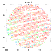
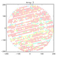
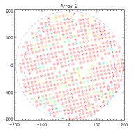
Figure 4: Average detector positions for arrays A1, A3, and A2. The three plots show the detectors that met the selection quality criteria for at least two beammaps during two technical campaigns. These consist of 952, 961, and 553 detectors for A1, A3 and A2, respectively. The color indicates how many times a KID was identified as valid on a beammap, ranging from blue for the KIDs valid in at least two beammaps, to red for the KIDs valid in all (ten) beammaps. The inner and outer dash-line circles correspond to circular regions of 5.5 arcmin and 6.5 arcmin, respectively. Units are arcseconds.

5.2 FOV grid distortion

We compare the reconstructed KID positions in the FOV to their design positions in the array. We fit the 2D field translation and rotation that allow matching the measured KID positions with the design positions using a 2D polynomial mapping function. We find that a matching can be obtained using a 2D polynomial function of degree one, which corresponds to a linear transformation and a rotation only. We call distortion cross-terms between the two spatial coordinates in the polynomial fit.

The aim is twofold. First we obtain a detailed characterization of the real geometry of NIKA2 focal plane. Secondly, this analysis is also used for KID selection. The most deviant KIDs, whose measured position deviates by more than $4^{\prime\prime}$ from the design position are discarded.

We present the global results of the grid distortion analysis using the KID positions given by the focal plane geometry procedure, as described in Sect. 5.1, applied to a beammap scan acquired during the first scientific campaign (a. k. a. N2R12). The initial number of KID considered in this analysis results from a first KID selection, which consists in discarding the KIDs that are the most impacted by the cross-talk effect or the tuning failures, applied in the FOV geometry obtained from the beammap scan. More details on the KID selection are given in the next section. The results are gathered in Table 2.

Table 2: Field-of-view deformation. Example of mapping of the observed KID positions in the sky to their mechanically designed positions. The initial table of selected KIDs is given by the focal plane geometry procedure, as described in Sect. 5.1, applied to a beammap scan acquired during the N2R12 campaign. More than 90% of the detectors are within less than 5 arcseconds of their expected position.

Characteristic	Array 1	Array 3	Array 2
$\lambda$ [mm]	1.15	1.15	2.0
Design detectors	1140	1140	616
Selected KID	866	808	488
Well-placed KID	864	808	488
Median deviation [arcsec]	1.01	0.95	0.75
Mean distortion [arcsec]	1.09	1.01	0.84
Array center [arcsec]	(1.9, -5.1)	(2.3, -6.2)	(9.6, -7.8)
Scaling [arcsec/mm]	4.9	4.9	4.9
Rotation angle [degree]	77.3	76.3	78.2
Grid step [arcsec, mm]	9.8, 2.00	9.7, 2.00	13.3, 2.75
Grid step [$\lambda$/D]	1.11	1.10	0.87
Modelled grid step [$\lambda$/D]	1.09	1.09	0.93

Most of the selected KID are also well-placed, that is at less than 4” from their expected position. Moreover, on average the position of each detector is known to about one arcsecond. We find that Array 1 has some of the most deviant detectors (above 4” from their expected position). These detectors are excluded from further analysis. The two 1 mm arrays have almost the same center but this center differs by $7^{\prime\prime}$ and $2^{\prime\prime}$ in the two Nasmyth coordinates, respectively, from the 2 mm array center. This has no significant impact on the pointing and the focus settings at the precision of which they are measured. The center-to-center distance between contiguous detectors, referred to as grid step, has been estimated in $mm$ and arcseconds. The ratio of the grid step in mm to the grid step in arcseconds gives compatible effective focal lengths of about $42.4\pm 0.3\,\rm{m}$ at both observing wavelengths. The sampling is above $\lambda/D$ at 1 mm, assuming a 27 m effective diameter aperture. Note that the rotation angle between the array and the Nasmyth coordinates was designed as $76.2^{\rm{o}}$, less than two degrees away from what is observed.

These results have been compared to expectations obtained using ZEMAX simulation. We generated a grid diagram for the NIKA2 optical system and found a maximum grid distortion of $2.7\%$ in the $6.5^{\prime}$ FOV. We notice that the strongest distortion appear in the upper right corner of the Nasmyth plane, which is also the area of the largest defocus w.r.t. the center (see Appendix B). An expected distortion of $2.7\%$ is at most a 5” shift from the center to the outside of the array. The quoted distortions between the measured and design positions are well within the expected maximum distortions from the NIKA2 optics.

5.3 KID selection and average geometry

In order to identify the most stable KIDs, we compare the KID parameters obtained using the FOV reconstruction procedure, as described in Sect. 5.1, with several beammaps. In the following, we show results as obtained using ten beammaps acquired during two technical observation campaigns in 2017. For each KID we compute the average position on the focal plane and the average FWHM. As discussed in Sect. 5.1, we perform a KID selection while analysis a beammaps. A few KIDs have very close resonance frequencies and can be misidentified on some scans. A few others must also be discarded because they appear identical numerically due to the fact that a same (noisy) KID can sometimes be associated to two different frequency tones in the acquisition system. These KIDs are flagged out (less than 1% of the design KIDs). We count how many times a KID has been kept in the KID selection per beammap and has been found at a position agreeing with its median position within 4”. Using this, we define the valid KIDs as the KIDs that met the selection criteria in about $20\%$ of the FOV geometries (in two beammap analysis out of ten).

In Fig. 4 we show the average focal plane reconstruction. The colors, from blue to red, represent the number of times that the KID has been retained after KID selection. The eight feed lines for each of the two $1\,\rm{mm}$ arrays can also be traced out in several ways in this figure. First, slightly larger spaces are seen between KID rows connected to different feed lines than between KID rows of the same feed line. Second, KIDs at the end of a feed line are less often valid than the others (see e.g. the FOV of Array 3). As the tone frequencies increase with the position of the KID in the feed-line, some KIDs are sometimes missing because their frequency lays above the maximum tone frequency authorized by the readout electronics. This explains the linear holes in the middle of the $1\,\rm{mm}$ arrays. For A1, this end-of-feed-line effect is mixed with the effect of the KID gain variation across the FOV, which mainly affects the lower left third of the array, as discussed in Sect. 8.2.

For A1, A3 and A2, respectively, we found 952, 961, and 553 valid KIDs (selected at least twice). From this, we deduce the fraction of valid detectors over the design ones, as given in Table 3.

Table 3: Summary of the number of valid detectors per array.

Characteristics	Array 1	Array 3	Array 2
Design detectors ($N_{k}$)	1140	1140	616
Valid detectors	952	961	553
Ratio $\equiv\eta$	0.84	0.84	0.90

The valid KIDs represent the KIDs usable to produce a scientifically exploitable map of the flux density using observations for which no sizeable tuning issues are experienced. To give an idea of the dependence of the KID selection on the observing conditions, we also evaluate a number of very stable KIDs as the KIDs that met the selection criteria at least in $50\%$ of the FOV geometries (at least five times out of ten). We found 840, 868 and 508 KIDs using this definition for A1, A3 and A2, respectively. The fraction of very stable KIDs over the designed ones is reported in Table. 4.

Table 4: Fraction of very stable KIDs in percent of the design KIDs. The row ’very stable KIDs’ gives the fraction of KIDs that have been selected in $50\%$ of the analysed beammap scans, while the rows ’Used KIDs’ gather the median fraction of used KIDs in the data reduction processing after the conservative KID selection has been performed (see Sect. 4)

	Data set	A1	A3	A2
Very stable KIDs [%]	beammaps	74	76	82
Used KIDs [%]	N2R9	58	64	71
	N2R12	73	69	77
	N2R14	69	68	79
	Combined	70	69	78

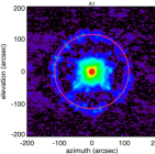
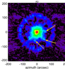
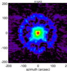
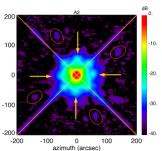
Figure 5: From left to right, beam maps of A1, A3, the combination of the $1\,\rm{mm}$ arrays (A1$\&$3) and the $2\,\rm{mm}$ array (A2) are shown in decibel. These maps, which consist of the normalized combination of four beammap scans of bright point-like sources, are in horizontal coordinates. They represent a zoom in the inner part of larger maps that cover a sky area which extends over $10^{\prime}$. The solid lines and arrows highlight some noticeable features. Red circle in the A1 map (first panel): diffraction ring seen in 1-mm maps (the spokes are presumably caused by radial and azimuthal panel buckling (Greve et al., 2010); Orthogonal yellow lines in the A2 map (rightmost panel): diffraction pattern caused by the quadrupod secondary support structure (prominently seen in A2 map); Yellow arrows in the A3 map (third panel): pattern of 3 spikes seen in $1\,\rm{mm}$ maps of unknown origin; Yellow arrows in A2 map (fourth panel): four symmetrical spikes of the first sidelobes; Pink ellipses: four spikes seen in A2 maps.

Practically, for the production of flux density maps, we perform further selection of the valid KIDs using a conservative noise level threshold of the KIDs at the low level processing, as discussed in Sect. 4. The number of used KIDs for producing science-purpose maps using the data reduction pipeline, as described in Sect. 4, is thus significantly lower than the number of valid KIDs. We evaluate the median number of used KIDs using all scans for each of the observation campaigns. The median fractions of used KIDs with respect to the design ones for each campaigns and for the combinations of all scans are given in Table. 4. We find median fractions of used KIDs of about $70\%$ for the $1\,\rm{mm}$ arrays and of about $80\%$ for the $2\,\rm{mm}$ array, with a notable exception at the N2R9 technical campaign, for which these fraction are lower due to severe atmospheric temperature-induced unstable observing conditions (see Sect. 8.3). Moreover the median fractions of used KIDs are close to the fractions of very stable KIDs from the FOV geometries. We stress that these numbers depend on the choices made in the data reduction pipeline for data sample cuts, and are thus subject to improvement. By contrast, the fractions of valid KIDs $\eta$ constitute a conservative estimates of the stable KIDs usable for science exploitation over all the functioning KIDs. These are thus the relevant estimates for the instrument performance assessment.

6 Beam Pattern

The NIKA2 full beam pattern originates from the KIDs illuminating the internal and external optics, out to the IRAM 30-$\rm{m}$ telescope primary mirror. To characterize the full beam pattern, we use beammap observations. First, deep integration maps of bright sources are produced to provide a qualitative description of the complex beam structure in Sect. 6.1. Then we model the beam using three complementary methods to estimate the main beam angular resolution (Sect. 6.2) and the beam efficiency (Sect. 6.3).

6.1 Full beam pattern

To study the two-dimensional pattern of the beam, we primarily use a map obtained from a combination of beammap observations of strong point sources acquired during the N2R9 commissioning campaign. Namely, we use beammap scans of Uranus, Neptune and the bright quasar 3C84. Furthermore, we checked the stability of our results on single scan maps, combinations of scans for a single source, and combinations of shallower scans but spanning a large range of scanning direction. The beammap scans are reduced using the method discussed in Sect. 4 to produce maps. Figure 5 shows the two-dimensional beam pattern as measured with NIKA2 using the former beammap combination, for each of the arrays and for the $1\,\rm{mm}$ array combination. The beam pattern is shown over a large dynamic range down to about $-40\,\rm{dB}$ and out to radii of about 5’. The telescope beam pattern further extends well beyond this radius, as for example shown by lunar edge observations at the IRAM 30-$\rm{m}$ telescope (Greve et al., 1998; Kramer et al., 2013). However, this extended pattern is at present difficult to detect using the data reduction pipeline discussed in Sect. 4, as the extended error beams are both filtered and mixed with atmospheric and electronics large-scale correlated noise residuals. We expect the filtering effect due to the data processing to become non negligible for angular scales larger than 90”, which corresponds to the radial size of the mask used in the correlated noise subtraction process (see Sect. 4.4). The contributions to the beam pattern that stem from larger angular scales are further discussed in Sect. 6.3.

The NIKA2 beam maps reveal some noticeable features, which are shown in Fig. 5. Ranging from strong and/or extended to weak and/or spiky, they include:

1. the main beam and the underlying first error beam, which is due to large-scale deformations of the primary mirror, and the first side lobes, which correspond to various diffraction patterns. In particular, the 60” and 85” diameter (square-like shaped) side lobes at $1$ and $2\,\rm{mm}$, respectively, at a level lower than $-20\,\rm{dB}$, are due to the convolution of the primary mirror and the quadrupod diffraction pattern with the pixel (KID) transfer function;

2. at a much lower level of about $-30\,\rm{dB}$, a diffraction ring shows up, which is presumably caused by panel buckling of the primary mirror (Greve et al., 2010), as shown with a red circle in the A1 panel;

3. also at a level of about $-30\,\rm{dB}$, the side lobes shown with green diagonal lines in the A2 panel are due to diffraction on the quadrupod holding the secondary mirror of the telescope, as expected from ZEMAX simulations;

4. spikes of not fully understood origin marked by yellow arrows. The ones that are along the vertical and horizontal axes are reproduced by ZEMAX simulations but at a shallower level, whereas the ones shown in the A3 panel in the diagonal directions may be due to the small cylindrical instrumentation box on the side of the M2 cabin. The origin of the asymmetry on the 1 mm arrays is unknown but most probably due to internal optics aberrations;

5. shallow spikes of unknown origin at a level less than $-30\,\rm{dB}$, which are circled by pink ellipses. The multiple images on the combined deep beam map indicate a rotation of these spikes with the observing elevation, which in turn point to diffraction related issue or a ghost image that are formed inside the cryostat. These shallow features are expected to have no significant impact on NIKA2 science results.

We further quantify the respective level of the axi-symmetrical features of the beam pattern by evaluating the beam radial profile $B_{\nu}(r)$, which is the normalized radial brightness profile for the array $\nu$, where $r$ is the radius from the beam center. Although the profile cannot represent the sub-dominant non-axisymmetrical features, which are seen in Fig. 5 (quadrupod diffraction pattern, spikes), it provides a useful representation of the internal and central parts of the beam up to about $180^{\prime\prime}$. We determine a beam profile from a beam map in centring to the fitted value of the main beam center and in computing the weighted average of the map pixels in annular rings.

We checked the stability of the beam against various observing conditions (source intensity, weather condition, focus optimisation) by comparing the beam profiles of a series of 18 beammap observations. This set of beammaps, which is referred to as BM18, has been selected from all the available beammap scans at optimal focus using the baseline scan selection criteria (Sect. 4.6). The measured beam profiles using the BM18 data set are shown in Fig. 6. The profiles consist of the main beam and the first error beams and side lobes, which significantly contribute at levels of less than $-10\,\rm{dB}$ at both observing wavelengths. Moreover, at $1\,\rm{mm}$ the contribution of the diffraction ring, which was marked with a red circle in Fig. 5, is seen as a peak at a level up to $-33\,\rm{dB}$ located at a radius of about $115^{\prime\prime}$. Calculating the rms of the relative difference of the beam profiles to the median beam profile, we find a dispersion below $5\%$ at $1\,\rm{mm}$ and below $2\%$ at $2\,\rm{mm}$.

To measure the relative level of the axi-symmetrical beam pattern features, we further model the beam profiles using an empirical function, which accounts for the main beam and for a significant fraction of the error beams and the side lobes. We define this function $B_{3G}(r)$ as:

$$B_{3G}(r)=\sum_{i=1}^{3}\mathcal{A}_{i}G_{i}(r)+\mathcal{B}_{0},$$ (3)

where $\mathcal{A}_{i}$ is the amplitude of the Gaussian $G_{i}$ for $i\in{1,2,3}$ and $\mathcal{B}_{0}$ a pedestal level accounting for the residual background level in the map. The measured beam profiles are fitted using Eq. 3 and the median best-fit parameters are given in Table 5. The errors are evaluated as the standard deviation of the best-fitting parameter values of the 18 beammap scans of BM18. These values are given to gain insight of beam profile, but are not used for the calibration procedure. We find the level of the first error beam with respect to the total beam at about $-11\,\rm{dB}$ and $-13\,\rm{dB}$ at 1 and $2\,\rm{mm}$, respectively.

Table 5: Median best-fitting values of the parameters of the 3-Gaussian beam profile, as defined in Eq. 3, using the BM18 data set. For $i\in{1,2,3}$ $\bar{\mathcal{A}_{i}}=\mathcal{A}_{i}/\sum{\mathcal{A}_{i}}$. The FWHM for each of the Gaussian are given in arcseconds.

parameters	$1\,\rm{mm}$	$2\,\rm{mm}$
$\bar{\mathcal{A}_{1}}$ [dB]	$-0.33\pm 0.09$	$-0.24\pm 0.03$
$\bar{\mathcal{A}_{2}}$ [dB]	$-11.4\pm 1.0$	$-12.8\pm 0.5$
$\bar{\mathcal{A}_{3}}$ [dB]	$-26\pm 7$	$-27\pm 3$
FWHM1 [”]	$10.8\pm 0.2$	$17.4\pm 0.6$
FWHM2 [”]	$30\pm 2$	$42\pm 3$
FWHM3 [”]	$81\pm 10$	$99\pm 7$

For illustration, we show in Fig. 6 the median three-Gaussian profiles at $1$ and $2\,\rm{mm}$ (pink lines), and the main beam profiles (black lines).

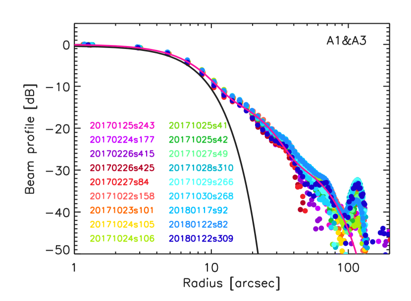
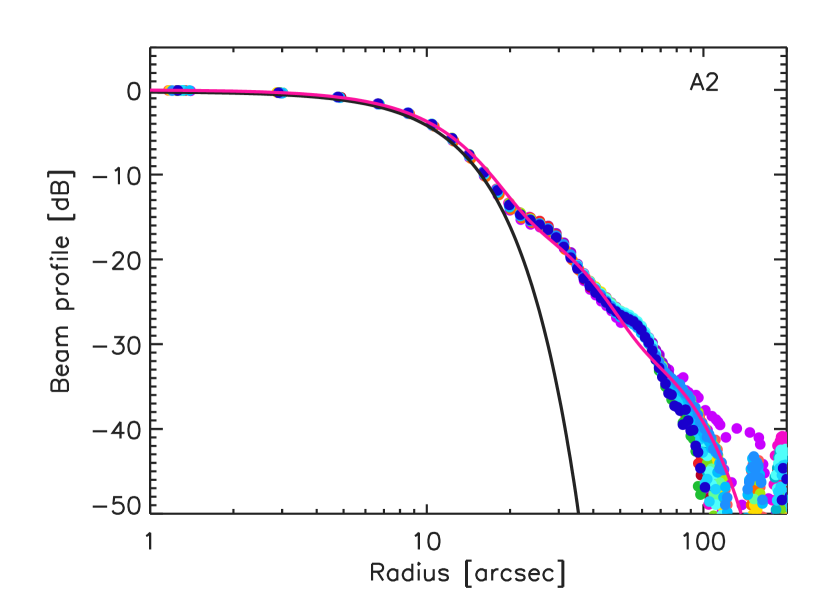
Figure 6: Beam radial profiles given in decibel. The data points are the beam profiles for a series of 18 beammap scans acquired during the reference observational campaigns, labelled from the scan ID. The black line shows the main beam profile using the ’combined’ FWHM, as given in Table 6, while the pink line shows the median best-fit three-Gaussian profile, as defined in Eq. 3.

6.2 Main beam

NIKA2 angular resolution is characterized using the FWHM of a Gaussian fitted to the main beam. This principal Gaussian encloses most of the measured flux density of a point-like source.

6.2.1 Main beam characterization methods

To characterize the main beam and to derive an estimate of its FWHM, we have developed three methods. The two first methods, quoted Prof-3G and Prof-1G, rely on a fit of the beam profile to benefit from the signal-to-noise ratio increase after azimuthally averaging the signal. The last one by contrast, consists in an elliptical Gaussian fit of the beam map for a better 2D modelling, and is labelled Map-1G. They are presented in more detail below.

Prof-3G consists in fitting the beam profile using the three-Gaussian function defined in Eq. 3. The main beam FWHM estimate is given by the best-fitting value of the FWHM for the first Gaussian function. This main beam FWHM estimate is expected to be immune to the first error beams and side lobes, which are well accounted for. For consistency checks, we also relies on two other methods that rely on simpler beam models.

Prof-1G relies on fitting a single Gaussian to the beam profile after masking the portion of the profile where the contributions of the side lobes and error beams are the largest. Specifically, the side lobe mask is designed to cut out the radius ranging from an inner radius $r_{\rm{in}}=0.65\,\mathrm{FWHM}_{0},$, where FWHM₀ is the reference Gaussian beam FWHM (see Sect. 8.1.1) to an outer radius $r_{\rm{out}}=80^{\prime\prime}$, centred on the beam maximum. The profile is estimated up to a radius of $180^{\prime\prime}$, that is in the inner part of the beam map where the noise variance is uniform.

Map-1G consists in modelling the two-dimensional distribution of the main beam using an 2D elliptical Gaussian of size $\sigma_{x}$ and $\sigma_{y}$. We characterize the NIKA2 main beam using

$$FWHM=2\sqrt{2\ln{2}\,\sigma_{x}\sigma_{y}}.$$ (4)

As in Prof-1G, we use masked versions of the beam map to avoid side lobe and error beam contaminations. Whereas $r_{\rm{out}}$ is conservatively set to be $100^{\prime\prime}$, $r_{\rm{in}}$ is let free to vary around a central value of about $8^{\prime\prime}$ for A1 and A3 and of about $12^{\prime\prime}$ for A2 to provide the best 2D Gaussian fit.

6.2.2 Data sets for the main beam determination

We select a sub-set of the selected beammap scans described in Sect. 6.1 by discarding scans of Mars. Indeed, beammaps towards Mars unveil the complex full beam pattern, which extends beyond radii of $100^{\prime\prime}$, so that the annulus sidelobe mask used in Prof-1G and Map-1G is not sufficient to mitigate the error beams and sidelobes effects. The 12 remaining beammap scans are analysed using the data reduction pipeline of Sect. 4 and projected onto maps with a resolution of $1^{\prime\prime}$ and an angular size of $10^{\prime}$. This data set is referred to as BM12.

We also consider series of shorter integration scans. We select $5^{\prime}\times 8^{\prime}$ raster scans of moderately bright to very bright point sources by thresholding the flux density estimates at $1\leavevmode\nobreak\ \rm{Jy}$ at both wavelengths. After the baseline scan selection, as described in Sect. 4.6, the data set comprises 154 scans towards the giant planets Uranus and Neptune, the secondary calibrator MWC349 and the quasars 3C84, 3C273, 3C345 and 3C454 (aka 2251+158). For these short scans, which are referred to as R154, the data are reduced and projected onto $2^{\prime\prime}$ resolution maps.

Finally, we use a series of 75 observation scans of Uranus and Neptune, which includes both beammap and $5^{\prime}\times 8^{\prime}$ raster scans. This data set, which is referred to as UN75, consists of all the scans of Uranus and Neptune acquired during the reference observation campaigns (N2R9, N2R12 and N2R14).

6.2.3 Results

We have derived the main beam FWHM for the three arrays and the $1\,\rm{mm}$ arrays combination using the three methods presented in Sect. 6.2.1 and the data sets of Sect. 6.2.2. Namely, our main beam FWHM estimates consist of i) the median FWHM estimate using Prof-3G on the BM12 dataset, ii) the average FWHM estimate using Prof-1G on the UN75 data set and the Map-1G average FWHM using either BM12 or R154. By comparing these results, we test the stability of the FWHM estimates against the choices of the data set and of the estimation method.

In the case of Uranus, the FWHM estimates are further corrected for the average beam broadening induced by the extension of the apparent disc of the planet, which is $0.19^{\prime\prime}$ and $0.12^{\prime\prime}$ at 1 and $2\,\rm{mm}$, respectively. During the observation period, Uranus disc diameter has varied from $3.3^{\prime\prime}$ to $3.7^{\prime\prime}$. This diameter variation translates into beam broadening variations of an amplitude of a few tenth of arcseconds, which are neglected.

The results of this analysis are gathered in Table 6, including uncertainties evaluated as the rms dispersion of single-scan based FWHM estimates. Prof-1G and Map-1G results are in agreement within uncertainties, whereas Prof-3G yields slightly smaller FWHM. The latter is more robust against the error beams and large radii beam features than the formers, as expected. Combined results are obtained from an error-weighted average of the four FWHM estimates for each array. Because the rms errors estimated using the 12 beammap scans may be optimistic considering the small statistic, they are conservatively increased to match the uncertainty estimates based on the R154 data set before performing the weighted average. The combined results, as given in Table 6, provide a robust evaluation of the FWHM. Hence, we report main beam FWHMs of $11.1^{\prime\prime}\pm 0.2^{\prime\prime}$ at $1\,\rm{mm}$ and $17.6^{\prime\prime}\pm 0.1^{\prime\prime}$ at $2\,\rm{mm}$.

Table 6: Estimates of the main beam FWHM in arcsec, using three estimation methods (see Sect. 6.2.1) and three data sets (see Sect. 6.2.2), and their combination.

Method	Dataset	FWHM [”]
		A1	A3	A1 $\&$ A3	A2
Prof-3G	BM12	$10.8\pm 0.1$	$10.8\pm 0.1$	$10.8\pm 0.1$	$17.4\pm 0.1$
Prof-1G	UN75	$11.3\pm 0.4$	$11.2\pm 0.4$	$11.2\pm 0.3$	$17.4\pm 0.2$
Map-1G	R154	$11.3\pm 0.2$	$11.1\pm 0.2$	$11.2\pm 0.2$	$17.8\pm 0.1$
	BM12	$11.2\pm 0.1$	$11.1\pm 0.1$	$11.2\pm 0.1$	$17.6\pm 0.1$
Combined		$11.1\pm 0.2$	$11.0\pm 0.2$	$11.1\pm 0.2$	$17.6\pm 0.1$

6.2.4 Stability checks

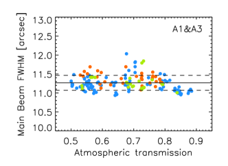
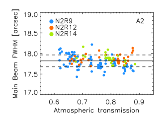
Figure 7: Main beam FWHM estimates for the $1\,\rm{mm}$ (top) and $2\,\rm{mm}$ (bottom) channels are shown as a function of the atmospheric transmission estimated at the corresponding wavelengths using bright point source observations acquired during the reference observation campaigns (N2R9, N2R12, N2R14).

Figure 7 shows the main beam FWHM estimates using Map-1G as a function of atmospheric transmission, which is modelled as $\exp{\left(-\tau_{\nu}\,x\right)}$. The main beam FWHM estimates using data of the three campaigns are in agreement within rms errors. Moreover, the main beam FWHM is stable against atmospheric conditions at both wavelengths. Slightly lower values than average (about $11^{\prime\prime}$) are observed in the best atmospheric conditions at $1\,\rm{mm}$ providing us with a lower limit in the absence of correlated atmospheric noise residuals. We note three scans acquired during the N2R12 campaign with larger FWHM than average at $2\,\rm{mm}$ although the atmospheric transmission was excellent: this is likely an effect of atmospheric instabilities, which affected a large number of observation scans during N2R12.

6.3 Main beam efficiency

We derive the main beam efficiency for each array, which is defined as the ratio of the solid angle sustained by the main beam to the total beam solid angle.

To estimate the total beam solid angle, we primarily use the maps of the beam pattern presented in Sect. 6.1, which provide us with accurate representation of the main beam and of the first error beams. However, at angular scales larger than the radius of the noise decorrelation mask, 90”, the filtering effect induced by the data processing becomes non negligible (see also Sect. 4). Furthermore, heterodyne observations at the IRAM 30-$\rm{m}$ telescope towards the lunar edge and estimates of the forward beam efficiency using skydips show that a significant fraction of the full beam stems from angular scales much larger than $90^{\prime\prime}$ (Greve et al., 1998; Kramer et al., 2013). Thus, the accurate assessment of the total beam solid angle requires to account for the filtering effect and the large angular scales contributions. To that aim, we resort to an hybrid approach. We utilize both the full beam pattern measurements with NIKA2 as presented in Sect. 6.1, and the results of the IRAM 30-$\rm{m}$ telescope beam pattern characterization using EMIR front-end observations (Carter et al., 2012), as reported in Kramer et al. (2013). These results came in two flavours.

First, the main beam and error beams are measured using observations towards the limbs of the Moon. As EMIR detectors were coupled to the 30-$\rm{m}$ telescope entrance pupil via corrugated horns, the contribution of the first error beam is significantly attenuated compared to the NIKA2 case. In fact, the first error beam measured by NIKA2 is not detected with EMIR, while the second error beam is measured with both NIKA2 and EMIR at compatible levels. The third and fourth error beams, which originate from the IRAM 30-$\rm{m}$ telescope frame misalignment and panel deformations, respectively, are expected to be measured by EMIR without attenuation (Kramer et al., 2013). We assume these latter are characteristics of the 30-$\rm{m}$ telescope without any significant dependencies on the receiver instrument.

Second, the IRAM 30-$\rm{m}$ telescope forward efficiencies $F_{\rm{eff}}$ are derived using skydip scans with EMIR. Their measurements allow us to estimate the far side lobes efficiencies, which receive two different contributions. The forward spillover and scattering efficiencies are estimated as $F_{\rm{eff}}$ subtracted from the main beam and error beams efficiencies, and the rearward spillover and scattering efficiencies equal $1-F_{\rm{eff}}$ (Kramer et al., 2013).

To sum up, we estimate the solid angle of the total beam as

$$\begin{split}\Omega_{\rm{tot}}(\nu)=&\int_{0}^{2\pi}\left(\tilde{B}_{\nu}(r)+\mathcal{A}_{\nu}^{(3)}G_{\nu}^{(3)}(r)+\mathcal{A}_{\nu}^{(4)}G_{\nu}^{(4)}(r)\right)2\pi rdr\\ &+\,\Omega_{\rm{FSL}}(\nu),\end{split}$$ (5)

where $\tilde{B}_{\nu}(r)$ is the normalised beam profile $B_{\nu}(r)$ for the array $\nu$, as discussed in Sect. 6.1, after rescaling with a factor of $(1-\mathcal{A}_{\nu}^{(3)}-\mathcal{A}_{\nu}^{(4)})$; $\mathcal{A}_{\nu}^{(3)}$ and $\mathcal{A}_{\nu}^{(4)}$ are the amplitudes of the third and fourth Gaussian error beams $G_{\nu}^{(3)}$ and $G_{\nu}^{(4)}$, respectively, which are measured with EMIR and extrapolated for the array $\nu$ following the prescription given in Kramer et al. (2013); $\Omega_{\rm{FSL}}(\nu)$ is the contribution of the far side lobes to the total beam solid angle of the array $\nu$, as derived from $F_{\rm{eff}}$ measurements.

In addition, for cross-checks and stability tests, we also compute the total beam solid angle up to a maximum radius

$$\Omega_{r_{\rm{max}}}(\nu)=\int_{0}^{r_{\rm max}}B_{\nu}(r)\,2\pi rdr,$$ (6)

where $r_{\rm{max}}$ is taken as the largest radius for which the filtering effect of the data processing has no significant impact. We take $r_{\rm{max}}$ as the radius of the noise decorrelation mask, which is 90” and evaluate $\Omega_{90}$ from the measured beam profiles obtained using the UN75 data set (see Sect. 6.2.2). Results per observational campaigns, with uncertainties evaluated as the rms scatter on the average, are given in Table 7. The $\Omega_{90}$ estimates are statistically compatible from one campaign to another with some variations of the average value due to the dispersion in the focus settings and atmospheric conditions that prevail during each campaign. The combined results, based on the whole UN75 data set, are the inverse-variance weighted average of the $\Omega_{90}$ for the three campaigns, while the error bars are conservatively estimated as the maximum half-difference between the $\Omega_{90}$ estimates.

Table 7: Estimates of the solid angle of the beam up to a radius of $90^{\prime\prime}$, $\Omega_{90}$, and rms uncertainties given in arcsec² using Neptune and Uranus scans acquired during three observation campaigns, and the combined result. For each case, the number of scans is given in the column labelled ’nbs’.

Campaign	nbs	A1	A3	A1&A3	A2
N2R9	27	245$\pm$20	233$\pm$18	239$\pm$15	452$\pm$16
N2R12	20	209$\pm$9	203$\pm$8	206$\pm$7	422$\pm$9
N2R14	28	232$\pm$14	228$\pm$18	230$\pm$14	441$\pm$14
Combined	75	219$\pm$18	211$\pm$15	215$\pm$17	432$\pm$15

The main beam solid angle is evaluated from the main beam (mb) FWHM, as $\Omega_{\rm{mb}}=2\pi\,\sigma_{\rm{mb}}^{2}$, where FWHM$=2\sqrt{2\ln{2}}\,\sigma_{\rm{mb}}$. The main beam efficiency

$$\rm{BE}=\frac{\Omega_{\rm{mb}}}{\Omega_{\rm{tot}}}$$ (7)

is evaluated using both the UN75 and the BM12 data sets, as presented in Sect. 6.2.2. For cross-checks, we compare the results based on three estimates of the total beam and main beam solid angles:

• BE1 relies on the best-fitting parameters of the three-Gaussian model of the full beam, as given in Eq. 3, to derive both the main beam solid angle and the two first errors beam contributions to the total beam solid angle. The main beam solid angle thus corresponds to the volume enclosed by the first Gaussian, as obtained using Prof-3G, while the normalised beam profile in Eq. 5 is the normalised best-fitting $B_{3G}(r)$;

• BE2 consists in using the normalised beam profile measurements from the UN75 data set to estimate $\Omega_{\rm{tot}}$, while $\Omega_{\rm{mb}}$ is derived with the FWHM obtained using Prof-1G (see Sect. 6.2.1);

• BE3 is similar to BE2 but relies on the BM12 data set, while the main beam FWHM is derived using Map-1G.

For all methods, the contributions of the third and fourth error beams and of the far side lobes, which enters in Eq. 5, are the same.

The main beam efficiency estimates using the three methods are gathered in Table 8: central values and error bars are evaluated as the median and the rms error of the estimates on individual observation scans, respectively. We combined the results of the three methods, which are in agreement with each others, using an inverse variance-weighted average and a quadratic mean of the rms uncertainties. The main beam efficiency uncertainties, as given in Table 8, also include uncertainties on the third and fourth error beam contributions and on the 30-$\rm{m}$ telescope forward efficiencies, as reported in Greve et al. (1998); Kramer et al. (2013). Using the combined results, we report main beam efficiencies of $47\pm 3\%$ at $1\,\rm{mm}$ and $64\pm 3\%$ at $2\,\rm{mm}$.

Table 8: Main beam efficiency estimated for each array or array combination, using three different methods, and the combined results, given in percent.

Method	A1	A3	A1 $\&$ A3	A2
BE1	$46\pm 2$	$47\pm 2$	$47\pm 3$	$62\pm 3$
BE2	$45\pm 4$	$46\pm 4$	$45\pm 4$	$63\pm 3$
BE3	$49\pm 3$	$50\pm 3$	$50\pm 3$	$64\pm 2$
combined	$47\pm 3$	$48\pm 3$	$47\pm 3$	$64\pm 3$

Table 9: Estimates of the total beam solid angle and main beam efficiency including in turn further contributions to the full beam ranked by their angular scales (see text). All solid angles are given in arcsec², while the main beam efficiencies are in percent.

	A1&A3	A2
$\Omega_{90}$	211 $\pm$ 12	434 $\pm$ 13
$\Omega_{\rm{hyb}}$	264 $\pm$ 13	504 $\pm$ 13
$\Omega_{\rm{tot}}$	290 $\pm$ 14	541 $\pm$ 18
$\rm{BE}_{90}$	64 $\pm$ 5	80 $\pm$ 3
$\rm{BE}_{\rm{hyb}}$	52 $\pm$ 3	69 $\pm$ 2
$\rm{BE}$	47 $\pm$ 3	64 $\pm$ 3

Finally, we compute the total beam solid angle and main beam efficiency using the combination of the three previously described methods, in three cases that successively include larger angular scale contributions to the full beam: $\Omega_{90}$ and $\rm{BE}_{90}$ are the total beam solid angle and main beam efficiency integrated up to $90^{\prime\prime}$, which include the main beam and the two lower angular scales error beams, as measured in NIKA2 beam maps; $\Omega_{\rm{hyb}}$ and $\rm{BE}_{\rm{hyb}}$ further account for the third and fourth error beams, as derived from EMIR front-end measurements; $\Omega_{\rm{tot}}$ and $\rm{BE}$ are the final estimates that comprise all beam contributions. The results are given in Table 9 for the 1 mm and 2 mm channels. These give insight on the relative importance of the contributions at various angular scales. For example, 18$\%$ and 13$\%$ of the total beam solid angle stem mainly from the two largest error beams integrated at angular scales larger than 90”, and 9$\%$ and 7$\%$ originate from the far side lobes at 1 and 2 mm respectively.

7 Atmospheric opacity

The atmospheric opacity constitutes the ultimate limitation of ground-based experiments. Only a fraction of the source signal is transmitted by the atmosphere and reaches NIKA2 detectors. The relation between the observed flux density $\tilde{S}_{\nu}$ and the top-of-the-atmosphere flux density $S_{\nu}$ is parametrized by the zenith opacity $\tau_{\nu}$ and the air mass $x$ as

$$\tilde{S}_{\nu}=S_{\nu}\,e^{-\tau_{\nu}x}.$$ (8)

An accurate derivation of the atmospheric opacity for each scan is of the utmost importance to retrieve the source signal and thus, to ensure small calibration uncertainties. We developed three atmospheric opacity derivation methods, which are described in Sect. 7.1. In Sect. 7.2, we present robustness tests.

7.1 Atmospheric opacity estimation

We have developed three procedures for the atmospheric opacity derivation: i) taumeter relies on measurements provided by the resident IRAM taumeter operated at $225\,\rm{GHz}$; ii) skydip consists in using NIKA2 as a total-power taumeter by resorting to a series of skydip scans; iii) corrected skydip is a modified version of the skydip method that minimizes the dependence of the estimated flux density on the opacity.

All methods i) do not rely on an ATM model nor on any hypothesis on the atmospheric contents for the sake of robustness, and ii) do not use the laboratory measurements of the bandpass (see Sect. 2.5) for more accuracy.

Sect 7.1.1 presents the taumeter method. The skydip method is described in Sect 7.1.2 and the selection of the used skydip scans is discussed in Sect. 7.1.3. corrected skydip is presented in Sect. 7.1.4.

7.1.1 The taumeter method

The IRAM 30-$\rm{m}$ telescope facility is equipped with a resident taumeter operated at 225 GHz. Every four minutes, it performs elevation scans at fixed azimuth to monitor the atmospheric opacity. The IRAM science support team provides us with time-stamped zenith opacities at $225\,\rm{GHz}$ $\tau_{225}$, as derived from the taumeter measurements. The $\tau_{225}$ estimates come in two different flavours: one relying on a linear model and the other on an exponential fitting model. They are then filtered by removing outliers and by using a threshold on goodness-of-fit criteria. Based on IRAM experience, we use the linear fit and filtered $\tau_{225}$ data for the NIKA2 analysis. The time-stamped $\tau_{225}$ estimates, which are sampled about every 4 minutes, are interpolated to the time of the NIKA2 scans (we consider the time of the middle of the scan). For cross-check we also produce a smooth version of time-stamped $\tau_{225}$ data by filtering with a running median of seven samples, which is then interpolated to the NIKA2 scan times.

We fit the relations between the IRAM $225\,\rm{GHz}$ taumeter opacities and NIKA2 band pass opacities using observation of calibration sources which spans a large range of air masses. This method has the advantages of not relying on atmospheric model nor on the bandpass measurements in laboratory. We use a series of 64 scans of MWC349, which consists of the baseline selected subset of scans from the 68 available scans for this source during N2R9. It constitutes an homogeneous data set in flux density but heterogeneous in atmospheric conditions: zenith opacities at $225\,\rm{GHz}$ range from 0.08 to 0.32 and elevations from $23$ to $73$ degrees, spanning a large range of air mass as required. NIKA2 opacities $\tau_{\nu}$, for $\nu$ corresponding to the observing frequency of Array 1, 2, 3 and the combination of Arrays 1 and 3, are estimated from the $225\,\rm{GHz}$ taumeter median-filtered linear-based opacity estimates $\tau_{225}$ as

$$\tau_{\nu}=a_{\nu}^{225}\tau_{225}+b_{\nu}^{225}.$$ (9)

The parameters $a_{\nu}^{225}$ and $b_{\nu}^{225}$ are fitted to the data set so that the source flux density

$$S_{\nu}=\tilde{S}_{\nu}\,\,e^{(a_{\nu}^{225}\tau_{225}+b_{\nu}^{225})\,x},$$ (10)

is constant within scans.

Table 10: Best-fit parameters and rms uncertainties to infer NIKA2 opacities from the IRAM taumeter measurements.

Parameters	Array 1	Array 3	Array 1$\&$3	Array 2
$a_{\nu}^{225}$	$1.94$	$1.90$	$1.92$	$0.94$
$b_{\nu}^{225}$	$-0.04$	$-0.07$	$-0.06$	$0.00$
$\Delta a_{\nu}^{225}$	$0.15$	$0.08$	$0.09$	$0.10$
$\Delta b_{\nu}^{225}$	$0.05$	$0.03$	$0.04$	$0.03$

We tested two estimators of the flux stability. The first one relies on minimizing the standard deviation of the measured-to-median flux densities ratio after atmospheric opacity correction using Eq. 10. The second one is obtained by minimizing

$$\chi^{2}=\sum_{i=1}^{N}\frac{1}{\sigma^{2}}\,\left(\frac{S_{\nu}}{\rm{Med}(S_{\nu})}-1\right)^{2},$$ (11)

where $\sigma$ is the rms uncertainty of the flux density estimates. Note that these estimators do not depend on the absolute scale of the flux density of the source. Both estimators yield consistent results that are combined and gathered in Table. 10. The quoted errors $\Delta a_{\nu}^{225}$ and $\Delta b_{\nu}^{225}$ are 1-$\sigma$ errors of the fit.

We note that the atmospheric opacity correction using taumeter opacities yields stable flux density measurements with respect to the atmospheric transmission by construction, as we will verify in Sect. 9. This means that the best-fitting parameters of the model in Eq. 9 also correct for any line-of-sight opacity dependent systematic effects on the flux densities, as it will be further discussed in Sect. 7.1.4 and Sect. 7.2.

Because the IRAM taumeter observes at a fixed azimuth, the taumeter opacities are not the line-of-sight opacities for the observation scans. As this will be checked in Sect. 9, this induces larger rms errors of the top-of-the-atmosphere flux density estimates compared to opacity correction methods that relies on NIKA2 skydip-based measurements. The taumeter method will thus be used as an alternative method in case of failure of the NIKA2 skydip-based methods and to perform consistency checks.

7.1.2 NIKA2 skydip-based method

The NIKA2 skydip method for the opacity derivation consists in using the NIKA2 instrument as an in-band total-power taumeter. The opacity integrated in the NIKA2 bandpasses and in the line-of-sight of the observing scan is thereby directly obtained. This idea, which was successfully tested with NIKA (Catalano et al., 2014), relies on the fact that the resonance frequency of each KID varies linearly with the total power, as discussed in Sect. 2.4. First, we have to calibrate the relationship between total power and opacity. Then, we can use this calibration to measure the opacity during a given scan.

First, we detail the opacity calibration. For each KID $k$, the absolute value of its resonance frequency $f_{\rm{reso}}^{k}$ varies with the atmospheric load according to

$$f_{\rm{reso}}^{k}=c_{0}^{k}-c_{1}^{k}T_{\rm{atm}}[1-e^{-\tau_{\nu}x}]$$ (12)

where $c_{0}^{k}$ is a constant equal to the KID resonance frequency at zero opacity, $c_{1}^{k}$ is a calibration conversion factor in Hz$/$K, $T_{\rm{atm}}$ is the temperature of the atmosphere. By assuming a homogeneous plane-parallel atmosphere, the air mass $x$ is defined from the elevation as $x=\left(\sin\rm{el}\right)^{-1}$. The Earth sphericity can be safely neglected at the elevations under discussion here. We take $T_{\rm{atm}}$ as a constant equal to 270 K. However, the opacity is expected to slightly depend on the atmospheric temperature. For example, in poor weather conditions (6 mm of water vapour contents), the zenith opacity in both observing bands can vary by about 10% for temperature variations of 10 K. The effect of the temperature variations on the final calibration of NIKA2 response to the sky load is mitigated by using several dedicated observation scans regularly distributed all along an observation campaign.

The $c_{0}^{k}$ and $c_{1}^{k}$ are determined using skydip scans, which consist in moving the telescope in elevation step by step, as defined in Sect. 3.3. For each KID $k$, the evolution of $f_{\rm{reso}}^{k}$ is monitored as a function of the air mass in each elevation step to perform a joint fit of the zenith opacity $\tau_{\nu}$ and the $c_{0}^{k}$ and $c_{1}^{k}$ coefficients. All skydips, obtained under various opacity conditions, are analysed together to break the degeneracy between the opacity and the Hertz-to-Kelvin conversion factor $c_{1}^{k}$. The degeneracy occurs mostly for low opacity conditions for which we can only determine the combination $c_{1}^{k}\tau_{\nu}x$. The procedure has two steps. First, all the skydip scans are analysed individually to extract $f_{\rm{reso}}^{k}$ for each stable elevation and for each KID. Secondly, a simultaneous fit is done for all parameters (one $\tau_{\nu}$ per skydip, and a set of $c_{0}^{k}$ and $c_{1}^{k}$ for all KIDs). Figure 8 illustrates the fitting procedure.

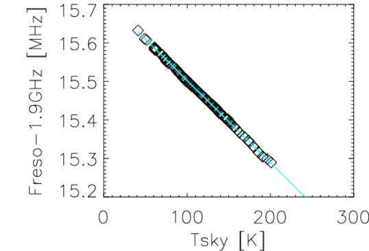
Figure 8: Example of the global skydip fit for a KID. Each square point represents one step in a skydip (made of eleven elevation steps). A series of 12 skydip scans are jointly used spanning zenith opacities from 0.15 to 0.50 in the $1\,\rm{mm}$ band. The horizontal axis gives the sky effective temperature $T_{\rm{sky}}=T_{\rm{atm}}[1-e^{-\tau_{\nu}\,x}]$ in Kelvin, where $\tau_{\nu}$ is the skydip zenith opacity found in the fit. The vertical axis shows the relative resonance frequency of the KID with respect to 1.9 GHz, given in MHz. The blue line is the linear model using the best-fit $c_{0}^{k}$ and $c_{1}^{k}$ coefficients (see Eq. 12).

This fit is performed on block of 40 KIDs. We check that the resulting $\tau_{\nu}$ from the different blocks are consistent within rms errors, which are equal to about $4\times 10^{-3}$ at 1 mm and $1\times 10^{-3}$ at 2 mm. Once the $\tau_{\nu}$ values are estimated for each skydip (as the average over the blocks), we compute, while fixing the $\tau_{\nu}$, the $c_{0}^{k}$ and $c_{1}^{k}$ final values for each KID $k$ with a linear fit. We thus retrieve the coefficients of all the KIDs even though some of them could not contribute to the $\tau_{\nu}$ determination.

We have observed that the $c_{0}^{k}$ and $c_{1}^{k}$ coefficients vary between observational campaigns due to a change in the KID properties from one cool-down to another. However, by comparing the results of different skydips, we have verified that the coefficients $c_{0}^{k}$ and $c_{1}^{k}$ are stable, within the fitting errors, on very long time scales within a cool-down cycle. The coefficients can thus be applied to the whole observing campaign for the opacity derivation. Specifically, the opacity is retrieved for each observation scan by inverting Eq. 12 as:

$$\tau_{\nu}=\rm{Med}\left(-\frac{1}{x}\log\left(\frac{f_{\rm{reso}}^{k}-c_{0}^{k}}{c_{1}^{k}T_{\rm{atm}}}+1\right)\right),$$ (13)

where the median is evaluated using all the valid KIDs of the arrays under concern. Hence, we are able to derive an opacity integrated in the NIKA2 bandpasses and in the line-of-sight of the source in the considered observation scan.

7.1.3 Skydip scan selection

The skydip opacity derivation requires to have on hands a sizeable amount of skydip scans – typically ten to twenty – that i) span the whole opacity range and ii) avoid highly perturbed atmosphere to meet the plane-parallel atmosphere assumption. To that aim, we perform a skydip scan twice a day during a scientific campaign. Then, the ($c_{0}^{k}$, $c_{1}^{k}$) determination process relies on a selection of the skydip scans.

For each skydip scan and for each KID, we compute the difference between the measured KID resonance frequency and the model given in Eq. 12 taken at the best-fit values of the ($c_{0}^{k}$, $c_{1}^{k}$) parameters, which is named $df_{\rm{reso}}^{k}$. Then, we determine two indicators of the fit quality per skydip. First, for each block of 40 KIDs, the standard deviation of $df_{\rm{reso}}^{k}$ is calculated over all the KIDs of the block. This standard deviation per KID block is called $\sigma_{40}$. For each skydip, we evaluate the median rms, which is the median $\sigma_{40}$ over all the KID blocks.

Figure 9: Median dT quality-fit criterion is plotted as a function of the median rms criterion for each skydip scan of the N2R9 campaign and for the three arrays. The skydips that yield a poor fit of the KID resonance frequencies and hence do not met Median dT criterion, are also discarded using Median rms. The latter criterion further discards noisy skydips. Empty diamonds show the results of the first iteration of the skydip coefficient estimation, labelled ’v1’, whereas filled circles show the second iteration, labelled ’v2’, for which only the skydips that met both fit-quality criteria are included. After the second iteration, all the remaining skydips met the criteria.

This fit quality indicator is also sensitive to the noise level during the skydip. We therefore devise a second fit quality indicator to further measure the bias between the data and the best-fit model. Namely, for each skydip, we compute the average $df_{\rm{reso}}^{k}$ of each KID $k$ and convert this quantity from Hertz to Kelvin using the corresponding $c_{1}^{k}$ parameter. This cross-calibration allows us to compare the $df_{\rm{reso}}^{k}$ estimates from different KIDs. Median $dT$ is the median of the average $df_{\rm{reso}}^{k}$ in Kelvin over all the KIDs of an array. With these two indicators in hands, we discard the skydip scans that are noisy or that yield a poor fit by applying the following selection criteria:

• Median $\rm{rms}<1.5\times 10^{4}\leavevmode\nobreak\ \rm{Hz}$

• Median $dT<1.6\leavevmode\nobreak\ \rm{K}$

The threshold values have been determined using the set of 44 skydip scans of N2R9. The Median rms cut corresponds to twice the median of this quantity per skydip scan, whereas the Median $dT$ cut is twice the standard deviation of Median $dT$ over the skydip scans. N2R9 skydip scan selection is illustrated in Fig. 9, which shows the complementarity between the two fit-quality criteria. After selection, 15 skydips are kept for the final step of the ($c_{0}^{k}$, $c_{1}^{k}$) fit in the case of the N2R9 campaign.

The ($c_{0}^{k}$, $c_{1}^{k}$) estimation proceeds in two steps: first the parameters are estimated using all the available skydip scans for a given campaign, then the estimation is repeated using only skydip scans that met the fit-quality criteria. After the second iteration, we check that no extra skydip scan outliers are left, as shown by the ’v2’ label data points in Fig. 9.

\begin{overpic}[clip={true},trim=0.0pt -8.5359pt -8.5359pt 0.0pt,width=130.08731pt]{Figures/Opacity_correl_skydip_vs_tau_a1.pdf} \put(0.0,70.0){\footnotesize a)} \end{overpic}

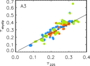
\begin{overpic}[clip={true},trim=-8.5359pt -8.5359pt 0.0pt 0.0pt,width=130.08731pt]{Figures/Opacity_skydip_to_taumeter_vs_elev_1mm.pdf} \put(0.0,70.0){\footnotesize b)} \end{overpic}

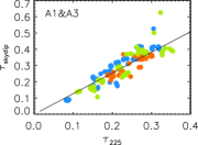
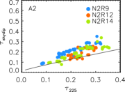
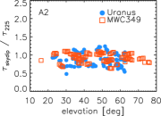
Figure 10: NIKA2 skydip-based opacities $\tau_{\nu}^{\rm{skydip}}$ consistency checks. a) $\tau_{\nu}^{\rm{skydip}}$ vs median-filtered time-stamped IRAM 225 GHz taumeter opacities (see Sect. 7.1.1). For illustration purpose, the modelled correlations relying on an ATM model integrated in NIKA2 frequency bands are shown in black. b) $\tau_{\nu}^{\rm{skydip}}$ stability against the observing elevation. The ratio between the skydip-based opacities and the taumeter-derived opacities is shown as a function of the observing elevation as blue points for Uranus scans and empty red square for MWC349 scans. See discussion in Sect. 7.2.

The stability of the ($c_{0}^{k}$, $c_{1}^{k}$) parameters and hence the skydip opacity estimates, have been tested against the choice of the selection criteria. We found that the $\tau_{\nu}$ estimates are robust against the skydip-scan selection as long as the selection includes good skydip scans in high opacity condition $(\tau_{1\rm{mm}}>0.44)$ and as the poor fitting skydip scans, which mostly correspond to deviation from the atmosphere plane-parallel model in high opacity skydip scans (as seen in Fig. 9), are excluded.

7.1.4 Corrected skydip

The opacity estimates are ultimately tested by assessing the stability of the top-of-the-atmosphere flux densities of bright sources for a large range of atmospheric conditions, as will be addressed in Sect. 9. After opacity correction using the skydip $\tau_{\nu}$ estimate, the calibration flux density measurements show a residual dependency on the atmospheric transmission, as discussed in Sect. 9. This has motivated the development of a corrected version of the skydip method that ensures the robustness of the flux densities against atmospheric conditions.

As already noticed in Sect. 7.1.2, for small values of the line-of-sight opacity $\tau_{\nu}x$, only the parameter combination $c_{1}^{k}T_{\rm{atm}}\tau_{\nu}$ is constrained in Eq. 12. Degeneracies between $c_{1}^{k}$ parameters, the atmospheric temperature and $\tau_{\nu}$ can translate into a scaling factor in the fitted skydip opacities $\tau_{\nu}^{\rm{skydip}}$. To take this effect into account, we use the flux stability estimators described in Sect. 7.1.1 to fit a correction to $\tau_{\nu}^{\rm{skydip}}$ as

$$\tau_{\nu}=a_{\nu}^{\rm{skydip}}\tau_{\nu}^{\rm{skydip}}.$$ (14)

We find $a_{\nu}^{\rm{skydip}}$ of $1.36\pm 0.04$, $1.23\pm 0.02$, $1.27\pm 0.03$ and $1.03\pm 0.03$ for A1, A3, A1$\&$A3 and A2 respectively.

Moreover, we test for an additional offset in the correcting relation of the skydip opacities given in Eq. 14. We find best-fitting correcting factors in agreement with the best-fit values estimated using the single-parameter correcting relation, whereas the best-fit offsets are compatible with zero at both wavelengths. We conclude that correcting the skydip opacity estimates for a normalisation as given in Eq. 14 suffices for ensuring flux density robustness against atmospheric opacity conditions.

The exact physical origin for the discrepancy of the empirical factor $a_{\nu}^{\rm{skydip}}$ from the expected unity value for the $1\,\rm{mm}$ wavebands is currently under investigation. Beside the $c_{1}^{k}$-to-$\tau_{\nu}$ degeneracy and the effect of the variation of the atmospheric temperature, other explanations include effects that are not directly related to the atmospheric opacity derivation, as the empirical factor is measured on the flux densities. However, the stability of the flux densities corrected using the corrected skydip opacities and the results consistency using several observation campaigns, as discussed in Sect. 9, constitutes a validation of this approach.

7.2 Opacity estimate consistency checks

First, we test the stability of the skydip opacities from one observation campaign to another. Panels a) in Fig. 10 show the correlation between the skydip $\tau_{\nu}$ estimates $\tau_{\nu}^{\rm{skydip}}$ and the median-filtered time-stamped IRAM $225\,\rm{GHz}$ taumeter zenith opacities $\tau_{225}$, as described in Sect. 7.1.1, for a series of scans of Uranus and MWC349 acquired during the reference observation campaigns. As guidelines, we also show the predicted correlations using an ATM model integrated in the NIKA2 bandpasses and in the $225\,\rm{GHz}$ band. The $\tau_{\nu}^{\rm{skydip}}$ to $\tau_{225}$ correlation relations are consistent within statistical errors for the three campaigns. At 1 mm they are also in agreement with the ATM model expectations, while at 2 mm the ATM model underestimates the measured skydip $\tau_{\nu}$. Possible explanations include a ground pick-up effect, which would have comparatively more impact on the opacity derivation at 2 mm, where the atmosphere is more transparent, than at 1 mm. Indeed a fraction of the beam detects radiation from the ground, as evidenced by forward efficiency measurements using heterodyne front-ends (see Sect. 6.3). This mild discrepancy with the ATM model predictions is yet to be understood, but has no impact on our opacity measurements, which do not rely on this model nor on the precision with which the observing bandpasses are known. Further consistency test with ATM expectations will be performed in the future using in-situ bandpass measurements with a dedicated Martin-Pupplett spectrometer.

We further check the robustness of $\tau_{\nu}^{\rm{skydip}}$ against the observing elevation. Panel b) in Fig. 10 shows the ratio of NIKA2 skydip opacities to the $225\,\rm{GHz}$ taumeter opacities as a function of the average scan elevation. The skydip opacity measurements have no significant dependency on the elevation. Moreover, we observe that the results are consistent for Uranus beammap scans and for the shorter raster scans of the secondary calibrator MWC39, indicating that the skydip opacity estimates do not depend on the type of observation scans.

As a summary, NIKA2 skydip opacity estimates i) have reproducible correlation coefficients with the $225\,\rm{GHz}$ taumeter opacities from a campaign to another, ii) are robust against the observing conditions, and iii) are stable for various sources and scanning strategies. In addition to these properties, the corrected skydip opacities further ensure flux density measurements that are immune to the atmospheric and observing elevation conditions. We use them in the baseline calibration.

8 Calibration

In this section, we present the absolute calibration of the flux densities. We use Uranus as the main primary calibrator. Sect. 8.1 describes the absolute calibration method, Sect. 8.2 presents the inter-calibration of all the KIDs and the flat fields. While gathering several observations of calibrators, we have evidenced a daily variation of the absolute calibration coefficients related to daily variation of the beam size induced by weather temperature. If left uncorrected, it leads to a sizeable increase of the calibration uncertainties. To overcome this issue, we primarily flag the most impacted observation times of the day and exclude them from further analysis. We discuss this effect in Sect. 8.3. In Sect. 8.4, the baseline calibration procedure is summarized and stability tests are performed.

8.1 Absolute calibration procedure and photometric system

We detail here the procedure for calibrating the absolute scale of the flux density and the chosen photometric system.

8.1.1 Photometric system

The main primary calibrators of NIKA2 are the giant planets Uranus and Neptune. The latter is used when the former is not visible in the most stable observing conditions. The flux density expectations of the primary calibrators are derived in Appendix A.

Table 11: NIKA2 reference frequencies and FWHM

	1 mm	2 mm
Reference frequency, $\nu_{0}$	260 GHz	150 GHz
Reference FWHM, FWHM0	12.5”	18.5”

We parametrize the primary calibrator flux density as $S_{\rm{c}}(\nu)=S_{\rm{c}}(\nu_{0})\,f(\nu/\nu_{0})$, where $f(\nu/\nu_{0})$ encloses the spectral dependence, as a function of a reference frequency $\nu_{0}$ that we choose arbitrarily to be: $\nu_{0}=150$ GHz for the $2\,\rm{mm}$ array and $\nu_{0}=260$ GHz for both $1\,\rm{mm}$ arrays. After projecting the raw data (in units of the KID resonance frequency shift, $\rm Hz$) of a calibrator c on the sky, we model the calibrator raw map as a fixed-width 2D Gaussian

$$R_{\rm{c}}(\theta,\phi)=A_{\rm{c}}\,e^{-\frac{\theta^{2}}{2\sigma_{0}^{2}}},$$ (15)

where $A_{\rm{c}}$ is the amplitude of the Gaussian in Hz, and $\sigma_{0}$ is derived from the reference FWHM, labelled FWHM₀, which is $12.5^{\prime\prime}$ for the $1\,\rm{mm}$ arrays and $18.5^{\prime\prime}$ for the $2\,\rm{mm}$ array. These values have been chosen larger than the main beam values, as reported in Sect. 6, to account for a fraction of the signal stemming from the first error beam and first side lobes. Both the reference frequency, $\nu_{0}$, and the reference FWHM, FWHM₀, define our reference photometric system, as summarized in Table 11.

The absolute calibration coefficients are estimated from observations of primary calibrators $c$, as the ratio of the calibrator flux density expectations at the reference frequency $S_{\rm{c}}(\nu_{0})$ and $A_{\rm{c}}$. Then, for any observed point-like source s of projected map $R_{\rm{s}}(\theta,\phi)$ in Hz, the map

$$M_{\rm{s}}(\theta,\phi)=\frac{S_{\rm{c}}(\nu_{0})}{A_{\rm{c}}}R_{\rm{s}}(\theta,\phi),$$ (16)

is calibrated in Jy/beam. The best-fit amplitude estimate of the fixed-width FWHM₀ Gaussian on this map directly gives an estimate of the flux density of the source at the reference frequency $S(\nu_{0})$, excluding colour corrections.

Table 12: Colour correction factors for a target source $S\propto\nu^{\alpha_{\rm{s}}}$, as defined using Eq. 18.

Array	$\alpha_{\rm{s}}$
	-2	-1	0	+ 0.6	+1	+2	+3	+4
A1	0.876	0.916	0.951	0.969	0.981	1.005	1.024	1.037
A2	0.945	0.972	0.990	0.996	0.998	0.997	0.986	0.966
A3	0.907	0.940	0.967	0.980	0.987	1.001	1.009	1.011

8.1.2 Colour correction

The flux density estimate $S(\nu_{0})$ gives the flux of the source at the reference frequency only if the source has the same spectral behaviour as the calibrator. In general, to retrieve the flux of the source at the reference frequency, a colour correction $C_{\rm{s}}$ has to be applied

$$S_{\rm{s}}(\nu_{0})=S(\nu_{0})\,C_{\rm{s}}(\nu_{0},I_{\nu}^{\rm{s}}),$$ (17)

which depends on the reference frequency $\nu_{0}$, the source SED $I_{\nu}^{\rm{s}}$ and the NIKA2 bandpasses. Neglecting the effect of the atmosphere on the NIKA2 transmission, we compute the colour correction factor for target sources of SED that are different from Uranus using

$$C_{\rm{s}}(\nu_{0},I_{\nu}^{\rm{s}})=\frac{\int_{0}^{+\infty}I_{\nu}^{\rm{c}}\leavevmode\nobreak\ T({\nu})\,d\nu}{\int_{0}^{+\infty}I_{\nu}^{\rm{s}}\leavevmode\nobreak\ T({\nu})\,d\nu},$$ (18)

where $T({\nu})$ is the NIKA2 transmission (Sect. 2.5). Assuming Rayleigh-Jeans SED for the calibrator ($I_{\nu}^{\rm{c}}\propto(\nu/\nu_{0})^{\alpha_{\rm{c}}}$) and the source ($I_{\nu}^{\rm{s}}\propto(\nu/\nu_{0})^{\alpha_{\rm{s}}}$), and a spectral index $\alpha_{\rm{c}}=1.6$ for Uranus, we provide colour correction factors for eight values of the spectral index of the source $\alpha_{\rm{s}}$ in Table 12.

8.1.3 Extended sources

While study of point sources are usually performed with maps given in Jy/beam unit, diffuse emission studies or aperture photometry ones require map expressed in Jy/sr. To that aim, we need to take into account the full beam pattern, as discussed in Sect. 6.3. First we correct with the solid angle enclosed in the reference fixed-width Gaussian beam $\Omega_{0}=2\pi\sigma_{0}^{2}$ to obtain a map homogeneous to Jy/sr. Then, to account for the signal in the total beam pattern, we further correct with the reference beam efficiency BE₀. As defined as the ratio of $\Omega_{0}$ and the total beam solid angle $\Omega_{\rm{tot}}$, BE₀ represents the fraction of the full beam solid angle that is enclosed in the solid angle sustained by the reference beam. To summarize, the map in Jy/sr $M(\theta,\phi)$ relates to the map in Jy/beam $M_{\rm{s}}(\theta,\phi)$ using

$$M(\theta,\phi)=\frac{\rm{BE}_{0}}{\Omega_{0}}\,M_{\rm{s}}(\theta,\phi).$$ (19)

Table 13: Reference beam efficiencies for Array 1, Array 3, Array 1&3 and Array 2

	A1	A3	A1&3	A2
FWHM0 [arcsec]	$12.5$	$12.5$	$12.5$	$18.5$
BE0 [% ]	$60\pm 3$	$61\pm 3$	$61\pm 3$	$72\pm 2$

In Table 13, we provide the estimates of the reference beam efficiency, which are derived from the measured $\Omega_{\rm{tot}}$ as given in Sect. 6.3.

8.1.4 Calibration procedure

In practice, the calibration procedure is performed in two steps. First $S_{\rm{c}}(\nu_{0})$-to-$A_{\rm{c}}$ ratios per detector $G_{k}$ are estimated for each KID $k$ using the map per KID projected from a beammap scan of a calibrator. The calibration coefficient $G_{k}$ for the KID $k$ is computed at zero atmospheric opacity as:

$$G_{k}=\frac{S_{\rm{c}}(\nu_{0})\,e^{-\tau_{\nu}\,x}}{A_{k}},$$ (20)

where $S_{\rm{c}}(\nu_{0})$ is the expected flux density of the source at the reference frequency $\nu_{0}$ (see Appendix A.1), $\tau_{\nu}\,x$ is the line-of-sight opacity measured using the corrected skydip method (see Sect. 7) and $A_{k}$ is the best-fit amplitude of the reference FWHM₀ Gaussian, which is fitted in the KID map. This first step accounts for both the relative calibration between KIDs and the absolute calibration using a single calibrator scan.

Secondly, the absolute calibration is further refined by evaluating a flux density rescaling factor using a series of observations of Uranus or Neptune. After the first step of the calibration is performed, the KID TOI are projected into a calibrated map $M_{\nu}$, as described in Sect. 4, where $\nu$ stands for the three arrays and the $1\,\rm{mm}$-array combination, and the atmospheric attenuation is corrected. For each of the calibrator observation scans, we compute the ratio between the expected calibrator flux density $S_{\rm{c}}(\nu_{0})$ and the measured calibrator flux density in $M_{\nu}$, which is estimated as described in Sect. 8.1.1. The flux density rescaling factor per array is the average expected-to-measured flux density ratio over all the selected calibrator scans.

The primary calibrator scans are first selected as discussed in Sect. 4.6. Then, in addition to the baseline scan selection cuts, we use a Gaussian beam size criterion. The FWHM estimated from the planet observation map is required to be lower than $12.5^{\prime\prime}$ at $1\,\rm{mm}$ and lower than $18^{\prime\prime}$ at $2\,\rm{mm}$. In further mitigating the flux scatter due to beam broadening, we ensure better accuracy of the absolute calibration.

8.2 Relative calibration & flat fields

While absolute calibration of each KID also de facto provides relative calibration, the latter is interesting in itself to characterize the instrument. We focus on this aspect in this section.

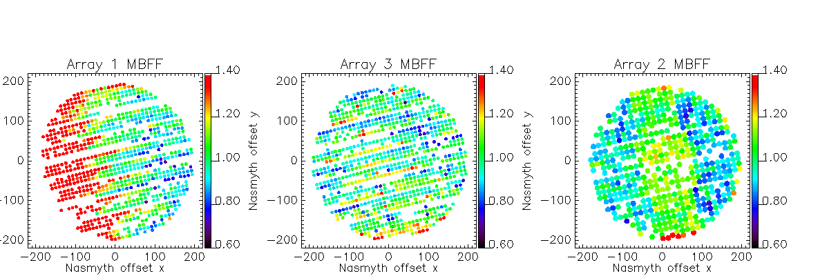
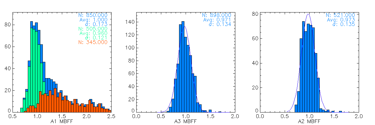
Figure 11: Average main beam flat fields obtained by combining the flat fields of five beammap scans. The top row plots show the normalized average flat fields of Array 1, 3 and 2, respectively. The offset positions with respect to the center of the array are given in arcsecond in the Nasmyth coordinate system. The colour code gives the value of the KID calibration coefficients, as defined in Eq. 20, normalized by the average calibration coefficient over all the KIDs of the array. The bottom plots show the average flat field distributions using all KIDs (blue), using Array 1 KIDs that are positioned out of the shadow zone (green) and using Array 1 KIDs inside the shadow zone, which is defined in the text.

The dispersion of the detector responsivity across the field of view (a. k. a. flat fields) has been characterized in the following ways.

Main beam flat fields. These are the focal plane distribution of the calibration coefficients per KID. They describe the focal plane distribution of the point spread function (PSF) in the far field of the telescope. The calibration coefficients $G_{k}$ are estimated using Eq. 20, as discussed in Sect. 8.1.4.

Forward beam flat fields. These are the focal plane distributions of the relative response of each KID to the near field atmospheric background. They are estimated using the correlation factor of each detector TOI to a median common mode estimated off-source (see Sect. 4.4 for more details on common modes).

Figure 11 shows the average main beam flat field for the three arrays. These have been constructed by combining the normalized flat fields of five beammaps acquired during two technical observation campaigns. These data were selected by thresholding the line-of-sight opacity measured in the 1 mm band to $\tau_{\nu}\,x\leq 0.85$. The distributions for the average flat fields are shown in the bottom panel of Fig. 11.

We observe a significant variation of the flat fields for A1 from the left-most side to the right-most side of the FOV. This reveals a significant change of A1 detector responsivities depending on their position in the focal plane. Namely, this effect mainly impacts the left-most third of the array, which is referred to as the ”shadow-zone”. This variation of the flat field translates into a broadening of the distribution shown in the lower panel of Fig. 11. However, we verified that A1’s flat field dispersions are in line with the ones of A3 after the detectors within the shadow-zone were flagged out using a crescent-shaped mask. The masked flat field distributions are shown in green in Fig. 11, whereas shadow-zone distributions are in red. The same FOV patterning is also observed in the forward beam flat fields, which excludes a main beam related issue.

The shadow zone effect is caused by a misbehaving of the dichroic in the polarized transmission which is out of specifications. As a result, the $1\,\rm{mm}$ polarisation that illuminates A1 is attenuated. This effect, which implies a dependence of the frequency cut-off on the radiation incidence angle and linear polarisation, was reproduced using optical simulations. Furthermore, this hypothesis was verified using observations at the technical campaign of September 2018. During this test campaign, a new hot-pressed dichroic had been installed in place of the current air-gap dichroic. The shadow zone variations of the flat field for A1 were not observed during the September 2018 campaign, while huge distortions across the field of view of A2 were reported. These distortions are due to the bending of the hot-pressed dichroic at low temperature. This test has confirmed that the shadow zone effect was due to incoming radiation absorption by the current air-gap dichroic. Further efforts are currently conducted to the design of a dichroic that combines robustness against bending induced by low temperature and optimal transmission. The air-gap dichroic, which is immune to low temperature-induced deformation, has been re-installed at the end of the September 2018 run coming back to the instrumental set up discussed in this paper. We have checked that, as expected, the performance of the instrument after this intervention was consistent with the one reported in this paper.

8.3 The temperature-induced variation effect

We evidenced a daily variation of the flux density estimates that correlates to the measured beam size. This beam broadening happens mostly in afternoons and around sunrise and sunset. It is also reproducible from one campaign to another. It most certainly comes from the combination of two different effects.

First inhomogeneous solar illumination leads to large scale deformations of the 30-$\rm{m}$ primary mirror, which in turn lead to variable de-focussing of the telescope. To mitigate this effect, the telescope is equipped with an active thermal ventilation system of the primary mirror and an active temperature control of the secondary support legs. This system is, however, challenged when the Sun partially illuminates the telescope This is a known effect that also impacts observations with the heterodyne instruments operated at the IRAM 30-$\rm{m}$ telescope. It had also been already observed with the previous generation total-power instruments MAMBO-2 (Kreysa et al., 1999). However, the magnitude of this effect is likely to have increased with the slow disappearance of the surface painting of the primary mirror in the past few years.

Second, on short time scales, atmospheric anomalous refraction also often plays a role.. As far as the 30-$\rm{m}$ telescope is concerned, it has first been described in Altenhoff et al. (1987). Based on experience with the heterodyne receivers, afternoon hours are often affected with an unstable atmosphere when rising moist air moves through the beam of the telescope and causes random refraction. The pointing is then observed to change within few seconds by few arcseconds resulting in an average enlargement of the beam pattern. This effect has been confirmed by measuring several arcsec displacements of the source position when projected using different subsets of subscans of a single observation, as described in Appendix C.2. We find that the apparent beam broadening during the afternoon is due to anomalous refraction for between one third and one half of the scans over the period studied here.

As both effects (the primary mirror deformations and the anomalous refraction) are due to ambient temperature variations, we refer to them as temperature-induced variation effects in the following.

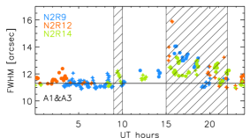
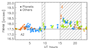
Figure 12: Beam size monitoring using OTF raster scans. Geometrical FWHM at $1\,\rm{mm}$ (top panel) and $2\,\rm{mm}$ (bottom panel), as a function of the observation time in UT hours, are shown using scans of giant planets (filled circles) and bright point-like sources with a flux density higher than $1\,\rm{Jy}$ (filled stars) for the three reference observation campaigns (N2R9,N2R12 and N2R14). The cross-hatched areas correspond to the observing time periods that are discarded using the baseline scan selection, as described in Sect. 4.6.

The temperature-induced variation of the beam size as a function of the UT hours is shown in Fig. 12 for the three reference campaigns using bright sources. These are selected by thresholding the flux density estimates above $1\,\rm{Jy}$ at both wavelengths. The beam size is estimated by fitting a 2D elliptical Gaussian to the map and computing the geometrical FWHM using Eq. 4. For the resolved planet as Uranus, the FWHM estimates are corrected for the beam broadening due to the finite extension of the apparent disc of the planet, as in Sect. 6.2. We observe the same evolution of the FWHM for all campaigns. This goes from a plateau at a median value of $11.3^{\prime\prime}$ at $1\,\rm{mm}$ and $17.5^{\prime\prime}$ at $2\,\rm{mm}$ during the night, to a smooth rise that reaches a maximum of about $14^{\prime\prime}$ at $1\,\rm{mm}$ and $18.5^{\prime\prime}$ at $2\,\rm{mm}$ around 16:00 UT hours. The beam broadening becomes large around 15:00 UT and returns to the plateau only around 22:00 UT. To mitigate the impact of the temperature-induced variation, observation scans acquired during this time interval must be discarded. The UT ranges that are discarded using the baseline scan selection (see Sect. 4.6) are shown as cross-hatched areas in Fig. 12. They consist of the afternoon period between 15:00 and 22:00 UT as well as the period from 9:00 UT to 10:00 UT while the Sun rises. Whereas the global trend of the beam variations is the same for all campaigns, we observe some variability in the amplitude of the effect over the campaigns. This supports the assumption of the important role of the partial illumination of the primary mirror by direct sun light in the temperature-induced effect. This in turn induces a variability of the amplitude of the effect depending on the angle between the telescope bore-sight and the Sun all along the observations.

The same beam size variations in time are observed using scans of giant planets (Uranus and Neptune) or other bright sources (mainly quasars). However, planets lead slightly larger FWHM estimates than quasars, because of the larger contribution of the error beams to the fitted 2D Gaussian, as their flux are measured with a higher signal-to-noise.

8.4 Baseline calibration

To assess NIKA2 performance, we rely on a baseline calibration that resorts to the following steps: i) the calibration in FWHM₀ Gaussian as detailed in Sect. 8.1 is implemented, ii) the effect of the temperature-induced variation of the beam size is mitigated using the baseline scan selection described in Sect. 4.6 and iii) the atmospheric attenuation is corrected using the corrected skydip opacity estimation described in Sect. 7.1.4.

The baseline calibration is validated below by checking the stability of Uranus flux density estimates against the beam size (Sect. 8.4.1) and against the atmospheric transmission (Sect. 8.4.2). The baseline calibration results are compared on alternative calibration methods using other opacity correction (Sect. 8.4.3).

8.4.1 Flux stability against the beam size

We present the Uranus measured-to-predicted flux density ratio as a function of the 2D Gaussian FWHM estimates and colour-coded from the observation times given in UT hours in Fig. 13. As expected from the discussion in Sect. 8.3, the largest FWHMs are measured on scans acquired in late afternoon, especially from 16:00 UT to 21:00 UT.

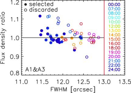
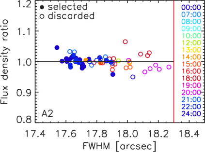
Figure 13: Uranus flux density ratio vs beam size after baseline calibration. The ratio of Uranus measured flux densities to expectations as a function of the measured 2D Gaussian beam FWHM is shown for the $1$-mm array combination (top panel) and for array 2 (bottom panel) after absolute calibration using the baseline method. These plots include all Uranus scans acquired during the N2R9, N2R12 and N2R14 campaigns and whose beam FWHMs are below the threshold indicated by the vertical red lines (open circles), as well as the scans that met the baseline selection criteria (filled circles).

The flux density estimates have been calibrated beforehand, so that the flux density ratios are equal to unity in average by construction. We observe no significant dependence of the selected scan flux ratios (shown as filled circles in Fig. 13) on the beam FWHM. This gives a first indication of the efficiency of the baseline scan selection to mitigate the temperature-induced beam variation effect. The flux stability against the beam FWHM is further assessed in Sect. 9.

8.4.2 Flux stability against the atmospheric transmission

We test the stability of Uranus flux densities calibrated using the baseline method against the atmospheric transmission. The latter depends on the measured zenith opacity $\tau_{\nu}$ and the scan average air mass x as $\exp{(-\tau_{\nu}\,x)}$. In the first row of Fig. 14, Uranus flux ratio is shown as a function of the atmospheric transmission for the $1$-mm array combination and Array 2 and for the three reference observation campaigns (N2R9, N2R12 $\&$ N2R14). We observe no significant correlation of the flux ratio with the atmospheric transmission, which gives a first indication of the robustness of the flux density estimates against the atmospheric conditions using the baseline calibration. This will be further tested using a larger number of scans towards other sources in Sect. 9.

\begin{overpic}[clip={true},trim=0.0pt -8.5359pt -8.5359pt 0.0pt,width=212.47617pt]{Figures/plot_flux_density_ratio_obstau_uranus_corrected_skydip_narrow_1mm.pdf} \put(20.0,23.0){\footnotesize Baseline} \end{overpic}

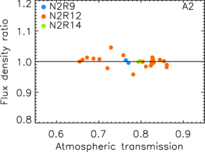
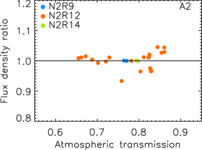
\begin{overpic}[clip={true},trim=0.0pt -8.5359pt -8.5359pt 0.0pt,width=212.47617pt]{Figures/plot_flux_density_ratio_obstau_uranus_tau225_narrow_1mm.pdf} \put(20.0,23.0){\footnotesize Taumeter} \end{overpic}

\begin{overpic}[clip={true},trim=0.0pt -8.5359pt -8.5359pt 0.0pt,width=212.47617pt]{Figures/plot_flux_density_ratio_obstau_uranus_skydip_narrow_1mm.pdf} \put(20.0,23.0){\footnotesize Skydip} \end{overpic}

Figure 14: Uranus flux density ratio vs atmospheric transmission shown for the $1$-mm array combination (left column) and for array 2 (right column) after absolute calibration using (first row) the baseline method, (second row) the ’taumeter’-based and (third row) the ’skydip’-based methods. These plots include all Uranus scans acquired during N2R9, N2R12 and N2R14 campaigns.

8.4.3 Comparison with other opacity correction methods

As a cross-check we have derived the absolute calibration factors using the taumeter (Sect. 7.1.1) and the skydip (Sect. 7.1.2) atmospheric opacity correction methods. We then compare Uranus flux density estimates after absolute calibration using the baseline calibration and these two alternative corrections. Figure 14 shows the Uranus measured-to-modelled flux ratio as a function of the atmospheric transmission for A1$\&$A3 and for A2 after the taumeter correction (second row) and after the skydip correction (third row). We observe more dispersion for the taumeter-based flux ratio, whereas the skydip-based ratio is very similar as the baseline ratio except for a slight decrease of the flux at low atmospheric transmission. Thus the taumeter and skydip atmospheric opacity correction methods can be used for the absolute calibration in complement to corrected skydip, e.g. to perform robustness tests as in Sect. 9.

9 Photometry & Stability Assessment

NIKA2 photometric capabilities after the calibration presented in Sect. 8, are assessed in this section. Firstly, we use observation of secondary calibrators (planetary nebulae NGC7027, CRL2688, and MWC349A) to test the consistency of the flux density estimates with expectations. The flux density expectations in NIKA2 bands for these calibrators are given in Appendix A.2. Then, we verify the stability of the photometry with respect to the atmospheric conditions using a large amount of observations towards a large variety of point-like sources.

The quality criteria used to assess the photometric capabilities and calibration results are defined in Sect. 9.1. In Sect. 9.2, these criteria are evaluated for the baseline calibration, and in Sect. 9.3, we compare these results with other calibration method results before summarizing the main results in Sect. 9.4.

9.1 Calibration accuracy and uncertainty assessment

We assess the photometric performance by evaluating two quality criteria: first, the calibration bias checks the accuracy of the absolute calibration and then the point-source rms calibration uncertainties test the stability of the flux densities. The stability of the full beam pattern at large angular scales, which impacts the stability of the diffuse emission flux density, is not tested here. Finally, we review here the systematic uncertainties on the flux density.

9.1.1 Calibration bias

We define the calibration bias $b_{\nu}$, where $\nu$ stands for Array 1, 2, 3 and the $1\,\rm{mm}$ array combination, as the ratio between the measured flux density $\hat{S}_{\nu}$ using the reference photometry (Sect. 8.1.1) and the flux density expectations $S_{\rm{s}}(\nu_{0})$ as given in Appendix A.2. From a series of secondary calibrator scans, we evaluate the average calibration bias $b_{\nu}$, which by construction, should be equal to unity within uncertainties. Moreover, we check the stability of the calibration bias against the observed opacities as a robustness test of the opacity derivation method. Likewise, we verify that the photometry is insensitive to optical variations by checking the stability of the calibration bias against the measured beam size.

9.1.2 Point-source rms calibration uncertainties

We evaluate the standard deviation of bright point-like source measured-to-median flux density ratio $\sigma_{\nu}$ per array or array combination $\nu$. As the flux density of most of the considered sources is unknown a priori, we compare the flux density estimate in a single observation scan to the average flux density throughout an observation campaign. This method requires the selection of sources that are bright enough to be detected with a high signal-to-noise ratio with a single repetition of an usual $8^{\prime}\times 5^{\prime}$ OTF raster scan. Namely, we perform a source selection by setting a threshold on the flux estimate to $800\,\rm{mJy}$ at $1\,\rm{mm}$ and $400\,\rm{mJy}$ at $2\,\rm{mm}$. Moreover, we consider only the sources for which a minimum of $10$ scans are available after selection to ensure a precise average flux density estimation. Finally, the selected source scans must meet the baseline scan selection criteria given in Sect. 4.6.

Since the flux density ratios are not Gaussian distributed, we evaluate the 68 and 95% confidence level (C.L.) contours using the measured distributions in order to further characterise the uncertainties. We check that the rms errors are larger than the 68% C.L. contours and thus provide conservative $1\sigma$-like errors.

As the rms of the flux density ratio is estimated on a scan set that is representative of the observing conditions encountered at the 30-$\rm{m}$ telescope, this is an estimate of the calibration uncertainties that encloses errors of optical, atmospheric, instrumental noise and data processing origins. This includes the errors sourced by the temperature-induced beam variations, the effect of the elevation, the uncertainties of the atmospheric opacity correction using either the skydip or the taumeter method and the atmospheric and instrumental noise residuals after the data reduction (Sect. 4). However, as the data set comprises point-like sources and because flux density measurements in the reference photometric system are immune to beam variations at large angular scales, we refer to the rms of the flux density ratios as point-source rms calibration uncertainties.

For extended sources and diffuse emission studies, the maps in Jy/beam units, where the beam refers to the reference beam, are converted into Jy/sr units using Eq. 19. Propagating the uncertainty on the total beam solid angles, the reference beam efficiencies are estimated with a precision of 5$\%$ and 3$\%$ at 1 and 2 mm, respectively, as reported in Table 13 in Sect. 8.1.3. These uncertainties must be further accounted for in the error budget of diffuse emission studies.

\begin{overpic}[clip={true},trim=25.6073pt 5.69046pt 0.0pt 17.07182pt,width=230.68483pt]{Figures/plot_flux_density_ratio_MWC349_obstau_corrected_skydip_narrow_1mm.pdf} \put(20.0,60.0){\footnotesize{\tt Baseline}} \end{overpic}

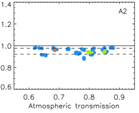
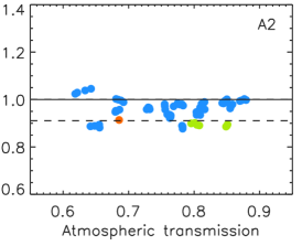
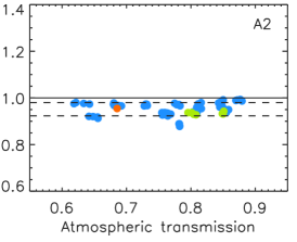
\begin{overpic}[clip={true},trim=25.6073pt 5.69046pt 0.0pt 17.07182pt,width=230.68483pt]{Figures/plot_flux_density_ratio_MWC349_obstau_tau225_narrow_1mm.pdf} \put(20.0,60.0){\footnotesize{\tt Taumeter}} \end{overpic}

\begin{overpic}[clip={true},trim=25.6073pt 5.69046pt 0.0pt 17.07182pt,width=230.68483pt]{Figures/plot_flux_density_ratio_MWC349_obstau_skydip_narrow_1mm.pdf} \put(20.0,60.0){\footnotesize{\tt Skydip}} \end{overpic}

\begin{overpic}[clip={true},trim=25.6073pt 5.69046pt 0.0pt 17.07182pt,width=230.68483pt]{Figures/plot_flux_density_ratio_MWC349_obstau_corrected_skydip_photocorr_demo_narrow_1mm.pdf} \put(20.0,60.0){\footnotesize{\tt PC-demo}} \end{overpic}

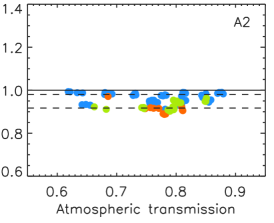
\begin{overpic}[clip={true},trim=25.6073pt 11.38092pt 0.0pt 17.07182pt,width=230.68483pt]{Figures/plot_flux_density_ratio_MWC349_obstau_corrected_skydip_photocorr_pointing_narrow_1mm.pdf} \put(20.0,60.0){\footnotesize{\tt PC-point}} \end{overpic}

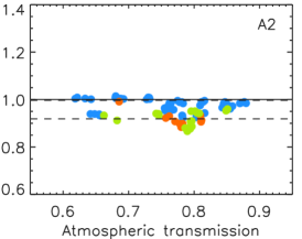
Figure 15: Comparison of the calibration bias for five calibration methods using observations of MWC349. The measured-to-expected flux density ratio is shown as a function of the atmospheric transmission for the baseline method (first row) as well as for methods using the taumeter (second row) and skydip (third) opacity correction, and for methods resorting to the PC-demo (fourth) and PC-point (fifth) photometric corrections. Dashed lines show the flux density ratio rms errors.

9.1.3 Absolute and systematic uncertainties

To account for all uncertainties, we must add to the point-source rms calibration uncertainties the absolute calibration uncertainties and the systematic errors. The absolute uncertainty is the uncertainty on the primary calibrator flux density expectations. In the case of Uranus, Moreno (1998) and Bendo et al. (2013) report uncertainties of about $5\%$ at both wavelengths.

For the baseline calibration method, which resorts to the corrected skydip method for the atmospheric opacity correction (see Sect. 7.1.4), the uncertainties on the correcting factor $a_{\nu}^{\rm{skydip}}$, as defined in Eq. 14, must be propagated to the flux uncertainties. These uncertainties, which are referred to as the corrected skydip uncertainties, depend on the line-of-sight atmospheric opacity $\tau_{\nu}x$. Precisely, because the corrected skydip opacity correction is consistently used for both the primary calibrator and the target source flux measurement, the corrected skydip uncertainties depends on the difference between the average line-of-sight opacity of the primary calibrator scans and the line-of-sight opacity of the source scan. We evaluate the corrected skydip uncertainties for two different $\tau_{\nu}x$ values. 1) For the reference IRAM 30-$\rm{m}$ winter observing conditions, defined as $2\,\rm{mm}$ of pwv and an elevation of $60^{\rm{o}}$, the corrected skydip uncertainties are of 0.6% at $1\,\rm{mm}$ and 0.3% at $2\,\rm{mm}$. 2) In the worst observing conditions allowed by the baseline scan selection (Sect. 4.6), which are $\tau_{\nu}x$ of 0.7 at $1\,\rm{mm}$ and of 0.5 at $2\,\rm{mm}$, we find corrected skydip uncertainties of 2% and $1.5\%$ at 1 and $2\,\rm{mm}$, respectively. These constitute conservative upper limits on the corrected skydip uncertainties.

The uncertainties on NIKA2 bandpass measurements (see Sect. 2.5) propagate into uncertainties on the flux densities after the colour correction using Eq. 18. These uncertainties depend on the source SED but are negligible in most of the cases. In particular, for MWC349, we find uncertainties below 0.1% at both wavelengths.

9.2 Baseline calibration photometry results

We measure the calibration bias and rms uncertainties, as defined in the previous section (Sect. 9.1) using the baseline calibration method (Sect. 8.4).

The calibration bias is evaluated using a series of scans of MWC349 acquired during the reference observation campaigns. Namely, we use the 72 scans that met the baseline selection criteria (see Sect. 4.6) over the 109 available scans for MWC349. The first row of Fig. 15, labelled ’baseline’, shows the calibration bias $b_{\nu}$ for the combination of the $1\,\rm{mm}$ arrays and Array 2 as a function of the atmospheric transmission $\exp\left(-\tau_{\nu}\,x\right)$. No significant dependency of the calibration bias on the atmospheric transmission is observed.

Table 14 gathers the calibration bias estimates for the three observation campaigns and for all the scans. In the $1\,\rm{mm}$ band, we find $b_{\nu}$ in agreement with unity within the statistical dispersion for the three campaigns, whereas a $5\%$ lack of flux with respect to expectations is observed at $2\,\rm{mm}$, consistently for the three campaigns. This bias has a low significance with respect to the absolute calibration precision of NIKA2 (see Sect. 9.1). This will be further investigated by using other calibration methods in Sect. 9.3.

Table 14: Baseline calibration results: photometry accuracy and uncertainties. The first sub-panel labelled ’Bias’ gives the calibration bias $b_{\nu}$ and the second sub-panel labelled ’Rms’ the calibration rms error $\sigma_{\nu}$, as defined in Sect. 9.1, using observations during N2R9, N2R12, N2R14 and the combination of the three campaigns. In each sub-panel, the first row indicates the number of acquired scans, while the second row gives the number of selected scans using the baseline scan selection.

Characteristics		N2R9	N2R12	N2R14	Combined
Bias	$\#$ total	68	14	27	109
	$\#$ selected	64	1	7	72
	A1	0.95	1.03	0.94	0.95
	A3	0.99	1.07	1.00	1.00
	1mm	0.97	1.05	0.97	0.98
	2mm	0.95	0.95	0.93	0.95
Rms	$\#$ total	303	72	112	487
$[\%]$	$\#$ selected	219	33	12	264
	A1	5.7	4.6	2.9	5.5
	A3	6.2	5.7	2.4	6.0
	1mm	5.9	5.0	2.5	5.7
	2mm	3.2	2.1	1.1	3.0

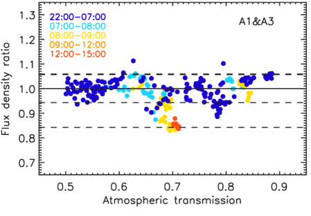
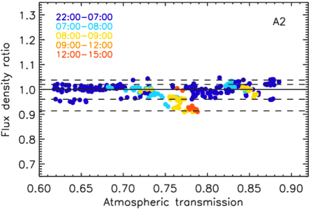
Figure 16: Baseline rms calibration uncertainties. The measured-to-median flux density ratio of bright sources is plotted as a function of the atmospheric transmission colour-coded according to the UT observation time of the scans for the combination of A1$\&$A3 (top panel) and for A2 (bottom panel). The inner dashed lines from either sides of the unity-ratio line show the rms errors, which are less than 6% at $1\,\rm{mm}$ and 3% at $2\,\rm{mm}$, while the outer dashed lines show the $95\%$ confidence level contours. The lowest flux ratio data points correspond to some of the scans acquired during daytime between 8:00 UT and 15:00 UT hours (yellow and red), while the scans acquired during night-time between 22:00 UT and 7:00 UT yield data points (dark blue) well distributed within the rms error with a few outliers.

Figure 16 shows the measured-to-median flux densities evaluated from bright source scans for the combination of Array $1\&3$ and Array 2 as a function of the atmospheric transmission and colour-coded as a function of the observation time. From a total of 487 scans towards flux-selected sources, acquired during N2R9, N2R12 and N2R14, 264 met the baseline selection criteria and are included in Fig. 16 for testing the calibration stability. The calibration uncertainties are estimated using the standard deviation of the flux density ratios for the three campaigns. Results are gathered in Table 14. Combining all the scans, we find rms uncertainties of $5.5\%$ for A1, $6.0\%$ for A3, $5.7\%$ for the $1\,\rm{mm}$ band and $3.0\%$ for A2. Using the flux ratio distributions, we construct the 68 and 95% C.L. intervals. The 68% C.L. intervals are $-6.4\%$ and $+3.4\%$ at $1\,\rm{mm}$ and $-3.8\%$ and $+1.5\%$ at $2\,\rm{mm}$. Hence in average the 68% C. L. errors are of $4.9\%$ and $2.7\%$ at 1 and $2\,\rm{mm}$, respectively. We conclude that the rms errors are conservative estimates of the 68% C. L. errors at both wavelengths. The 95% C.L. contours are $-15.8\%$ and $+5.9\%$ at $1\,\rm{mm}$ and $-8.6\%$ and $+3.8\%$ at $2\,\rm{mm}$. The rms errors and the 95% C.L. interval are shown in Fig. 16 with the inner and outer dashed lines, respectively.

The flux density ratio is constant within the rms errors along the wide range of tested atmospheric transmission, ranging from 0.5 to 0.9 at $1\,\rm{mm}$. However, some scans at atmospheric transmissions of about 0.7 at $1\,\rm{mm}$ show a mild lack of flux density with respect to the median within the 95% C. L. contours. The scans affected by the lack of flux have all been observed either between 12:00 and 14:00 UT or between 8:00 and 9:00 UT, that are close to the threshold of the observation time cuts of the baseline scan selection (see Sect. 4.6). These scans are likely to be affected by the temperature-induced beam broadening or by the sunrise focus drift, respectively. Furthermore, we find that restricting the used observation time to the 10 more stable hours (from 22:00 to 08:00 UT) would result in rms calibration uncertainties of $3.6\%$ at $1\,\rm{mm}$ and $1.2\%$ at $2\,\rm{mm}$, which constitute an improvement of about $60\%$ at $1\,\rm{mm}$ and $40\%$ at $2\,\rm{mm}$ of the rms errors. The baseline scan selection, which i) retains 16 hours of observation time a day and ii) results in state-of-the-art rms calibration uncertainties, constitutes an useful trade-off representative of most of the observations with NIKA2.

9.3 Comparison with other calibration methods

Table 15: Comparison of results using five calibration methods: (first column) the baseline calibration, (second and third) the calibration methods using other opacity correction, taumeter and skydip, respectively, and (fourth and fifth) the calibration methods using a photometric correction, PC-demo and PC-point, respectively (see Appendix C). The calibration biases, as defined in Sect. 9.1.1, are reported in the sub-panel labelled ’Bias’. The sub-panel labelled ’Rms’ gathers (first row) the total number of observation scans of bright sources (see Sect. 9.1.2) acquired during the reference campaigns, (second row) the number of selected scans, and (third to sixth rows) the rms calibration uncertainties (Sect. 9.1.2) for Array 1, Array 3, the combination of A1 and A3, and Array 2, respectively.

		Methods
Characteristics		baseline	taumeter	skydip	PC-demo	PC-point
Bias	A1	0.95	0.98	0.97	0.95	0.97
	A3	1.00	1.02	1.02	0.99	1.00
	1mm	0.98	1.01	1.00	0.97	0.99
	2mm	0.95	0.95	0.95	0.95	0.95
Rms	$\#$ total	487	487	487	396	396
$[\%]$	$\#$ selected	264	264	264	291	283
	A1	5.5	7.5	7.3	4.0	4.9
	A3	6.0	8.1	7.1	4.1	5.2
	1mm	5.7	7.9	7.1	3.8	4.9
	2mm	3.0	3.8	3.0	2.2	2.4

In this section, the baseline calibration results are compared to results drawn either using other calibration methods obtained from different opacity corrections (taumeter and skydip as discussed in Sect. 8.4.3), or including a photometric correction (PC-demo and PC-point, as described in Appendix C) to mitigate the temperature-induced variation effect (Sect. 8.3). For robustness test, we evaluate and compare the photometry quality criteria of Sect. 9.1 for the five calibration methods.

9.3.1 Calibration bias

We present the calibration bias as a function of the atmospheric transmission for the five calibration methods in Fig. 15 and report the results in the row labelled ’Bias’ of Table 15.

At $1\,\rm{mm}$, all methods lead to flux density estimates in agreement with expectations within the rms dispersion. However, taumeter flux ratios have more dispersion than the baseline flux ratios whereas skydip shows some dependency on the atmospheric transmission, with a 10 to $15\%$ excess of the flux density with respect to expectations at high transmission. This residual systematic effect has motivated the development of the corrected skydip method, as discussed in Sect. 7.1.4. These features, which are already noticeable from Fig. 15, will be confirmed and further discussed later using more observation scans. On the other hand, the calibration methods based on photometric correction (Appendix C) yield an unbiased photometry (calibration bias in agreement with unity within the rms error) while allowing the use of $30\%$ more scans. These results are encouraging for the exploitation of scans acquired during the observing periods impacted by the temperature-induced beam variation effect (Sect. 8.3).

At $2\,\rm{mm}$, all methods result in a similar calibration bias of $0.95$ with a rms error of $0.05$ estimated on the MWC349 scans. This corresponds to a low-significance $5\%$ lack of flux density towards MWC349. To summarize, the calibration bias at $2\,\rm{mm}$ is stable against i) a large range of atmospheric conditions, ii) the observation campaign, iii) the opacity correction method, iv) the method to treat the temperature-induced beam variation effect. This $5\%$ lack of flux density is thus probably due to uncertainties on the flux density expectations for this source. They come in two flavours. Firstly the uncertainties on the flux expectation, as reported in Appendix A.2, consist in the propagation of the errors on the fitted SED from the Plateau de Bure Interferometre (PdBI) and the Very Large Array (VLA) observations. Systematic uncertainties that may also impact the SED are not included. Secondly, the NIKA2 flux density extrapolation from interferometer data may be not straightforward for MWC349. In particular, NIKA2 flux extrapolation ignores the contamination by strong masers in the radio recombination lines (Gordon, 1994), while strong maser emission lines are masked in PdBI observations to measure the continuum. In addition, the resulting continuum shows indications of variability.

9.3.2 Calibration rms uncertainties

The calibration rms uncertainties for the five methods evaluated using flux-selected source scans are gathered in the sub-panel labelled ’Rms’ of Table 15.

Compared to the baseline method, the taumeter method leads to rms errors increased of about $40$ and $30\%$ at 1 and $2\,\rm{mm}$, respectively. The skydip method shows lower dispersion but a mild correlation with the atmospheric transmission, as discussed in Sect. 9.3.1.

In addition, we have checked the flux density ratios for the bunch of scans with an atmospheric transmission of about 0.7, which were discussed in Sect. 9.2, by comparing calibration methods with or without photometric correction. The flux density ratios are low (within the 95% C.L. interval) for the scans observed within 12:00 and 15:00 UT in the three first methods, as shown in Fig. 16 for the baseline method. By contrast, they are within the 68% C.L. interval when using a photometric correction. This further validates the hypothesis that the low flux density of these scans is due to temperature-induced beam effect, as assumed in Sect. 9.2. This also constitutes an example of the calibration improvement obtained by using a photometric correction.

Moreover, results based on the PC-demo method show that rms calibration uncertainties as low as $3.8$ and $2.2\%$ at 1 and $2\,\rm{mm}$ are within the reach of NIKA2 without any selection based on the observation time. However, we recall this method relies on accurate beam estimates. Using PC-point, which is the practical case, still improves the calibration uncertainties w.r.t. the baseline results but by a factor of about $20\%$ in both bands. Furthermore, the differences between the flux density ratios from PC-demo and PC-point, which are seen e.g. from the corresponding panels of Fig. 15, are likely to be due to the photometric correction noise when monitoring the beam from pointing scans (see Appendix C.2). We conclude that more control on the beam monitoring is needed before routinely using a calibration based on photometry correction. By contrast, the baseline method combines good performance with robustness.

9.4 Summary

Among the methods that rely on the UT hour-based scan selection to mitigate the effect of beam size variations, the baseline method shows the best performance in terms of calibration bias and uncertainties. The methods that rely on a photometric correction show good calibration results, and thus represent a promising lead to further improve the calibration uncertainties. However, their robustness depends on the accuracy of the beam monitoring. The proposed beam monitoring based on pointing scans induces some extra dispersion of the flux densities. A more accurate beam monitoring is feasible but requires using dedicated observation scans. From the baseline method results discussed in Sect. 9.2, we have found that the measured flux density of MWC349 is in agreement with expectations within $5\%$ for both wavelengths. Moreover, the point-source rms calibration uncertainties are of $5.7\%$ at $1\,\rm{mm}$ and of $3\%$ at $2\,\rm{mm}$ using a series of 264 scans of sources of flux density above $1\,\rm{Jy}$. These results demonstrate the excellent accuracy and stability of the NIKA2 point-source photometric capabilities.

10 Sensitivity

In this section, we derive the on-sky sensitivity of the instrument using a large amount of observation scans, including deep integration on faint sources, and assess the stability of our results against the observing conditions. We evaluate the noise equivalent flux density, which is referred to as NEFD hereafter. To further represent the mapping capabilities, we also derive the mapping speed. We first discuss the definitions and the technical derivation of these quantities in Sect.10.1 from measurements. Then, we briefly present several estimation methods that have been considered and the data sets that have been selected in Sect. 10.2. Results, together with robustness tests, are reported in Sect. 10.3.

10.1 NEFD and mapping speed definitions

The NEFD is the $1\,\sigma$ error on the flux density of a point source in one second of integration time, considered at zero atmospheric opacity. At this stage, we consider a map of a point-like source located at its center and observed with zero atmospheric opacity. The estimation of the flux density uncertainty $\sigma$ is described in Sect. 4. We derive here the integration time from actual observations. Indeed, it is not simply the duration of a scan, it depends on the KID distribution in the FOV and the scanning strategy. The flux density map, which has a resolution of $\Delta r$, also comes along with a hit map $H_{\rm{p}}$, which counts the number of data samples per pixel (see Sect. 4). From this, we derive the integration time at the center of the map as

$$t_{\rm{center}}=\frac{\langle H_{\rm{p}}\rangle_{\rm{center}}}{f_{\rm{sam}}}\,,$$ (21)

where $f_{\rm{sam}}$ is the sampling frequency and $\langle H_{\rm{p}}\rangle_{\rm{center}}$ is the average of the hit map taken in a disk of radius of one FWHM to be immune to shot noise statistics in individual map pixels. Correcting this quantity from the density of detectors per map pixel at the same time, gives the on-source integration time per beam, in other words, the time when the source is actually being observed, by at least one detector:

$$t_{\rm{beam}}=t_{\rm{center}}\,\frac{g^{2}}{\Delta r^{2}}\,,$$ (22)

where $g$ is the center-to-center distance between adjacent KIDs in the FOV (Sect. 5.2). $t_{\rm{beam}}$ matches the total duration of the scan if the scanning strategy is designed so that the source is always in the FOV and if the FOV is full of valid KIDs. The NEFD is defined using the previous quantities as

$$\rm{NEFD}=\sigma\sqrt{t_{\rm{beam}}}\,$$ (23)

and is given in $\rm{mJy}\cdot s^{1/2}$.

The mapping speed, $M_{\rm{s}}$, is the sky area $\mathcal{A}_{\rm{scan}}$ that can be mapped at a noise level $\Delta_{\sigma}$ of $1\,\rm{mJy}$ in an integration time $\Delta_{t}$ of one hour. Noting $d_{\rm{FOV}}=6.5\,\rm{arcmin}$ the FOV diameter and $\eta$ the fraction of valid KIDs for an observation (Sect. 5.1), the mapping speed is

$$M_{\rm{s}}=\frac{\mathcal{A}_{\rm{scan}}}{\Delta_{\sigma}\Delta_{t}}=\eta\,\frac{\pi}{4}d_{\rm{FOV}}^{2}\,\frac{1}{\rm{NEFD}^{2}}\,,$$ (24)

and has units of arcmin${}^{2}\cdot\rm{mJy}^{-2}\cdot\rm{h}^{-1}$. In real observation conditions, characterized with a given atmospheric opacity $\tau_{\nu}$ and a given air mass $x$, correcting the flux density for atmospheric attenuation using Eq. 8 increases the NEFD as

$$\rm{NEFD}_{\tau_{\nu},\,x}=\rm{NEFD}\,e^{\tau_{\nu}x}$$ (25)

Using these definitions, the integration time required to reach a target flux density uncertainty $\sigma_{obs}$ over an observing area $\mathcal{A}_{\rm{scan}}$ for an airmass $x$ and for an atmospheric opacity $\tau_{\nu}$ is

$$t_{\rm{obs}}=\frac{\mathcal{A}_{\rm{scan}}}{M_{\rm{s}}}\,\left(\frac{e^{\tau_{\nu}\,x}}{\sigma_{obs}}\right)^{2}.$$ (26)

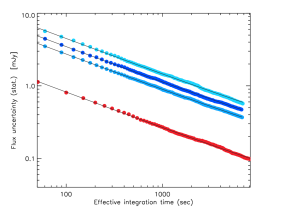
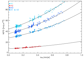
Figure 17: Comparison of NEFD estimates using two methods on observations of HLS J0918+5142. Left panel: Evolution of the 1 $\sigma$ flux density uncertainties as a function of the effective integration time $t_{\rm{eff}}$, as defined in Eq. 27, for A1 (cyan), A3 (dark blue), the combination of A1&A3 (medium blue), and A2 (red). The solid black lines are the best-fit models using $\sigma(t_{\rm{eff}})=\rm{NEFD}/sqrt(t_{\rm{eff}})$. Right panel: NEFD as a function of the measured line-of-sight opacity using the same colour code as in the left panel. The solid black lines are the theoretical fits of $\rm{NEFD}_{\tau_{\nu},\,x}=\rm{NEFD}\,e^{\tau_{\nu}\,x}$ and give the NEFD when extrapolated to $\tau_{\nu}/\sin(\rm{el})=0$.

10.2 NEFD estimation methods and scan selection

We have developed several methods for the NEFD estimation. First, we use deep integrations on faint sources. Second, we resort to joint analysis of multiple scans without combining them.

10.2.1 Deep integration method

According to Eq. 23 and Eq. 25, if a source was observed under stable atmospheric conditions, the flux uncertainty would scale directly like $t_{\rm{beam}}^{-1/2}$. Using long-time integration observation on a source, this relation provides both a way to estimate the NEFD and to check that the noise does integrate down as expected with the integration time. To that aim, we produce a series of maps, as described in Sect. 4.5, using an inverse-variance co-addition of an increasing number of observation scans, and perform a photometric analysis on each map according to Sect. 9. However, in practice, in particular for integrations of several hours, observing conditions do change. Since all the scans are not acquired in the same conditions of atmospheric opacity and observing elevation, they will not need the same atmospheric opacity correction, nor have the same level of atmospheric noise residuals after the noise decorrelation, as described in Sect. 4.4, and hence, they do not contribute with the same weight to the co-addition. In such case, an effective integration time for the co-addition of $n$ scans is defined as

$$t_{\rm{eff}}(n)=\sum_{i=1}^{n}\,t_{i}\,e^{-2\tau_{\nu}^{i}\,x_{i}},$$ (27)

where $t_{i}$, $\tau_{\nu}^{i}$ and $x_{i}$ are the integration time, the zenith opacity and the air mass of the $i$-th scan of the $n$-scans co-addition. Generalizing Eq. 23, the flux density uncertainties on the co-addition of $n$ scans is $\sigma(n)=\rm{NEFD}/\sqrt{t_{\rm{eff}}(n)}$. An estimate of the NEFD can therefore be obtained in fitting $\sigma(n)$ as a function of the corresponding $t_{\rm{eff}}(n)$.

10.2.2 Scatter method

For any scan, we derive $\rm{NEFD}_{\tau_{\nu},\,x}$. Using Eq. 25, the joint analysis of a series of scans acquired with various observing conditions provides an estimate of the NEFD. The scan sample can gather different sources. The selection of the source target for the NEFD derivation is primarily based on the flux density. Indeed, noise characterization may be biased by the signal of a bright source stemming from the most extended error beams and far side lobes. We therefore restrict the analysis to sources with estimated flux below 1 Jy.

Table 16: Stability of the NEFD estimates. Top-of-atmosphere NEFD in $\rm{mJy}.s^{1/2}$ for the two methods described in the text, which are the deep integration (labelled Deep int) and the scatter method (Scatter), and using two different data sets, HLS J0918+5142 and all sub-Jy sources acquired during the reference observation campaigns. The results given in the last row are based on more than a thousand scans (202, 481 and 430 scans during N2R9, N2R12 and N2R14, respectively).

Data set	Method	A1	A3	A1&A3	A2
HLS J0918+5142	Deep int.	46.6	38.4	30.4	8.5
	Scatter	45.7	36.3	28.5	8.2
N2R9	Scatter	47.0	36.9	28.8	8.4
N2R12		47.3	36.4	30.2	8.5
N2R14		47.3	39.8	30.9	9.3
Combined		47.2	37.9	30.1	8.8

10.3 Results and robustness tests

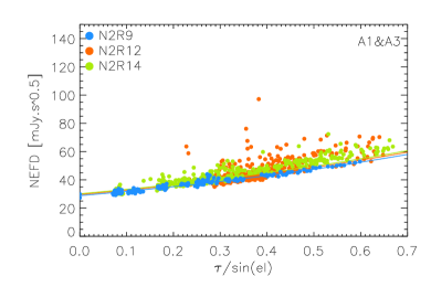
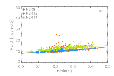
Figure 18: Comparison of the NEFD estimates for three observation campaigns. The measured NEFD using the scatter method is plotted as a function of line-of-sight opacity ($\tau_{\nu}\,x$) for the $1\,\rm{mm}$ (left) and $2\,\rm{mm}$ (right) channels. Data points are NEFD estimates in $\rm{mJy}\cdot s^{1/2}$ for N2R9 (blue), N2R12 (orange) and N2R14 (chartreuse). We also show in the plots the expected NEFD evolution with the line-of-sight opacity as solid curves using the median zenith opacity derived from all the scans acquired during a campaign.

Table 17: Median NEFD and rms uncertainties in $\rm{mJy}\cdot s^{1/2}$, as well as the derived mapping speed and mapping speed rms uncertainties in $\rm{arcmin}^{2}\cdot\rm{mJy}^{-2}\cdot\rm{h}^{-1}$, evaluated in using the scatter method on all sub-Jy sources of runs N2R9, N2R12 and N2R14, given at pwv=0 and 90 degrees elevation (first three rows) and extrapolated at the reference Winter observing conditions at the IRAM 30-$\rm{m}$ telescope site (last three rows), which are defined as $2\,\rm{mm}$ pwv and 60 degrees elevation.

	A1	A3	A1&A3	A2
NEFD  ($0\,\rm{mm}$ pwv, $90^{\rm{o}}$)	47.2	37.9	30.1	8.8
Rms NEFD  ($0\,\rm{mm}$ pwv, $90^{\rm{o}}$)	3.9	3.5	2.9	1.1
Ms  ($0\,\rm{mm}$ pwv, $90^{\rm{o}}$)	45	70	111	1388
Rms Ms  ($0\,\rm{mm}$ pwv, $90^{\rm{o}}$)	4	6	11	174
NEFD  ($2\,\rm{mm}$ pwv, $60^{\rm{o}}$)	56.6	45.6	36.1	9.8
Rms NEFD  ($2\,\rm{mm}$ pwv, $60^{\rm{o}}$)	4.7	4.2	3.5	1.2
Ms  ($2\,\rm{mm}$ pwv, $60^{\rm{o}}$)	31	48	77	1119
Rms Ms  ($2\,\rm{mm}$ pwv, $60^{\rm{o}}$)	3	4	7	137

First we test the stability of the NEFD estimates using the two methods on the same data set. With this goal, during the N2R9 run, we selected HLS J0918+5142, a moderately faint source (Combes et al., 2012), expected to have flux densities of 74.5 mJy at $1\,\rm{mm}$ and 15.7 mJy at $2\,\rm{mm}$. It was observed for about 9 h in total over three nights using $8\times 5$ arcmin² OTF raster scans of various orientations.

The left panel of Fig. 17 shows the flux density uncertainties as a function of the integration time. The effective integration time is different between the 1 mm and 2 mm arrays because they have different KID spacings $g$ in the FOV and different atmospheric opacities (see Eq. 27). Black lines show the fit with the inverse of the square root of the integration time, confirming that the noise integration is well consistent with the expected scaling law. The observed small variations around the theoretical fit correspond to variations of line-of-sight opacity during the integration. These variations are taken into account for evaluating the NEFD as discussed in the previous section. The right panel of Fig. 17 shows the $\rm{NEFD}_{\tau_{\nu},\,x}$ per scan, along with best-fit models using Eq. 25, from which are derived the NEFD estimates. Results from these analyses, per array and for the combined A1 and A3, are presented in Table 16.

We observe systematically higher NEFD for A1 compared to A3, which is a mainly due to the dichroic-induced ’shadow effect’ that also impacts the flat fields, as discussed in Sect. 8.2. The dichroic-induced effect, which also impacts A3, explains part of the NEFD difference of performance between the $1\,\rm{mm}$ and $2\,\rm{mm}$ channels, together with the higher atmospheric noise and lower telescope beam efficiency at $1\,\rm{mm}$ with respect to $2\,\rm{mm}$ wavelength. Moreover, the NEFD evolution with sky noise is well consistent with expectations for each array and each observing wavelength.

As a second robustness test, we check the stability of the NEFD for three observation campaigns. Figure 18 shows the measured NEFD using the scatter method (see Sect. 10.2) for the sub-Jansky sources acquired at the N2R9, N2R12 and N2R14 campaigns. The NEFD estimates for the three campaigns are in agreement within uncertainties for the whole range of line-of-sight opacities that have been tested. The solid lines show the expected dependence with exp${[\tau_{\nu}\,x]}$ as given in Eq. 25. Since the measured NEFD${}_{\tau,\,x}$ are not Gaussian distributed, we derive the NEFD as the median of the NEFD${}_{\tau,\,x}$ per scans after correction of the atmospheric attenuation, which provides us with a more robust estimate compared to a fit. The NEFD estimates are given in Table 16.

Combining the data set of N2R9, N2R12 and N2R14 campaigns, more than one thousand observations scans of sub-Jy sources meet the baseline selection criteria (see Sect. 4.6), providing robust NEFD estimates that are representative of the average NIKA2 performance. The rms uncertainties are evaluated as the rms scatter of the individual NEFD${}_{\tau_{\nu},\,x}$ estimates after correction with $e^{\tau_{\nu}\,x}$. These values are then extrapolated using the IRAM 30-$\rm{m}$ telescope reference Winter observing conditions: $2\,\rm{mm}$ of precipitable water vapour (pwv) and $60$ degrees elevation. The NEFD estimates, as well as the rms uncertainties, are gathered in Table 17. From these estimates, we also derive the corresponding mapping speeds, which are also given in Table 17. We report mapping speeds of $1388\pm 174$ and $111\pm 11\,\rm{arcmin}^{2}\cdot\rm{mJy}^{-2}\cdot\rm{h}^{-1}$ at 1 and 2 mm, respectively.

11 Summary and conclusions

Table 18: Summary of the main characteristics describing NIKA2 measured performance

	Array 1&3	Array 2		Reference
Reference Wavelength [mm]	1.15	2.00
Reference Frequency [GHz]	260	150		Sect. 8.1.1
Frequency [GHz]	254.7&257.4	150.9		Sect. 2.5
Bandwidth [GHz]	49.2&48.0	40.7
Number of designed detectors	1140&1140	616		Sect. 2.3
Number of valid detectors	952&961	553		Sect. 5.3
Fraction of valid detectors [$\%$]	84	90
Pixel size in beam sampling unit    [$\lambda/D$]	1.1	0.87		Sect. 5.2
FWHM    [arcsec]	$11.1\pm 0.2$	$17.6\pm 0.1$		Sect. 6.2
Main beam efficiency    [$\%$]	$47\pm 3$	$64\pm 3$		Sect. 6.3
Rms FWHM across the FOV [arcsec]	0.6	0.6		Adam et al. (2018)
Reference FWHM    [arcsec]	$12.5$	$18.5$		Sect. 8.1.1
Reference beam efficiency    [% ]	$61\pm 3$	$72\pm 2$		Sect. 8.1.3
Rms pointing error [arcsec]	$<3$	$<3$		Sect. 3.2
Absolute calibration uncertainty [%]	5	5		Sect. 9.1, App. A.1
Systematic calibration uncertainty    [%]	0.6	0.3		Sect. 9.1.3
Point-source rms calibration uncertainty [%]	5.7	3.0		Sect. 9.2
$\alpha$ noise integration in time	0.5	0.5		Sect. 10.3
NEFD    [$\rm{mJy}\cdot\rm{s}^{1/2}$]	$30\pm 3$	$9\pm 1$		Sect. 10.3
Ms    [arcmin${}^{2}\cdot\rm{mJy}^{-2}\cdot\rm{h}^{-1}$]	$111\pm 11$	$1388\pm 174$

We have presented NIKA2 performance at the IRAM 30-$\rm{m}$ telescope. It has been evaluated with a baseline calibration method that goes from observations and raw data to measured flux densities. In the baseline calibration photometric system, the flux density of point-like sources are measured as the amplitude estimates of a fixed-width Gaussian of FWHM of $12.5^{\prime\prime}$ and $18.5^{\prime\prime}$ at the $150$ and $260\,\rm{GHz}$ reference frequency, respectively.

This method relies on three main analysis choices. First the atmospheric and instrumental correlated noises are corrected using a simple and robust method based on the subtraction of a series of the average temporal signals of the most correlated detectors. The atmospheric opacity is estimated using an improved version of the method proposed in Catalano et al. (2014) and used in Adam et al. (2018), which is based on the use of NIKA2 as an in-band total-power taumeter. Finally a scan selection based on the observation time is performed and retains 16 hours of observation a day in order to mitigate the effect beam size variations due to anomalous refraction of the atmosphere and partial illumination of the 30-$\rm{m}$ telescope that mainly impact the afternoon observations. We have also considered the pros and cons of alternative methods, which may in the future lead to even better calibration accuracy and stability.

The performance of the NIKA2 camera has been assessed using a large number of observations of primary and secondary calibrators and faint sources that have been acquired during three observational campaigns over one year. The data set spans the whole range of observing elevation and atmospheric conditions encountered on-site. The main characteristics that define the NIKA2 performance are summarized in Table 18. We highlight the main points in the following.

1. All designed KIDs detect the signal at least in some observation scans. We conservatively retain only the most stable KIDs, which are immune to the cross-talking effect and yield good signal-to-noise measurement. We report valid KID fractions of $84\%$ for the $1\,\rm{mm}$ channel arrays and $90\%$ for Array 2. The other KIDs, which do not meet the validity criterion, are randomly distributed across the FOV, so that the whole $6.5\,\rm{arcmin}$ FOV is covered.

2. The main beam is well described with a 2D Gaussian of FWHM of $11.1^{\prime\prime}$ for the $1\,\rm{mm}$ channel arrays and $17.6^{\prime\prime}$ for Array 2, with uncertainties of $0.2^{\prime\prime}$ for the combination of Array 1$\&$3 and of $0.1^{\prime\prime}$ for Array 2. Comparing the main beam fit to the measured full beam, and including large angular scale contributions from IRAM 30-$\rm{m}$ telescope heterodyne measurements, we have derived the main beam efficiency. We found main beam efficiencies of $48\pm 4\%$ at $1\,\rm{mm}$ and $63\pm 3\%$ at $2\,\rm{mm}$. These results show that a significant fraction of the power is received outside the main beam. This underlying, extended, low-level beam pattern shows a complex structure of error beams, rings, spokes, and far side lobes. Using individual maps per KID, Adam et al. (2018) reported an rms dispersion of the main beam FWHM across the FOV of about $0.6^{\prime\prime}$ at both wavelengths. This is consistent with the measured curvature of the best focus surface across the FOV. We also provide the reference beam efficiencies, which are the fixed-width Gaussian beam efficiencies, that allow taking into account the power stemming from outside the reference beam, as needed for studying the diffuse emission.

3. We have evaluated the rms calibration uncertainties using 264 scans of point-like sources whose flux density is above about one Jy. We find point-source rms calibration uncertainties of about $6\%$ at $1\,\rm{mm}$ and about $3\%$ at $2\,\rm{mm}$, which are state-of-the-art performance for a ground-based millimetre-wave instrument. The rms calibration uncertainties for the diffuse emission must further include the uncertainties on the reference beam efficiencies, as given in Table 18. The absolute calibration uncertainties are of $5\%$ and the systematic calibration uncertainties evaluated at the IRAM 30-$\rm{m}$ reference Winter observing conditions are below $1\%$ in both channels.

4. The noise does well integrate as the square root of the integration time. We have derived robust estimate of the NEFD using more than a thousand scans encompassing a large range of observing conditions. We found NEFD at zero atmospheric opacity of $30\pm 3\,\rm{mJy}\cdot s^{1/2}$ at $1\,\rm{mm}$ and $9\pm 1\,\rm{mJy}\cdot s^{1/2}$ at $2\,\rm{mm}$. The NEFD estimates demonstrates the high-sensitivity of the KID arrays of NIKA2. The instrumental sensitivity at $1\,\rm{mm}$ is however currently mainly limited by the non-optimal transmission of the air-gap dichroic plate, mostly prominent in one polarisation component (A1) but affecting the other (A3) as well. In addition to the dichroic upgrade, further possible areas of improvements for the $1\,\rm{mm}$ observation channel are: 1) improve the data processing and in particular the noise decorrelation methods, 2) increase the bandwidth of the $1\,\rm{mm}$ arrays (subjected to the improvement of the dichroic) and 3) upgrade the surface of the telescope.

5. NIKA2 mapping capabilities are better represented by evaluating the mapping speed, which is defined as the sky area that is covered in one hour of observation with a noise level of $1\,\rm{mJy}$. We found mapping speeds at zero atmospheric opacity of $111$ and $1388\,\rm{arcmin}^{2}\cdot\rm{mJy}^{-2}\cdot\rm{h}^{-1}$ at $1\,\rm{mm}$ and $2\,\rm{mm}$, respectively. NIKA2 mapping speed is thus at least an order of magnitude better than the previous generation of IRAM 30-$\rm{m}$ telescope resident continuum cameras (Catalano et al., 2014; Staguhn et al., 2011; Kreysa et al., 1999).

We conclude that NIKA2 has unique capabilities in fast dual-band mapping at tens arcsecond resolution. It is currently available to the whole community and will operate at the IRAM 30-$\rm{m}$ telescope at least for the next decade. NIKA2 performance meet the requirements to address a large range of science topics in astrophysics and cosmology.

Appendix A Reference flux density of the calibrators

A.1 Uranus and Neptune

For the flux densities of the giant planets, we use the ESA calibrator models. These models provide the planet brightness temperature in the Rayleigh-Jeans approximation as a function of the frequency. The resulting flux density of the primary calibrator is therefore:

$$S_{c}(\nu_{0})=\Omega\,\frac{2\nu_{0}^{2}kT_{RJ}}{c^{2}}$$ (28)

where $\Omega$ is the solid angle of the planet on the sky, which can be calculated using:

$$\Omega=\pi\frac{r_{e}r_{p-a}}{D^{2}}$$ (29)

where $r_{e}$ is the equatorial radius of the planet and $r_{p-a}$ is its apparent polar radius, and $D$ the distance to the planet. $r_{p-a}$ can be computed from the sub-observer latitude $\phi$ (e.g. the latitude of the 30-m telescope as seen from the planet in the planet equatorial reference frame) and the polar radius of the planet $r_{p}$ as:

$$r_{p-a}=\sqrt{r_{p}^{2}\cos^{2}\phi+r_{e}^{2}\sin^{2}\phi}$$ (30)

The planets ephemerides are obtained using the Horizon system with the quantities listed in Table 19. The planet flux densities for a given date are computed using a dedicated photometry tool. The model spectra are linearly interpolated in log space at the reference frequencies of the NIKA2 bandpasses.

	Uranus	Neptune
$r_{e}$ [km]	25559	24764
$r_{p}$ [km]	24973	24341
$\phi$	Ob-lat	Ob-lat
$D$ [AU]	delta	delta

Table 19: Physical quantities used for the Uranus and Neptune fluxes computation (equation 29. Ob-lat and delta are quantities tabulated by NASA Horizons system as a function of the date

The Uranus and Neptune models have been compared to observations of these planets with the Planck satellite (Planck Collaboration et al., 2017).

For Uranus, the model used in the comparison is the ESA V2, and it is found to over-predict by $4\,\rm{K}$ (about 4%) the observed RJ temperature at 143 GHz, to agree at 217 GHz, and to under-predict at 353 GHz. We use for the NIKA2 calibration the ESA model V4, that predict a flux respectively -3.3%, 0.3% and 4.7% higher in the 143, 217 and 353 GHz bands, that correspond to a few percent accuracy with respect to Planck observations.

For Neptune, the same study compared Planck observation with the ESA V5 model, i. e. the same one used for NIKA2 calibration. For this planet, temperatures are found to disagree at most by $5\,\rm{K}$, that is 4.1%, with the same trend with frequency as observed for Uranus.

In summary, this study confirms that Uranus ESA V4 and Neptune ESA V5 models are accurate to 5% for predicting planet flux densities. This result agrees also with the accuracy estimated from Herschel SPIRE and PACS observations (Müller et al., 2016; Swinyard et al., 2014). Furthermore, the variations of Uranus and Neptune fluxes over the duration of a typical NIKA2 run are taken into account, although they are negligible compared to the model accuracy. On the other hand, we found that not taking into account the planet shape and orientation with respect to the observer in the computations of its solid angle can lead to errors between 1 and 2%.

A.2 Secondary calibrators

The secondary calibrator MWC349 is a stellar binary system, including the young Be star MWC349A, surrounded by a disk. Its radio continuum emission originates in an ionized bipolar outflow (Tafoya et al., 2004). MWC349A has been monitored with the PdBI and VLA, and shown to be only slightly angularly resolved, making it a point source for the 30-$\rm{m}$ telescope. We have computed the flux densities at the NIKA2 reference frequencies 150 and 260 GHz with $S_{\nu}=1.16\pm 0.01\times(\nu/100\rm{GHz})^{0.60\pm 0.01}$ provided by this monitoring.

The secondary calibrator CRL2688 is an Asymptotic Giant Branch star. Its radio continuum emission is mostly from circumstellar dust and is somewhat extended (Knapp et al., 1994). Its flux densities at $850\ \mu$m and $450\ \mu$m have been stable at the 5% level as monitored by SCUBA2 in 2011-2012 (Dempsey et al., 2013). We have extrapolated these flux densities to 150 and 260 GHz using the power law $S_{s}(\nu_{0})\propto\nu_{0}^{\alpha}$ with an index $\alpha=2.44\pm 0.18$ derived from the SCUBA2 measurements.

The secondary calibrator NGC7027 is a young, dusty, carbon rich Planetary Nebula with an ionized core. It is extended in the continuum and molecular lines (Bieging et al., 1991), and is not a point source for the 30-$\rm{m}$ telescope. Its most recent flux densities are reported at $1100\,\mu$m and $2000\,\mu$m in Hoare et al. (1992). It has been reported to decrease by $\sim$ 0.145 percent/yr in the optically thin part of its spectrum above $6\,\rm{GHz}$ from VLA observations (Zijlstra et al., 2008; Hafez et al., 2008). This makes these flux densities uncertain by 3.6% currently. Its SED from cm wavelengths to optical is also presented in Hafez et al. (2008). Perley & Butler (2013) measured its flux density between 1 and $50\,\rm{GHz}$. Moreover, flux density measurement at 90 GHz over 20 years with the 30-$\rm{m}$ telescope are presented in Kramer et al. (2008). The flux densities have been extrapolated to 150 and 260 GHz and the modelled decrease since 1992 has been included.

All these expected flux densities extrapolated from the literature are summarized in Table 20.

Table 20: Reference flux densities of secondary calibrators at the NIKA2 reference frequencies 150 and 260 GHz. Uncertainties of flux densities extrapolated at 150 and 260 GHz include contribution of the uncertainty on the spectral index $\alpha$, which is defined as $S_{\nu}\propto\nu^{\alpha}$.

	flux densities (Jy)
	A1 & A3	A2		Ref.
	260 GHz	150 GHz	$\alpha$
MWC349A	$2.06\pm 0.04$	$1.48\pm 0.02$	$+0.60\pm 0.01$	PdBI & NOEMA monitoring
NGC7027	$3.46\pm 0.11$	$4.26\pm 0.24$	$-0.34\pm 0.10$	Hoare et al. (1992)
CRL2688	$2.91\pm 0.23$	$0.76\pm 0.14$	$+2.44\pm 0.18$	Dempsey et al. (2013)

Measured flux densities however are determined over the broad bandwidth of each array and so must be colour-corrected to be compared to the expected flux densities of Table 20. For this purpose, we have derived colour corrections for sources with spectral indices $\alpha$ comprised between -2 and +4 in Table 12. As it can be seen, this effect can be a few percent for MWC349, NGC7027, and CRL2688.

Appendix B Reconstruction of the focal surfaces

Owing to the NIKA2 $6.5\leavevmode\nobreak\ \rm{arcmin}$ FOV, the focus is expected to slightly change across the FOV, defining curved focal surfaces at the location of the three arrays. Therefore, beam patterns are expected to show some scatter across the FOV accordingly to the focal surfaces. Although all the detectors on a flat array cannot be individually focalized, an optimal axial focus of the telescope can be found to maximize the number of detectors at the best focus and hence, maximize the resolution of the NIKA2 maps. This optimal focus setting is obtained by measuring the focus at the center of the arrays as described Sect. 3.1 and apply a focus shift of $-0.2\,\rm{mm}$, which is predicted using ZEMAX simulations, and verified by measuring the focus surfaces as described in the following.

Figure 19: Focus surface of A1, A3 and A2 arrays from left to right. In this example, the focus estimates rely on the maximisation of the flux density. On each plot, the x and y axis are the Nasmyth offsets w.r.t. the center of the array in arcsec, while the color-code represents the relative focus estimate w.r.t. the central focus, given in mm.

B.1 Method

We estimate NIKA2 focal surfaces by means of a sequence of five beammaps of bright point-like sources, typically planets or bright quasars, for various axial positions $z$ of the telescope sub-reflector around its nominal position, which is the optimal axial focus $z_{\rm{opt}}$. The axial position is changed in step of $0.6\leavevmode\nobreak\ \rm{mm}$ to probe a large focus range for measuring even the extreme variation of the focus surfaces, namely $z\in\{-1.2,-0.6,0,0.6,1.2\}+z_{\rm{opt}}$. Each beammap is analysed using the data reduction pipeline, as described in Sect. 4, and $4^{\prime\prime}$-resolution individual maps per KID are produced. Therefore, a series of five maps at various focus positions is available for each detector, from which the best focus is estimated as described in Sect. 3.1. The ensemble of the relative focus estimate per KIDs with respect to the best focus at the center of the array constitutes the focus surface. An accurate estimate of the center focus is obtained as the weighted average focus estimate of the KIDs lying in a $30^{\prime\prime}$ radius around the geometrical center of the array. This average does not induce any sizeable bias thanks to the flatness of the focus surface in the innermost regions. For robustness test, we consider three focus estimates: the first two are the same as discussed in Sect. 3.1 – namely i) $\hat{z}_{\rm{fwhm}}$ the focus that minimizes the geometrical FWHM and ii) $\hat{z}_{\rm{peak}}$ the focus that maximizes the amplitude of the best-fitting elliptical Gaussian – whereas the third one is $\hat{z}_{\rm{flux}}$ the focus that maximizes the flux density in the reference photometric system (Sect. 8.1.1). The comparison between the two estimators based on Gaussian-amplitude fitting ($\hat{z}_{\rm{peak}}$ and $\hat{z}_{\rm{flux}}$), will test the stability of the focus results against the exact choice of the beam fitting function.

B.2 Data set

Nine defocused beammap sequences have been acquired, including incomplete sequences and sequences hindered by poor atmospheric conditions. To check for systematic effect, a focus measurement is performed immediately before and after the beammap sequence. Using these measurements, the central focus drift between the starting time and the end of the sequence is estimated. We select sequences that i) comprises at least four scans (four z-focus steps), ii) have been observed with a zenith opacity at $225\,\rm{GHz}$ (as indicated by the IRAM taumeter) below 0.5 and iii) have a maximum central focus drift of $0.5\leavevmode\nobreak\ \rm{mm}$. These criteria preserve five sequences from which focus surfaces can be reconstructed, corresponding to observations of the bright quasar 3C84 and Neptune.

B.3 Results

For each detector $k$ and for each beammap sequence $s$, we obtain for the array $\nu$, a focus measurement $z_{\nu}^{k,s}\pm\sigma_{\nu}^{k,s}$, where $\sigma_{\nu}^{k,s}$ is the $1\mbox{--}\sigma$ error of the least-square polynomial fit. The focus surface measurements per array are obtained as weighted averages of the five beammap sequences as in the following:

$$z_{\nu}^{(k)}=\left(\sigma_{\nu}^{(k)}\right)^{2}\,\sum_{s}\frac{z_{\nu}^{k,s}}{\left(\sigma_{\nu}^{k,s}\right)^{2}}\,\,,$$ (31)

with uncertainties

$$\sigma_{\nu}^{(k)}=\left[\sum_{s}\frac{1}{\left(\sigma_{\nu}^{k,s}\right)^{2}}\right]^{-1/2}\,.$$ (32)

We present NIKA2 focus surfaces per array obtained as in Eq. 31 for the method of flux density maximization in Fig. 19. We further check that the three flavours of focus-estimators provide us with focus surfaces per array that are in good agreement with each others. Furthermore, they have a non-axisymmetrical flatten bowl shape, which is well consistent with expectations from optical simulation using ZEMAX but with slightly higher curvature amplitude. Namely, the median defocus (that is the relative focus w.r.t. the central focus) across the detectors is about $-0.1\leavevmode\nobreak\ \rm{mm}$ for the three arrays. Maximum defocus values of about $-0.6\leavevmode\nobreak\ \rm{mm}$ are found for detectors corresponding to the outer top and left regions of the FOV.

We estimate the uncertainty of the focus surface measurements using the standard deviation between the three estimators $z_{\nu}^{(k)}|_{\rm{fwhm}}$, $z_{\nu}^{(k)}|_{\rm{peak}}$ and $z_{\nu}^{(k)}|_{\rm{flux}}$. We found approximatively homogeneous standard deviation across the FOV with median values of about $0.03\leavevmode\nobreak\ \rm{mm}$. We also verified the stability of the focus surfaces by comparing results from a series of beammap sequences acquired at various dates and under various atmospheric conditions.

In addition, using optical simulation, we have found that the variations of beam aberrations are much smaller than the diffraction pattern, resulting in a quasi invariant beam for a wide range of defocus up to about $0.3\,\rm{mm}$ around the optimal focus. For larger defocus, however, the beam starts to deteriorate in some region of the image plane. Using the results from the measurements and the optical simulation, we optimize the focus of all detectors by setting the focus at the value estimated at the center of the arrays shifted of $-0.2\,\rm{mm}$.

Appendix C Photometric correction

The baseline calibration (Sect. 8.4) relies on the baseline scan selection, as defined in Sect. 4.6, to mitigate the impact of the temperature-induced variation effect, as evidenced in Sect. 8.3. By contrast, in this section, we address the issue of calibrating even during the observing periods impacted by the temperature-induced beam variation effect. We discuss an alternative calibration method that relies on a photometric correction depending on the beam size. The key idea is to perform a joint monitoring of flux estimates using the fixed-width Gaussian amplitude and of the beam size. The objective is both to cross-check the baseline calibration results using more observation scans and to anticipate on future developments that could be deployed if an accurate beam monitoring is performed.

C.1 Photometric correction method

When the beam size broadens due to e.g. temperature-induced beam effect, the flux density is smeared in a larger solid angle and the flux density estimator, which is based on the amplitude fit of a Gaussian beam of fixed FWHM (see Sect. 8.1.1) is biased towards low flux densities.

Indeed, up to a normalization factor, the flux density estimator in the reference photometric system (Sect. 8.1.1) applied to a map $M(\theta,\phi)$ reads

$$\hat{S}=\int\int M(\theta,\phi)\,e^{-\frac{d(\theta,\phi)^{2}}{2\sigma_{0}^{2}}}\sin\theta d\theta d\phi\,,$$ (33)

where $d(\theta,\phi)$ is the angular distance and $\sigma_{0}$ corresponds to FWHM₀ , as defined in Table 11.

Modelling the map of a point-like source with a single Gaussian of width $\sigma$ and of amplitude $\mathcal{A}$ as

$$M(\theta,\phi)=\mathcal{A}e^{-\frac{\theta^{2}}{2\sigma^{2}}}\,,$$ (34)

leads to

$$\hat{S}=2\pi\sigma^{2}\mathcal{A}\,\frac{\sigma_{0}^{2}}{(\sigma^{2}+\sigma_{0}^{2})}.$$ (35)

As the map is calibrated using the reference Gaussian beam (Sect. 8.1.1), the absolute calibration factor has a beam dependency that compensates the $\sigma_{0}^{2}/(\sigma^{2}+\sigma_{0}^{2})$ factor in Eq. 35.

Assume that we observe the source under stable conditions and denote with a $\star$, the associated amplitude $\mathcal{A}_{\star}$, beam width $\sigma_{\star}$ and flux estimate $\hat{S}_{\star}$. Using aperture photometry, the energy conservation ensures that one has $2\pi\sigma^{2}\,\mathcal{A}=2\pi\sigma_{\star}^{2}\,\mathcal{A_{\star}}$.

To retrieve the flux estimate $\hat{S}_{\star}$ from the flux density estimate $\hat{S}$, as obtained for any observations, a corrected flux density $\hat{S}_{\rm{pc}}$ can be obtained using

$$\hat{S}_{\rm{pc}}=f(\sigma)\,\hat{S},$$ (36)

where the photometric correction is

$$f(\sigma)=\frac{(\sigma^{2}+\sigma_{0}^{2})}{(\sigma_{\star}^{2}+\sigma_{0}^{2})},$$ (37)

so that $f(\sigma)=1$ if $\sigma=\sigma_{\star}$.

Fig. 20 shows how $f(\sigma)$ varies with the actual beam width and for two choices of $\sigma_{\star}$ depending on the flux of the observed source.

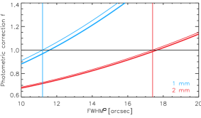
Figure 20: Magnitude of the beam photometric correction $f(\sigma)$ as a function of the actual FWHM, at 1 mm (blue) and 2 mm (red). Thick lines correspond to a choice of $\sigma_{\star}$ derived on a very bright source like Uranus. Thin lines are for sources of 1 Jy at 1 and 2 mm.

The beam size in stable atmospheric conditions $\sigma_{\star}$ is determined by fitting the 2D Gaussian beam on the series of scans of source with varying flux densities that have been used for the beam characterization in Sect. 6.2. However, $\sigma_{\star}$ is not equivalent to the main beam Gaussian size since the side lobes and first error beams are not taken into account for this beam size monitoring. The $\sigma_{\star}$ estimates are slightly larger for bright sources due to the contribution of the first side lobes and error beams, which are above the noise level, in the Gaussian fit.

C.2 Monitoring of the temperature-induced beam size variation

The photometric correction thus relies on the measure of the current beam size $\sigma$. The induced uncertainties on the flux density measurements depend on the precision of the beam size determination. Here we consider two methods to monitor the beam size.

The temperature-induced beam size variation is primarily monitored using 2D Gaussian fit on all the available bright source observations, as presented in Sect. 8.3.

For a finer sampling of the observation time, we also consider using the pointing scans for beam monitoring. As discussed in Sect. 3.2, the telescope pointing is monitored on a hourly basis during observation using pointing scans. As these scans consist of two sub-scans in azimuth and elevation of about 10 seconds of integration time each, they can also be used to make a map of the pointing source. For each campaign, we thus have on hands hundreds of maps of mostly point-like bright sources, which can also be used to monitor the beam size. For this purpose, pointing scans are reduced and projected onto maps of $2^{\prime\prime}$ resolution using the data analysis pipeline described in Sect. 4. Fitting an elliptical 2D Gaussian to this map, we compute the geometrical FWHM.Pointing scans on slightly extended sources, such as NGC7027, are discarded from the analysis.

For each pointing, we also seek for signs of atmospheric anomalous refraction. There are enough KIDs per observation band to make an independent map using only one subscan, i.e. 10 seconds of integration time. For each of the four cross subscans, we thus estimate the position of the best 2D Gaussian that fits the map. We compute the deviation between each subscan-derived position and the best-fit position using the entire scan. An anomalous refraction event is detected when the difference is above $2.5^{\prime\prime}$ for at least one subscan. We find that the temperature-induced beam size variation effect is due to anomalous refraction for between one third and one half of the scans, as reported in Sect. 8.3.

The pointing-based FWHM estimates constitute a time-sampling of the beam size during the whole observation campaign. They can serve to estimate the beam size of any observation scans, in particular towards sources too faint for a direct FWHM fit to be made on the map. However, we expect less accuracy than using standard OTF raster scans of bright sources due to the shorter integration time and the fact that only the innermost KIDs in the array see the source. To mitigate the dispersion, the time-stamped pointing-based FWHM is filtered with a running median on a 70-minute width time window. Then, the FWHM at the time of the considered scans is interpolated from the median-filtered pointing-based FWHM.

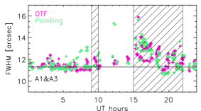
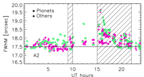
Figure 21: Beam size monitoring. ’OTF’-labelled pink data points show the FWHM estimates from a 2D Gaussian fit on the maps of OTF raster scans towards bright sources, whereas the ’Pointing’-labelled light green data points are FWHM estimates obtained by interpolating the median-filtered pointing-based FWHM at the time of the scans. The pointing-based FWHM estimates are obtained by fitting a 2D Gaussian on the maps of pointing scans.

Figure 21 shows two different FWHM estimates for the same data set: on one hand the best-fit FWHM estimates on the OTF-scan map and on the other hand the interpolation from the pointing-based FWHM monitoring. The two estimates show the same global variations as a function of the UT hours. They are well in agreement with each other, although the pointing-based estimates have more dispersion and a few outliers as expected.

C.3 The two case studies

We perform two case studies that correspond to the two beam monitoring methods discussed above.

Demonstration case This method named PC-demo hereafter, uses a photometric correction based on the beam monitoring with bright source scans. Both the 2D Gaussian FWHM fit and the FWHM₀ photometry are performed on the map of the source. This method thus applies only to point-like sources that are bright enough for an accurate fit of the beam on a single scan.

To capture only the beam size variations driven by the observing conditions (primary mirror deformations, anomalous refraction, elevation), a small correction $\delta_{\rm{FWHM}}$ has to be made to the 2D Gaussian beam FWHM estimate for bright sources. The estimate of the actual Gaussian size $\sigma$ is

$$\hat{\sigma}=\frac{(\rm{FWHM}-\delta_{\rm{FWHM}})}{2\sqrt{2\ln{2}}},$$ (38)

where the offset $\delta_{\rm{FWHM}}$ is null for faint or moderately bright point sources, and non-zero for bright sources. As for $\sigma_{\star}$, the 2D Gaussian fit yields slightly broader FWHM for bright sources (e.g. planets) to accommodate for the side lobes and error beams that are measured with high signal-to-noise. For Uranus, $\delta_{\rm{FWHM}}$ includes also the beam widening due to Uranus disc, as discussed in Sect. 6.2.3. We measure Uranus $\delta_{\rm{FWHM}}$ by comparing the average FWHM estimates using Uranus scans and using MWC349 scans, we found $\delta_{\rm{FWHM}}=0.4^{\prime\prime}$ at 1 mm and $\delta_{\rm{FWHM}}=0.25^{\prime\prime}$ at 2 mm, which basically distributes as one half being due to Uranus finite extension and the other half stemming from the side lobes.

Practical case using pointing scans This method, named PC-point hereafter, performs a photometric correction based on the beam monitoring with pointing scans. Unlike PC-demo, this method is usable even for sources fainter than about one Jy but relies on interpolations between beam width estimates on other scans. For Uranus, this value is corrected for the diameter size, as in Sect. 6.2.3. No other FWHM offset correction is needed since pointing scan maps have a low signal-to-noise ratio that prevents the geometrical FWHM from being significantly affected by the side lobes.

C.4 Absolute calibration with a photometric correction

We perform the absolute calibration by i) implementing the reference method described in Sect. 8.1.4, ii) correcting the atmospheric attenuation using the corrected skydip opacity estimates, and iii) using the photometric correction of Appendix C.1.

\begin{overpic}[clip={true},trim=0.0pt -8.5359pt -8.5359pt 0.0pt,width=227.64784pt]{Figures/plot_flux_density_ratio_fwhm_uranus_corrected_skydip_photocorr_demo_narrow_1mm.pdf} \put(18.0,25.0){\footnotesize PC-demo} \end{overpic}

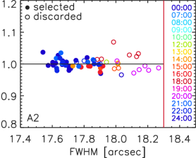
\begin{overpic}[clip={true},trim=0.0pt -8.5359pt -8.5359pt 0.0pt,width=227.64784pt]{Figures/plot_flux_density_ratio_fwhm_uranus_corrected_skydip_photocorr_pointing_narrow_1mm.pdf} \put(18.0,25.0){\footnotesize PC-point} \end{overpic}

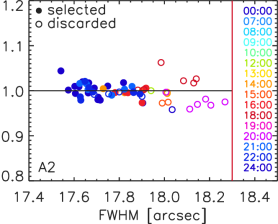
Figure 22: Uranus flux density ratio vs beam size for calibration with photometric correction. The ratio of Uranus measured flux densities to expectations as a function of the measured 2D Gaussian beam FWHM is shown for the $1$-mm array combination (left column) and for array 2 (right column) after absolute calibration using (first row) the PC-demo and (second row) the PC-point photometric corrections. These plots include all Uranus scans acquired during N2R9, N2R12 and N2R14 campaigns and whose beam FWHMs are below the threshold indicated by the vertical red lines, (open circles), as well as the scans that met the baseline scan selection criteria (filled circles). 38 scans now pass the baseline selection criteria vs 26 only without photometric correction (see also Fig. 13).

Using the photometric correction alleviates the need of performing a scan selection based on the observation time. However, the scans from which the absolute calibration is derived, are selected on the FWHM estimate using the same criteria as for the baseline calibration, that are FWHM thresholds of $12.5^{\prime\prime}$ at $1\,\rm{mm}$ and $18^{\prime\prime}$ at $2\,\rm{mm}$. Thus, only the scans that are moderately affected by the beam effect are included in the absolute calibration in order not to include twice the photometric correction uncertainties in the error budget (once for the absolute calibration and once for the photometry).

Figure 22 presents the Uranus measured-to-predicted flux density ratio as a function of the beam FWHM after the photometric correction with the PC-demo and PC-point methods. The flux density is stable against the beam FWHM within uncertainties for both wavelengths.

Table 21: Comparison of absolute calibration results using five methods

		baseline	TM	SD	PC-d	PC-p
$\#$ scans		26	26	26	38	38
Ratio	1mm	1.00	0.95	1.06	1.01	1.01
	2mm	1.00	0.94	0.99	1.01	1.01
RMS	1mm	3.3	4.5	3.3	3.1	2.6
$[\%]$	2mm	1.6	2.6	1.5	1.5	1.5

We further quantify the difference between all the calibration methods that have been tested in evaluating i) the average absolute calibration factor with respect to the baseline calibration factor and ii) the rms dispersion of the measured-to-modelled flux ratios. These quantities are gathered in Table 21 in the rows labelled ’Ratio’ and ’RMS’ respectively.

We find that, resorting to a photometric correction i) allows us to use $45\%$ more scans for the absolute calibration, ii) has a negligible impact on the absolute calibration factor and iii) yields a small reduction of the flux density ratio dispersion. For the absolute calibration, the PC-point method performs as well as the PC-demo one. Photometry capability and stability when using a photometric correction are further tested in Sect. 9.