Schwarz iteration method for elliptic equation with rough media based on random sampling

Abstract

We propose a computationally efficient Schwarz method for elliptic equations with rough media. A random sampling strategy is used to find low-rank approximations of all local solution maps in the offline stage; these maps are used to perform fast Schwarz iterations in the online stage. Numerical examples demonstrate accuracy and robustness of our approach.

65N30, 65N55

1 Introduction

Many problems of fundamental importance in science and engineering have structures that span several spatial scales. To give two examples, airplane wings constructed from fiber-reinforced composite materials and the permeability of groundwater flows modeled by porous media can both be described by partial differential equations (PDEs) whose coefficients have multiscale structure. Direct numerical simulation for these problems is difficult because the discretized system has very many degrees of freedom. Domain decomposition and parallel computing are usually needed to solve the discretized system.

Different types of PDEs typically require different strategies to overcome the computational difficulties arising from multiple scales. Computations with elliptic PDEs on rough media are termed “numerical homogenization,” for which several approaches have been proposed. The most well-known algorithms include the Generalized Finite Element Method (GFEM)[5, 4], Heterogeneous Multiscale Methods (HMM) [2, 9], Multiscale Finite Element Methods (MsFEM) [11, 16], local orthogonal decomposition [17], and local basis construction [21, 20]. Most of these methods divide the computation into offline and online stages. The offline step finds local bases that are adaptive to local properties and capture small-scale effects on the macroscopic solutions. In the online step, a global stiffness matrix is assembled in such a way that this small-scale information is implanted and preserved. The online computation is performed on a coarse grid, thus reducing computational costs. Alternative approaches use a domain decomposition framdwork to target directly the problem on the fine mesh (see, for example, [14, 18, 23, 8, 22] and references therein). These methods are typically iterative, dividing the domain into patches to allow for parallel computation. The most important issues for these approaches are (1) the local solvers need to resolve the fine grids, which drives up computational costs; and (2) the convergence rate depends on the conditioning, so many iterations are required for an ill-conditioned problem. Several strategies have been proposed to overcome these issues. One such strategy is to use MsFEM as a preconditioner for the Schwarz method [1] or to construct coarse spaces via solution of local eigenvalue problems [12, 10]. This preconditioner differs from the traditional domain decomposition preconditioner in that the coarse solver is adaptive to the small scale features. In contrast to the deterioration of traditional preconditioner when multiscale structure is present, its adaptive counterpart is nearly independent of high contrast and of small scales within the media [1, 13].

We propose a rather different perspective for numerical homogenization, under the framework of domain decomposition with Schwarz iteration. The homogenization phenomenon for elliptic equations with highly oscillatory media refers to the fact that its solution can be approximated by the solution to an effective equation that has no oscillation in the media [3]. Although it is not always easy to identify the effective equation explicitly, just the knowledge that it exists allows us to argue that the equation can be “compressed” in some sense. One still needs to understand what aspect, exactly, can be “compressed.” In our previous work [6], we demonstrated that the collection of Green’s functions, when discretized and stored in a matrix form, can be compressed approximately into a low-dimensional space spanned by its leading singular vectors. To obtain these representative basis functions, we apply a random sampling technique analogous to the one used in compressed sensing. In effect, we explored the counterpart of the randomized SVD (RSVD) algorithm [15] in the PDE setting, and in the framework of GFEM, we were able to capture the representative local $a$-harmonic functions at significantly reduced computational cost.

In this article, we argue there is another quantity that can be “compressed,” giving another route to higher numerical efficiency. In the Schwarz procedure, the whole domain is decomposed into multiple subdomains with small overlaps. At each iteration, a local solution is obtained on each patch, using boundary conditions for that patch supplied by its neighbors. These local solutions yield boundary conditions for neighboring patches, which are then used in the next round of Schwarz iteration. In effect, each local solution procedure is a boundary-to-boundary map. Each Schwarz iteration is contractive, so the overall procedure converges. The total cost is determined by the cost of local solvers, the number of subdomains, and the number of Schwarz iterations. The latter two can be balanced by using preconditioning techniques. The cost of the first factor — the boundary-to-boundary map — can be reduced by noting that this map is compressive. Its spectrum decays exponentially, so a compact approximation to this map can be obtained and applied rapidly, with accuracy sufficient to allow convergence of the outer Schwarz procedure. Only a few samples (in the form of randomized boundary conditions) are needed to approximate the boundary-to-boundary maps. These are performed in the offline stage. Our procedure can be regarded as a counterpart of an RSVD algorithm for a PDE solution operator. (Our approach in [6] approximates the range of the solution space instead.) This procedure was discussed in [7] for the case of the radiative transfer equation, where there are two scales both needing to be resolved. In this article, we target an elliptic homogenization problem. Our main contribution lies in bringing randomized sampling technique and incorporating it with multiscale domain decomposition methods. Our solver is adaptive to small scale features, inexpensive to build offline, and has fast online convergence.

In the remainder of the paper, we introduce fundamental concepts in Section 2 and describe our algorithm in Section 3, first reviewing RSVD and interpreting it in our setting. Computational results are shown in Section 4.

2 Schwarz method for elliptic equation

We review briefly the elliptic equation with rough media and its homogenization limit, then present an overview of Schwarz iteration method under the domain decomposition framework.

2.1 Elliptic equation with rough media

We consider the boundary value problem for a scalar second order elliptic equation with rough media:

(1) $$\begin{cases}\nabla\cdot(a^{\varepsilon}(x)\nabla u^{\varepsilon}(x))=0\,,&\mbox{\rm in $\Omega\subset\mathbb{R}^{d}$}\\ u^{\varepsilon}(x)=b(x)\,,&\mbox{\rm on $\partial\Omega$,}\end{cases}$$

where the function $a^{\varepsilon}(x)\in L^{\infty}(\Omega)$ models the media. This is the typical governing equation in the modeling of water flow in porous media and heat diffusion through composite materials. In these examples, the media tensor $a^{\varepsilon}(x)$ usually exhibits multiscale structure; the parameter $\varepsilon$ denotes the smallest scale that appears explicitly in the media. The media $a^{\varepsilon}(x)$ is assumed to be uniformly bounded, namely $\alpha\leq a^{\varepsilon}(x)\leq\beta$. The Dirichlet boundary condition $f(x)$ is a macroscopic quantity that usually does not contain small scales, that is, it is independent of $\varepsilon$. For simplicity, we restrict ourselves to the case in which $d=2$.

For equations demonstrating certain structures, the asymptotic limit of the equation can be derived. In particular, when the media is pseudo-periodic, this homogenization procedure is classical. Denoting

$$a^{\varepsilon}(x)=a(x,{x}/{\varepsilon})=a(x,y)\,,\quad\text{with}\quad y={x}/{\varepsilon}$$

and assuming that $a(x,y)$ is periodic in the fast variable $y$, we have the following theorem:

Theorem 2.1.

([19, Theorem 2.1]]) Assuming a priori that $u^{\ast}\in H^{2}(\Omega)$, then there exists constant $C>0$ such that

$$\|u^{\varepsilon}-u^{\ast}\|_{L^{2}(\Omega)}\leq C\varepsilon\|u^{\ast}\|_{H^{2}(\Omega)}$$

where $u^{\varepsilon}$ is the solution to equation (1) and $u^{\ast}$ the solution to the following effective equation

(2) $$\begin{cases}\nabla\cdot(a^{\ast}(x)\nabla u^{\ast}(x))=0\,,&\mbox{\rm in $\Omega\subset\mathbb{R}^{d}$}\\ u^{\ast}(x)=b(x)\,,&\mbox{\rm on $\partial\Omega$.}\end{cases}$$

Although it is not easy to find the smooth effective media $a^{\ast}$ except in some very special cases, the theorem suggests that the asymptotic limit of the equation with highly oscillatory media is one that has smooth media. This observation, when interpreted correctly, can lead to significant improvements in computation. A naive discretization method applied to (1) would require discretization with $\Delta x\ll\varepsilon$, while in the limit, assuming $a^{\ast}$ is known, the problem (2) could be solved with discretization $\Delta x=o(1)$, leading to a much less expensive computation.

Our approach exploits this observation. In Section 3, we demonstrate that the boundary-to-boundary map used in Schwarz iteration is indeed compressible, and a random sampling technique can be used to approximate this map cheaply, leading to computational savings. Importantly, though, our approach does not require explicit knowledge of the limiting medium $a^{\ast}$.

2.2 Domain decomposition and Schwarz iteration

The Schwarz iteration procedure based on domain decomposition divides the physical domain $\Omega$ into many overlapping subdomains, obtains local solutions on the subdomains, exchanges information in the form of boundary conditions for the subdomains, and repeats the whole procedure until convergence. We denote by $\{\Omega_{i}\,,i=1,\ldots,N\}$ an open cover of $\Omega$ (see Fig. 1), so that

(3) $$\Omega=\cup_{i=1}^{N}\Omega_{i}\,.$$

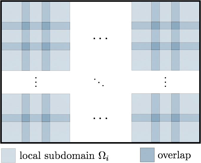
Figure 1: An overlapping domain decomposition of rectangular domain $\Omega$ in 2D

Defining the collection of indices of the subdomains that intersect with $\Omega_{i}$ as follows:

(4) $$\mathcal{I}_{i}=\{j\in\mathbb{Z}:\Omega_{i}\cap\Omega_{j}\neq\emptyset\}\,,$$

the interior of each subdomain $\Omega_{i}$ can be written as follows:

(5) $$\widetilde{\Omega}_{i}=\Omega_{i}\cap\left(\cup_{j\in\mathcal{I}_{i}}\Omega_{j}^{c}\right)\,,$$

where $\Omega_{j}^{c}$ denotes the complement of $\Omega_{j}$. The global solution $u^{\varepsilon}$ to (1) can be expressed as a superposition of many modified local solutions:

(6) $$u^{\varepsilon}(x)=\sum_{i=1}^{N}\eta_{i}(x)u^{\varepsilon}_{i}(x)\,,$$

where $u^{\varepsilon}_{i}(x)$ is the local solution on $\Omega_{i}$, satisfying the same elliptic equation locally over the subdomain $\Omega_{i}$:

(7) $$\begin{cases}\nabla\cdot(a^{\varepsilon}(x)\nabla u_{i}^{\varepsilon}(x))=0\,,&\mbox{\rm in $\Omega_{i}$}\\ u_{i}^{\varepsilon}(x)=f_{i}(x)\,,&\mbox{\rm on $\partial\Omega_{i}$,}\end{cases}$$

and $\eta_{i}(x)$, $i=1,2,\dotsc,N$ are the partition-of-unity functions satisfying

$$\sum_{i=1}^{N}\eta_{i}(x)=1\,,\quad\forall x\in\Omega\,,\quad\text{with}\quad\begin{cases}0\leq\eta_{i}(x)\leq 1\,,&x\in\Omega_{i}\\ \eta_{i}(x)=0\,,&x\in\Omega\backslash\Omega_{i}.\end{cases}$$

The collection of local boundary conditions $f=[f_{1}(x)\,,\dotsc f_{N}(x)]$ are the unknowns in the iteration, found by updating solutions in local patches iteratively until adjacent patches coincide in the regions of overlap. Upon finding $f$, one finds the entire global solution using (6).

The Schwarz method starts by assigning initial guesses to the local boundary conditions $f_{i}(x)$, then solves all subproblems (7), possibly in parallel. The local solutions $u_{i}^{\varepsilon}(x)$ so obtained are then used to update local boundary conditions for those neighboring subdomains whose boundaries are contained in $\Omega_{i}$ (that is, the subdomains denoted by $\mathcal{I}_{i}$ in (4)). The procedure can be summarized as follows:

(8) $$f_{i}(x)\xrightarrow{\mathcal{S}_{i}}u_{i}(x)\xrightarrow{\mathcal{P}_{i}}f_{j}(x)\,,\text{ for all }j\in\mathcal{I}_{i},$$

where $\mathcal{S}_{i}$ the solution operator of equation (7) over subdomain $\Omega_{i}$ and $\mathcal{P}_{i}$ is the restriction operator of the solution to the neighboring boundaries $\partial\Omega_{j}$ ($j\in\mathcal{I}_{i}$). Defining the boundary-to-boundary map by $\mathcal{A}_{i}:=\mathcal{P}_{i}\circ\mathcal{S}_{i}$, and defining $\mathcal{A}$ to be the aggregation of $\mathcal{A}_{i}$ over $i=1,2,\dotsc,N$, one can denote

$$f^{\text{new}}=\mathcal{A}f^{\text{old}}\,.$$

The overall procedure is summarized in Algorithm 1. The total CPU time for this method is approximately the product of the number of iterations $T$ and the CPU time $\tau$ for each iteration. While $T$ depends on the conditioning of the system, the value of $\tau$ is determined by the cost of solving the local equation (7).

Algorithm 1 Schwarz method for equation (1)

1:  Given total iterations $T$, boundary condition $f$;

2:  For $i=1,2,\dotsc,N$, initiate $f_{i}^{0}(x)=b(x)$ for $x\in\partial\Omega\cap\partial\Omega_{i}$ and assign $f_{i}^{0}(x)=0$ elsewhere;

3:  $t\leftarrow 0$;

4:  while $t<T$ do

5:     for $i=1,\ldots,N$ do

6:        Load $f_{i}^{t}$ as boundary condition for equation (7) and solve for $u_{i}^{t}(x)$;

7:        Update $f_{j}^{t+1}(x)=u_{i}^{t}(x)\,,x\in\Omega\cap\partial\Omega_{j}$ for all $j\in\mathcal{I}_{i}$;

8:     end for

9:  end while

10:  For $i=1,2,\dotsc,N$, load $f_{i}^{T}$ as boundary condition for equation (7) and solve for $u^{T}_{i}(x)$;

11:  Assemble global solution $u^{T}(x)=\sum_{i=1}^{N}\eta_{i}(x)u^{T}_{i}(x)$;

12:  return  $u^{T}(x)$.

3 Schwarz method based on random sampling

In this section, we propose a new algorithm that incorporates random sampling into Schwarz iteration, under the domain decomposition framework. As discussed above, each iteration requires the solution of many subproblems, so the cost of obtaining local solutions is critical to the overall run time. The key operation is the boundary-to-boundary map $f^{t+1}=\mathcal{A}f^{t}$, which maps the boundary conditions for the patches at iteration $t$ of the Schwarz procedure to an updated set of boundary conditions obtained by solving the subproblems on the patches, then restricting the solution to the patch boundaries. This map can be prepared offline. Moreover, by noting that the equation is “homogenizable” to an effective equation, we show that the boundary-to-boundary map has approximately low rank. Techniques inspired by from randomized linear algebra can be used to find the low-rank approximation efficiently.

Our main tool is the randomized SVD algorithm. It is was shown in [15] that by multiplying a low-rank matrix and its transpose by several i.i.d. Gaussian vectors, and performing several other inexpensive operations, the rank information could be captured with high accuracy and high probability. We translate this technique to the PDE setting and use it to reduce the cost of the boundary-to-boundary map.

Since the random sampling technique plays a crucial role in finding the approximated map, we quickly review the randomized SVD algorithm of [15] in Section 3.1. This algorithm requires a matrix-vector operation involving the adjoint matrix, and in the PDE setting, we need to find the adjoint associated with the boundary-to-boundary map, an operation discussed in in Section 3.2. At the end of this section, we integrate all components and summarize the algorithm.

3.1 Random sampling for low rank matrices

Random sampling algorithms have been widely used in numerical linear algebra and machine learning. They are powerful in extracting efficiently the main features of objects whose intrinsic dimension is much smaller than their apparent dimension, such as sparse vectors, low-rank matrices, or low-dimensional manifolds. We review the randomized SVD algorithm applied on a large matrix $\mathsf{A}\in\mathbb{R}^{m\times n}$ with $m\geq n$. The SVD of $\mathsf{A}$ is

$$\mathsf{A}=\mathsf{U}\Sigma\mathsf{V}^{\top}=\sum_{i=1}^{n}\sigma_{i}u_{i}v_{i}^{\top}\,,$$

where $\mathsf{U}=[u_{1},\ldots,u_{n}]\in\mathbb{R}^{m\times n}$ contains the left singular vectors, $\mathsf{V}=[v_{1},\ldots,v_{n}]$ contains the right singular vectors and $\Sigma=\text{diag}(\sigma_{1},\ldots,\sigma_{n})$ contains the singular values in decreasing order: $\sigma_{1}\geq\sigma_{2}\geq\ldots\sigma_{n}\geq 0$. If $\mathsf{A}$ has approximate rank $k$, the best rank-$k$ approximation of $\mathsf{A}$ is the truncated rank-$k$ singular value decomposition

$$\mathsf{A}_{k}:=\mathsf{U}_{k}\Sigma_{k}\mathsf{V}^{\top}_{k}=\sum_{i=1}^{k}\sigma_{i}u_{i}v_{i}^{\top}\,,$$

where $\mathsf{U}_{k}$ and $\mathsf{V}_{k}$ collect the first $k$ columns of $\mathsf{U}$ and $\mathsf{V}$, respectively, and $\Sigma_{k}$ is the principal $k\times k$ major of $\Sigma$. The relative error of this approximation is given by

$$\frac{\|\mathsf{A}-\mathsf{A}_{k}\|_{2}}{\|\mathsf{A}\|_{2}}=\frac{\sigma_{k+1}}{\sigma_{1}}\ll 1\,.$$

Computation of the singular value decomposition of $\mathsf{A}$ requires $\mathcal{O}(mn^{2})$ time, which is expensive for large $m$ and $n$. The randomized SVD algorithm computes an approximation to $\mathsf{A}_{k}$ by simply applying the matrix $\mathsf{A}$ to a relatively few random i.i.d. Gaussian vectors. The prototype randomized SVD algorithm is shows as Algorithm 2.

Algorithm 2 Randomized SVD algorithm

1:  Given an $m\times n$ matrix $\mathsf{A}$, target rank $k$;

2:  Stage A:

3:  Generate an $n\times 2k$ Gaussian test matrix $\Omega$;

4:  Form $\mathsf{Y}=\mathsf{A}\Omega$;

5:  Perform the QR-decomposition of $\mathsf{Y}$: $\mathsf{Y}=\mathsf{Q}\mathsf{R}$

6:  Stage B:

7:  Form $\mathsf{B}=\mathsf{A}^{\top}\mathsf{Q}$;

8:  Compute the SVD of the $2k\times n$ matrix $\mathsf{B}^{\top}=\widetilde{\mathsf{U}}\Sigma\mathsf{V}^{\top}$;

9:  Set $\mathsf{U}=\mathsf{Q}\widetilde{\mathsf{U}}$;

10:  return  $\mathsf{U},\Sigma,\mathsf{V}$.

For completeness, we give the error estimate result.

Theorem 3.1.

([15, Theorem 10.8])  Algorithm 2 finds accurate SVD of $\mathsf{A}$ in expectation:

$$\mathbb{E}\|\mathsf{A}-\mathsf{U}\Sigma\mathsf{V}^{\ast}\|\leq\left[1+4\sqrt{\frac{2\min\{m,n\}}{k-1}}\right]\sigma_{k+1}\,,$$

Algorithm 2 requires time complexity

(9) $$T_{\text{randSVD}}=2kT_{\text{mult}}+\mathcal{O}(k^{2}(m+n))\,,$$

where $2kT_{\text{mult}}$ is the time complexity of matrix-vector multiplication with $\mathsf{A}$ and $\mathsf{A}^{\top}$. We note that assuming $\mathsf{A}$ is approximately of low rank $k\ll\min\{m,n\}$, the complexity is rather low, and with fast decaying $\sigma_{k}$, the error is small too.

3.2 Adjoint map

We aim at integrating the randomized SVD algorithm into the framework of Schwarz method. As described in Algorithm 1, each time step amounts to an update of the boundary conditions $f$ on the patches, and has the form

(10) $$f^{t+1}=\mathcal{A}f^{t}(x)\,,\quad\text{with}\quad\mathcal{A}_{i}=\mathcal{P}_{i}\circ\mathcal{S}_{i}\,.$$

where $\mathcal{S}_{i}$ is a solution operator and $\mathcal{P}_{i}$ is a restriction operator, both discussed further below. Since the equation is homogenizable, many degrees of freedom can be neglected, making $\mathcal{A}_{i}$ approximately low rank. Algorithm 2 is therefore relevant, but there is an immediate difficulty. After applying the full matrix (or operator) to some random vectors in Stage A, we need in Stage B to apply the transpose or adjoint to given vectors $q_{i}$. For the operator define in (10), we need to know how to operate with both $\mathcal{A}_{i}\xi$ and $\mathcal{A}^{\ast}_{i}\zeta$ for any given $\xi$ and $\zeta$. Computing $\mathcal{A}_{i}\xi$ is rather straightforward: it amounts to set local boundary condition being $\xi$ and find the solution’s confinement on the neighboring cells’ boundaries. Operating with the adjoint $\mathcal{A}_{i}^{\ast}$ is somewhat more complicated.

A second difficulty has to do with the nature of the low rank of $\mathcal{A}_{i}$. In general, the solution map $\mathcal{S}_{i}$ does not have low rank, as we see in Section 4. We can however identify a confined solution map $\widetilde{\mathcal{S}}_{i}$, which maps the boundary condition on $\partial\Omega_{i}$ to the interior solution $\widetilde{\Omega}_{i}$. By composing with the restriction operator $\mathcal{P}_{i}$ (slightly redefined), we obtain the same $\mathcal{A}_{i}$ of (10). It happens that this confined operator $\widetilde{\mathcal{S}}_{i}$ has approximately low rank.

Specifically, we define $\widetilde{\mathcal{S}}_{i}$ as follows: Given the boundary condition $f$ over $\partial\Omega_{i}$, we have $\widetilde{\mathcal{S}}_{i}f=u|_{\widetilde{\Omega}_{i}}$, where $u$ solves the system

$$\nabla\cdot(a^{\varepsilon}(x)\nabla u(x))=0\,,\text{ in }\Omega_{i}\quad\text{with}\quad u(x)=f(x)\,,\text{ on }\partial\Omega_{i}\,.$$

We then rewrite (10) as follows:

(11) $$f^{t+1}=\mathcal{A}f^{t}(x)\,,\quad\text{with}\quad\mathcal{A}_{i}=\mathcal{P}_{i}\circ\widetilde{\mathcal{S}}_{i}\,.$$

To find the adjoint of $\widetilde{\mathcal{S}}_{i}$ we show the following theorem.

Theorem 3.2.

Given two open sets $\widetilde{\Omega}$ and $\Omega$ such that $\overline{\widetilde{\Omega}}\subset\Omega$, then for arbitrary $f\in H^{1/2}(\partial\Omega)$ and $g\in H^{1}(\widetilde{\Omega})$, we have

(12) $$\langle g,\widetilde{\mathcal{S}}f\rangle_{\widetilde{\Omega}}=\langle\widetilde{\mathcal{S}}^{\ast}g,f\rangle_{\partial\Omega},$$

where $\widetilde{\mathcal{S}}$ and $\widetilde{\mathcal{S}}^{\ast}$ are defined as follows:

(13) $$\widetilde{\mathcal{S}}: \quad H^{1/2}(\partial\Omega) \rightarrow \quad H^{1}(\widetilde{\Omega})$$

$$\quad f \mapsto \quad u|_{\widetilde{\Omega}},$$

where $u$ is the solution of the following elliptic equation:

(14) $$\begin{cases}\nabla\cdot(a(x)\nabla u(x))=0\,,&\mbox{\rm in $\Omega$}\\ u(x)=f(x)\,,&\mbox{\rm on $\partial\Omega$},\end{cases}$$

and

(15) $$\widetilde{\mathcal{S}}^{\ast}: \quad H^{1}(\widetilde{\Omega}) \rightarrow \quad H^{-1/2}(\partial\Omega)$$

$$\quad g \mapsto \quad a\frac{\partial v}{\partial n},$$

where $v$ solves the following sourced elliptic equation:

(16) $$\begin{cases}\nabla\cdot(a(x)\nabla v(x))=\widetilde{g}\,,&\mbox{\rm in $\Omega$}\\ v(x)=0(x)\,,&\mbox{\rm on $\partial\Omega$,}\end{cases}$$

and $\widetilde{g}$ is the zero extension of $g(x)$ over $\Omega$.

Proof 3.3.

Notice that the term on the left in Eq. 12 is

(17) $$\langle g,\widetilde{\mathcal{S}}f\rangle_{\widetilde{\Omega}}=\int_{\widetilde{\Omega}}gu=\int_{\Omega}\widetilde{g}u=\int_{\Omega}u\nabla\cdot(a\nabla v).$$

Here $\langle\cdot,\cdot\rangle_{\widetilde{\Omega}}$ denotes the $L^{2}$ pairing over $\widetilde{\Omega}$ and the second and third equality comes from the definition of $\widetilde{g}$. Applying Green’s second identity, we obtain

(18) $$\int_{\Omega}\left[u\nabla\cdot(a\nabla v)-v\nabla\cdot(a\nabla u)\right]=\int_{\partial\Omega}a\left(u\frac{\partial v}{\partial n}-v\frac{\partial u}{\partial n}\right).$$

By comparing (17) and (18), we have

$$\langle g,\widetilde{\mathcal{S}}f\rangle_{\widetilde{\Omega}} =\int_{\Omega}v\nabla\cdot(a\nabla u)+\int_{\partial\Omega}a\left(u\frac{\partial v}{\partial n}-v\frac{\partial u}{\partial n}\right)$$

$$=\int_{\partial\Omega}u\left(a\frac{\partial v}{\partial n}\right)$$

$$=\int_{\partial\Omega}f\left(a\frac{\partial v}{\partial n}\right)$$

$$=\langle\widetilde{\mathcal{S}}^{\ast}g,f\rangle_{\partial\Omega},$$

where we use (14) and (16). Thus (12) is proved.

This theorem shows how to evaluate the adjoint operator $\widetilde{\mathcal{S}}^{\ast}_{i}$, thus making it possible to adapt the randomized SVD approach of Algorithm 2 to our setting. We summarize the resulting method as Algorithm 3. It requires only $k$ solves of local elliptic PDE (7) and sourced elliptic PDE (16), together with a QR factorization and SVD of relatively small matrices.

Algorithm 3 Randomized SVD for $\widetilde{\mathcal{S}}_{i}$

1:  Given target rank $k$ (an even number) and numerical solver for (7) and (16);

2:  for $j=1,\ldots,k$ do

3:     Generate random boundary conditions $\xi_{j}$ over $\partial\Omega_{i}$;

4:     Load $\xi_{j}$ as boundary condition in (7), and solve to obtain $u_{j}$;

5:     Take restrictions of $u_{j}$ over $\widetilde{\Omega}_{i}$ to obtain $\widetilde{u}_{j}$;

6:  end for

7:  Find orthonormal basis $Q=[q_{1},\ldots,q_{k}]$ of $\widetilde{U}:=\{\widetilde{u}_{1},\ldots,\widetilde{u}_{k}\}$;

8:  for $j=1,\ldots,k$ do

9:     Construct zero extension of $q_{k}$ over $\Omega_{i}$, denoted by $\widetilde{q}_{k}$;

10:     Load $\widetilde{q}_{k}$ as source in (16), and solve to obtain $v_{j}$;

11:     Compute boundary flux $b_{j}:=a\frac{\partial v_{j}}{\partial n}$;

12:  end for

13:  Assemble all fluxes $B=[b_{1},\ldots,b_{k}]$;

14:  Compute SVD of $B^{\ast}=\widetilde{\mathsf{U}}_{k}\Sigma_{k}\mathsf{V}_{k}^{\ast}$;

15:  Compute $\mathsf{U}_{k}=Q\widetilde{\mathsf{U}}_{k}$;

16:  return  $\mathsf{U}_{k},\Sigma_{k},\mathsf{V}_{k}$.

This procedure can be executed offline to produce a rank-$k$ approximation to $\widetilde{\mathcal{S}}_{i}$. In online execution of the Schwarz iteration procedure, Algorithm 1, the update procedure (8) can be modified by replacing $\widetilde{\mathcal{S}}_{i}$ with its low rank approximation, defined as follows:

(19) $$f_{i}(x)\xrightarrow{\mathsf{U}_{k}\Sigma_{k}\mathsf{V}_{k}^{\ast}}\widetilde{u}^{t}_{i}(x)\xrightarrow{\mathcal{P}_{i}}f_{j}(x)\,,\text{ for all }j\in\mathcal{I}_{i}.$$

We summarize our reduced Schwarz procedure as Algorithm 4.

Algorithm 4 Reduced Schwarz method for (1)

1:  Given rank $k$, total iterations $T$, boundary condition $b$;

2:  Offline:

3:  for $n=1,\ldots,N$ do

4:     Use Algorithm 3 to find the rank-$k$ RSVD of $\widetilde{\mathcal{S}}_{i}$, denoted by $\mathsf{U}_{k}^{i}\Sigma_{k}^{i}\mathsf{V}_{k}^{i,\ast}$;

5:  end for

6:  Online:

7:  Initiate $f_{i}^{0}(x)=b(x)$ for $x\in\partial\Omega\cap\partial\Omega_{i}$ and assign $f_{i}^{0}(x)=0$ elsewhere;

8:  while $t<T$ do

9:     for $n=1,\ldots,N$ do

10:        Evaluate $\widetilde{u}_{i}^{t}=\mathsf{U}_{k}^{i}\Sigma_{k}^{i}\mathsf{V}_{k}^{i,\ast}f_{i}^{t}$;

11:        Update $f_{j}^{t+1}(x)=\widetilde{u}_{i}^{t}(x)\,,x\in\Omega\cap\partial\Omega_{j}$, for all $j\in\mathcal{I}_{i}$;

12:     end for

13:  end while

14:  for $n=1,\ldots,T$ do

15:     Load $f_{i}^{T}$ as boundary condition for equation (7) and solve for $u^{T}_{i}(x)$;

16:  end for

17:  Assemble global solution $u^{T}(x)=\sum_{n=1}^{N}\eta(x)u^{T}_{i}(x)$;

18:  return  $u^{T}(x)$;

4 Numerical Experiments

In this section, we report on several numerical tests that demonstrate effectiveness of our algorithm. We consider (1) with a highly oscillatory media $a^{\varepsilon}(x,y)$:

$$a^{\varepsilon}(x,y)=\frac{2+1.8\sin(\pi x/\varepsilon)}{2+1.8\cos(\pi y/\varepsilon)}+\frac{2+\sin(\pi y/\varepsilon)}{2+1.8\sin(\pi x)}\,,\quad(x,y)\in\Omega=[0,10]\times[0,1]\,,$$

with $\varepsilon={1}/{16}$. This media is plotted in Fig. 2.

Figure 2: Graph of highly oscillatory media $a^{\varepsilon}(x,y)$

To resolve the small scale, the fine discretization parameter is set to $h=1/40$ in both $x$ and $y$ direction. For ease of implementation, we decompose the domain into subdomains in just one dimension, as follows:

$$\Omega=\cup_{i=0}^{12}\Omega_{n}\,,\quad\text{with}\quad\Omega_{i}:=\left[\frac{3i}{4},1+\frac{3i}{4}\right]\times[0,1]\,.$$

Each subdomain $\Omega_{i}$ is thus a unit square with one quarter margin overlapped with its neighbors on both sides. For this case, we have that $\mathcal{I}_{i}=\{i-1,i+1\}$ for all inner patches; see Fig. 3. The boundary condition is

$$b(x,y)=\sin\left(\frac{\pi}{3}(x-1/3)\right)\sin\left(3\pi(y-1/4)\right)\,,\quad\text{with}\quad(x,y)\in\partial\Omega\,.$$

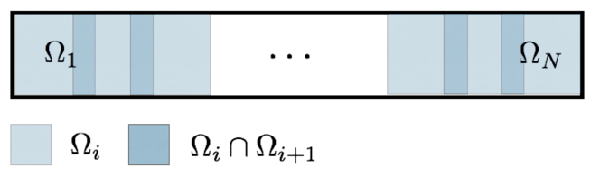
Figure 3: An overlapping domain decomposition of $\Omega$. Each subdomain $\Omega_{i}$ overlaps with its neighbors with one quarter margin.

In the next two subsections, we discuss the results of the offline operation (low-rank approximation of the boundary-to-boundary map) and the online iteration results, respectively.

4.1 Reducibility of update procedure

As described above, the mapping $\mathcal{A}_{i}$ is composed of a boundary-to-solution map composed with a trace-taking operation, defined by either (10) or (11). We claimed above that the the map $\widetilde{\mathcal{S}}_{i}$ is approximately low rank, while $\mathcal{S}_{i}$ is not. In Fig. 4, we plot the singular values of these two operators for subdomain $\Omega_{3}$, and observe these claims to hold for this subdomain. We also plot the singular values of $\mathcal{A}_{3}$, for which the low-rank structure is even more evident. Similar results hold for the other inner subdomains $\Omega_{i}$, $i=1,2,\dotsc,11$.

Figure 4: Singular values of operator $\mathcal{S}_{3},\widetilde{\mathcal{S}}_{3}$ and $\mathcal{A}_{3}$.

4.2 Performance of reduced Schwarz method

To demonstrate the accuracy and efficiency of our method, we run the reduced Schwarz method, Algorithm 4, for several values of the rank parameter ($k=40,70,100,130$) in each subdomain. The reference solution $u_{\text{ref}}$ is computed using the vanilla Schwarz method with $T=100$, at which iteration the relative difference between successive iterations reaches machine precision. In Fig. 5, we compare the reference solution to the solution produced by Algorithm 4 with $k=40$ and $T=50$. The difference is barely visible.

Figure 5: Left: Reference solution generated by running the Schwarz method with $100$ iterations; Right: Approximate solution generated by running the reduced Schwarz method with rank $k=40$ for $50$ iterations.

We document the relative errors defined by

$$\text{Relative Error}=\frac{\|u-u_{\text{ref}}\|_{2}}{\|u_{\text{ref}}\|_{2}}$$

at the iterates of both the vanilla Schwarz (Algorithm 1) and the reduced Schwarz (Algorithm 4) methods, the latter for various values of $k$. From this semilog plot, it is clear that error decays exponentially with iteration number in all cases, and at the same rate. Moreover, increasing $k$ allows the error to saturate at an increased level of accuracy. Still, with rank $k=70$ (just one third of the full basis), we are already able to capture an accuracy of $10^{-5}$.

Figure 6: Relative Error for Schwarz method and reduced Schwarz methods, for various ranks $k$. The relative error decreases exponentially in time, and saturates at different levels. A higher rank $k$ in the reduced Schwarz method causes the error to saturate at a higher level of accuracy.

To demonstrate efficiency, we report in Table 1 offline and online calculation time for reduced Schwarz method, and compare it with the vanilla Schwarz method. Although the reduced method is slower overall for solving a single instance, it is extremely fast in the online stage, implying that it is highly competitive if one needs to solve (1) for multiple different boundary conditions. (In this case, each new set of boundary conditions requires only the online stage to be performed in the reduced Schwarz procedure, whereas in vanilla Schwarz, the entire method needs to be executed again.)

Run Time (s)	Reduced Schwarz				Schwarz
	$k=40$	$k=70$	$k=100$	$k=130$
Offline Stage	49.7	87.3	129.4	167.4	0
Online Stage	.049	.061	.070	.068	31.4
Total Time	49.8	87.3	129.4	167.4	31.4

Table 1: Run times for the vanilla Schwarz method and the reduced Schwarz method for several values of $k$.

References

- [1] J. Aarnes and T. Y. Hou, Multiscale domain decomposition methods for elliptic problems with high aspect ratios, Acta Mathematicae Applicatae Sinica, 18 (2002), pp. 63–76.
- [2] A. Abdulle, E. Weinan, B. Engquist, and E. Vanden-Eijnden, The heterogeneous multiscale method, Acta Numerica, 21 (2012), pp. 1–87, https://doi.org/10.1017/S0962492912000025.
- [3] G. Allaire, Homogenization and two-scale convergence, SIAM Journal on Mathematical Analysis, 23 (1992), pp. 1482–1518, https://doi.org/10.1137/0523084.
- [4] I. Babuska and R. Lipton, Optimal local approximation spaces for generalized finite element methods with application to multiscale problems, Multiscale Modeling & Simulation, 9 (2011), pp. 373–406, https://doi.org/10.1137/100791051.
- [5] I. Babuška and J. Osborn, Generalized finite element methods: Their performance and their relation to mixed methods, SIAM Journal on Numerical Analysis, 20 (1983), pp. 510–536, https://doi.org/10.1137/0720034.
- [6] K. Chen, Q. Li, J. Lu, and S. J. Wright, Random sampling and efficient algorithms for multiscale PDEs, arXiv preprint arXiv:1807.08848, (2018).
- [7] K. Chen, Q. Li, J. Lu, and S. J. Wright, A low-rank Schwarz method for radiative transport equation with heterogeneous scattering coefficient, Technical Report arXiv:1906.02176, University of Wisconsin-Madison, June 2019.
- [8] V. Dolean, P. Jolivet, and F. Nataf, An introduction to domain decomposition methods: algorithms, theory, and parallel implementation, vol. 144, SIAM, 2015.
- [9] W. E and B. Engquist, The heterognous multiscale methods, Commun. Math. Sci., 1 (2003), pp. 87–132, https://projecteuclid.org:443/euclid.cms/1118150402.
- [10] Y. Efendiev, J. Galvis, and X.-H. Wu, Multiscale finite element methods for high-contrast problems using local spectral basis functions, Journal of Computational Physics, 230 (2011), pp. 937 – 955, https://doi.org/https://doi.org/10.1016/j.jcp.2010.09.026.
- [11] Y. Efendiev and T. Y. Hou, Multiscale finite element methods: theory and applications, vol. 4, Springer Science & Business Media, 2009.
- [12] J. Galvis and Y. Efendiev, Domain decomposition preconditioners for multiscale flows in high-contrast media, Multiscale Modeling & Simulation, 8 (2010), pp. 1461–1483, https://doi.org/10.1137/090751190.
- [13] J. Galvis and J. Wei, Ensemble level multiscale finite element and preconditioner for channelized systems and applications, Journal of Computational and Applied Mathematics, 255 (2014), pp. 456 – 467, https://doi.org/https://doi.org/10.1016/j.cam.2013.06.007, http://www.sciencedirect.com/science/article/pii/S0377042713003038.
- [14] I. G. Graham, P. Lechner, and R. Scheichl, Domain decomposition for multiscale PDEs, Numerische Mathematik, 106 (2007), pp. 589–626.
- [15] N. Halko, P. Martinsson, and J. Tropp, Finding structure with randomness: Probabilistic algorithms for constructing approximate matrix decompositions, SIAM Review, 53 (2011), pp. 217–288, https://doi.org/10.1137/090771806.
- [16] T. Y. Hou and X.-H. Wu, A multiscale finite element method for elliptic problems in composite materials and porous media, Journal of Computational Physics, 134 (1997), pp. 169 – 189, https://doi.org/https://doi.org/10.1006/jcph.1997.5682.
- [17] A. Målqvist and D. Peterseim, Localization of elliptic multiscale problems, Mathematics of Computation, 83 (2014), pp. 2583–2603.
- [18] T. Mathew, Domain decomposition methods for the numerical solution of partial differential equations, vol. 61, Springer Science & Business Media, 2008.
- [19] S. Moskow and M. Vogelius, First-order corrections to the homogenised eigenvalues of a periodic composite medium. a convergence proof, Proceedings of the Royal Society of Edinburgh: Section A Mathematics, 127 (1997), pp. 1263–1299, https://doi.org/10.1017/S0308210500027050.
- [20] H. Owhadi, Bayesian numerical homogenization, Multiscale Modeling & Simulation, 13 (2015), pp. 812–828, https://doi.org/10.1137/140974596.
- [21] H. Owhadi, L. Zhang, and L. Berlyand, Polyharmonic homogenization, rough polyharmonic splines and sparse super-localization, ESAIM: Mathematical Modelling and Numerical Analysis, 48 (2014), pp. 517–552, https://doi.org/10.1051/m2an/2013118.
- [22] B. Smith, P. Bjorstad, and W. Gropp, Domain decomposition: Parallel multilevel methods for elliptic partial differential equations, Cambridge University Press, 2004.
- [23] A. Toselli and O. Widlund, Domain decomposition methods-algorithms and theory, vol. 34, Springer Science & Business Media, 2006.