Herschel spectroscopy of Massive Young Stellar Objects in the Magellanic Clouds

Abstract

We present Herschel Space Observatory Photodetector Array Camera and Spectrometer (PACS) and Spectral and Photometric Imaging Receiver Fourier Transform Spectrometer (SPIRE FTS) spectroscopy of a sample of twenty massive Young Stellar Objects (YSOs) in the Large and Small Magellanic Clouds (LMC and SMC). We analyse the brightest far-infrared (far-IR) emission lines, that diagnose the conditions of the heated gas in the YSO envelope and pinpoint their physical origin. We compare the properties of massive Magellanic and Galactic YSOs. We find that [O i] and [C ii] emission, that originates from the photodissociation region associated with the YSOs, is enhanced with respect to the dust continuum in the Magellanic sample. Furthermore the photoelectric heating efficiency is systematically higher for Magellanic YSOs, consistent with reduced grain charge in low metallicity environments. The observed CO emission is likely due to multiple shock components. The gas temperatures, derived from the analysis of CO rotational diagrams, are similar to Galactic estimates. This suggests a common origin to the observed CO excitation, from low-luminosity to massive YSOs, both in the Galaxy and the Magellanic Clouds. Bright far-IR line emission provides a mechanism to cool the YSO environment. We find that, even though [O i], CO and [C ii] are the main line coolants, there is an indication that CO becomes less important at low metallicity, especially for the SMC sources. This is consistent with a reduction in CO abundance in environments where the dust is warmer due to reduced ultraviolet-shielding. Weak H₂O and OH emission is detected, consistent with a modest role in the energy balance of wider massive YSO environments.

1 Introduction

The formation of massive stars has a profound impact on galaxies. Their great luminosities, intense ionising radiation, strong stellar winds and often violent demise help shape the properties of the interstellar medium (ISM) in their host galaxies. Since the formation of stars in the high-redshift Universe occurred in a metal-poor environment, it is important to understand how massive stars form at low metallicity.

The Large and Small Magellanic Clouds (LMC and SMC), at distances of 50.0 $\pm$ 1.1 kpc (Pietrzyński et al., 2013) and 62.1 $\pm$ 2.0 kpc (Graczyk et al., 2014) respectively, offer a wide panorama of stellar populations, unencumbered by distance ambiguities and foreground dust extinction. Their physical conditions, distinct from those prevalent in the Milky Way galaxy, allow us to assess the impact of environmental factors like metallicity on ISM properties and on the star formation process.

The lower metallicities of the LMC and SMC ($Z_{\rm LMC}$ = 0.3 $-$ 0.5 Z_⊙ and $Z_{\rm SMC}$ = 0.2 Z_⊙; e.g., Russell & Dopita, 1992), imply not only lower gas-phase metal abundances but also lower dust abundances (e.g., Roman-Duval et al., 2014). The reduced dust shielding in turn results in warmer dust grains (e.g., van Loon et al., 2010a, b). All these effects have a direct impact on the physical and chemical processes that drive and regulate star formation, in particular the ability of the contracting cloud core to dissipate its released energy.

The Magellanic Clouds are an interacting system of galaxies. Tidal stripping between the LMC and the SMC about 0.2 Gyr ago (Bekki & Chiba, 2007) gave rise to perturbed H i gas that is colliding with the pristine H i gas in the LMC disk. These colliding H i flows are believed to have triggered the formation of the massive O- and B-type stars in the 30 Doradus (Fukui et al., 2017) and N 44 (Tsuge et al., 2019) star forming complexes in the LMC. Furthermore, by combining dust optical depth maps and H i maps, the gas-to-dust ratio of the colliding gas is shown to be larger than that of the LMC disk gas (Fukui et al., 2017; Tsuge et al., 2019). In other words, this tidal interaction may have induced significant metallicity gradients across the disk of the LMC, where the most significant star formation activity is taking place. Likewise, metallicity differences between distinct regions of the tidally distorted SMC are also reported (Choudhury et al., 2018).

The Spitzer Space Telescope (Spitzer, Werner et al., 2004) Legacy Programmes “Surveying the Agents of Galaxy Evolution” (SAGE, Meixner et al., 2006) and “Surveying the Agents of Galaxy Evolution in the Tidally-Disrupted, Low-Metallicity Small Magellanic Cloud” (SAGE-SMC, Gordon et al., 2011) have identified 1000s of previously unknown massive YSO candidates, in both Magellanic Clouds (e.g., Whitney et al., 2008; Gruendl & Chu, 2009; Sewiło et al., 2013). The Herschel Space Observatory (Herschel, Pilbratt et al., 2010) Key Programme “HERschel Inventory of The Agents of Galaxy Evolution” (HERITAGE, Meixner et al., 2013) further allowed the identification of the most heavily embedded YSOs (Sewiło et al., 2010; Seale et al., 2014). Follow-up programmes with the Spitzer Infrared Spectrograph (IRS Houck et al., 2004) in the Magellanic Clouds (e.g., Seale et al., 2009; Kemper et al., 2010; Oliveira et al., 2013) have confirmed the YSO nature for 100s of objects (see also Oliveira et al., 2009; Seale et al., 2011; Woods et al., 2011; Ruffle et al., 2015; Jones et al., 2017).

Heating in the massive YSO near-environment is dominated by the emerging H ii regions and the associated photodissociation regions (PDRs), as well as mechanical (shock) heating by gas outflows (e.g., Beuther et al., 2007). The most efficient cooling of hot and dense gas occurs at far-infrared (far-IR) wavelengths and therefore rotational bands of abundant molecules like CO, H₂O and OH, and atomic lines of [O i] and [C ii] are ideal tracers to probe the physical mechanism at play.

The goal of this study is to investigate the properties of massive YSOs in the Magellanic Clouds. We present spectroscopic observations, obtained with the Herschel Photodetector Array Camera and Spectrometer (PACS, Poglitsch et al., 2010) and Fourier Transform Spectrometer (FTS) of the Spectral and Photometric Imaging Receiver (SPIRE, Griffin et al., 2010), of twenty massive Magellanic YSOs, targeting the species mentioned above. The article is structured as follows. The sample selection, and observations and data processing are described in Sections  2 and 3 respectively. Section 4 outlines the method to calculate the total infrared luminosity and dust temperature for the Magellanic YSOs; Section 5 introduces the sample of massive Galactic YSOs used for comparison with the Magellanic sample. Sections 6 and 7 detail the results for all detected spectral lines, and describe the properties of the emitting gas. Section 8 focuses on the contribution of the different gas species to the cooling budget in the far-IR. We summarise our results in Section 9.

2 Magellanic massive YSO sample

Table 1: Target information for the Magellanic YSO sample analysed using Herschel spectroscopy. References for the information in the source properties column are as follows: 1: Oliveira et al. (2013); 2: Breen et al. (2013); 3: Ward et al. (2017); 4: Oliveira et al. (2009); 5: Seale et al. (2009); 6: Seale et al. (2011); 7: Imai et al. (2013) and references therein for a compilation of H₂O maser sources in the LMC; 8: Green et al. (2008) for a compilation of OH and CH₃OH masers in the LMC; 9: Ward et al. (2016) and references therein for a recent review of the N 113 region; 10: probable YSO detected with Herschel (Seale et al., 2014) but not detected with Spitzer; 11: Shimonishi et al. (2010). Radio detections for SMC YSOs are from Oliveira et al. (2013, and references therein); archival images (Hughes et al., 2007; Bozzetto et al., 2017) were inspected to identify radio counterparts of the LMC YSOs. Sources # 7A and 7B are not resolved in the PACS observations but a separate PACS spectrum was extracted for # 7C; these three sources are unresolved at SPIRE wavelengths. This results in 20 sources resolved across the full Herschel (PACS and SPIRE) wavelength range, but PACS spectra were extracted for 21 sources. The last column indicates which PACS spectral ranges from Table 2 are not observed for each object; all sources are observed with the SPIRE FTS except for #11 (N 113 YSO-4, see also top panel in Fig.1); a further four sources (#3, 8, 9 and 16) have been observed with SPIRE FTS but the signal-to-noise ratio for the line emission is too low for a reliable analysis (Sect. 7).

#	Source ID	RA (J2000)	Dec	Source properties	Ref.	Lines not observed
		(h:m:s)	($\degr$:′:${}^{\prime\prime})$			or with low SNR
SMC YSOs
1	IRAS 00430$-$7326	00:44:56.3	$-$73:10:11.6	ice; H2O maser; UCH ii; radio	1,2,3	OH 84 µm
2	IRAS 00464$-$7322	00:46:24.5	$-$73:22:07.3	ice	1	OH 84 µm, [O iii], H2O 108 µm, CO 186 µm
3	S3MC 00541$-$7319	00:54:03.6	$-$73:19:38.4	ice	1	low SNR SPIRE FTS
4	N 81	01:09:12.7	$-$73:11:38.4	protocluster; UCH ii; radio	3	OH 79 µm
5	SMC 012407$-$73090 (N 88A)	01:24:07.9	$-$73:09:04.1	protocluster; UCH ii	3
LMC YSOs
6	IRAS 04514$-$6931	04:51:11.4	$-$69:26:46.7	ice; radio	4	OH 79 µm
7A	SAGE 045400.2$-$691155.4	04:54:00.1	$-$69:11:55.5	ice; H2O maser	5,6,7
7B	SAGE 045400.9$-$691151.6	04:54:00.9	$-$69:11:51.6	ice	5
7C	SAGE 045403.0$-$691139.7	04:54:03.0	$-$69:11:39.7	ice	5,6
8	IRAS 05011$-$6815	05:01:01.8	$-$68:10:28.2	H2O, OH, CH3OH masers	7,8	low SNR SPIRE FTS
9	SAGE 051024.1$-$701406.5	05:10:24.1	$-$70:14:06.5	ice	5,6	low SNR SPIRE FTS
10	N 113 YSO-1	05:13:17.7	$-$69:22:25.0	H2Omaser; radio	7,8,9
11	N 113 YSO-4	05:13:21.4	$-$69:22:41.5	H2O maser?; protocluster; UCH ii; radio	7,9	SPIRE FTS
12	N 113 YSO-3	05:13:25.1	$-$69:22:45.1	H2O, OH masers; protocluster; UCH ii; radio	7,8,9
13	SAGE 051351.5$-$672721.9	05:13:51.5	$-$67:27:21.9	ice; radio	5,6	OH 79 µm
14	SAGE 052202.7$-$674702.1	05:22:02.7	$-$67:47:02.1	ice; radio	5,6
15	SAGE 052212.6$-$675832.4	05:22:12.6	$-$67:58:32.4	ice; radio	5,6
16	SAGE 052350.0$-$675719.6	05:23:50.0	$-$67:57:19.6	ice; radio	5,6	low SNR SPIRE FTS
17	SAGE 053054.2$-$683428.3	05:30:54.2	$-$68:34:28.3	ice; radio	5,6	OH 79 µm
18	IRAS 05328$-$6827	05:32:38.6	$-$68:25:22.6	ice; radio	4
19	LMC 053705$-$694741	05:37:05.0	$-$69:47:41.0	Herschel YSO; radio	10	OH 79 µm
20	ST 01	05:39:31.2	$-$70:12:16.8	ice; radio	11

In the cold and dense circumstellar envelopes of YSOs, abundant molecules freeze-out to form icy mantles on the dust grain surfaces. As a result their IR spectra exhibit numerous broad absorption features associated with abundant molecular species like H₂O, CO and CO₂ (e.g., Tielens et al., 1984; Gibb et al., 2004); such features are thus commonly used to identify the most embedded YSOs (Woods et al., 2011; Ruffle et al., 2015; Jones et al., 2017). In the LMC, 168 IR sources have been spectroscopically confirmed as bona-fide massive YSOs, using a variety of spectral features in the Spitzer IRS range (see Jones et al., 2017, for a re-evaluation of these classifications), 53 of which exhibit ice features in their spectrum (van Loon et al., 2005; Oliveira et al., 2009; Seale et al., 2009; Shimonishi et al., 2010; Seale et al., 2011; Oliveira et al., 2013). In the SMC only 51 massive YSOs have been spectroscopically confirmed, (Oliveira et al., 2011, 2013; Ruffle et al., 2015; Ward et al., 2017), 14 of which exhibit ice absorption features.

Starting from this sample of 67 YSOs with ice signatures, we inspected Spitzer and Herschel broad-band images to exclude sources located in regions with extended complex background, in order to retain only the YSO sources least likely to be contaminated by ambient ISM emission. Since maser emission is another important signpost of the early stages of massive star formation (e.g., Fish, 2007), we included in the sample six maser sources in the LMC and SMC (e.g., Oliveira et al., 2006; Green et al., 2008; Ellingsen et al., 2011; Imai et al., 2013; Breen et al., 2013). The sample further includes an LMC YSO discovered with our Herschel photometric survey (Seale et al., 2014), potentially a more embedded, less evolved YSO. Sources that are fainter than $F_{160\,\micron}$ $\sim$ 2 Jy were discarded. The final sample comprised 22 regions in the LMC and 6 in the SMC of which 14 regions in the LMC and 5 in the SMC were actually observed before Herschel stopped operations. Two LMC pointings include multiple YSOs. In total 20 sources with Herschel spectroscopy are analysed (see details below and Table 1).

The properties of the few objects that have also been analysed by other studies at higher spatial resolution are briefly described below. The SMC sample includes three sources with strong ice detections (Oliveira et al., 2011, 2013) and two sources listed in Table 1 as protoclusters. These five sources were recently investigated at high spatial resolution using the adaptive optics assisted integral-field unit (IFU) SINFONI at ESO/VLT by Ward et al. (2017), with a typical field-of-view (FOV) $\sim$ 3″ $\times$ 3″. They found that both IRAS 00430$-$7326 and IRAS 00464$-$7322 exhibit extended outflow morphologies in H₂ 1$-$0S(1) at 2.1218 µm; IRAS 00430$-$7326 (a H₂O maser source, Breen et al. 2013) is particularly suggestive of a wide, relatively uncollimated outflow that is bound by the presence of a disc detected in CO bandhead emission (the first such detection in any extragalactic YSO). By contrast S3MC 00541$-$7319 is a compact emission line source. Ward et al. (2017) also analysed two well-known regions, N 81 and SMC 012407$-$73090 (N 88A). Both IR sources are in fact resolved into protoclusters. N 81 includes a source that exhibits resolved bipolar H₂ emission, while N 88A is dominated by an expanding bubble of ionised gas (seen in Br$\gamma$ emission) surrounded by a very conspicuous H₂ emission arc.

The sample includes YSOs in N 113, one of the most prominent star forming regions in the LMC. Sewiło et al. (2010) provided a compilation of the indicators for ongoing star formation in the region (see their Fig. 2) that we summarise here. A dense dust lane seems to be heated and/or compressed by prominent H$\alpha$ emission bubbles (e.g., Oliveira et al., 2006), seen also in the Magellanic Cloud Emission Line Survey (MCELS) H$\alpha$, [O iii] and [S ii] images. N 113 also hosts the largest number of H₂O and OH masers and the brightest H₂O maser in the LMC (e.g., Green et al., 2008; Ellingsen et al., 2011). Figure 1 (top) shows the three conspicuous YSO sources in this region; N 113 YSO-1 and N 113 YSO-4 are at distances of $\sim$ 45″ and 20″ respectively from N 113 YSO-3. These three massive YSOs were analysed by Ward et al. (2016) using SINFONI/VLT (see above). They found that even though the Spitzer IRS spectra of the sources are similar (dominated by polycyclic aromatic hydrocarbon (PAH) and forbidden line emission), the nature of the three sources are in fact quite different. N 113 YSO-1 is a single relatively quiescent and compact source, while N 113 YSO-3 is a protocluster dominated by an expanding ultra-compact Hii region (UCHii) accompanied by another more compact YSO and a bright H₂ source (suggestive of a YSO with an outflow), all within a 3″ FOV. N 113 YSO-4 is in turn resolved into two continuum sources, one expanding UCHii and a more compact source. The complexity of this region is undeniable, and the origin of the observed maser emission remains unclear. Using data obtained with the Atacama Large Millimeter/Submillimeter Array (ALMA), Sewiło et al. (2018) reported on the first extragalactic detection of several complex organic molecules in two hot cores in the neighbourhood of N 113 YSO-1 and YSO-3.

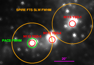
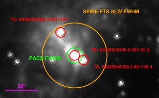
Figure 1: Spitzer 3.6 µm image of N 113 (top) and SAGE 045400.9$-$691151.6 (bottom), identifying the YSO sources (red circles). Also indicated is the PACS beam full-width-at-half-maximum (green circle, $FWHM=9\hbox to0.0pt{.\hss}\arcsec 5$ at the wavelength of the [O i] 63 µm and [O iii] 88 µm lines, Altieri & Vavrek 2013), and the nominal SPIRE FTS beam (orange circle, $FWHM=40\arcsec$ for SLW, Valtchanov 2017). Note that the $FWHM$ for the [C ii] beam is $\sim$ 20% larger. North is to the top and East is to the left.

Figure 1 shows the Herschel pointings with multiple YSO sources: the N 113 region described above (top) and SAGE 045400.9$-$691151.6 and its neighbours (bottom; #7 in Table 1). While resolved in the Spitzer IRAC bands, #7A and 7B are not resolved beyond 24 µm (their separation is approximately 6″); both sources are strong ice sources (Seale et al., 2009, 2011) and are associated with a H₂O maser (Imai et al., 2013). Another nearby source (#7C, separation $\sim$ 20″) is a weak ice source (Seale et al., 2009, 2011). These three sources are unresolved at Herschel SPIRE wavelengths; #7A & 7B are unresolved in the PACS spectra, but a PACS spectrum for #7C could be extracted from the observations (Sect. 3.1). Other sources visible in Fig. 1 (bottom) are relatively blue, for instance they are not detected in the PACS 100 µm images. Henceforth we will refer to unresolved sources #7A & 7B collectively as SAGE 045400.9$-$691151.6. All other pointings are relatively simple point sources at this resolution.

3 Herschel observations and data reduction

The observations discussed here were obtained as part of two Herschel Open Time programmes. These two programmes (proposal identifications OT1$\_$joliveir$\_$1 and OT2$\_$joliveir$\_$2) amounted to 73.4 h of Herschel observing time.

3.1 PACS spectra

All the targets in Table 1 were observed using the PACS spectrometer: an integral field unit made of $5\times 5$ square spaxels – total FOV $\sim$47″ $\times$ 47″) – operating in the 50 $-$ 200 µm range. Selected wavelength ranges were targeted to obtain spectra that include molecular and atomic lines of interest (Table 2). All wavelengths quoted throughout this paper are rest wavelengths in vacuum. The spectral resolution varies between $\lambda/\Delta\lambda$ $\sim$ 3000 (for [O i] at 83 µm) and $\sim$ 1000 (for H₂O at 108 µm).

Table 2: Transitions observed with the PACS spectrometer (line spectroscopy mode). As described in the text, 19 pointings translate to 21 YSO sources resolved with PACS; the last column tallies how many sources are observed for each spectral region (see also Table 1).

Species	Transition	Rest $\lambda(\micron)$	N
[O i]	${}^{3}P_{0}$ – ${}^{3}P_{2}$	63.18	21
OH	${}^{2}\Pi_{1/2}(J=1/2)$ – ${}^{2}\Pi_{3/2}(J=3/2)$	79.11, 79.18	19
OH	${}^{2}\Pi_{3/2}(J=7/2$ – $J=5/2)$	84.4, 84.6	16
[O iii]	${}^{3}P_{1}$ – ${}^{3}P_{0}$	88.36	20
o-H2O	212 – 101	179.52	21
[C ii]	${}^{2}P_{3/2}$ – ${}^{2}P_{1/2}$	157.74	21
o-H2O	221 – 110	108.07	20
CO	14 – 13	185.99	20

The targets are unresolved in all Spitzer and Herschel images, and thus single-pointing mode was used. The emission from the ISM surrounding the targets precluded the use of the chop/nod mode, and instead we observed all targets in unchopped line scan mode, selecting patches of sky with negligible 160 µm emission for the offset measurement (dominated by the emission from the telescope). For this observing mode the continuum level can be recovered in a reliable way only for bright sources (Altieri & Vavrek, 2013); many of our targets are relatively faint in all or some of the observed spectral ranges, therefore continuum uncertainties of at least $\sim$30% are expected. However, both the line profiles and strength are reliably recovered in this observing mode. The number of objects targeted for each PACS range is detailed in the last column of Table 2; ranges not observed for each target are listed in the last column of Table 1.

Spectra were reduced as advised within the Herschel Interactive Processing Environment (HIPE, v.10.0.2, PACS calibration tree version 48) using standard recipes for this type of observations. Reduced observations were retrieved from the database but spectral flatfielding was performed independently step-by-step: this is a crucial task for improving the signal-to-noise ratio (SNR) of the final spectra, and it is advised to monitor the task’s progress closely. For more information, the reader should refer to the “PACS Data Reduction Guide: Spectroscopy”. The spectra were checked against subsequent database, software and calibration releases; no further improvements in the quality of the spectra were forthcoming.

For most pointings the intended target is located in the central spaxel. The spectrum for the central spaxel (2,2) was extracted from the rebinned data cubes (slicedFinalCubes) and a point source flux loss correction was applied (no correction for slight pointing offsets and pointing jitter can be applied to unchopped observations due to the uncertainties in the continuum level). Line flux measurements for the lines of interest (Table 2) were performed on these extracted spectra, using standard spectral fitting tools within HIPE. All lines are spectrally unresolved. Line fluxes for all lines detected with PACS are listed in Table 9; example spectra are shown in Fig. 16.

Referring to Table 1, sources SAGE 045400.2$-$691155.4 and SAGE 045400.9$-$691151.6 (#7A and 7B) are blended as observed with the PACS spectrometer (the observations are actually centred on #7B); these two sources fall on the central spaxel (2,2) while SAGE 045403.0$-$691139.7 (#7C) falls on spaxel (1,3). N 113 YSO-4 was not directly targeted with a separate PACS observation, but it falls onto the FOV of the observations for both N 113 YSO-1 and N 113 YSO-3; this source is however better centred for the observation of N 113 YSO-3, falling on spaxel (4,3). Spectra for those secondary sources are extracted from the spaxels mentioned and the point source flux loss correction is applied; centring on spaxels other than the central one is obviously not optimal, therefore for those sources there are additional flux losses that cannot be corrected for. To summarise, the sample comprises 19 PACS pointings that result in 21 sources for which spectra were extracted. The analysis of all lines detected in the PACS range is described in Section 6.

For some sources, [O i], [C ii] and [O iii] line emission is detected in spaxels other than the central spaxel (see Sect. 6.1.1), i.e. a point source is superposed on an extended environmental contribution. In order to analyse the morphology of the emission region and to estimate the environmental contribution to the on-source line emission, we measured the emission line flux for these lines across all spaxels. Since rebinned data cubes do not have a regular sky footprint (they are organised spatially as a slightly irregular $5\times 5$ grid of 25 spaxels), we projected the data from the irregular native sky footprint onto a regular 3″ sky grid, producing line flux maps (we made use of final data product scripts available within HIPE). Such maps should not be used for science measurements but are adequate to estimate the contribution of the off-source emission. More detail on how these flux maps are used is given in Sect. 6.1.1. When detected, H₂O, OH and CO emission is present only in the central spaxel; compact OH absorption is detected for a small number of sources (see Section 6.2).

3.2 SPIRE FTS spectra

Table 3: Transitions in the SPIRE FTS range.

Species	Transition	Rest $\lambda(\micron)$	Rest $\nu$ (GHz)	$E_{J}$(K)
CO	4 – 3	650.25	461.041	55.30
[C i]	${}^{3}P_{1}$ – ${}^{3}P_{0}$	609.14	492.161	23.62
CO	5 – 4	520.23	576.268	83.00
CO	6 – 5	433.56	691.473	116.20
CO	7 – 6	371.65	806.652	154.90
[C i]	${}^{3}P_{2}$ – ${}^{3}P_{1}$	369.87	809.342	62.46
CO	8 – 7	325.23	921.800	199.10
CO	9 – 8	289.12	1036.912	248.90
CO	10 – 9	260.24	1151.985	304.20
CO	11 – 10	236.61	1267.014	365.00
CO	12 – 11	216.93	1381.995	431.30
[N ii]	${}^{3}P_{1}$ – ${}^{3}P_{0}$	205.18	1461.130	70.10
CO	13$-$12	200.27	1496.923	503.10

We observed our YSO targets using the SPIRE FTS in single-pointing mode with sparse image sampling to obtain spectra from 447 to 1546 GHz ($\sim$ 190 $-$ 650 µm) with spectral resolution $\Delta\nu$ = 1.2 GHz, covering the CO ladder from transitions ¹²CO (4$-$3) to (13$-$12) (Table 3). The full wavelength coverage was achieved by using two bolometer arrays (SPIRE Short/Long Wavelength, respectively SSW and SLW) providing a nominal 2′ unvigneted FOV. In total 19 SPIRE FTS pointings were performed. No SPIRE FTS spectrum is available for N 113 YSO-4; even though it falls within the FOV of the observations of both YSO-1 and YSO-3 (Fig. 1), the positions of the individual SSW and SLW bolometers do not allow for a spectrum to be extracted (see below). Referring to Table 1, a single spectrum was extracted that includes the contributions of sources #7A, 7B and 7C (see also bottom panel in Fig. 1).

FTS spectra were reduced as advised within HIPE  (v.10.0.1, SPIRE calibration tree spire$\_$cal$\_$11$\_$0) using standard recipes for this type of observations (“SPIRE Data Reduction Guide: Spectroscopy”, see also Fulton et al. 2016). Background subtraction was performed using dedicated HIPE scripts; we found that using carefully selected off-axis detectors for the subtraction provided the best results (in terms of spectral shape and agreement between the SSW and SLW bands), compared to using dark sky observations from the same operational day (this is expected for relatively faint sources). The data products were checked against subsequent reprocessings with more advanced HIPE and SPIRE calibration versions for representative sources; no significant improvements were found. Finally the FTS spectra of the targets were extracted from the SLWC3 and SSWD4 detectors. Note that given the nature of the observations (single pointing sparse map), SSW and SLW detector alignment is only achieved for the intended source; thus we cannot extract fully calibrated spectra for other sources in the FOV (e.g., N 113 YSO-4).

The majority of SPIRE FTS spectra show a discontinuity between the SSW and SLW bands. For most sources the discontinuity is such that the SSW flux drops below the SLW flux in the overlap region. This results from the fact that the SLW beam diameter is approximately a factor of 2 larger than that of SSW and it affects any sources that are semi-extended at these wavelengths. For such sources the final spectra are corrected to an equivalent beam size (a Gaussian beam of 40″) using the Semi-extended Correction Tool (SECT, for more details see the “SPIRE Data Reduction Guide: Spectroscopy” already mentioned). It should be noted that there is an implicit assumption that the spatial extension of the continuum and line emitting regions is the same. In total 15 sources out of 19 had a SECT correction applied.

For remaining four sources the discontinuity is reversed, i.e. the SLW flux drops below the SSW flux. This is a calibration effect due to rapidly changing detector temperatures after the cooler was recycled; it affects observations taken at the beginning of an FTS observing block, as is the case for the four sources in question. Specialists at the Herschel Helpdesk reprocessed and corrected the FTS spectra affected.

Line emission intensities were obtained by fitting the unapodised spectra with a low-order polynomial combined with a $sinc$ profile for each line of interest (Table 3), using standard spectral fitting tools within HIPE. Line fluxes for all lines and transitions detected with SPIRE FTS are listed in Table 10; example spectra are shown in Fig. 16. A full characterisation of the SPIRE FTS performance can be found in Hopwood et al. (2015, and references therein), including discussions of line flux and velocity measurements and performance (see also Section 7.1). For four of the 19 SPIRE FTS pointings the SNR for the CO line fluxes (Table 10) is deemed too low for a meaningful analysis (see also Table 1); for these sources we compute total CO luminosities only, and no further analysis is performed. The analysis of emission lines in the SPIRE range (i.e. CO, [N ii] and [C i]) is described in Section 7.

4 Far-IR luminosity and dust temperature

Even though the Magellanic sample was selected trying to avoid sources with a complex background, this was not always the case. We have also found that the Spitzer IRAC and MIPS Magellanic photometric catalogues (Meixner et al., 2006; Gordon et al., 2011) are not always reliable or complete for massive Magellanic YSOs. Such sources are often marginally extended to the extent that they are absent from those point source catalogues (see discussion in Sewiło et al., 2013). Furthermore, massive YSO fluxes at 70 µm often seem anomalously high compared to for instance PACS fluxes. Since aperture photometry has been shown to perform better for samples such as ours (Gruendl & Chu, 2009; Sewiło et al., 2013), we instead performed aperture photometry tailoring the parameters to each source environment. The measured fluxes are presented in Table 8. They are used to estimate the integrated IR luminosity for each target.

Sewiło et al. (2010) described the difficulties of using Spitzer-optimised YSO spectral energy distribution (SED) fitters (e.g., Robitaille et al., 2006) to fit simultaneous Spitzer and Herschel photometry: the model components do not fully account for the envelope of cooler dust and gas further away from the source that emits little at shorter wavelengths but contributes significantly in the Herschel bands. For the line emission analysis presented in this work, it is crucial to constrain the cold dust emission that is the spatial counterpart to the emission lines measured with PACS and SPIRE. The spatial resolution of the observations across the available wavelength range (3.6 $-$ 500 µm) is also very disparate. Improved SED models are available (Robitaille, 2017) but limitations remain; namely only Galactic dust emission without the contribution of PAH emission is included, and a single source of emission is assumed. Since for our analysis we simply require an estimate of the dust temperature and total integrated far-IR emission, we opt instead for the simpler approach of fitting a two temperature component modified blackbody function to the available photometry. A cold blackbody component is responsible for the majority of the far-IR emission (details below), however a hotter component is needed to fit the Spitzer photometry at 24 µm.

To fit the two component modified blackbody we use the blackbody python code, available as part of the agpy collection of astronomical software. It uses a Markov-chain Monte Carlo (MCMC) Bayesian statistical analysis to constrain the modified blackbodies’ temperatures and fluxes; we use an emissivity spectral index $\beta$ = 1.5 (see also Seale et al., 2014). We adopt gas-to-dust ratios of 400 and 1000 (e.g., Roman-Duval et al., 2014), and distances of 50 kpc and 60 kpc (e.g., Schaefer, 2008; Hilditch, Howarth & Harries, 2005), respectively for the LMC and SMC. For further details on the modified blackbody expression and adopted dust opacity $\kappa_{\nu}$ refer to Battersby et al. (2011). Examples of the two component modified blackbody fits are shown in Fig. 15.

Integrated total IR luminosity and cold dust temperature are listed in Table 4; $L(>$ 30 µm) accounts for the majority of the contribution of the cold dust blackbody, while $L(>$ 10 µm) includes the contribution of the warm blackbody; the ratio $L(>$ 30µm)/$L(>$ 10 µm) ranges between 67% and 93% (median 77%). Cold dust temperatures vary between 22 and 39 K (median 31.6 K); the temperature of the warmer blackbody is not well constrained. $L(>$ 10 µm) varies between $\sim$ (5 $-$ 32) $\times 10^{3}$ L_⊙ (median $\sim$ 6.3 $\times 10^{3}$ L_⊙). For the same integrated luminosity there is a tendency for SMC sources to have higher blackbody temperatures, reflecting higher dust temperature (see also van Loon et al., 2010a, b). Seale et al. (2014) determined temperatures and far-IR luminosities for a subset of our sources, using Herschel photometry only. In general the temperatures agree within the uncertainties, but in some cases our derived temperatures are higher given that we took into account additional photometry (70 µm MIPS fluxes are crucial in constraining the dust temperature). The integrated far-IR luminosities from Seale et al. (2014) are in good agreement with our $L(>$ 70 µm) fluxes (not tabulated). In the subsequent discussions we adopt $L(>$ 10 µm) as the object’s total IR luminosity $L_{\rm TIR}$. For these type of objects $L_{\rm TIR}$ does not differ significantly from the bolometric luminosity $L_{\rm bol}$.

Table 4: Parameters for the modified blackbody fits to the available photometry (see Table A1). The emissivity spectral index is $\beta$ = 1.5. Integrated luminosities are tabulated for wavelengths longer than 10 µm and 30 µm, $L(>$10 µm) and $L(>$30 µm) respectively. The temperature of the hotter modified blackbody that contributes to $L(>$10 µm) (see text) is poorly constrained (typically $T$ $\sim$ 100 K). The comments column indicates missing fluxes and provides an empirical assessment of the reliability of the fitted parameters. For LMC053705$-$694741 the tabulated parameters are particularly uncertain: there are two bright sources within $\sim 25$″, and the fit is rather conservative meaning the luminosities could easily be higher by a factor 2. $L(>$10 µm) is adopted as $L_{\rm TIR}$ for all subsequent discussions.

#	Source ID	$T$	$L(>$30 µm)	$L(>$10 µm)	Comments
		(K)	($10^{3}$L⊙)	($10^{3}$L⊙)
SMC YSOs
1	IRAS 00430$-$7326	35.2$\pm$1.4	48.6$\pm$4.1	71.4$\pm$4.8
2	IRAS 00464$-$7322	27.9$\pm$0.6	10.2$\pm$0.6	11.8$\pm$0.6	broad peak, $T$ uncertain
3	S3MC 00541$-$7319	33.5$\pm$2.6	16.1$\pm$1.6	24.1$\pm$1.9	no fluxes available for $\lambda$ $\geq$ 250 µm
4	N 81	31.5$\pm$1.9	41.6$\pm$9.3	53.9$\pm$8.3	poor fit, uncertain parameters
5	SMC 012407$-$73090 (N 88A)	38.1$\pm$2.4	131$\pm$16	195$\pm$25	no fluxes available for $\lambda$ $\geq$ 250 µm
LMC YSOs
6	IRAS 04514$-$6931	32.5$\pm$1.8	55.8$\pm$7.7	68.2$\pm$7.8
7A	SAGE 045400.2$-$691155.4	31.9$\pm$3.3	112$\pm$24	128$\pm$24	flux limits for 70 µm and $\lambda$ $\geq$ 350 µm, extremely uncertain
7B	SAGE 045400.9$-$691151.6
7C	SAGE 045403.0$-$691139.7	35.6$\pm$2.0	76.5$\pm$10	83$\pm$10	flux limits for 70 µm and $\lambda$ $\geq$ 350 µm, extremely uncertain
8	IRAS 05011$-$6815	31.6$\pm$2.1	17.7$\pm$2.1	20.6$\pm$2.3
9	SAGE 051024.1$-$701406.5	23.9$\pm$0.8	12.4$\pm$0.8	18.4$\pm$1.0
10	N 113 YSO-1	30.5$\pm$1.6	217$\pm$21	264$\pm$22	flux limits for $\lambda$ $\geq$ 350 µm
11	N 113 YSO-4	29.7$\pm$3.6	82$\pm$8	114$\pm$8.4	broad peak, $T$ uncertain, uncertain parameters
12	N 113 YSO-3	34.1$\pm$1.9	188$\pm$20	246$\pm$21	flux limits for $\lambda$ $\geq$ 350 µm
13	SAGE 051351.5$-$672721.9	31.8$\pm$1.2	89.5$\pm$8.2	122$\pm$8.9
14	SAGE 052202.7$-$674702.1	25.3$\pm$2.4	24.0$\pm$6.0	28.2$\pm$6.0	flux limits for 70 µm, broad peak, $T$ uncertain
15	SAGE 052212.6$-$675832.4	38.8$\pm$4.0	236$\pm$50	310$\pm$54	$T$ possibly too high
16	SAGE 052350.0$-$675719.6	30.6$\pm$1.0	45.7$\pm$4.4	57.2$\pm$4.5
17	SAGE 053054.2$-$683428.3	33.5$\pm$2.5	55.7$\pm$6.5	72.6$\pm$6.8	flux limits for $\lambda$ $\geq$ 250 µm
18	IRAS 05328$-$6827	22.0$\pm$2.6	9.5$\pm$0.9	12.8$\pm$1.5	flux limits for 70 µm, $T$ uncertain
19	LMC 053705$-$694741	26.1$\pm$4.0	4.6$\pm$1.5	5.0$\pm$1.5	flux limits for 70 µm and $\lambda\geq 350$ µm, extremely uncertain
20	ST 01	29.8$\pm$2.1	33.1$\pm$3.6	40.5$\pm$3.7	broad peak, flux limits for $\lambda$ $\geq$ 250 µm, $T$ uncertain

5 Galactic massive YSO comparison sample

One of the challenges in observing and interpreting the data of massive YSOs in the Magellanic Clouds lies with the fact that observations probe different spatial scales compared to Galactic massive YSOs. A sample of high luminosity Galactic YSOs was observed with Herschel (Karska et al., 2014), however the spatial scales probed (corresponding to the central PACS spaxel only) sample very different spatial components in the massive YSO environment compared to the Magellanic Herschel observations. Furthermore, the [C ii] emission is often saturated for those sources. With this in mind, we instead compiled a Galactic comparison sample of massive YSOs observed with the Infrared Space Observatory (ISO, Kessler et al., 1996). In fact, the region sampled by PACS at 156 µm at a distance of the LMC ($\sim$ 50 kpc) is equivalent to the region sampled by the ISO Long-Wavelength Spectrograph (ISO LWS, Clegg et al., 1996) at a distance of $\sim$ 8 kpc (ISO-LWS equivalent beam size information from Gry et al. 2003).

We identified 22 massive YSOs observed with ISO LWS with luminosities in the range $\sim$ (5$-$500) $\times 10^{3}$ L_⊙ and located at distances in the range $\sim$ 1$-$10 kpc (see Table 11 for individual object information); the spectra of these sources were retrieved from the ISO Data Archive(IDA). Of these 22 spectra we selected 19 for which both the [O i] and [C ii] lines are in emission. The relatively low SNR of the spectra, especially at shorter wavelengths, implies we were only able to measure fluxes for the strongest emission lines: [C ii] at 158 µm, [O i] at 63 and 145 µm, [O iii] at 88 µm, [N ii] at 122 µm and CO at 186 µm. To ensure uniformity in the way fluxes are estimated, we measured all line fluxes from archival spectra rather than using published measurements. More details on this massive YSO comparison sample are provided in Appendix E. The Magellanic and Galactic sample properties are further discussed in Sect. 8.2.2.

6 Results: PACS spectra

6.1 [C ii], [O i] and [O iii] emission

6.1.1 Emission line morphology

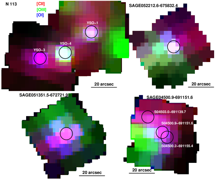
Figure 2: Line emission maps for [C ii] (red), [O iii] (green) and [O i] (blue). The YSOs in N 113, SAGE 052212.6$-$675832.4, SAGE 045400.9$-$691151.6 and SAGE 051351.5$-$672721.9 (clockwise from top left) are shown (black circles with diameter 9.″5, the $FWHM$ of the [O i] and [O iii] beams). North is to the top and East to the left in all maps.

[C ii], [O i] and [O iii] emission is often detected beyond the central spaxel. [C ii] emission is usually present across the FOV, covering it completely for all but two sources. [O i] emission completely covers the FOV in 11 out of 19 pointings, and is present beyond the central spaxel in eight others. Crucially there is always a flux enhancement in the central spaxel related to the point source targeted, i.e. the point source contribution is superposed on extended diffuse environmental emission.

We investigate the morphology of the extended emission lines observed, making use of the line emission maps described in Sect. 3.1. Taking into account the beam size for each line, these maps are used to estimate the environmental contribution as a fraction of the peak flux at the source position; that contribution is subtracted from the measured line flux for the source, and a point source correction is applied (Sect. 3.1). For [O i] the environmental emission accounts for typically 20% (maximum 70%) in the LMC and 7% (maximum 11%) in the SMC; for [C ii] it accounts for typically 42% (maximum 85%) in the LMC and 30% (maximum 50%) in the SMC. Clearly the extended diffuse contribution is more important for [C ii] emission than for [O i] emission (see also Lebouteiller et al., 2012), but it is also more significant for LMC sources compared to SMC sources. Furthermore, the morphology of the [C ii] and [O i] extended emission follows the dust emission (e.g., 100 µm PACS emission), even if the [O i] emission is generally less extended (Fig. 2).

The [O iii] emission line morphology is as expected somewhat different, given its distinct physical origin (see discussion in next section). Out of the 18 observations in this spectral range (IRAS00464$-$7322 was not observed), six sources are not detected in [O iii] line emission and four sources exhibit compact emission at the central spaxel only. For the other eight pointings, emission extends across the FOV: for two of these the intended target (that falls on the central spaxel) is the source of the strongest emission; we discuss below the remaining six pointings in more detail.

As can be seen in Fig. 2 (top left), for the two pointings in N 113, YSO-1 and YSO-4 are strong [O iii] emission line sources, while YSO-3 is actually consistent with environmental emission or contamination from YSO-4 (the strongest [O iii] emitter in this region). Strong emission also originates from locations at the FOV’s northern and western edges. For four other pointings the peak [O iii] emission is displaced from the central spaxel. Figure 2 (bottom right) shows the line emission in the region of SAGE 045400.9$-$691151.6. While the spatial distributions of [O i] and [C ii] emission are similar (tracing the dust emission), the [O iii] emission is clearly offset. This morphology is very suggestive of a large ionised gas bubble (as seen also in MCELS images) with the three YSOs embedded in the dust at its rim. The observed emission for SAGE 045400.9$-$691151.6 and N 113 above are reminiscent of the emission line maps of LMC-N 11, in which the spatial distribution of [O iii] emission seems anti-correlated to that of [C ii] (Lebouteiller et al., 2012).

Two other sources with off-source [O iii] peak emission are also shown in Fig. 2: SAGE 051351.5$-$672721.9 (bottom left) and SAGE 052212.6$-$675832.4 (top right) are also detected in the MCELS [O iii] map. While there might be a slight problem with source centring on the spaxel, it is nevertheless very clear that the [O iii] emission is not point-source like. Instead it originates from the immediate surrounding H ii regions: SAGE 051351.5$-$672721.9 is situated $\sim$20″ from the ionising B[e] supergiant Hen S22 (Chu et al., 2003), while SAGE 052212.6$-$675832.4 is just $\sim$10″ away from an O7V star within N 44C (Chen et al., 2009). Therefore we conclude that the observed emission for SAGE 051351.5$-$672721.9 and SAGE 052212.6$-$675832.4, as well as N 113 YSO-3 and SAGE 045400.9$-$691151.6 above, is likely mostly ambient.

A final source, SAGE 053054.2$-$683428.3 (not shown in Fig. 2), exhibits compact [O iii] emission centred on spaxel (2,3) superposed on more extended environmental emission. Inspection of the emission line centroids for several spaxels reveals wavelength shifts that are a tell-tale sign that the source is not well centred in the central spaxel and is offset in the dispersion direction (i.e. from spaxel (2,2) to spaxel (2,3), for more details refer to Vandenbussche, 2011). Thus, the observed compact [O iii] emission is very likely associated with the source on the central spaxel but it is affected by poor source centring.

In brief, [O iii] emission associated with the YSO targets is detected for a total of nine sources, six in the LMC and three in the SMC.

6.1.2 Emission line diagnostics and correlations

In this section we compare line emission for [C ii], [O i] and [O iii]  for the Magellanic sample and the Galactic ISO sample. Emission lines like [O i] and [C ii] are often used to diagnose the environmental conditions of massive YSOs, since they are amongst the main contributors to line cooling. The difficulty is that such lines can originate from distinct components within the star formation environment. In particular in their later evolutionary stages, massive YSOs are copious producers of ultraviolet photons; as a result they often exhibit expanding compact H ii regions, even while still actively accreting from their envelopes (e.g., Beuther et al., 2007). These emerging H ii regions help shape the structure and chemistry of the YSO environment. In schematic terms (see Kaufman, Wolfire & Hollenbach, 2006, for an actual diagram and further details), two main regions can be distinguished: the H ii region itself marks the sphere of influence of H-ionising photons ($h\nu$ $\geq$ 13.6 eV); less energetic far-untraviolet (FUV) photons (6 eV $\leq$ $h\nu$ $\leq$ 13.6 eV) penetrate into the adjacent neutral and molecular hydrogen gas and play a significant role in the chemistry, heating and ionisation balance of these photodissociation regions (e.g., Tielens & Hollenbach, 1985). PDRs include both the neutral dense gas near the YSOs but also the neutral diffuse ISM. Energetic outflows are also a ubiquitous phenomenon in massive star formation, driving shocks through the surrounding gas (e.g., Beuther et al., 2007; Bally, 2016). Both PDRs and shocks contribute to the excitation of far-IR [O i], [C ii] and CO emission (e.g., Hollenbach & McKee, 1989; Kaufman et al., 1999, 2006), while shocks are particularly important to H₂O and OH excitation (e.g., van Dishoeck et al., 2011; Wampfler et al., 2013).

The ionisation potential for neutral carbon C⁰ is just 11.26 eV, therefore [C ii] emission can originate not only in H ii regions, but also in PDRs and diffuse atomic and ionised gas (e.g., Kaufman et al., 1999, 2006). On the other hand, [O i] is only found in neutral gas (the ionisation potential for O⁰ is 13.62 eV, just above that for hydrogen), and emission arises from warm, dense regions. [O i] emission can originate from deeper inside the PDR than [C ii] since some atomic oxygen remains in regions where all carbon is locked into CO. [O i] emission also originates from shocks in molecular outflows that can contribute in a small fraction to [C ii] emission (resulting in [O i]/[C ii] flux ratios of $>$ $\sim$  10, Hollenbach & McKee, 1989). Given the relatively high ionisation potential for O⁺ (35 eV), [O iii] emission originates from H ii regions, rather than the diffuse interclump medium (e.g., Cormier et al., 2015, for a thorough description of these line properties). We note that the ionised gas emitting [O iii] emits little [C ii] (the ionisation potential for C⁺ is 24.38 eV); ionised [C ii]-emitting gas is traced instead by [N ii] emission (the ionisation potential for N⁰ is 14.53 eV).

It is important to quantify the contribution of ionised gas to [C ii] emission, before comparing [C ii] and [O i] line fluxes. Considering an integrated PDR and H ii region model, Kaufman et al. (2006) find that for solar metallicity [C ii] emission is always dominated by the PDR contribution as opposed to the contribution of the ionised gas in the H ii region; furthermore the H ii region contribution increases for higher metallicity environments. As described in Sect. 7.5.1, we estimated the ionised gas contribution to [C ii] for the eleven Magellanic YSOs for which [N ii] 205 µm emission is detected with the SPIRE FTS; this contribution is typically $\sim$ 20%. For the Galactic sample, we detect [N ii] emission at 122 µm for seven out of 18 sources; the ionised gas contribution is $\sim$ 40% (Appendix E). These contributions are consistent with other estimates available in the literature, and with an increased contribution for high metallicity environments (further discussion in Sect. 7.5.1).

As mentioned in Sect.6.1.1, for the Magellanic sample we corrected the [O i] and [C ii] line fluxes for the contribution of more extended diffuse gas; the [C ii] ionised gas correction is generally smaller than the extended gas contribution. We do not have extended gas estimates for the Galactic sample; however this would tend to enhance the observed differences between the Magellanic and Galactic samples (see discussion below and Figs. 3 and 4).

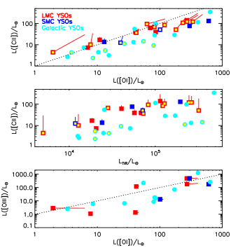
Figure 3: FIR line correlations: [C ii] versus [O i] luminosities (top panel), [C ii] luminosity versus $L_{\rm TIR}$ luminosity (middle) and [O iii] versus [O i] luminosities (bottom). Squares represent Magellanic YSOs (respectively red and blue for the LMC and the SMC) and circles represent Galactic YSOs. Line luminosities for both samples have been corrected for the ionised gas contribution to [C ii] emission (for sources with [N ii] emission (yellow symbols), see text). Only the Magellanic sample has been corrected for contribution of the extended diffuse emission (see text for details); the colour-coded lines indicate the size of this correction.

In Fig. 3 we compare [C ii], [O i] and TIR luminosities for the Magellanic and Galactic samples. Firstly, for both samples the [O i] and [C ii] luminosities are strongly correlated (top panel, Spearman’s rank correlation $\rho\sim 0.89$ and the probability that the two quantities are uncorrelated is $p<10^{-6}$). Even though [O i] emission at 63 µm can be affected by optical depth effects, this strong correlation suggests a common origin for the majority of the emission being measured. Secondly, [C ii] luminosity correlates with the YSO’s $L_{\rm TIR}$ emission (middle panel, $\rho\sim 0.81$, $p<10^{-5}$) indicating that photons from the YSO are responsible for its excitation. Furthermore, the [O i]/[C ii] flux ratios are relatively low ($\sim 0.3-5$) suggesting negligible contribution from shock excitation (Hollenbach & McKee, 1989). Put together, this points to both [C ii] and [O i] emission originating predominantly from a PDR component, at the spatial scales sampled here (i.e. “integrated” over the whole complex YSO environment). The ratio [O i]/[C ii] correlates with line emission, more strongly with [O i] than [C ii] emission (Spearman’s $\rho$ respectively 0.86 and 0.56). This is likely related to uncertainties in the large corrections for the diffuse emission. Fig. 3 also shows that the line emission to dust continuum ratio is typically higher in the Magellanic Clouds compared to the Galaxy (by a factor $\sim 4.5$ for $L($[C ii])/$L_{\rm TIR}$ and $\sim 3.5$ for $L($[O i])/$L_{\rm TIR}$, comparing line luminosities uncorrected for extended emission contribution), as seen also for instance by Israel & Maloney (2011, and references within).

Figure 3 (bottom) shows that the Magellanic and Galactic samples are not significantly distinct in terms of [O iii] emission: the mean $L($[O iii]$)/L($[O i]$)$ ratio uncorrected for diffuse emission is $\sim$ 1 with a large scatter for both samples. This is broadly consistent with a typical ratio of $\sim$ 0.8 measured for another sample of Magellanic YSOs using Spitzer MIPS spectroscopy (van Loon et al., 2010a, b). As described in Sect. 6.1.1, the emitting regions are complex and extended, and it is not always clear what is the origin of the [O iii] emission. There is a weak correlation between [O iii] and [O i] and [C ii] emission, suggesting a mild luminosity scaling effect. The $L($[O iii]$)/L($[O i]) ratio can be a probe of the filling factor of ionised gas compared to that of the PDR gas. In dwarf galaxies and resolved Magellanic star forming regions (SFRs), this ratio is high ($\sim$ 3, Cormier et al., 2015, see also Jameson et al. 2018). However, such discussion of relative filling factors of different gas phases is likely only meaningful over large scales of whole SFRs or unresolved galaxies, not on smaller YSO scales (i.e. on the scales of a single PACS spaxel).

6.1.3 Photoelectric heating efficiency

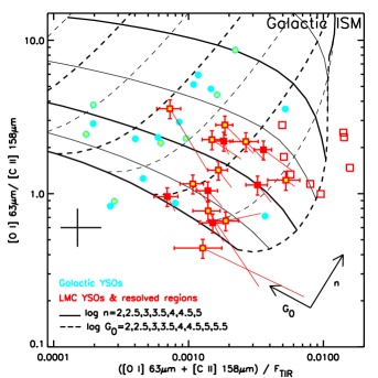
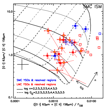
Figure 4: PDR diagnostic diagram using [C ii], [O i] and $F_{\rm TIR}$ fluxes, for Galactic and LMC sources (top) and LMC and SMC sources (bottom). Plotting symbols are as in Fig. 3; open squares are resolved SFRs in the Magellanic Clouds (Cormier et al., 2015). The black cross gives the size of 25% systematic uncertainties. For the Magellanic sources corrections for the ionised [C ii] gas fraction and extended emission are applied; for the Galactic sources only an ionised [C ii] fraction correction is applied (see text for further details). Observations are compared to models from the PDR Toolbox (Kaufman et al., 1999, 2006), for Galactic ISM conditions (top) and adapted for SMC ISM conditions (Jameson et al., 2018).

Figure 4 shows the traditional PDR diagram used to diagnose emitting gas conditions, i.e. line ratio [O i]/[C ii] versus the total line fluxes compared to the total TIR emission ([O i]+[C ii])/$F_{\rm TIR}$. The line emission is unresolved, therefore we implicitly assume that the beam filling factor is the same for both emission lines. The Galactic and Magellanic YSOs have been corrected for the contribution of ionised gas to [C ii] emission, and Magellanic YSOs have further been corrected for the contribution of more diffuse extended gas (corrections shown in Fig. 4). It is clear that the YSO samples occupy different regions in this diagram: similar line ratios are observed, but the line emission is more prominent in the Magellanic Clouds for the same dust emission as measured by TIR emission, compared to Galactic sources.

We also include a sample of resolved Magellanic SFRs (Cormier et al., 2015), for which line and dust emission fluxes are summed over the whole regions mapped. Line intensity and ratios vary across the regions mapped; furthermore the fraction of line intensity compared to dust emission decreases from the diffuse medium to denser regions in SFRs (in the LMC, Rubin et al., 2009). Therefore the massive YSO sample has weaker line emission relative to dust emission when compared to integrated SFRs (see also Jameson et al., 2018). As described in Chevance et al. (2016), $F_{\rm TIR}$ can also include a contribution from ionised gas; such contribution is traced for instance by the [O iii] emission. We find that the ([O i]+[C ii])/$F_{\rm TIR}$ ratio is not anticorrelated with the [O iii]/[C ii] ratio, as would be expected if a significant fraction of $F_{\rm TIR}$ resulted from the ionised gas contribution. Therefore, we conclude that $F_{\rm TIR}$ is mostly tracing dust cooling.

The ratio ([O i]+[C ii])/$F_{\rm TIR}$ is often used as a proxy for the photoelectric heating efficiency. Dust grains absorb incident radiation and emit electrons that in turn heat the gas; given that [O i] and [C ii] are the main coolants in dense PDRs, and far-IR continuum emission (as well as PAH emission) cools the dust, this ratio provides a measure of the efficiency of the photoelectric heating (e.g., Kaufman et al., 1999). From Fig. 4 this efficiency is higher for Magellanic YSOs when compared to Galactic YSOs, with medians respectively 0.25% and 0.1%, with a large scatter. These estimates are broadly consistent with other estimations in the Galaxy (e.g., Salgado et al., 2016) and the Magellanic Clouds (van Loon et al., 2010b). There seems to be no clear difference between the LMC and SMC samples (as found also by van Loon et al., 2010b). The photoelectric heating efficiency can be enhanced if the grains are less positively charged, leading to more, and more energetic, electrons being released. Indeed Sandstrom et al. (2012) and Oliveira et al. (2013) suggested that observed PAH emission ratios in the SMC are consistent with a predominance of small neutral PAHs.

In Fig. 4 we also compare the YSO ratios with the PDR model predictions  from the PDR Toolbox (Kaufman et al., 1999, 2006). The emission is parameterised in terms of the cloud density $n$ and the strength of the FUV radiation field $G_{0}$ (in units of the Habing Field, 1.6 $\times$ $10^{-3}$ ergs cm^-2 s^-1). We show two sets of PDR models: for standard Galactic conditions (top) and using modified grain extinction, grain abundances, and gas-phase abundances appropriate for SMC ISM conditions (bottom, full details can be found in Jameson et al., 2018). Figure 4 suggests that the range of parameterised densities is similar ($n$  $<$ $\sim$  1 $-$ 3 $\times 10^{4}$ cm^-3), however the Magellanic YSOs are consistent with lower values of $G_{0}$ ($G_{0}$  $<$ $\sim$  2 $\times 10^{3}$, bottom), i.e. weaker radiation field at the surface of the PDR, when compared to Galactic YSOs ($G_{0}$  $>$ $\sim$  1 $\times 10^{3}$, top). Therefore the $G_{0}/n$ ratio is lower for Magellanic YSOs.

From a study of low metallicity dwarf galaxies, Cormier et al. (2015) interpreted lower $G_{0}/n$ ratios as an indication of a change in ISM structure and PDR distribution. Very schematically, low-metallicity H ii regions fill a larger gas volume meaning that PDR surfaces are at larger average distances from the FUV source, effectively reducing $G_{0}$. The mean free path of UV photons is longer (UV field dilution, see also Madden et al., 2006; Israel & Maloney, 2011) leading to reduced grain charging. There is also evidence that the ISM is more porous in lower metallicity galaxies (Madden et al., 2006; Cormier et al., 2015), allowing ionising radiation to more easily leak into pristine ISM. This would imply that the region of influence for massive YSOs in the Magellanic Clouds is generally larger with important consequences for feedback processes (Ward et al., 2017). Our analysis lends support to distinct ISM properties at lower metallicity also on scales of a few parsecs.

6.2 Other lines in the PACS range

In this section we discuss other lines detected in the PACS spectra. While atomic line emission seems to originate predominantly from PDRs, H₂O and OH emission originates from shocks impacting on dense protostellar envelopes in complex YSO environments (e.g., van Dishoeck et al., 2011; Wampfler et al., 2013), with some contribution from outer, more quiescent envelopes to ground-state H₂O emission (van der Tak et al., 2013). The origin of CO emission in either PDRs or shocks is discussed in the next section.

6.2.1 H₂O lines

For our sample of 21 sources with PACS spectra all sources were observed in the range that includes the H₂O line at 179.5 µm, and all but one SMC source (IRAS 00464$-$7322) were observed in the range that includes the H₂O line at 108 µm (Tables 1 and 2); the H₂O 180.5 µm line falls too close to the edge of the spectrum to be usable. In the LMC six sources exhibit H₂O emission; in the SMC there is only one source with a tentative H₂O emission detection. H₂O absorption is not detected in the spectra of any LMC or SMC source.

In the LMC sample the following sources exhibit 179.5 µm H₂O emission: N 113 YSO-1, N 113 YSO-3, N 113 YSO-4, IRAS 05011$-$6815 (all H₂O maser emitters, e.g., Imai et al. 2013), and IRAS 04514$-$6931 (YSO with strong 15 µm CO₂ ice absorption in its Spitzer-IRS spectrum, from which strong H₂O ice absorption can be inferred, Oliveira et al. 2009). The remaining LMC H₂O maser source in the sample, SAGE 045400.9$-$691151.6 (#7A&B in Table 1), exhibits no detectable H₂O emission lines, but another source in that protocluster, SAGE 045403.0$-$691139.7 (#7C) does. N 113 YSO-3 is the only source with definite H₂O emission both at 179.5 and 108 µm. Towards the H₂O maser source in the SMC (IRAS 00430$-$7326, Breen et al. 2013) emission at 108 µm is tentatively detected. Spectra are shown in Fig. 17.

Karska et al. (2014) analysed PACS range spectroscopy (55 $-$ 190 µm) for ten Galactic massive YSOs, covering a range of luminosities $\sim$ (1$-$5)$\times 10^{4}$ L_⊙ (see their Table 1). All but two sources in that sample show a combination of H₂O emission and absorption lines; two sources show H₂O absorption lines only. Only W3 IRS5 exhibits 179.5 µm emission, accounting for less than 2% of the total H₂O line emission. This source is one of the most evolved in the Karska et al. (2014) sample, and it is also one of the sources with the largest contribution of H₂O luminosity to the total molecular cooling in the PACS range ($\sim$ 35%, corresponding to $\sim$ 30% of the total, atomic and molecular, line cooling). W3 IRS5 also exhibits H₂O maser emission and ice absorption features (Gibb et al., 2004, and references therein).

More recently, Karska et al. (2018) analysed a large sample of low-luminosity Galactic YSOs. All sources exhibit H₂O emission; 55% of the sources show emission at either 179.5 or 108 µm (see also Karska et al., 2013; Mottram et al., 2017). The 179.5 µm line accounts for $\sim$ 8% of the total H₂O luminosity with a large scatter (Karska et al., 2013, 2018). Typically the ratio of 179.5 µm to 108 µm emission is $\sim$ 0.9 (range 0.6 $-$ 1.3, Karska et al., 2013), therefore both lines together account for $\sim$ 18% of the total H₂O line luminosity. These fractions will be used in Sect. 8.2 to estimate the total H₂O line luminosity for the Magellanic sample.

6.2.2 OH lines

The full sample of 21 sources with PACS spectra was observed in spectral ranges that cover at least one of the OH doublets listed in Table 2: for twelve LMC and two SMC sources we have spectra for both OH doublets at 84 and 79 µm; for a further four LMC and three SMC sources we have observations for only one doublet (see Table 1). For the 84 µm doublet, we have detected emission for the bluest component (84.4 µm) for two sources: N 113 YSO-3 and IRAS 04514$-$6931; no absorption features are detected. For the 79 µm doublet, two sources exhibit weak absorption (SAGE 052350.0$-$675719.6 and SAGE 052212.6$-$675832.4), three sources show emission (N 113 YSO-3, N 113 YSO-4 and SAGE 045400.9$-$691151.6), and N 113 YSO-1 shows emission for the bluest component (79.11 µm) only. Most sources that show OH emission exhibit H₂O emission (the exception is SAGE 045400.9$-$691151.6). No OH emission or absorption is detected for SMC targets. Spectra are shown in Fig. 18.

Referring to the Karska et al. (2014) study of Galactic massive YSOs, while most sources show some OH emission, the OH doublets at 84 µm and 79 µm are seen mostly in absorption for most sources. This is in contrast with low- and intermediate-mass YSOs, for which these OH doublets are seen mostly in emission, e.g., 63% sources show the 84 µm doublet in emission (Karska et al., 2018). Based on the samples described in Wampfler et al. (2013), the typical flux ratios are F(79.11)/F(79.18) $\sim$ 1.0 (range 0.6 $-$ 1.8) and F(84.42)/F(84.60) $\sim$ 1.34 (range 0.8 $-$ 2.9) for the doublet components, F(79.18)/F(84.42) $\sim$ 0.7 (range 0.3 $-$ 0.86), and F(79)/F(84) $\sim$ 0.77 (range 0.4 $-$ 1.23). In terms of fraction of total OH luminosity, the 79 and 84 µm doublets account for $\sim 24$% and $\sim 31$%, respectively.

The observed ratios for the Magellanic sources are consistent with the values above, with large uncertainties. Where only one doublet component is detected, the upper limits are also consistent with these ratios. We take the estimated luminosity fractions above to predict total OH luminosities from our measured line fluxes. We will discuss the emission line budget for the LMC and SMC sources in Section 8.2.

6.2.3 CO (14$-$13) line emission

We only detected CO (14$-$13) emission for eight sources (out of 19 sources observed); since we detected CO emission lines in the SPIRE range for all sources (see next section), this is probably just due to the low SNR ratio of the PACS spectra. Given the very different beam sizes for PACS and SPIRE and the fact that the emission beam filling factor is unconstrained, our analysis of the CO rotational diagram is based solely on those lines in the SPIRE spectral range.

7 Results: SPIRE FTS spectra

Table 1 provides an overview of the SPIRE FTS observations. One source in the sample was not observed with this instrument mode. A further four sources (three in the LMC and one in the SMC) resulted in FTS spectra with low continuum and line SNR ($<5$ for all CO ladder transitions); for those sources we only compute the total CO luminosity $L_{\rm CO}$ but we are not able to reliably identify other emission lines nor analyse the CO rotational diagrams. That leaves fifteen sources that are discussed in more detail in this section.

7.1 Line identifications

While most CO ladder transitions for these fifteen sources are usually well identified and measured, the process is somewhat more complicated for weaker emission lines that are detected at generally lower SNR, as is the case for the [C i] and [N ii] lines (Table 3). As described in Hopwood et al. (2015), the SNR ratio below 600 GHz is significantly diminished and this strongly impacts on the measured centroid line position (derived from $sinc$ profile fitting, see Section 3.2) for individual transitions (see their Fig. 16). Note that the line emission SNR for the point-source stellar calibrators discussed in the Hopwood et al. (2015) analysis is typically much higher than the SNR for all line detections discussed here (at most we achieve SNR $\sim$ 40).

We measured the variation of the centroid velocity position for the CO line emission for our sample; typical values are $\sim$ 40 km s^-1 and $\sim$ 70 km s^-1 for sources with typical SNR larger and smaller than 10, respectively (the median velocity is always consistent with the typical systemic velocity of the LMC and SMC, $\sim$ 250 km s^-1 and $\sim$ 160 km s^-1 respectively). Even for spectra with the highest SNR overall (N 113 YSO-1, SNR = 22 $-$ 41), the velocity position for the CO (4$-$3) line at 461.041 GHz deviates by $\sim$ 3-$\sigma$ from the median centroid velocity for the other nine CO lines.

The [C i] line at 492.161 GHz is especially affected by these uncertainties in the centroid line position. After careful inspection, we consider this line to be appropriately detected if SNR $\geq$ 5 and the velocity position is consistent with that of the nearest CO lines; this is the case for five LMC sources and one SMC source. The other [C i] line at 809.342 GHz is detected for all sources except for one SMC source (#4, N 81). The [N ii] line at 1461.13 GHz is located in a more favourable part of the spectrum (better continuum SNR); this line is detected (SNR $\geq$ 5) for nine LMC and two SMC sources. These emission lines are further discussed in Sect. 7.5.

7.2 Total CO luminosity measured over the SPIRE range

In Fig. 5 we plot the total CO luminosity $L_{\rm CO}$ measured over the SPIRE range – CO (4$-$3) to CO (13$-$12) – against $L_{\rm TIR}$; there is a strong correlation between the two luminosities: the Spearman’s rank correlation is $\rho=0.74$ and the probability that the two quantities are uncorrelated is $p<0.0016$. Since the energy that heats the gas derives in some form from the YSO, such correlation is not unexpected. There is no correlation between $L_{\rm CO}$ and the dust temperature. These findings are consistent with results for low-luminosity Galactic samples (Manoj et al., 2013, 2016; Yang et al., 2018). Typically $L_{\rm CO}/L_{\rm TIR}$ is $\sim$ 0.06% and $\sim$ 0.02% for the LMC and SMC sources respectively, with a large scatter. There is a tendency for SMC sources to be weaker CO emitters. The LMC $L_{\rm CO}/L_{\rm TIR}$ ratio is consistent with that found by Lee et al. (2016) across their SPIRE CO maps for the SFR N 159W, $L_{\rm CO}/L_{\rm TIR}$ $\sim$ 0.08%.

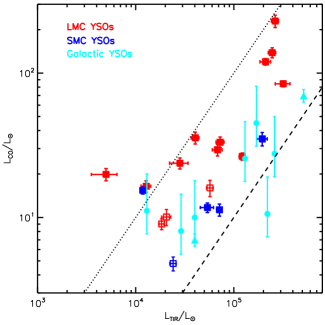
Figure 5: $L_{\rm CO}$ measured over the SPIRE range (4 $\leq$ $J$ $\leq$ 13) versus $L_{\rm TIR}$ for all sources. Filled squares represent the fifteen Magellanic YSOs with fitted CO rotational diagrams (Sect. 7.3), otherwise open squares are used. $L_{\rm CO}$ for massive Galactic YSOs are estimated from CO (14$-$13) ISO fluxes, with the exception of two literature measurements (triangles, Stock et al., 2015). Ratios $L_{\rm CO}/L_{\rm TIR}$ of 0.1% (dotted line) and 0.01% (dashed line) are shown; the latter is the limit proposed for shock-dominated heating (Meijerink et al., 2013), see Sect. 7.4.

For the massive Galactic comparison sample observed with the ISO-LWS, CO (14$-$13) fluxes were measured for seven YSOs (Sect. 5 and Table 11). For the eight Magellanic sources with PACS CO (14$-$13) measurements (Sect. 6.2.3), we estimate a typical fraction $L($CO(14$-$13))/$L_{\rm CO}$ $\sim$ 0.12 $\pm$ 0.06. This is consistent with a ratio $L($CO(14$-$13))/$L_{\rm CO}$ $\sim$ 0.09 $\pm$ 0.04 measured for a larger sample of Galactic sources (Green et al., 2016; Yang et al., 2018). Accordingly, we adopt $L($CO (14$-$13))/$L_{\rm CO}$ = 0.09 to estimate $L_{\rm CO}$ for the seven Galactic YSOs. The $L_{\rm CO}/L_{\rm TIR}$ ratio for Galactic sources is $\sim$ 0.02%, consistent with measurements for two Galactic sources (Stock et al., 2015). The CO luminosities for the Magellanic and Galactic samples are broadly consistent. However, the Galactic ratio is closer to that of the SMC sample, and the LMC sources tend to exhibit higher ratios. Nevertheless, this suggests that the correlation between $L_{\rm CO}$ and $L_{\rm TIR}$ (or $L_{\rm bol}$) extends from low-luminosity YSOs (Manoj et al., 2016; Yang et al., 2018) to massive YSOs, supporting a common origin for the observed CO emission.

Using data available in the literature (e.g., Stock et al., 2015; Green et al., 2016; Yang et al., 2018) we estimate that $L_{\rm CO}$ measured over the SPIRE range (4 $\leq$ $J$ $\leq$ 13) is about 52% of the total CO luminosity measured over the Herschel range ($J$ $\geq$ 4), with a large scatter.

7.3 CO rotational diagram analysis

When multiple rotational transitions are available, the analysis usually relies on the so-called molecular rotational diagrams (e.g., Goldsmith & Langer, 1999), where the logarithm of the total number of molecules in the upper state of a transition $N_{J}$ normalised by the degeneracy of the level $g_{J}$ is plotted against the upper level excitation energy $E_{J}$. In this section we analyse the CO rotational diagrams for the fifteen sources with adequate SNR (eleven in the LMC and four in the SMC); we consider optically thin gas components in local thermodynamic equilibrium (LTE), and subthermally excited (non-LTE) gas.

7.3.1 Optically thin LTE gas models

If the CO emission is optically thin, the total number of molecules in the upper state of a transition $N_{J}$ is related to the observed line flux $F_{J}$ as follows:

$$N_{J}=4\pi d^{2}\frac{F_{J}}{h\nu_{J}A_{J}},$$ (1)

where $\nu_{J}$ and $A_{J}$ are respectively the frequency and Einstein coefficient for the transition, and $d$ is the distance to the source (we adopt $d_{\rm LMC}=50$ kpc and $d_{\rm SMC}=60$ kpc throughout this work). These population levels follow a Boltzmann distribution:

$$\frac{N_{J}}{g_{J}}=\frac{N_{\rm CO}}{Q}e^{-E_{J}/T_{\rm rot}},$$ (2)

where $N_{\rm CO}$ is the total number of molecules, $Q=kT/hcB$ is the partition function for linear molecules ($B=192.25$ m^-1 for CO), $E_{J}$ and $g_{j}$ are the upper level energy (in K) and degeneracy respectively, and $T_{\rm rot}$ is the rotational temperature. Assuming the density is high enough to thermalise all relevant energy levels ($n\geq 10^{6}$ cm^-3 for $J$ = 4$-$13, Yang et al., 2010), $T_{\rm rot}$ is the kinetic temperature $T$ of the gas for all transitions, and values for $T$ and $N_{\rm CO}$ can be simply determined from the slope and intercept of the rotational diagram. If the levels are not thermalised then $T_{\rm rot}$ < $T$ (e.g., Goldsmith & Langer, 1999) and the true value of $T$ is underestimated; furthermore the calculated partition function $Q$ (a function of $T$) is too small and consequently $N_{\rm CO}$ is overestimated. If some transitions are optically thick, non-linear effects are introduced in the rotational diagram (e.g., Goldsmith & Langer, 1999). Non-LTE and optical depth effects are discussed subsequently.

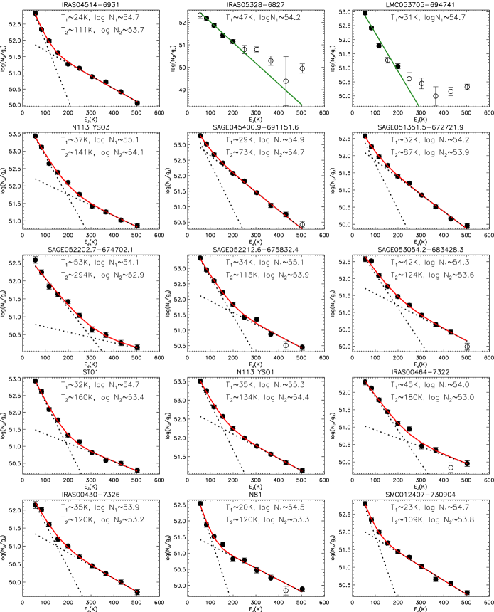
Figure 6: CO rotational diagrams for the Magellanic YSO sample (open symbols indicate data points with SNR < 5). The transitions measured over the SPIRE range are CO (4$-$3) to CO (13$-12$). The characteristic break in the rotational diagrams suggests the presence of two isothermal LTE components with different temperatures $T_{i}$ and total number of CO molecules $N_{i}$ (red lines; the dashed lines show the contributions of the individual components); for two sources only a cold component is fitted for $J$ $\leq$ 9 (green lines). Approximate best fit values appear in each panel; fitted parameters with uncertainties are listed in Table 5.

Table 5: LTE fit parameters to the observed CO rotational diagrams (CO (4$-$3) to CO (13$-12$)), using two isothermal gas components with different temperatures $T_{i}$ and total number of CO molecules $N_{i}$. For IRAS05328$-$6827 and LMC 053705$-$694741 a single isothermal component is fitted ($J$ $\leq$ 9); for SAGE 052202.7$-$674702.1 the properties of the warmer component are poorly constrained. Also listed are $\chi^{2}$ and number of degrees of freedom $N_{\rm f}$ for each fit.

Source ID	$T_{1}$	$\log N_{1}$	$T_{2}$	$\log N_{2}$	$\chi^{2}$	$N_{\rm f}$
	(K)	(mol)	(K)	(mol)
LMC YSOs
IRAS 04514$-$6931	24.2$\pm$2.5	54.69$\pm$0.10	111.2$\pm$6.2	53.68$\pm$0.06	6.9	6
IRAS 05328$-$6827	47.1$\pm$5.0	54.20$\pm$0.20		54.18$\pm$0.35	1.2	2
LMC 053705$-$694741	31.9$\pm$1.7	54.70$\pm$0.10		54.28$\pm$0.11	17.8	2
N113 YSO3	37.1$\pm$3.1	55.15$\pm$0.05	141.2$\pm$17.7	54.08$\pm$0.10	11.0	6
SAGE 045400.9$-$691151.6	29.1$\pm$8.8	54.91$\pm$0.13	73.9$\pm$6.2	54.66$\pm$0.13	2.2	5
SAGE 051351.5$-$672721.9	32.4$\pm$7.2	54.18$\pm$0.10	87.6$\pm$5.9	53.86$\pm$0.10	6.4	6
SAGE 052202.7$-$674702.1	53.7$\pm$6.6	54.15$\pm$0.06	294.0$\pm$240.8	52.89$\pm$0.23	8.7	6
SAGE 052212.6$-$675832.4	34.3$\pm$3.2	55.08$\pm$0.06	115.1$\pm$18.7	53.94$\pm$0.16	7.4	5
SAGE 053054.2$-$683428.3	42.8$\pm$7.0	54.34$\pm$0.06	124.9$\pm$35.4	53.56$\pm$0.28	6.7	5
ST 01	32.2$\pm$2.4	54.72$\pm$0.06	160.1$\pm$25.0	53.40$\pm$0.11	6.5	6
N113 YSO-1	35.1$\pm$3.5	55.26$\pm$0.06	134.0$\pm$12.2	54.43$\pm$0.08	2.9	6
SMC YSOs
IRAS 00464$-$7322	45.4$\pm$5.1	54.04$\pm$0.06	180.2$\pm$59.6	52.97$\pm$0.21	6.0	5
IRAS 00430$-$7326	35.3$\pm$5.2	53.95$\pm$0.09	120.8$\pm$14.0	53.18$\pm$0.12	5.0	6
N 81	20.3$\pm$2.8	54.51$\pm$0.15	120.3$\pm$12.8	53.26$\pm$0.08	9.5	5
SMC 012407$-$730904	23.5$\pm$3.3	54.65$\pm$0.13	109.6$\pm$6.6	53.81$\pm$0.06	7.4	6

Fig. 6 shows the rotational diagrams for the sources in our sample. If Eq. 2 holds for a single isothermal CO gas component, the data points should lie on a straight line with the slope related to the gas temperature $T_{\rm rot}$. Excluding two sources (IRAS 05328$-$6827 and LMC053705$-$694741) for which limited data are available, only two other sources (SAGE 04500.9$-$691151.6 and SAGE 051351.5$-$672721.9) show rotational diagrams that seem reasonably consistent with a single isothermal gas component. For the remainder of the sources the rotational diagrams exhibit a positive curvature as often is the case. This implies that the rotational temperature increases with $E_{J}$ and thus it cannot arise from a single isothermal dense gas component. The characteristic “break” in the rotational diagram is usually interpreted as indicating multiple optically-thin LTE CO gas components of different temperatures.

For each source with at least four measurements with SNR $\geq$ 5, we fitted a model with two CO gas components, with distinct temperatures $T_{i}$ and total number of CO molecules $N_{i}$. We added in quadrature a systematic error of 10% to each transition measurement error (Hopwood et al., 2015). The fits that minimise $\chi^{2}$ are shown in each diagram (Fig. 6). The position of the “break” is not the same for all sources; typically it occurs for 6 $\leq$ $J$ $\leq$ 9 (see also Yang et al., 2017). We note that its position is unrelated to the stitching of the SLW and and SSW bands described in Section 3.2. For IRAS 05328$-$6827 and LMC053705$-$694741 a single-temperature model is fitted for $J$ $\leq$ 9 (top row Fig. 6). Fit parameters and $\chi^{2}$ are listed in Table 5.

The fitted components have the following properties: $T_{1}$ $\sim$ 35 K (range 20 $-$ 53 K), $N_{1}$ $\sim$ 5 $\times 10^{54}$ CO molecules (range 0.8 $-$ 20 $\times 10^{54}$ molecules), $T_{2}$ $\sim$ 132 K (73 $-$ 180 K), $N_{2}$ $\sim$ 4.8 $\times 10^{53}$ CO molecules (0.8 $-$ 50 $\times 10^{53}$ molecules). Typically the colder component contributes an order of magnitude more CO than the (slightly) warmer component. The $T_{1}$ values for individual sources are broadly consistent with their SED-derived temperatures (Sect. 4). The fitted rotational temperatures vary little across the sample, even though the luminosities of the objects $L_{\rm TIR}$ vary by almost two orders of magnitude (Table 4); $T_{1}$ and $T_{2}$ values are very similar for LMC and SMC sources. The total number of CO molecules is typically $\sim$ 7 $\times 10^{54}$, ranging from 1$\,-\,$21 $\times 10^{54}$ for individual sources. For two sources (SAGE 04500.9$-$691151.6 and SAGE 051351.5$-$672721.9, Fig. 6 second row) the temperature of the warmer component is also below 100 K and the two components are characterised by a number of molecules of the same order of magnitude. In fact a single component would fit the observed data reasonably well as noted previously. For one source (SAGE 052202.7$-$674702.1) the temperature of the warmer component is poorly constrained.

Goicoechea et al. (2012) analysed the CO ladder of a low-mass Class 0 Galactic YSO and found that an LTE component of $T$ $\sim$ 100 K fits the observed data for $J$ $\leq$ 14. Close inspection of their rotational diagram suggests that significant curvature is seen even over this narrow energy range. For another Class 0 Galactic YSO Yang et al. (2017) find CO temperatures $\sim$ 43 and $\sim$ 197 K over the SPIRE range. Yıldız et al. (2013) and Yang et al. (2018) analysed larger samples of low-luminosity Galactic YSOs; they found median temperatures of $\sim$ 45 K and $\sim$ 95 K, and $\sim$ 43 K and $\sim$ 138 K respectively. White et al. (2010) performed similar analysis on a Galactic molecular cloud core and found that two CO components of temperatures $\sim$ 78 K and $\sim$ 185 K are required. Similarly fits to CO ladders for two HAeBe stars led to estimated temperatures of about $\sim$ 30 K and $\sim$ 100 K (Jiménez-Donaire et al., 2017). Focusing on the Yang et al. (2018), Yıldız et al. (2013) and Magellanic samples, the so-called cold and cool components have consistent temperatures $T_{\rm cold}$ $\sim$ 40 K and $T_{\rm cool}$ $\sim$ 120 K respectively. Despite the very different spatial scales sampled and evolutionary stages of the sources, the derived CO temperatures for Galactic and Magellanic YSOs over the SPIRE range are remarkably similar. Furthermore, these temperatures do not seem to correlate with source properties like $L_{\rm TIR}$ or $L_{\rm bol}$ (see also e.g., Manoj et al. 2013; Yıldız et al. 2013; Green et al. 2013; Yang et al. 2018).

The analysis described in this section shows that the observed rotational diagrams are only properly described by considering multiple components assuming that the gas is optically thin and fully thermalised for the transitions in the SPIRE range (see Appendix F for an alternative approach using an admixture of gas components). In the next section we test the validity of the LTE and optically thin assumptions using models by Neufeld (2012).

7.3.2 Non-LTE gas models

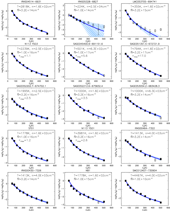
Figure 7: CO rotational diagrams for the Magellanic YSO targets (symbols as in Fig. 6), normalised to $N_{4}/g_{4}$. The thick blue line represents the best-fit model from $\chi^{2}$ minimisation; the shaded area represents models that fulfil a 1-$\sigma$ confidence interval. The best fit values for gas temperature $T$, molecular hydrogen volume density $n$ and CO column density parameter $\tilde{N}$ are listed in each panel; fit parameters are given in Table 6. A value for $\tau_{\rm max}$ is also provided if transitions become optically thick for the best fit model (see text for further details).

Table 6: Fit parameters to the observed CO rotational diagrams (CO (4$-$3) to CO (13$-12$)), using the non-LTE model grid by Neufeld (2012). The model parameters are gas temperature $T$ (in the approximate range 10 $-$ 5000 K, 0.05 logarithmic steps), molecular hydrogen volume density $n$ (160 $-$ $10^{12}$ cm^-3, 0.2 logarithmic steps) and CO column density parameter ${\tilde{N}}_{CO}$ ($10^{10}$ $-$ $10^{18}$ cm^-2 per km s^-1, 0.5 logarithmic steps). The best value is given for each parameter and the two limits provide the 1-$\sigma$ confidence interval (i.e. range for which $(\chi^{2}-\chi^{2}_{\rm min})$ $\leq$ 3.53). For IRAS05328$-$6827 the confidence interval includes the full parameter space. Values for maximum optical depth $\tau_{\rm max}$ and number of optically thick transitions $N(\tau>1)$, as well as $\chi^{2}$ values are also provided.

Source ID	$T$	$T_{\rm min}$	$T_{\rm max}$	$n$	$n_{\rm min}$	$n_{\rm max}$	$\tilde{N}$	$\tilde{N}_{\rm min}$	$\tilde{N}_{\rm max}$	$\tau_{\rm max}$	$N(\tau>1)$	$\chi^{2}$
	(K)			(m-3)			cm-2 per km s-2
LMC YSOs
IRAS 04514$-$6931	2818	1778	3162	160	160	630	3.2$\times$ 1014	1.0$\times$ 1010	1.0$\times$ 1016			8.6
IRAS 05328$-$6827	224			5000			1.0$\times$ 1014
LMC 053705$-$694741	355	178	501	160	160	4000	3.2$\times$ 1015	1.0$\times$ 1010	3.2$\times$ 1016			1.8
N113 YSO3	2239	1122	3162	250	160	2500	1.0$\times$ 1016	1.0$\times$ 1010	3.2$\times$ 1016	1.1	1	4.0
SAGE 045400.9$-$691151.6	501	355	891	630	160	16000	1.0$\times$ 1017	1.0$\times$ 1010	3.2$\times$ 1017	5.6	5	2.0
SAGE 051351.5$-$672721.9	794	501	1259	160	160	10000	3.2$\times$ 1017	1.0$\times$ 1010	3.2$\times$ 1017	17.0	6	3.3
SAGE 052202.7$-$674702.1	1995	1000	5012	250	160	4000	3.2$\times$ 1016	1.0$\times$ 1010	1.0$\times$ 1017	2.5	3	3.4
SAGE 052212.6$-$675832.4	1000	562	1413	160	160	4000	3.2$\times$ 1016	1.0$\times$ 1010	1.0$\times$ 1017	3.5	2	5.4
SAGE 053054.2$-$683428.3	1000	447	1995	6300	160	16000	3.2$\times$ 1014	1.0$\times$ 1010	3.2$\times$ 1017			4.0
ST 01	1778	1259	2818	160	160	1000	1.0$\times$ 1016	1.0$\times$ 1010	1.0$\times$ 1016	1.2	1	8.6
N113 YSO-1	3981	1778	5012	160	160	2500	3.2$\times$ 1016	1.0$\times$ 1010	3.2$\times$ 1016	2.6	3	1.9
SMC YSOs
IRAS 00464$-$7322	1413	794	5012	4000	160	6300	3.2$\times$ 1014	1.0$\times$ 1010	3.2$\times$ 1017			3.8
IRAS 00430$-$7326	1413	891	5012	4000	160	6300	3.2$\times$ 1014	1.0$\times$ 1010	3.2$\times$ 1017			2.5
N 81	1778	1413	2512	160	160	400	1.0$\times$ 1015	1.0$\times$ 1010	3.2$\times$ 1015			12.5
SMC 012407$-$730904	4467	2239	5012	400	160	1000	1.0$\times$ 1010	1.0$\times$ 1010	1.0$\times$ 1016			5.1

Neufeld (2012) showed that CO rotational diagrams can exhibit curvature, i.e. the rotational diagram changes monotonically with the upper level energy $E_{J}$ (mathematically $T_{\rm rot}\equiv-\left(k\,d\ln(N_{J}/g_{J})/dE_{J}\right)^{-1}$), for a single isothermal gas component if the gas is not thermalised. If the gas is sub-thermal, a positive curvature arises in the lower density regime, while for high but non-thermal densities a negative curvature results. In other words, a “break” in the rotational diagram does not necessarily imply multiple gas components.

Neufeld (2012) solved the equations of statistical equilibrium for CO gas, assuming a uniform density and temperature. Radiative transfer was treated using the escape probability method and a large velocity gradient in a single direction was assumed (for more details refer to Neufeld, 2012, and references therein). A pre-computed grid of solutions to the equations of statistical equilibrium for CO (David Neufeld, private communication) was fitted to the observed rotational diagrams, assuming a single uniform CO component. The grid parameters are gas temperature $T$ (in the approximate range 10 $-$ 5000 K, 0.05 logarithmic steps), molecular hydrogen volume density $n$ (160 $-$ $10^{12}$ cm^-3, 0.2 logarithmic steps) and CO column density parameter ${\tilde{N}}_{CO}$ ($10^{10}$ $-$ $10^{18}$ cm^-2 per km s^-1, 0.5 logarithmic steps; see Neufeld 2012 for a full description).

The rotational diagrams shown in Fig. 7 are normalised to $N_{4}/g_{4}$. For each object the best-fit model is shown in blue, and the dashed area indicates the range of models that correspond to a 1-$\sigma$ confidence interval for three free parameters ($\chi^{2}-\chi^{2}_{\rm min}$ $\leq$ 3.53). Fit parameters are given in Table 6; the maximum and minimum limits provide the 1-$\sigma$ confidence interval (note that often the best-fit value is at a limit of the grid). Values for $\chi^{2}$ and $\tau_{\rm max}$ (defined as the maximum value for the optical depth) are also provided for the best fit model (the latter only if transitions become optically thick).

Even though the parameters are not well constrained, a few facts are clear from the fits in Fig. 7 (we discuss only the thirteen objects with more than four transitions detected with good SNR). With the exception of two objects (SAGE 04500.9$-$691151.6 and SAGE 051351.5$-$672721.9) the best fit temperatures are high ($\sim$ 1000 $-$ 4500 K) and the molecular hydrogen densities are rather low ($\sim$ 160 $-$ 6300 cm^-3). As an independent check, we also compared our rotational diagrams to the grid of Radex models (van der Tak et al., 2007) used by Lee et al. (2016); similarly the parameters are poorly constrained but the $\chi^{2}$ fitting also favours high temperature, low density solutions. In fact, no model with density $n$  $>$ $\sim$  1.6 $\times 10^{4}$ cm^-3 is able to fit the data; at such low densities none of the energy levels are thermalised even at high temperature. Consequently, non-LTE models clearly favour sub-thermal excitation conditions.

The column density parameter is not constrained at all, but for seven out of thirteen sources the best solution sees one or more lower-$J$ transitions become optically thick; even in such cases there are optically thin models with slightly higher densities (but still $n$  $<$ $\sim$  1.6 $\times 10^{4}$ cm^-3) that provide acceptable fits. We note that no ¹³CO transitions were detected, and the upper limits do not place meaningful limits on the gas optical depth.

Purely in terms of $\chi^{2}$, the non-LTE fits are better than the LTE optically thin two-component fits (with fewer free parameters).

7.4 Properties of CO emitting gas: physical conditions and origin

As already pointed out, $L_{\rm{CO}}$ correlates strongly with a measure of YSO luminosity ($L_{\rm bol}$ or $L_{\rm TIR}$), for any YSO sample. There seems to be no correlation between parameters derived from the LTE analysis of the CO rotational diagrams and YSO properties, even taking into account uncertainties. The derived rotational temperatures are remarkably constant (variations are at most a factor two), while the YSO luminosity ($L_{\rm bol}$ or $L_{\rm TIR}$) changes by as much as five orders of magnitude across all samples. Therefore this suggests that while the amount of excited CO gas is related to the source luminosity the conditions of the excited gas are not.

However, the analysis of the CO rotational diagrams observed for Magellanic YSOs does not unambiguously pinpoint the gas conditions. A single high-temperature isothermal ($T$  $>$ $\sim$  1000 K) gas component can fit the observations, but the gas densities would be rather low ($n$  $<$ $\sim$  $10^{4}$ cm^-2), i.e. the hot gas would be very clearly subthermal. On the other hand, cold ($T$  $<$ $\sim$  200 K) LTE gas provides a good match for the observed CO intensities and ratios, but multiple components are required. Manoj et al. (2013) arrive at very similar conclusions, for their sample of low-luminosity ($L_{\rm bol}$  $<$ $\sim$  200 L_⊙) Galactic YSOs. They fitted CO rotational diagrams in the PACS range ($J$ $\geq$ 14), meaning that the temperatures derived are higher. Nevertheless, the ambiguity between the two regimes mentioned above is also seen. Manoj et al. (2013) argue that it is more difficult to conceive the existence of multiple LTE components with temperatures essentially insensitive to YSO luminosity. On the other hand, in the low-density regime, a large range in gas temperatures results in a narrow range in rotational temperatures: for a high luminosity YSO the CO gas may be hotter but the resulting CO emission is not significantly enhanced. This can also be seen in Fig. 7, where temperatures between 1000 and 5000 K result in models that are indistinguishable. Even though Manoj et al. (2013) favour the high temperature sub-thermal solutions, the fitted rotational diagrams alone cannot discriminate between the two sets of emitting gas conditions.

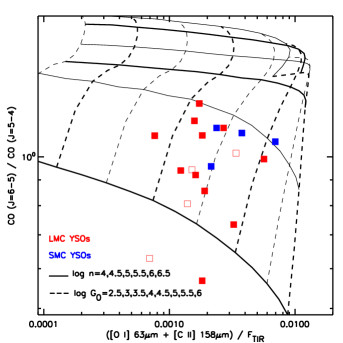
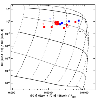
Figure 8: Observed atomic and CO emission compared to model predictions from the PDR Toolbox (Kaufman et al., 1999, 2006). Cloud density $n$ increases towards the top of the diagrams, and strength of the FUV radiation field $G_{0}$ increases towards the left. Symbols have the same meaning as in Fig. 5. The grid of PDR models represented in this figure covers a different range in parameter values (i.e. higher densities) than the grid in Fig. 4. Also note that $n$  $>$ $\sim$  $10^{4}$ cm^-3 is required when considering the ratio CO (6$-$5)/CO (5$-$4), while $n$  $>$ $\sim$  $10^{5}$ cm^-3 is appropriate for CO (13$-$12)/CO (5$-$4).

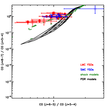
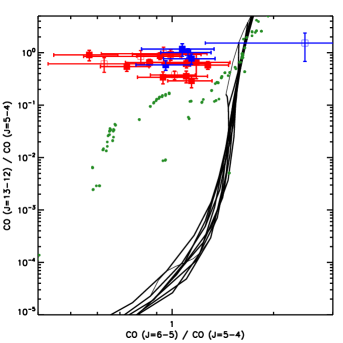
Figure 9: Observed CO emission ratios compared to model predictions from the PDR Toolbox (Kaufman et al., 1999, 2006) and shock models (Flower & Pineau des Forêts, 2015). PDR models (full lines) predict a very narrow range in CO line ratios, and a much steeper decrease (by several orders of magnitude) in fluxes for higher energy transitions, that is not observed. Green symbols show the ratios predicted by a selection of shock models (see text and also Lee et al., 2016). Shock heating is a more likely excitation mechanism for the observed CO emission.

The origin of the CO excitation can either be UV heating in PDRs or shock heating in molecular outflows. The constancy of the fitted rotational temperatures (over five orders of magnitude in luminosity, as shown in this work and Galactic samples – Manoj et al. 2013; Green et al. 2016; Yang et al. 2018), argues against UV photons as the main heating mechanism. To further explore this issue, we have compared CO emission line ratios to those predicted by the PDR models (Kaufman et al., 1999, 2006) used in Sect. 6.1.2 to analyse the [O i] and [C ii] emission. Figure 8 shows that the PDR conditions responsible for the atomic line emission (namely $n$  $<$ $\sim$  $10^{4}$ cm^-3, Fig. 4) are not consistent with the observed CO emission ratios for our sample: for the same photoelectric heating efficiency the required densities are higher ($n$  $>$ $\sim$  $10^{4}$ cm^-3). Therefore the same PDR gas is unlikely to be responsible for the atomic and CO emission (see also Stock et al., 2015, for two Galactic examples for which a similar conclusion was reached). Note that for 70% of the sources represented in Fig. 8, CO emission is optically thin for the transitions plotted (see Sect. 7.3.2). The diagram also suggests that the model density range that best reproduces the observed ratios progressively increases when higher-J CO transitions are considered: $n$  $>$ $\sim$  $10^{4}$ cm^-3 is required when considering the ratio CO (6$-$5)/CO (5$-$4), while $n$  $>$ $\sim$  $10^{5}$ cm^-3 is appropriate for CO (13$-$12)/CO (5$-$4). This indicates that a single PDR gas component cannot give rise to the observed CO emission across this energy range.

In Fig. 9 we further explore the behaviour of pairs of CO ratios. For CO gas excited in PDR conditions the predicted ratios occupy an extremely narrow range of values; for a given CO (6$-$5)/CO (5$-$4) ratio the PDR models predict a much steeper decrease (by five orders of magnitude) in CO (13$-$12) fluxes than what is actually observed (right panel). This is still the case even when only the CO cold component contribution (CO (8$-$7)/CO (5$-$4) ratio, left panel) is considered. We conclude that the CO emission observed towards Magellanic YSOs is very unlikely to be excited in PDRs, even when multiple gas components are considered. This is consistent with the analysis by Lee et al. (2016) who found that PDR heating cannot be responsible for the excitation of CO gas in the Magellanic SFR N 159W (see also Lee et al., 2019, for a similar analysis in the 30 Doradus region).

Figure 9 also shows the grid of shock models used by Lee et al. (2016, computed using the Paris$-$Durham shock code, ) for a range of representative conditions: pre-shock density $10^{4}$ $-$ $10^{6}$ cm^-3, unity magnetic field strength parameter (this parameter reflects the strength of magnetic field transverse to the shock propagation direction), and shock velocity 4 $-$ 20 km s^-1. This range of velocities is consistent with CO outflow velocities observed in the LMC (Fukui et al., 2015; Shimonishi et al., 2016). These shock models are for solar metallicity and do not include grain$-$grain interactions; none of these effects significantly impact CO line ratios over the J-range discussed here (see Appendix in Anderl et al. 2013 and Lee et al. 2016). Figure 9 (left) suggests that shock models are reasonably consistent with the observed CO emission ratios for Magellanic YSOs. However these models are still not able to fully reproduce the observed ratios over the whole J-range, i.e when higher-J transitions are included (Fig. 9 right). This suggests that if the CO emission originates from shocks, multiple gas components are required.

Meijerink et al. (2013) proposed that shock-heated gas both in SFRs and active galactic nuclei (AGN) can yield much larger $L_{\rm CO}/L_{\rm TIR}$ ratios than PDRs and XDRs (X-ray dominated regions). This is due to the fact that while PDRs and XDRs heat both the gas and the dust, shocks in typical conditions heat the dust less effectively, leading to larger ratios. Their models predict that a ratio $L_{\rm CO}/L_{\rm TIR}$  $>$ $\sim$  0.01% is the threshold diagnostic for shock heating. Most Galactic and all Magellanic objects in Fig. 5 exhibit ratios above this limit, suggesting that in massive YSO environments, CO is heated by shocks. Despite the very different spatial scales probed, both on SFR-wide scales and on the scales of individual massive YSOs shock-heated gas seems to be the origin of most CO emission.

High spectral resolution Herschel-HIFI observations of high-J CO and H₂O transitions in low-mass Galactic YSOs support the presence of at least three kinematically distinct gas components of different physical conditions within outflows (Kristensen et al., 2017, see their Fig. 10, and references therein): the cool component ( $<$ $\sim$  100 K, observed with SPIRE) originates from the entrained (i.e. swept-up) envelope gas, the warm component ($\sim$ 300 K, observed with PACS) comes from cavity shocks (gas directly interacting with the shocks in the walls of the outflow cavity) or from the disc wind, while the hot component ( $>$ $\sim$  600 K, observed with HIFI) emerges from distinct “spot shocks” near the base of the outflow or jet. The temperature of the ubiquitous warm $\sim$ 300 K component is the result from the change in the dominant cooling molecules from H₂ to CO, and the hot component arises in gas prior to the onset of H₂ formation. Both hotter components contribute to the excitation of H₂O emission (e.g., Mottram et al., 2014). As described in Sect. 7.2 the fact that the correlation between YSO luminosity and total CO luminosity extends from low-luminosity YSOs to massive YSOs supports a common origin for the observed CO emission across the mass range.

In summary, our analysis of the CO emission for massive YSOs in the Magellanic Clouds supports an origin in shocked gas. Multiple shock components are required to explain the observations (akin to what is observed for low-luminosity Galactic YSOs), suggesting the observed SPIRE emission is more likely to arise from LTE low-temperature gas (typically $T_{\rm cold}\sim 35$ K and $T_{\rm cool}\sim 132$ K for the Magellanic YSOs), rather than a single subthermal hot gas component.

7.5 Other lines in the SPIRE range

In this section we discuss atomic transitions detected in the SPIRE range. As already mentioned [N ii] emission traces the ionised gas that also contributes to the [C ii] emission, while [C i] emission traces regions where the gas is shielded enough so that carbon is found in a mixture of atomic C and CO.

7.5.1 [N ii] emission

Out of the nineteen sources observed with SPIRE, nine LMC and two SMC sources show [N ii] emission at 205 µm. We use the [N ii] emission to assess how much of the [C ii] emission originates from the ionised gas. Following the method proposed by Oberst et al. (2011), theoretical line intensity [C ii]/[N ii] ratios expected from ionised gas are used to estimate the ionised gas contribution to the total [C ii] emission. We calculate the fine structure level abundances of N⁺ and C⁺ as a function of electron density using theoretical collisional rates; a correction factor due to the ionic abundance fraction [(C⁺/C)/(N⁺/N)] = 1.26 is applied (determined using the MAPPINGS III photoionisation grid, Sutherland et al., 2013). Finally, we adopt a C/N ratio of 5.9 appropriate for H ii regions in the Galaxy and the Magellanic Clouds (Carlos Reyes et al., 2015, and references therein). For the typical low electron density $n_{\rm e}$ $\sim$ 100 cm^-3 that produces [C ii] emission (Cormier et al., 2015; Chevance et al., 2016), the theoretical ratios are ([C ii]/[N ii] 122 µm)_T $\sim$ 2.4 and ([C ii]/[N ii] 205 µm)_T $\sim$ 7.7. For the Magellanic sample, the observed ratios are ([C ii]/[N ii] 205 µm)_O > 20, calculated using the fluxes in Tables 9 and 10. The [C ii] PDR emission fraction is $1-($[C ii]/[N ii]$)_{\rm T}/($[C ii]/[N ii]$)_{\rm O}$; between 61% and 96% (median $\sim$ 82%) of the [C ii] emission originates from the PDR, rather than from low density ionised gas (individual fractions are listed in Table 9). For resolved star forming regions in the LMC and SMC, Cormier et al. (2015) estimated this contribution to be at least 75% (see also Lebouteiller et al. 2012; Chevance et al. 2016), while Jameson et al. (2018) estimated a contribution of $>$ $\sim$  95% for five SMC SFRs. Given the uncertainties, these estimates are reasonably consistent. Theoretical and observed [C ii]/[N ii] 122 µm  ratios are used to calculate the PDR gas fraction for the Galactic sample (Appendix E); a median of $\sim$ 60% of the [C ii] emission originates from the PDR gas component, broadly consistent with other estimates (Oberst et al., 2011; Bernard-Salas et al., 2012). Despite the large scatter for both Galactic and Magellanic samples, these fractions are also consistent with an increased contribution from the ionised gas component for higher metallicity environments (e.g., Cormier et al., 2019, and references therein).

7.5.2 [C i] emission

For five LMC objects and one SMC object we have detected [C i] emission at 370 and 609 µm; a further eight sources exhibit emission at 370 µm only. The ratio [C i]₃₇₀/[C i]₆₀₉ is sensitive to density and it can be used to infer the excitation temperature $T_{\rm ex}$ for optically thin LTE gas. Under such conditions the population levels follow a Boltzmann distribution (see also Spinoglio et al., 2012):

$$T_{\rm ex}=\Delta E\,\left[\ln\frac{N_{1}\,g_{2}}{N_{2}\,g_{1}}\right]^{-1},$$ (3)

where $\Delta E$ is the energy difference between the two levels (in K). Other quantities have their usual meanings; see Eq. 1 and 2 for their definition and the relation to observed line fluxes. For the Magellanic sample the [C i] line ratio varies in the range 1.2 $-$ 1.8, suggesting the emission is optically thin (e.g., Kramer et al., 2004). The inferred LTE excitation temperatures $T_{\rm ex}$ are in the narrow range 18 $-$ 24 K. If the C-emitting gas were not thermalised ($n\,\vbox{\hbox{$<$}\offinterlineskip\hbox{$\sim$}}\,10^{4}$ cm^-3, e.g., Tielens & Hollenbach, 1985), the observed ratios would favour higher temperature gas ($T_{\rm ex}$  $>$ $\sim$  30 K, see Fig. 9 in Pereira-Santaella et al. 2013).

The two sources with the lowest LTE temperature ($\sim$ 18 K) are SAGE 04500.9$-$691151.6 and SAGE 051351.5$-$672721.9; referring back to Sect. 7.3, these are the two sources for which the CO emission was closest to that predicted by a single isothermal gas component, and for which the two-component LTE fit predicted the lowest temperatures for the CO cool component (< 100 K).

We compared the ratios [C i]₃₇₀/[C i]₆₀₉ and [C i]₃₇₀/CO (CO measured over the SPIRE range) with the ratios predicted by shock models (Flower & Pineau des Forêts, 2015) – C-type shock: pre-shock density $n$ = $10^{3}$ $-$ $10^{6}$ cm^-3, shock velocity $v$ = 10 $-$ 40 km s^-1, magnetic field strength parameter $b$ = 1; J-type: $n$ = $10^{3}$ $-$ $10^{5}$ cm^-3, $v$ = 10 $-$ 35 km s^-1, $b$ = 0.1. For the [C i]₃₇₀/[C i]₆₀₉ ratio the predictions are $\vbox{\hbox{$>$}\offinterlineskip\hbox{$\sim$}}2$ and $\vbox{\hbox{$>$}\offinterlineskip\hbox{$\sim$}}3$ respectively for C- and J-type shocks. The [C i]₃₇₀/CO ratios are predicted to be $\vbox{\hbox{$<$}\offinterlineskip\hbox{$\sim$}}0.02$ and $\vbox{\hbox{$<$}\offinterlineskip\hbox{$\sim$}}0.036$, respectively. As already mentioned, for the Magellanic sample [C i]₃₇₀/[C i]₆₀₉ = 1.2$-$1.8 (for six sources), and [C i]₃₇₀/CO = 0.035$-$0.12 (for fourteen sources). The observed ratios are therefore not consistent with the [C i] emission originating in the same shocked gas that also is likely to produce the observed CO emission (see also Lee et al., 2016).

We also investigated whether the observed [C i] emission could originate from the PDR gas responsible for the [O i] and [C ii] emission, by looking at the [C i]₃₇₀/[C i]₆₀₉ ratio in conjunction with both the [O i]/[C ii] and the ([O i]+[C ii])/$F_{\rm TIR}$ ratios. We find that the [C i] emission is consistent with a low $G_{0}/n$ PDR regime, even if suggesting slightly lower $n$ and $G_{0}$ conditions than those derived from Fig. 4. As described in Röllig et al. (2007) the predicted intensities for [C i] are very model dependent, affecting the [C i] line ratio and the comparison with other atomic lines. Furthermore, [C i] emission may have a smaller filling factor and may trace different layers of the PDR compared to the [C ii] emission. Nevertheless, our analysis suggests that the [C i] emission in these sources originates from PDR gas.

8 Discussion

8.1 Line flux correlations

As already discussed in Sect. 6.1.2 there is a strong correlation between the [O i] and [C ii] emission, supporting their common origin in PDR gas. There is no correlation between total CO emission and these two atomic lines, consistent with a different origin for CO (likely shocked gas). We now discuss the relationships between the fluxes for other species in this study.

There is no correlation between H₂O emission at 179 µm and [O i] or [C ii] emission, supporting an origin in distinct gas components (see also Karska et al., 2018). Since H₂O emission is thought to originate from the warm and hot components ($T\vbox{\hbox{$>$}\offinterlineskip\hbox{$\sim$}}300$ K) of the outflow system in young stars (see discussion in Sect. 7.4) and [O i] or [C ii] emission originates from the PDR, this is to be expected. The CO emission measured over the SPIRE range originates from the distinct cool and cold component in the outflow system ($T_{\rm cool}$ $\sim$ 120 K and $T_{\rm cold}$ $\sim$ 40 K respectively); accordingly no correlation is found between H₂O and total CO emission.

OH emission is also thought to originate within the outflow (e.g., Wampfler et al., 2013), even though it has been difficult to consistently reconcile observed molecular emission with shock models (see discussion in Karska et al., 2018). We do not find any correlation between OH and H₂O emission; there is however a larger spread in the observed H₂O fluxes, compared to OH fluxes.

Most of the known H₂O maser sources exhibit H₂O emission in the PACS range; OH emission is detected towards one of two OH maser sources in the LMC.

8.2 Far-IR line cooling

In this section we discuss how the different atomic and molecular species contribute to the total line emission, an essential component of the cooling budget of the YSO environment.

8.2.1 Total emission line luminosities

For [O i], H₂O and OH we only have observations for a single line or doublet, and for CO we only observe over the SPIRE range, therefore we use correction factors to convert line fluxes to total luminosities; these are estimated from a variety of sources from the literature and described in previous sections. The corrections (i.e. multiplication factors) applied to the observed luminosities to obtain total luminosities are as follows: 1.09 for [O i] at 63 µm (adopted from Karska et al., 2018), 1.92 for CO observed in the SPIRE range (computed using the large dataset from Yang et al., 2018), 12.5 for H₂O observed at 179 µm, 4.17 for OH observed at 79 µm and finally 5.26 for OH observed at 84.4 µm only (estimated using data from Karska et al., 2013; Wampfler et al., 2013; Karska et al., 2018); no correction is needed to obtain [C ii] luminosities. We restrict our discussion of the gas cooling budget to the thirteen sources (nine LMC and four SMC) with good CO measurements across the SPIRE range. All these sources also have H₂O and OH measurements or 3-$\sigma$ upper limits. The total line luminosity $L_{\rm LIR}$ correlates moderately with the total IR luminosity $L_{\rm TIR}$ (Spearman’s parameters $\rho$ $\sim$ 0.7, $p$ $\sim$ 0.01); their ratio is $L_{\rm LIR}/L_{\rm TIR}$ $\sim$ 0.4% (range 0.2 $-$ 0.9%). Table 7 lists line luminosities for each species as fractions of $L_{\rm LIR}$, as well as $L_{\rm LIR}/L_{\rm TIR}$.

Table 7: Line luminosities as fractions of the total IR line luminosity $L_{\rm LIR}$ for [O i], [C ii], CO, and H₂O and OH when detected. The last column gives the ratio of total IR line luminosity to total IR luminosity $L_{\rm LIR}$/$L_{\rm TIR}$.

Source ID	$L_{\rm[OI]}$	$L_{\rm[CII]}$	$L_{\rm CO}$	$L_{\rm H_{2}O}$	$L_{\rm OH}$	$L_{\rm LIR}$
	($L_{\rm LIR}$)	($L_{\rm LIR}$)	($L_{\rm LIR}$)	($L_{\rm LIR}$)	($L_{\rm LIR}$)	($L_{\rm TIR}$)
LMC
IRAS04514$-$6931	0.43	0.22	0.26	0.06	0.03	0.003
N 113 YSO3	0.47	0.26	0.24	0.02	0.01	0.005
SAGE045400.9$-$691151.6	0.38	0.39	0.19	0.04	0.007	0.006
SAGE051351.5$-$672721.9	0.42	0.39	0.15			0.003
SAGE052202.7$-$674702.1	0.37	0.36	0.17			0.009
SAGE052212.6$-$675832.4	0.41	0.33	0.24			0.002
SAGE053054.2$-$683428.3	0.25	0.33	0.31			0.003
ST01	0.30	0.32	0.25			0.007
N 113 YSO1	0.36	0.25	0.36	0.03	0.004	0.005
SMC
IRAS00464$-$7322	0.26	0.32	0.28			0.009
IRAS00430$-$7326	0.51	0.30	0.09	0.05		0.003
N 81	0.75	0.10	0.05			0.009
SMC012407-730904	0.73	0.17	0.07			0.005

8.2.2 Contributions from [O i], [C ii] and CO to gas cooling

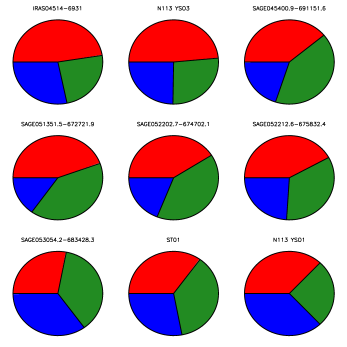
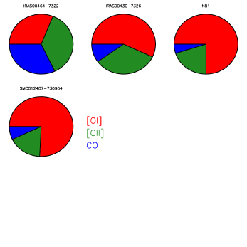
Figure 10: Fractions of gas cooling for LMC and SMC YSOs, for the main gas species discussed in this work: [O i] (red), [C ii] (green) and CO (blue). Note that the fractions displayed here are those from Table 7 renormalised to $L_{(\rm[OI]+[CII]+CO)}$ for sources with a contribution from H₂O and OH.

Figure 10 shows the relative contributions of [O i], [C ii] and CO that given their ubiquitous nature are expected to be the main contributors to far-IR line cooling in YSOs (e.g., Karska et al., 2013, 2014, 2018, and references therein). For the majority of the sources (8/13), the strongest line emission, and thus the main gas coolant, is [O i]; for four sources [C ii] is the main contributor, while for the last source CO and [O i] contribute in equal measure (with a smaller [C ii] contribution). Note that for many sources the [O i] and [C ii] contributions are very comparable. Median fractions normalised to their summed contributions are 42%, 34% and 24%, respectively for [O i], [C ii] and CO (source-to-source variations are significant). Luminosity fractions for [O i] and [C ii] are computed using line fluxes uncorrected for the extended emission contribution discussed in Sect. 6.1.1. This is to ensure that they can be compared to Galactic sources observed with ISO for which such corrections are unavailable. For completeness, if these corrections were applied to the Magellanic sources the fractions would become 46%, 23% and 31%, respectively for [O i], [C ii] and CO.

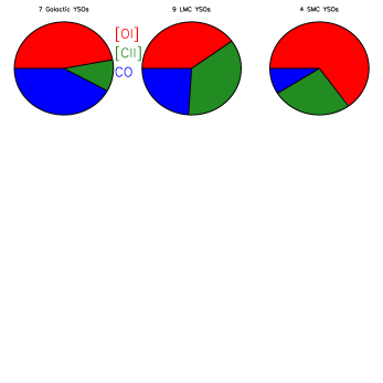
Figure 11: Median gas cooling contributions for the main gas species for the Galactic, LMC and SMC massive YSO samples (the number of objects in each sample is listed). The renormalised cooling fractions [O i]:[C ii]:CO are: 47:11:42 (Galaxy), 40:36:24 (LMC) and 65:26:9 (SMC).

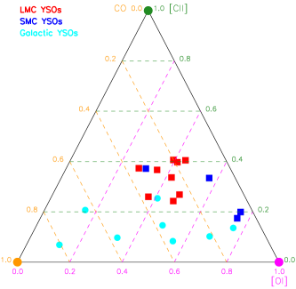
Figure 12: Ternary diagram showing the cooling fractions for the main gas species: [O i], [C ii] and CO. An object’s fractions should be read by following the colour-coded dashed lines ([O i] magenta, [C ii] green and CO orange) back to the relevant axes. Note that fractions displayed here are those from Table 7 renormalised to $L_{(\rm[OI]+[CII]+CO)}$.

We compared the luminosity fractions for massive Magellanic YSOs and Galactic massive YSOs observed with ISO LWS. As described in Sect. 5, we do not directly compare our Magellanic sample to the massive YSO sample described in Karska et al. (2014) due to the different spatial scales sampled. Furthermore, [C ii] emission is often saturated for those sources; when reliably detected, it accounts for between 10$-$25% of the total far-IR line luminosity. Individual gas cooling fractions for the Galactic comparison sources can be found in Fig. 19 and Table 12. The median contributions for the Galactic sample are 41%, 10% and 37%, respectively for [O i], [C ii] and CO. It is noticeable from Fig. 19 that for three out of seven sources CO is the main contributor to line emission while for the remaining four sources [O i] is the main contributor.

The renormalised median contributions for the LMC, SMC and Galactic massive YSO samples are shown in Fig. 11. The figure suggests that the contribution from [C ii] emission is reduced in the Galactic sample compared to the Magellanic sample. Furthermore, while in the Galaxy the median contributions of [O i] and CO are comparable, in the Magellanic sample [O i] emission is more dominant, particularly in the SMC. It is also noticeable that the CO relative contribution decreases from the Galaxy to the SMC, i.e. from higher to lower metallicity environments. Given that source-to-source variations are significant, the fractions for the individual sources from the different samples are shown collectively in the ternary diagram in Fig. 12. For the Magellanic sample, the [C ii] fractions are consistently between $\sim$ 20% and $\sim$40%. The [O i] fraction is larger than $\sim$ 30%, while the CO fraction is always less than 40%, in other words [O i] emission is dominant. For the Galactic sample, the [C ii] fraction is at most 25%, consistently lower than for the Magellanic sample. The range of the [O i] and CO contributions are comparable, but the diagram strongly suggests that there is more variation in terms of [O i]/CO ratio in the Galactic sample compared to the Magellanic sample.

We investigated in more detail the samples properties, to check for any trends and potential evolutionary effects. We constructed equivalent diagrams to that in Fig. 12, but separating sources with/without: silicate absorption, PAH and fine structure emission, and finally maser and radio emission (diagrams not shown). For more evolved sources in the UCH ii and later stages, radio emission is typically strong due to free$-$free emission in the ionised gas (e.g., Hoare, 2005). PAH emission and fine structure emission can also identify a more evolved source (with the caveat that the wider YSO environment can contaminate the Spitzer-IRS spectrum), while silicate absorption suggests a more embedded source (e.g., Seale et al., 2009; Woods et al., 2011). We found no statistically significant differences, either between the Galactic and Magellanic samples nor between samples with and without any of these indicators. Both the Galactic and Magellanic samples are made up of a very eclectic mix of sources, but there is no indication of any evolutionary effects.

Karska et al. (2014) found that for their sample of Galactic high-mass YSOs observed with PACS, line emission (and thus cooling) is dominated by CO and [O i], with a tendency for more evolved sources to have more significant [O i] contributions (as seen also for lower luminosity Galactic YSOs, Karska et al., 2018). In our analysis we find similarly large source-to-source variations but we find no evidence for any evolutionary trend. Nevertheless, while evolutionary effects cannot be completely ruled out, there seems to be a shift in cooling dominance from CO to [O i] from the Galaxy to the Magellanic Clouds (Figs. 11 and 12). Furthermore, the predominance of [O i] cooling seems to increase further for the SMC YSOs. Potentially, this could be a result of the lower CO gas-phase abundances at low metallicity, particularly in the SMC (e.g., Leroy et al., 2007).

We also analysed the behaviour of the [O i]/[C ii] and [O i]/CO ratios. Median [O i]/CO ratios are 1.2, 1.7 and 8 and [O i]/[C ii] ratios are 2.1, 1.1 and 2.7 respectively for Galactic, LMC and SMC samples. Kolmogorov$-$Smirnov (K$-$S) tests reveal that the three sets of [O i]/[C ii] measurements are statistically indistinguishable; for the [O i]/CO ratios the K$-$S tests between Magellanic and Galactic sources, and LMC and SMC YSOs reveal that these sets of measurements are distinct, with null hypothesis probabilities 0.08 and 0.04 respectively. We investigated the behaviour of these ratios as a function of several measurable quantities: $L_{\rm TIR}$ (or $L_{\rm bol}$ for the Galactic sources), CO₂ ice column density ($N({\rm CO_{2}})$, another potential indicator of a cooler environment; column densities are compiled from Gibb et al. 2004; Shimonishi et al. 2010; Oliveira et al. 2009, 2011; Seale et al. 2011), [O iii]$/L_{\rm TIR}$ or [O iii]$/L_{\rm bol}$ fraction, and finally mid-IR flux ratio ($F60/F100$ from IRAS photometry for Galactic sources and $F70/F100$ from Spitzer MIPS and Herschel PACS photometry for Magellanic sources, Tables 11 and 8 respectively). There are no significant correlations between the [O i]/[C ii] or [O i]/CO ratios with $L_{\rm TIR}$ or $L_{\rm bol}$, $N({\rm CO_{2}})$, and [O iii]$/L_{\rm TIR}$ or [O iii]$/L_{\rm bol}$. However Fig. 13 reveals that not only there seems to be a correlation between [O i]/CO ratio plotted against mid-IR flux ratio (albeit weak, Spearman $\rho$ = 0.53, $p$ = 0.034), the Galactic and Magellanic samples are different, as predicted by the K$-$S tests above. While being mindful of the small sample sizes, the mid-IR flux ratios are lower for Galactic sources; this suggests that the SED peaks at longer wavelengths, implying lower typical dust temperatures. The SMC sources tend to have higher ratios than the LMC sources, consistent with higher dust temperatures in the low-metallicity SMC environment (see Sect. 4, and e.g., van Loon et al., 2010a, b). Even though YSOs are generally associated with CO peaks (e.g., Sewiło et al., 2013), the observed CO emission is reduced for sources with higher dust temperature. This is consistent with the expectation that in general CO abundance is reduced and atomic species are more dominant in the less UV-shielded environments predominant at lower metallicity (e.g., Israel & Maloney, 2011).

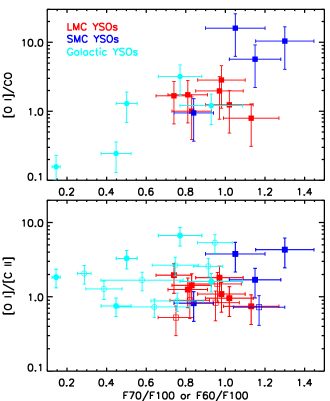
Figure 13: Cooling line ratios against mid-IR flux ratio: $F60/F100$ derived from IRAS fluxes for Galactic sources and $F70/F100$ derived from Spitzer MIPS and Herschel PACS fluxes for Magellanic sources. The uncertainties are dominated by the uncertainties resulting from the process to infer total line luminosities (Sect. 8.2.1). Filled symbols represent sources with CO measurements; sources shown with open symbols (lower panel) only have reliable [O i] and [C ii] measurements.

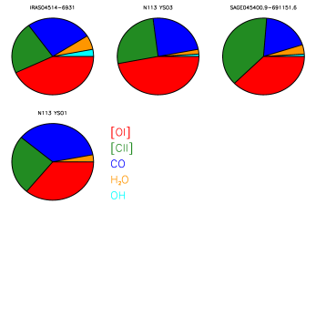
Figure 14: Cooling fractions for LMC YSOs, for those objects with H₂O (orange) and OH (cyan) detections. Note that for N 113-YSO1 the OH fraction is less than 1%. None of the SMC YSOs in our sample exhibit OH emission.

8.2.3 Contributions from H₂O and OH to gas cooling

For four out of thirteen sources both H₂O and OH measurements are available (in the LMC). For these sources H₂O and OH account for at most 6% and 3% of the total line cooling respectively, or at most 9% collectively (Fig. 14). If 3-$\sigma$ upper limits are considered, H₂O and OH could conservatively contribute up to 12% and 6% respectively. This indeed confirms that [O i], [C ii] and CO are definitively the main cooling agents ( $>$ $\sim$  90% of the total line cooling).

There is a clear trend of decreasing contribution of H₂O and OH cooling from low luminosity sources (Karska et al., 2018) to massive YSOs in the Galaxy (Karska et al., 2014). Our analysis suggests this trend extends to massive YSOs in the Magellanic Clouds. H₂O and OH molecules can be destroyed by numerous processes (see review by van Dishoeck, Herbst & Neufeld, 2013, and references therein), including photodissociation that would be more dominant in massive YSO environments. There could also be an evolutionary effect since H₂O emission is predominantly seen for evolved massive YSOs (van der Tak et al., 2013). However no such trend with evolutionary class is found in Karska et al. (2018).

9 Summary and Conclusions

We have presented Herschel PACS and SPIRE FTS spectroscopy of a sample of massive YSOs in the Magellanic Clouds. Our analysis focused on a variety of emission lines: [O i]  [O iii], [C ii], CO, H₂O and OH observed with PACS, and CO, [C i] and [N ii] observed with SPIRE. We have compared the properties of the Magellanic sample with those of a Galactic YSO sample observed with the ISO LWS; this is to ensure that the spatial scales probed by the two samples are in principle comparable. We summarise here our main findings:

• Bright atomic emission line morphology: [O i] and [C ii] emission is detected for all sources. By making use of the 25 PACS spaxels, we show that the emission exhibits a point source contribution superposed on more extended diffuse emission; we are able to successfully separate the YSO contribution. The morphology of the [O iii] emission is very varied: the YSO is detected for nine targets, while for four targets the emission at the YSO position is consistent with ambient contamination; for a further six targets no [O iii] emission is detected.

• Atomic emission line diagnostics and PDR emission: We find that [O i] and [C ii] emission (after removing the diffuse contribution (see above) and the ionised gas contribution to [C ii]) is tightly correlated, and it is also correlated with the total IR luminosity. The measured ratio [O i]/[C ii] is relatively low suggesting that shocks are not important contributors to [O i] emission. We conclude that both [O i] and [C ii] emission originate from the PDR associated with the massive YSOs. The line emission is also more dominant (with respect to the dust emission) in Magellanic YSOs when compared to the Galactic massive sample.

  The efficiency of photoelectric gas heating (inferred from the ratio ([O i]+[C ii])/$F_{\rm TIR}$) shows a large source-to-source scatter, however it is clearly higher for Magellanic compared to Galactic YSOs (medians respectively 0.25% and 0.1%). This can be understood as a consequence of the reduced grain charge in low metallicity environments. When compared to PDR models, our results are consistent with a lower $G_{0}/n$ ratio for the Magellanic sources, that can be interpreted as evidence of the changed properties in the low-metallicity ISM (porous and clumpy), even on the smaller spatial scales of individual YSOs.

  [N ii] emission at 205 µm is detected for nine LMC and two SMC YSOs. For these sources we are able to constrain the ionised gas contribution to the [C ii] emission. We conclude that most of the [C ii] emission originates from the PDR ($\sim$ 82% median). [C i] emission is detected at 370 and 609 µm for six sources. This emission originates from PDR gas, with a temperature of 18 $-$ 24 K for LTE gas or $\geq$ 30 K for non-LTE gas.

• Properties and origin of the CO emission: The observed CO emission is consistent with shock excitation. We analysed the CO rotational diagrams for fifteen sources. We find that these are broadly consistent with originating from either two low-temperature LTE gas components or a single isothermal (hot) low-density component. Based on the fact that CO ratios suggest the presence of multiple shock components, and on what is known from Galactic sources, the former seems the most likely scenario. The temperatures of the LTE components ($T_{\rm cold}$ $\sim$ 40 K and $T_{\rm cool}$ $\sim$ 120 K) are remarkably consistent across the luminosity range, and from Galactic to Magellanic environments.

• Additional molecular detections: H₂O emission is detected towards six LMC sources and tentatively towards one SMC source. OH emission is detected towards five sources, and absorption is detected towards two sources, all LMC YSOs. The emission is generally weak, as observed towards massive Galactic YSOs, signalling a very modest contribution to far-IR cooling (see below).

• YSO cooling budget: Our observations include the most prominent emission lines in YSO environments, that are thus the main contributors to the far-IR cooling of the YSO envelope, both in Galactic and Magellanic sources. We find that [O i] and [C ii] are the main contributors for Magellanic YSOs in contrast to Galactic YSOs for which CO and [O i] contribute by a similar amount, with a decreased [C ii] contribution. Furthermore, there seems to be a trend for a reduced fraction attributed to CO emission from the Galaxy $\rightarrow$ LMC $\rightarrow$ SMC, suggesting a link to metallicity. We find that the Magellanic YSOs not only have higher [O i]/CO ratios, they also have mid-IR fluxes consistent with higher dust temperatures. This is consistent with a reduction in CO emission in environments where the dust is warmer due to reduced UV-shielding.

Our analysis shows evidence for metallicity effects in the properties of the ISM in the near-environment of massive YSOs in the Magellanic Clouds. The interaction of the LMC and the SMC has potentially led to metallicity gradients in both galaxies (e.g., Fukui et al., 2017; Choudhury et al., 2018; Tsuge et al., 2019). It will be interesting to place our results in the context of these metal abundance variations, when such detailed large scale maps become available.

Appendix A Target SPITZER and HERSCHEL photometry

Table 8 lists the photometry for the Magellanic targets. Aperture photometry is performed for the Spitzer IRAC 3.6$-$8 µm and MIPS 24 and 70 µm bands (labelled I1$-$4 and M1$-$2): target centring, aperture radius and sky annulus radii are optimised for each target; a minimum 10% flux error is adopted. PSF band-merged catalogue photometry (Seale et al. 2014, see also Meixner et al. 2013) is used where available for the Herschel PACS (100 and 160 µm, P2$-$3) and SPIRE (250, 350 and 500 µm, S1$-$3) bands; for a single target (#4, N 81) ^∗ indicates that aperture photometry was used instead. We did perform aperture photometry for those sources for which only Herschel S1$-$S3 flux limits are available; however we do not consider those measurements reliable given the bright environmental emission and large beam size.

Table 8: Spitzer and Herschel photometry for the sample of Magellanic YSOs discussed here (flux densities in mJy). Photometric band identifications are as follows: I1$-$4: IRAC bands (3.6, 4.5, 5.8 and 8.0 µm); M1$-$2: MIPS bands (24 and 70 µm); P2$-$3: PACS bands (100 and 160 µm); S1$-$S3: SPIRE bands (250, 350 and 500 µm). We measure new aperture photometry for the I1$-$I4 and M1$-$M2 bands; a flux uncertainty of at least 10% is adopted for these measurements. We list catalogue (PSF) photometry for P2$-$P3 and S1$-$S3 from Seale et al. (2014) unless ^∗ indicates otherwise (aperture photometry is used for #4, N 81). Sources #7A, B are not resolved at all in any Herschel photometric bands, but two Spitzer sources are identified separated by $\sim 6$″; #7C is $\sim 20$″ from #7A, B and it is thus only resolved in PACS P2$-$3 (see Fig. 1, bottom). Sources #10, 11 and 12 are the three prominent YSOs in N 113 (see Fig. 1, top); they are spatially resolved in all Herschel bands (#10 and #12 are respectively $\sim 20$″ and $\sim 26$″ from #11), however only marginally so in the SPIRE photometric bands; thus it is not possible to extract meaningful individual fluxes in S2$-$3.

#	Source ID	I1	I2	I3	I4	M1	M2	P2	P3	S1	S2	S3
		3.6 µm	4.5 µm	5.8 µm	8 µm	24 µm	70 µm	100 µm	160 µm	250 µm	350 µm	500 µm
SMC YSOs
1	IRAS 00430$-$7326	34.8$\pm$3.5	70.1$\pm$7.0	123.4$\pm$12.3	144.3$\pm$14.4	1515$\pm$152	7798$\pm$780	6783$\pm$354	4467$\pm$305	1368$\pm$61	720$\pm$43	255$\pm$24
2	IRAS 00464$-$7322	3.9$\pm$0.4	8.9$\pm$0.9	15.7$\pm$1.6	21.1$\pm$2.1	120$\pm$12	1924$\pm$192	2279$\pm$127	2104$\pm$163	996$\pm$45	$\geq$234
3	S3MC 00541$-$7319	10.9$\pm$1.1	32.9$\pm$3.3	67.7$\pm$6.8	86.3$\pm$8.6	551$\pm$55	2591$\pm$259	2208$\pm$118	1475$\pm$113	$\geq$631	$\geq$469	$\geq$254
4	N 81	10.5$\pm$1.1	14.3$\pm$1.4	24.9$\pm$2.5	67.6$\pm$6.8	1296$\pm$130	9495$\pm$950	9049$\pm$905∗	7063$\pm$706∗	2742$\pm$274∗	1343$\pm$134∗	644$\pm$64∗
5	SMC 012407$-$73090 (N 88A)	35.5$\pm$3.5	72.3$\pm$7.2	138.8$\pm$13.9	429.9$\pm$43.0	7294$\pm$729	21720$\pm$2172	16390$\pm$875	8997$\pm$613	$\geq$2735	$\geq$1340	$\geq$706
LMC YSOs
6	IRAS 04514$-$6931	6.8$\pm$0.7	17.2$\pm$1.7	61.8$\pm$6.2	118.9$\pm$11.9	1696$\pm$170	13167$\pm$1317	17810$\pm$1164	12200$\pm$750	3484$\pm$218	$\geq$2445	1404$\pm$101
7A	SAGE 045400.2$-$691155.4	8.7$\pm$0.9	25.5$\pm$2.5	58.8$\pm$5.9	91.7$\pm$9.2	2617$\pm$262	$\leq$50597	11830$\pm$1141	21180$\pm$1342	10300$\pm$655	$\geq$3758	$\geq$3802
7B	SAGE 045400.9$-$691151.6	8.6$\pm$0.9	10.5$\pm$2.8	37.6$\pm$4.9	83.5$\pm$8.3
7C	SAGE 045403.0$-$691139.7	4.7$\pm$0.5	5.9$\pm$0.6	20.4$\pm$2.0	45.4$\pm$4.5	1456$\pm$155	$\leq$48865	8862$\pm$1085	11720$\pm$841
8	IRAS 05011$-$6815	1.0$\pm$0.2	1.7$\pm$0.3	3.1$\pm$0.4	5.4$\pm$0.7	445$\pm$44	4762$\pm$476	5026$\pm$333	3994$\pm$258	$\geq$1756	1212$\pm$65	687$\pm$50
9	SAGE 051024.1$-$701406.5	8.8$\pm$0.9	31.2$\pm$3.1	73.4$\pm$7.3	116.0$\pm$11.6	588$\pm$59	2470$\pm$247	3279$\pm$220	3108$\pm$204	1770$\pm$108	940$\pm$49	372$\pm$28
10	N 113 YSO-1	14.6$\pm$1.5	21.6$\pm$2.2	85.7$\pm$8.6	234.0$\pm$23.4	5130$\pm$513	49959$\pm$4996	60100$\pm$4056	54880$\pm$3345	20540$\pm$1284	$\geq$3074	$\geq$5855
11	N 113 YSO-4	17.5$\pm$1.7	27.6$\pm$2.8	84.2$\pm$8.4	207.2$\pm$20.7	4797$\pm$480	17469$\pm$1747	18200$\pm$1502	19820$\pm$1274	5705$\pm$379
12	N 113 YSO-3	17.3$\pm$1.7	25.7$\pm$2.6	82.3$\pm$8.2	226.2$\pm$22.6	4809$\pm$481	43832$\pm$4383	45210$\pm$2989	30460$\pm$1871	11480$\pm$714
13	SAGE 051351.5$-$672721.9	11.6$\pm$1.2	17.6$\pm$1.8	72.6$\pm$7.3	189.6$\pm$19.0	3870$\pm$387	20677$\pm$2068	21060$\pm$1388	15700$\pm$961	6405$\pm$392	2721$\pm$147	985$\pm$77
14	SAGE 052202.7$-$674702.1	4.3$\pm$0.4	3.9$\pm$0.4	19.2$\pm$1.9	49.6$\pm$5.0	869$\pm$87	$\leq$8437	7020$\pm$474	7201$\pm$453	4015$\pm$246	1914$\pm$107	969$\pm$76
15	SAGE 052212.6$-$675832.4	41.7$\pm$4.2	95.1$\pm$9.5	231.0$\pm$23.1	377.3$\pm$37.8	7935$\pm$794	43135$\pm$4314	53050$\pm$3488	31420$\pm$1924	8222$\pm$524	3354$\pm$216	$\geq$4127
16	SAGE 052350.0$-$675719.6	2.7$\pm$0.3	4.7$\pm$0.5	18.6$\pm$1.9	52.0$\pm$5.2	1400$\pm$140	10694$\pm$1070	13100$\pm$860	9640$\pm$598	3921$\pm$241	1897$\pm$106	$\geq$ 821
17	SAGE 053054.2$-$683428.3	31.6$\pm$3.2	70.8$\pm$7.1	142.4$\pm$14.2	192.9$\pm$19.4	1731$\pm$173	14416$\pm$1442	12780$\pm$853	10180$\pm$636	$\geq$3551	$\geq$1823	$\geq$1436
18	IRAS 05328$-$6827	61.1$\pm$6.1	101.9$\pm$10.2	168.0$\pm$16.8	185.8$\pm$18.6	551$\pm$55	$\leq$4794	2556$\pm$210	3581$\pm$253	$\geq$1884	$\geq$1133	$\geq$ 779
19	LMC 053705$-$694741	2.0$\pm$0.2	1.4$\pm$0.1	9.9$\pm$1.0	25.0$\pm$2.5	$\geq$71.5	$\leq$4351	1428$\pm$180	1865$\pm$197	835$\pm$89		$\geq$1041
20	ST 01	18.4$\pm$1.8	35.5$\pm$3.6	83.3$\pm$8.3	137.5$\pm$13.8	888$\pm$89	9129$\pm$913	8967$\pm$602	7793$\pm$492	$\geq$4134	$\geq$1861	$\geq$1315

Appendix B Selected SED fit examples

Figure 15 shows examples of the two component modified blackbody fits to the SEDs of Magellanic YSOs, as described in Sect. 4. The fit parameters for individual objects are tabulated in Table 4. The integrated luminosity $L($ > 10 µm) is adopted as the object’s total IR luminosity $L_{\rm TIR}$. Example spectra for the same two sources are shown in Fig. 16.

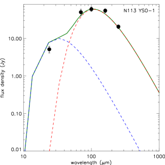
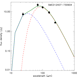
Figure 15: Examples of two component modified blackbody SED fits for N 113 YSO-1 (in the LMC) and SMC 012407$-$730904 (N 88A). The total fit (green line) is shown, as well as the two temperature components: the temperature of the warmer components (blue dashed line) is not well constrained; the cooler component (red line) has temperature of $\sim$ 34 K and $\sim$ 38 K respectively for these two examples.

Appendix C Selected example spectra

Figure 16 shows examples of the PACS and SPIRE spectra for an LMC and an SMC YSO respectively. They are typical of our sample for [O i], [O iii] and [C ii]; for CO they exemplify the highest and the lowest SNR achieved. The SPIRE spectra are representative of those sources with SNR $\geq$ 5 for which the analysis of the rotational diagram was performed. This SNR limit was chosen somewhat empirically; as discussed in Sect. 7.1, for lower SNR the centroid line positions vary widely and line identifications become unreliable. It is consistent with limits set in other works (Lee et al., 2016). Note that for the SMC source SMC 012407$-$730904, emission for [C i] at 609 µm and [N ii] at 205 µm are not detected.

In Figs. 17 and 18 we show H₂O and OH spectra for those sources for which the transitions are detected. N 113-YSO3 is the only source for which both the 179.5 and 108 µm transitions were detected; the detection of H₂O at 108 µm for IRAS 00430$-$7326 is very tentative. For the OH doublet at 84 µm the bluest component is detected in emission for two sources. For OH at 79.1 µm emission is detected for three sources, for N 113-YSO1 only the blue component is detected and for SAGE 052212.6$-$675832.4 and SAGE 052350.0$-$675719.6 weak absorption is detected. No OH transitions are detected towards any SMC source. Line fluxes are tabulated in the next section.

Figure 16: PACS and SPIRE spectra for N 113 YSO-1 (in the LMC) and SMC 012407$-$730904 (N 88A).

Figure 17: H₂O detections for Magellanic YSOs. Note that N 113 YSO-3 is the only source for which both the 179.5 and 108 µm transitions were detected. For the SMC source IRAS 00430$-$7326 there is a tentative detection at 108 µm only. The vertical dashed line represent the galaxies systemic velocity.

Figure 18: OH detections for Magellanic YSOs. Most sources shown exhibit OH emission for at least one doublet component; for SAGE 052212.6$-$675832.4 and SAGE 052350.0$-$675719.6 weak absorption is detected. The redmost doublet component is displayed at the galaxies systemic velocity.

Appendix D Line fluxes for Magellanic YSOs

In this section we present measured line fluxes and 3-$\sigma$ upper limits for individual Magellanic YSOs. These are shown in Tables 9 and 10 respectively for lines observed with PACS and SPIRE FTS.

Table 9: Measured fluxes for Magellanic YSOs for lines in the PACS range ($\times 10^{-18}$ W m^-2). Upper limits are given at 3-$\sigma$. For [O i], [C ii] and [O iii] both measured fluxes and fluxes corrected for the extended environmental emission (Sect 6.1.1) are given; for [O iii] if the latter is not listed the emission is considered to be mostly ambient to the YSO wider environment. The fraction of [C ii] emission that originates from the PDR gas is also given (see Sect 7.5.1). Sources #7A and B are not resolved at PACS wavelengths.

#	SourceID	[O i] 63 µm		[C ii] 158 µm			[O iii] 88 µm		CO	H2O		OH
		Measured	Corrected	Measured	Corrected	PDR	Measured	Corrected	186 µm	108 µm	179.5 µm	79.11 µm	79.18 µm	84.4 µm	84.6 µm
SMC YSOs
1	IRAS 00430$-$7326	1010.0$\pm$ 6.8	900.0$\pm$ 6.8	648.1$\pm$ 6.5	471.0$\pm$ 6.7	0.96	116.8$\pm$ 3.0	116.7$\pm$ 3.0	$\leq$16.8	11.3$\pm$ 3.3	$\leq$16.8	$\leq$19.9	$\leq$19.9
2	IRAS 00464$-$7322	228.8$\pm$ 4.1	210.0$\pm$ 4.1	303.0$\pm$ 3.9	150.0$\pm$ 4.0	0.74					$\leq$ 7.4	$\leq$11.0	$\leq$11.0
3	S3MC 00541$-$7319	115.9$\pm$ 5.1	115.0$\pm$ 5.0	173.9$\pm$ 3.4	121.0$\pm$ 3.8	1.00	$\leq$ 17.3		16.9$\pm$ 3.1	$\leq$11.8	$\leq$ 8.1	$\leq$11.1	$\leq$11.1	$\leq$10.3	$\leq$10.3
4	N 81	2955.8$\pm$18.4	2670.0$\pm$18.4	848.3$\pm$ 6.8	680.0$\pm$ 6.8	1.00	4771.0$\pm$12.8	4290.0$\pm$ 8.8	$\leq$11.0	$\leq$20.8	$\leq$14.1			$\leq$10.7	$\leq$10.7
5	SMC 012407$-$730904	5729.6$\pm$16.6	5400.0$\pm$16.6	1442.4$\pm$11.6	1160.0$\pm$11.8	1.00	1671.9$\pm$ 7.0	1580.0$\pm$ 7.0	18.4$\pm$ 4.0	$\leq$24.4	$\leq$14.0	$\leq$21.0	$\leq$21.0	$\leq$13.5	$\leq$13.5
LMC YSOs
6	IRAS 04514-6931	1118.1$\pm$ 6.2	1100.0$\pm$16.0	621.7$\pm$ 5.1	500.0$\pm$ 5.0	1.00	$\leq$ 19.4		$\leq$25.2	$\leq$17.7	14.0$\pm$ 2.0			16.8$\pm$ 3.8	$\leq$13.0
7A	SAGE 045400.2$-$691155.4	3757.4$\pm$26.4	3000.0$\pm$26.9	3082.3$\pm$19.8	1850.0$\pm$21.3	0.74	5061.7$\pm$17.1		$\leq$32.5	$\leq$32.8	$\leq$14.0	4.8$\pm$ 2.9	19.1$\pm$ 3.7	$\leq$24.7	$\leq$24.7
7B	SAGE 045400.9$-$691151.6
7C	SAGE 045403.0$-$691139.7	1557$\pm$12.9	800$\pm$13.9	2890$\pm$24.9	1660$\pm$26.1	0.72	4340$\pm$24.6		$\leq$35.3	$\leq$53.2	44.7$\pm$11.9	$\leq$27.6	$\leq$27.6	$\leq$24.1	$\leq$24.1
8	IRAS 05011$-$6815	91.4$\pm$16.2	90.0$\pm$ 0.2	119.1$\pm$ 8.1	94.0$\pm$ 8.9	1.00	$\leq$ 21.8		$\leq$20.9	$\leq$34.0	23.2$\pm$ 5.5	$\leq$18.4	$\leq$18.4	$\leq$14.5	$\leq$14.5
9	SAGE 051024.1$-$701406.5	140.1$\pm$ 9.1	140.0$\pm$ 9.1	289.4$\pm$ 7.6	217.0$\pm$18.0	1.00	$\leq$ 24.9		12.9$\pm$ 5.7	$\leq$19.0	$\leq$22.2	$\leq$16.8	$\leq$16.8	$\leq$22.1	$\leq$22.1
10	N 113 YSO1	5218.3$\pm$22.2	3500.0$\pm$23.3	3974.4$\pm$22.3	1990.0$\pm$24.8	0.78	2635.8$\pm$10.1	2310.0$\pm$10.0	121.4$\pm$ 7.4	$\leq$44.1	39.6$\pm$15.7	13.9$\pm$ 3.7	$\leq$20.1	$\leq$32.8	$\leq$32.8
11	N 113 YSO4	5186.2$\pm$27.6	3470.0$\pm$28.4	3777.5$\pm$19.8	1796.0$\pm$22.7		6459.7$\pm$18.0	6130.0$\pm$18.0	26.4$\pm$ 9.7	$\leq$44.6	16.1$\pm$ 2.8	22.0$\pm$ 4.3	5.8$\pm$ 3.3	$\leq$20.9	$\leq$20.9
12	N 113 YSO3	6192.8$\pm$26.8	4333.0$\pm$18.7	3723.1$\pm$25.7	1700.0$\pm$28.0	0.91	208.0$\pm$ 5.9		45.9$\pm$ 5.1	28.0$\pm$ 8.5	29.2$\pm$ 5.6	6.5$\pm$ 6.3	19.6$\pm$ 5.3	37.7$\pm$ 5.4	$\leq$16.3
13	SAGE 051351.5$-$672721.9	1701.6$\pm$ 7.5	1530.0$\pm$ 7.5	1700.2$\pm$13.5	1180.0$\pm$14.0	0.91	164.6$\pm$ 3.9		22.0$\pm$ 6.2	$\leq$27.9	$\leq$16.3	$\leq$15.4	$\leq$15.4
14	SAGE 052202.7$-$674702.1	1173.1$\pm$11.9	1050.0$\pm$11.8	1226.1$\pm$ 9.4	1000.0$\pm$ 9.5	0.86	$\leq$ 38.3		$\leq$25.8	$\leq$32.9	$\leq$17.5	$\leq$25.9	$\leq$25.9	$\leq$22.2	$\leq$22.2
15	SAGE 052212.6$-$675832.4	3314.4$\pm$16.2	2330.0$\pm$11.2	2881.4$\pm$17.3	800.0$\pm$ 5.0	0.81	8227.4$\pm$29.0		$\leq$29.5	$\leq$34.6	$\leq$18.2	$-$10.8$\pm$ 4.0	$-$30.3$\pm$ 0.7	$\leq$38.5	$\leq$38.5
16	SAGE 052350.0$-$675719.6	588.7$\pm$ 8.4	522.0$\pm$ 8.4	714.4$\pm$ 6.3	500.0$\pm$ 6.4	1.00	17.3$\pm$ 5.0	17.3$\pm$ 5.0	$\leq$18.1	$\leq$25.3	$\leq$20.3	$-$6.4$\pm$ 1.5	$-$5.3$\pm$ 1.0	$\leq$22.1	$\leq$22.1
17	SAGE 053054.2$-$683428.3	598.3$\pm$ 6.7	539.0$\pm$ 6.7	873.9$\pm$ 9.3	610.0$\pm$ 9.6	0.76	1712.1$\pm$ 8.0	78.0$\pm$13.0	$\leq$15.1	$\leq$34.1	$\leq$22.8	$\leq$12.2	$\leq$12.2
18	IRAS 05328$-$6827	108.3$\pm$ 9.1	100.0$\pm$ 9.0	539.0$\pm$ 7.7	160.0$\pm$ 9.4	0.81	13.9$\pm$ 3.7	14.0$\pm$ 3.7	13.1$\pm$ 5.6	$\leq$32.8	$\leq$27.6	$\leq$21.2	$\leq$21.2	$\leq$20.9	$\leq$20.9
19	LMC 053705$-$694741	80.6$\pm$ 3.9	25.0$\pm$ 4.0	615.8$\pm$ 6.1	92.0$\pm$ 8.9	0.62	36.7$\pm$ 4.7	37.0$\pm$ 4.7	$\leq$23.2	$\leq$30.2	$\leq$24.2	$\leq$12.9	$\leq$12.9
20	ST 01	1000.5$\pm$ 9.9	900.0$\pm$22.4	1137.0$\pm$ 7.5	790.0$\pm$ 8.3	1.00	$\leq$ 27.9		$\leq$25.1	$\leq$19.6	$\leq$26.4	$\leq$17.2	$\leq$17.2	$\leq$16.9	$\leq$16.9

Table 10: Measured fluxes for Magellanic YSOs for lines in the SPIRE FTS range ($\times 10^{-18}$ W m^-2). Upper limits are given at 3-$\sigma$. Sources #7A, B and C are not resolved in these SPIRE observations; source #11 has no SPIRE spectrum. For the sources marked $*$, the SNR ratio is not sufficient for the analysis of the CO rotational diagram.

		CO										[C i]		[N ii]
		4$-$3	5$-$4	6$-$5	7$-$6	8$-$7	9$-$8	10$-$9	11$-$10	12$-$11	13$-$12	370 µm	609 µm	205 µm
SMC YSOs
1	IRAS 00430$-$7326	5.4$\pm$ 1.0	12.2$\pm$ 1.0	11.7$\pm$ 1.0	10.0$\pm$ 1.0	12.5$\pm$ 1.0	11.1$\pm$ 0.9	10.6$\pm$ 0.9	10.5$\pm$ 0.9	9.2$\pm$ 0.9	7.1$\pm$ 0.9	5.1$\pm$ 1.0	$\leq$ 3.1	3.4$\pm$ 0.9
2	IRAS 00464$-$7322	7.8$\pm$ 1.2	15.8$\pm$ 1.2	18.1$\pm$ 1.2	17.4$\pm$ 1.2	15.8$\pm$ 1.2	19.6$\pm$ 1.9	10.8$\pm$ 1.9	13.1$\pm$ 1.9	6.3$\pm$ 1.9	12.2$\pm$ 1.9	12.1$\pm$ 1.2	7.7$\pm$ 1.2	10.3$\pm$ 1.9
3	S3MC 00541$-$7319∗	$\leq$ 4.4	3.4$\pm$ 1.5	8.3$\pm$ 1.5	6.0$\pm$ 1.5	9.8$\pm$ 1.5	5.6$\pm$ 1.6	1.5$\pm$ 1.6	2.8$\pm$ 1.6	$\leq$ 4.7	5.1$\pm$ 1.6	$\leq$ 4.5	$\leq$ 4.4	$\leq$ 4.7
4	N 81	13.5$\pm$ 1.3	9.1$\pm$ 1.3	9.7$\pm$ 1.3	11.9$\pm$ 1.4	8.2$\pm$ 1.3	13.2$\pm$ 1.9	11.2$\pm$ 1.9	10.2$\pm$ 1.9	6.4$\pm$ 1.9	10.6$\pm$ 1.9	$\leq$ 4.1	$\leq$ 4.0	$\leq$ 5.7
5	SMC 012407$-$730904	24.6$\pm$ 1.8	25.8$\pm$ 1.8	28.8$\pm$ 1.8	30.9$\pm$ 1.8	33.8$\pm$ 1.8	42.4$\pm$ 2.4	39.3$\pm$ 2.4	27.4$\pm$ 2.4	32.2$\pm$ 2.4	26.0$\pm$ 2.4	10.0$\pm$ 1.8	$\leq$ 5.5	$\leq$ 7.3
LMC YSOs
6	IRAS 04514$-$6931	38.3$\pm$ 1.7	37.1$\pm$ 1.7	40.9$\pm$ 1.7	38.8$\pm$ 1.7	33.2$\pm$ 1.7	44.2$\pm$ 2.2	41.1$\pm$ 2.2	45.1$\pm$ 2.2	34.9$\pm$ 2.2	23.0$\pm$ 2.2	19.4$\pm$ 1.7	$\leq$ 5.1	$\leq$ 6.5
7A	SAGE 045400.2$-$691155.4	109.7$\pm$ 7.0	180.5$\pm$ 6.9	206.1$\pm$ 6.9	234.9$\pm$ 7.1	213.0$\pm$ 6.9	214.5$\pm$11.1	152.6$\pm$11.1	95.2$\pm$11.1	74.7$\pm$11.1	52.4$\pm$11.2	71.2$\pm$ 7.1	63.2$\pm$ 7.0	102.7$\pm$10.9
7B	SAGE 045400.9$-$691151.6
7C	SAGE 045403.0$-$691139.7
8	IRAS 05011$-$6815∗	19.2$\pm$ 3.8	24.7$\pm$ 3.7	15.5$\pm$ 3.7	12.3$\pm$ 3.8	10.2$\pm$ 3.7	10.2$\pm$ 3.5	6.7$\pm$ 3.5	2.8$\pm$ 3.5	12.2$\pm$ 3.5	15.1$\pm$ 3.5	$\leq$11.4	$\leq$11.4	$\leq$10.6
9	SAGE 051024.1$-$701406.5∗	20.9$\pm$ 3.4	15.6$\pm$ 3.4	14.7$\pm$ 3.4	15.3$\pm$ 3.4	10.2$\pm$ 3.4	9.6$\pm$ 3.1	8.2$\pm$ 3.1	4.2$\pm$ 3.1	1.7$\pm$ 3.1	14.9$\pm$ 3.1	$\leq$10.2	$\leq$10.3	$\leq$ 9.4
10	N 113 YSO1	180.8$\pm$ 8.2	307.0$\pm$ 8.1	282.5$\pm$ 8.1	338.7$\pm$ 8.2	317.8$\pm$ 8.1	315.9$\pm$10.1	323.0$\pm$10.1	317.3$\pm$10.1	289.5$\pm$10.1	266.8$\pm$10.2	124.0$\pm$ 8.2	65.8$\pm$ 8.1	112.1$\pm$10.1
11	N 113 YSO4
12	N 113 YSO3	152.8$\pm$ 7.7	220.7$\pm$ 7.6	188.9$\pm$ 7.6	223.9$\pm$ 7.7	224.2$\pm$ 7.6	183.9$\pm$ 8.9	141.8$\pm$ 8.9	155.4$\pm$ 8.9	140.1$\pm$ 8.9	142.8$\pm$ 8.9	75.9$\pm$ 7.7	42.9$\pm$ 7.6	43.4$\pm$ 8.8
13	SAGE 051351.5$-$672721.9	20.9$\pm$ 1.4	31.3$\pm$ 1.4	39.9$\pm$ 1.4	47.7$\pm$ 1.4	44.6$\pm$ 1.4	50.4$\pm$ 1.5	38.2$\pm$ 1.5	28.4$\pm$ 1.5	19.1$\pm$ 1.5	18.1$\pm$ 1.5	11.8$\pm$ 1.4	10.3$\pm$ 1.4	19.5$\pm$ 1.5
14	SAGE 052202.7$-$674702.1	21.4$\pm$ 3.9	29.8$\pm$ 3.8	29.5$\pm$ 3.8	38.6$\pm$ 3.9	47.1$\pm$ 3.8	34.9$\pm$ 3.5	23.8$\pm$ 3.5	26.8$\pm$ 3.5	24.8$\pm$ 3.5	27.6$\pm$ 3.5	28.2$\pm$ 3.9	$\leq$11.7	22.4$\pm$ 3.5
15	SAGE 052212.6$-$675832.4	120.6$\pm$ 7.3	153.4$\pm$ 7.2	169.0$\pm$ 7.2	152.6$\pm$ 7.4	119.8$\pm$ 7.2	83.2$\pm$11.0	120.7$\pm$11.0	63.6$\pm$11.0	42.6$\pm$11.0	54.6$\pm$11.1	98.9$\pm$ 7.4	$\leq$22.1	69.5$\pm$10.9
16	SAGE 052350.0$-$675719.6∗	$\leq$20.3	36.6$\pm$ 6.7	29.5$\pm$ 6.7	28.1$\pm$ 6.8	18.8$\pm$ 6.7	21.1$\pm$ 5.7	$\leq$17.2	21.0$\pm$ 5.7	18.9$\pm$ 5.7	31.1$\pm$ 5.7	$\leq$20.4	$\leq$20.3	$\leq$17.2
17	SAGE 053054.2$-$683428.3	21.0$\pm$ 2.9	56.4$\pm$ 2.9	53.0$\pm$ 2.9	53.6$\pm$ 2.9	52.4$\pm$ 2.9	52.0$\pm$ 4.0	44.5$\pm$ 4.0	38.5$\pm$ 4.0	34.6$\pm$ 4.0	19.2$\pm$ 4.0	27.5$\pm$ 2.9	15.5$\pm$ 2.9	26.8$\pm$ 4.0
18	IRAS 05328$-$6827	12.3$\pm$ 4.5	26.6$\pm$ 4.4	31.4$\pm$ 4.4	24.2$\pm$ 4.5	25.0$\pm$ 4.4	19.8$\pm$ 8.0	33.8$\pm$ 8.0	17.0$\pm$ 8.0	3.2$\pm$ 8.0	17.4$\pm$ 8.1	23.9$\pm$ 4.5	$\leq$13.4	74.3$\pm$ 8.0
19	LMC 053705$-$694741	50.2$\pm$ 3.7	45.1$\pm$ 3.6	25.6$\pm$ 3.6	17.0$\pm$ 3.7	20.2$\pm$ 3.6	13.0$\pm$ 6.5	15.0$\pm$ 6.5	8.4$\pm$ 6.5	19.0$\pm$ 6.5	40.8$\pm$ 6.5	22.4$\pm$ 3.7	$\leq$11.0	30.6$\pm$ 6.5
20	ST 01	47.6$\pm$ 3.6	71.3$\pm$ 3.6	52.3$\pm$ 3.6	54.9$\pm$ 3.6	38.2$\pm$ 3.6	43.0$\pm$ 4.5	34.8$\pm$ 4.5	33.3$\pm$ 4.5	41.5$\pm$ 4.5	38.7$\pm$ 4.5	32.4$\pm$ 3.6	$\leq$10.9	$\leq$13.6

Appendix E Galactic massive YSO sample observed with ISO

Table 11: Galactic massive YSOs observed with ISO and used as a Galaxy comparison sample. TDT number is the unique identifier for ISO observations. References for source bolometric luminosities and distances are as follows: 1: van der Tak et al. (2013); 2: Stock et al. (2015); 3: Guzmán et al. (2012); 4: Lumsden et al. (2012); 5: de Wit et al. (2009); 6: Navarete et al. (2015); 7: Boley et al. (2013) 8: de Wit et al. (2011). The three sources that do not show [O i] in emission at 63 µm (source ID between parentheses, “a” and “u” in the [O i] notes column respectively for line in absorption and undetected) are listed for completeness but are not included in further analysis. $F60$ and $F100$ are fluxes from IRAS catalogues (uncertainties < 20%). For the sources used in the cooling budget discussion in Sect 8.2.2 additional properties are provided in the last column: ice absorption, 9: Gibb et al. (2004); H₂O maser emission, 10: Palagi et al. (1993); radio emission, 11: Wilson et al. (2003), 12: Wendker, Higgs & Landecker (1991), 13: Momose et al. (2001).

Source ID	RA (J2000)	Dec	TDT #	$L_{\rm bol}$	$d$	Ref.	[O i]	$F60$	$F100$	Source
	(h:m:s)	($\degr:^{\prime}:^{\prime\prime}$)		(103L⊙)	(kpc)		notes	(103 Jy)	(103 Jy)	properties
W3 IRS5	02:25:40.6	+62:05:51	47301305	170	2.0	1				ice9, maser10, radio11
AFGL 4029	03:01:29.2	+60:29:12	86300969	20	2.2	5
AFGL 490	03:27:38.7	+58:47:01	62300962	4.4	1.4	6		0.71	0.78
Mon R2 IRS3	06:07:47.8	$-$06:22:55	71002509	12.6	0.83	7		13.1	20.2
G298.2234$-$00.3393	12:10:01.1	$-$62:49:54	06300265	4630	11.3	3		10.7	11.3
AFGL 4176	13:43:01.7	$-$62:08:56	11702012	25.6	5.3	3		2.7	3.57
NGC 6334I	17:20:53.3	$-$35:47:00	32400422	260	1.7	1		11.4	22.0
G000.3138$-$00.2000	17:47:09.7	$-$28:46:28	69601311	480	8.0	3		2.05	7.14
G5.89$-$0.39	18:00:30.4	$-$24:04:02	12500924	51	1.3	1
M8 E	18:04:53.3	$-$24:26:42	47700355	20	1.25	4		1.61	2.78
(G10.47$+$0.03)	18:08:38.2	$-$19:51:50	70300101	370	5.8	1	a
(W33 A)	18:14:39.1	$-$17:52:07	51500805	44	2.4	1	u
GGD27$-$ILL	18:19:12.0	$-$20:47:31	32901362	25	1.9	3		2.77	3.71
(AFGL 2136)	18:22:26.6	$-$13:30:16	34000203	70	2.0	8	u
AFGL 7009S	18:34:20.9	$-$05:59:42	47801136	29	3.1	3		0.95	2.14	ice9
G29.96$-$0.02	18:46:03.8	$-$02:39:22	15201381	350	6.0	1		7.50	11.7
G31.41$+$0.31	18:47:34.3	$-$01:12:46	70500104	230	7.9	1		1.09	2.82
W51 N$-$e1	19:23:43.8	+14:30:26	52501399	100	5.1	1
S106 IRS4	20:27:26.6	+37:22:48	86000201	40	1.5	2		10.1	13.1
AFGL 2591	20:29:24.7	+40:11:19	86100216	220	3.3	1		5.31	5.72	ice9, maser10, radio12
DR 21(OH)	20:39:00.8	+42:22:48	34700439	13	1.5	1		2.43	1.68	maser10
NGC 7538 IRS1	23:13:45.3	+61:28:10	22001650	130	2.7	1		7.07	14.1	ice9, maser10, radio13

Table 11 lists relevant source properties for the Galactic comparison sample observed with the ISO LWS; all these observations were performed with the medium-resolution wavelength range (AOT L01) mode (see Gry et al., 2003, for details); spectra were recovered from the IDA. The relatively low SNR of the spectra, especially at shorter wavelengths, meant we were only able to measure fluxes for the strongest emission lines: [C ii] at 158 µm, [O i] at 63 and 145 µm, [O iii] at 88 µm, [N ii] at 122 µm and CO at 186 µm. We measured all line fluxes from archival spectra rather than using published measurements, since those spectra have been re-reduced with the same calibration version.

All sources exhibit emission for [C ii] and most exhibit [O i] emission. For the three sources with [O i] at 63 µm undetected or in absorption, [O i] at 145 µm is undetected. For the remaining 19 sources in the ISO sample [O i] at 63 and 145 µm are both in emission. Three sources (DR 21(OH), NGC 6334 I and AFGL 2591) show P-Cygni or inverse P-Cygni profiles for [O i] 63 µm (and emission at 145 µm) in the PACS spectra presented by Karska et al. (2014); for W51N-e1 [O i] 63 µm absorption is detected (Karska et al., 2014). We believe this discrepancy in line profiles is due to the fact that the ISO observations sample a much larger fraction of the more extended YSO environment, i.e. it is a result of the vastly different beam sizes (see also discussion in Stock et al., 2015).

For this sample [O i] emission is always stronger at 63 µm than at 145 µm, typically by a factor $\sim\,7$, with a large scatter; the 63 µm contributes $\sim$ 0.87 $\pm$ 0.1 to the total [O i] emission, consistent with what is observed for the sources with simple emission profiles in the Karska et al. (2014) sample (see also Karska et al., 2018). For optically thin emission, the ratio of 63 µm to 145 µm emission is $>$ $\sim$  10 (Tielens & Hollenbach, 1985); for all but one of theses ISO sources the observed ratio is < 10, implying that one or both lines may be optically thick. We use these ratios to estimate total [O i] luminosities for the Magellanic sample in Sect.8.2, but are mindful that [O i] luminosities could in fact be higher.

We detect [N ii] emission at 122 µm for seven sources (5-$\sigma$ detections). The theoretical [C ii]/[N ii] 122 µm  ratio is used to calculated the fraction of [C ii] emission that originates from the ionised gas rather than the PDR, using the method described in Sect. 7.5.1. The predicted theoretical ratio is ([C ii]/[N ii] 122 µm)_T $\sim$ 2.4, while observed ratios are ([C ii]/[N ii] 122 µm)_O > 2.7. We estimate that between 11 and 76% of the [C ii] emission originates from the PDR, with a median value $\sim$ 60%. Estimates available in the literature are typically higher, with $>$ $\sim$  70% of the emission originating from the ionised gas (e.g., Oberst et al., 2011; Bernard-Salas et al., 2012). This fraction is dependent on the C/N ratio. Oberst et al. (2011) adopt C/N = 1.8, appropriate for the diffuse ISM; for Galactic H ii regions C/N is significantly larger (e.g., Carlos Reyes et al., 2015, and references therein), consistent with our adopted value C/N = 5.9. This in turn leads to lower derived PDR gas fractions.

Out of the 19 sources, twelve and seven sources exhibit emission for [O iii] at 88 µm and CO (14$-$13) at 186 µm respectively. No H₂O emission is detected at 179.5, 180.5 or 108 µm. The spectral resolution of the ISO detectors SW4 and SW5 is too low for any reliable OH detections at 79 and 84 µm.

We used the seven Galactic massive sources with measured [O i], [C ii] and CO line luminosities as a comparison sample to the Magellanic YSOs for the line cooling analysis (Sect. 8.2.2). The last column in Table 11 lists relevant source properties for this subsample. The luminosity of CO (14$-$13) at 186 µm accounts for $\sim$ 3% of the total CO luminosity measured across the SPIRE and PACS ranges ($J\geq 4$, estimated using data from Green et al., 2016; Yang et al., 2018). Cooling fractions for these seven Galactic sources are shown in Fig. 19 and listed in Table 12.

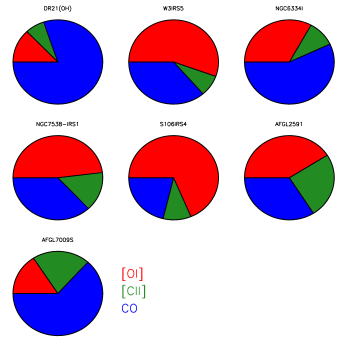
Figure 19: Cooling fractions for a sample of Galactic YSOs, for the main gas species discussed in this work: [O i] (red), [C ii] (green) and CO (blue). The fractions are listed in Table 12.

Table 12: Line luminosities as fractions of the total IR line luminosity $L_{\rm LIR}$ for [O i], [C ii] and CO. The last column gives the ratio of total IR line luminosity to total IR luminosity $L_{\rm LIR}$/$L_{\rm TIR}$.

Source ID	$L_{\rm[OI]}$	$L_{\rm[CII]}$	$L_{\rm CO}$	$L_{\rm LIR}$
	($L_{\rm LIR}$)	($L_{\rm LIR}$)	($L_{\rm LIR}$)	($L_{\rm TIR}$)
DR 21(OH)	0.13	0.07	0.81	0.003
W3 IRS5	0.55	0.08	0.36	0.002
NGC 6334I	0.33	0.10	0.57	0.0005
NGC 7538 IRS1	0.48	0.15	0.37	0.001
S 106 IRS4	0.68	0.10	0.21	0.003
AFGL 2591	0.41	0.25	0.34	0.0004
AFGL 7009S	0.16	0.21	0.64	0.001

Appendix F CO rotational diagrams fitted with admixture of LTE gas components

Another empirical description of CO rotational diagrams invokes an admixture of gas components with temperatures described by $d\,N/d\,T$ = $aT^{-b}$, over a temperature interval $T_{\rm min}$ < T < $T_{\rm max}$; such power-law distribution of temperatures has been used to successfully model rotational diagrams for both H₂ (Neufeld & Yuan, 2008) and CO (Neufeld, 2012; Manoj et al., 2013). In the limit of optically thin LTE gas and following Neufeld & Yuan (2008) and Neufeld (2012):

$$\frac{N_{J}}{g_{J}}=-\frac{N_{\rm CO}}{k/hcB}\left[\frac{b-1}{T^{1-b}_{\rm min}-T^{1-b}_{\rm max}}\right]\left[\frac{\Gamma(b,z_{1})-\Gamma(b,z_{2})}{E_{J}}\right],$$ (4)

where $b$ is the power law index, $z_{1}\equiv E_{J}/kT_{\rm min}$, $z_{2}\equiv E_{J}/kT_{\rm max}$ and $\Gamma(b,z_{i})$ is the upper incomplete gamma function. The function in Eq. 4 can be fitted to the observed rotational diagrams, with free parameters $b$, $N_{\rm CO}$, $T_{\rm min}$ and $T_{\rm max}$. Given that for the SPIRE CO transitions 55.3 $\leq E_{J}({\rm K})\leq$ 503.1, our fit solutions are insensitive to the value of $T_{\rm max}$, which is thus kept fixed at $T_{\rm max}$ = 5000 K; they are however sensitive to the value of $T_{\rm min}$ (lower limit $T_{\rm min}$ = 4 K).

Figure 20 shows the temperature power-law fits to the rotational diagrams for the YSO sample; fit parameters are listed in Table 13. The power-lax index is typically $b$ $\sim$ 3.2 (range 2.6 $-$ 4.4), consistent with literature values (Neufeld, 2012; Manoj et al., 2013). For the other two parameters we obtain: $N_{\rm CO}$ $\sim$ 9.5 $\times 10^{54}$ molecules (1 $-$ 23 $\times 10^{54}$ molecules) and $T_{\rm min}$ $\sim$ 23 K (10 $-$ 42 K). The total amount of CO is similar to that derived from the two-temperature model (Sect. 7.3.1). For one object the minimum temperature is not well constrained (N 81, Fig. 20 bottom row). For 10 out of 13 objects, a two-temperature model provides a better fit in terms of minimised $\chi^{2}$, likely a reflection of the larger number of free parameters.

While gas with temperatures over a continuum range may seem a reasonable premise, the competing processes of gas cooling and heating are likely to favour and give rise to gas with more restricted conditions. This is in fact what leads to the predominance of the different ISM phases. Therefore, the CO emission is perhaps more likely to be dominated by a few components with a temperature spread over a relatively small range.

Table 13: Fit parameters to the observed CO rotational diagrams (CO (4$-$3) to CO (13$-12$)), using a temperature power-law distribution characterised by a power-lax index $b$, total number of CO molecules $N_{\rm CO}$, and minimum temperature $T_{\rm min}$. For IRAS05328$-$6827 and LMC 053705$-$694741 the fits are very uncertain. Also listed are $\chi^{2}$ and number of degrees of freedom $N_{\rm f}$ for each fit.

Source ID	$b$	$\log N_{\rm CO}$	$T_{\rm min}$	$\chi^{2}$	$N_{\rm f}$
		(mol)	(K)
LMC YSOs
IRAS 04514$-$6931	2.8$\pm$0.1	54.94$\pm$0.23	11.1$\pm$ 3.9	19.4	7
IRAS 05328$-$6827	3.2$\pm$1.9	54.41$\pm$0.43	20.8$\pm$ 19.8	0.6	1
LMC 053705$-$694741	3.6$\pm$0.6	55.32$\pm$0.43	9.6$\pm$ 4.9	2.0	1
N113 YSO3	3.0$\pm$0.2	55.30$\pm$0.08	19.4$\pm$ 2.8	6.9	7
SAGE 045400.9$-$691151.6	4.4$\pm$0.7	55.00$\pm$0.04	38.8$\pm$ 4.3	4.9	6
SAGE 051351.5$-$672721.9	4.1$\pm$0.5	54.23$\pm$0.04	41.6$\pm$ 4.1	8.5	7
SAGE 052202.7$-$674702.1	3.0$\pm$0.3	54.32$\pm$0.09	26.9$\pm$ 5.3	9.1	7
SAGE 052212.6$-$675832.4	3.5$\pm$0.3	55.18$\pm$0.07	21.8$\pm$ 2.8	7.4	6
SAGE 053054.2$-$683428.3	3.3$\pm$0.3	54.43$\pm$0.06	31.0$\pm$ 4.4	7.1	6
ST 01	3.0$\pm$0.2	54.98$\pm$0.15	13.9$\pm$ 3.2	10.3	7
N113 YSO-1	2.7$\pm$0.1	55.36$\pm$0.07	21.4$\pm$ 3.1	3.5	7
SMC YSOs
IRAS 00464$-$7322	3.1$\pm$0.3	54.15$\pm$0.07	27.2$\pm$ 4.5	7.0	6
IRAS 00430$-$7326	3.0$\pm$0.2	54.00$\pm$0.09	25.6$\pm$ 4.3	7.1	7
N 81	2.7$\pm$0.2	55.26$\pm$0.13	4.0	8.8	6
SMC 012407$-$730904	2.6$\pm$0.1	54.74$\pm$0.16	14.4$\pm$ 4.1	12.5	7

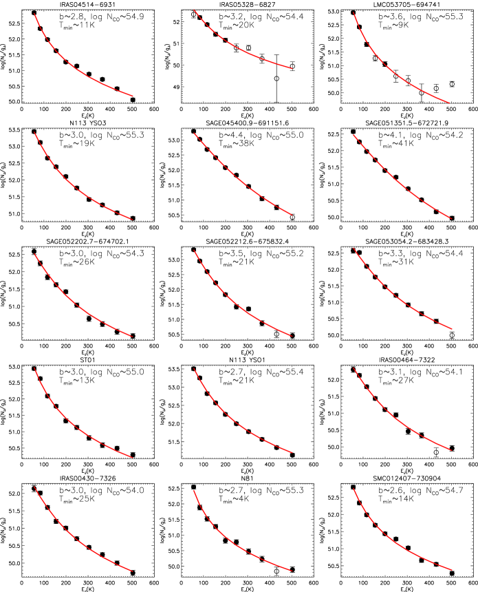
Figure 20: CO rotational diagrams for the Magellanic YSO target sample (symbols as in Fig. 6). The data are fitted by a temperature power-law distribution characterised by a power-law index $b$, a total number of CO molecules $N_{\rm CO}$ and a minimum temperature $T_{\rm min}$ (solid red lines). Approximate fit parameters are labelled in each panel; full fit results are listed in Table 13.

References

- Altieri & Vavrek (2013) Altieri B., Vavrek R., (Eds.), 2013, PACS Observer’s Manual v.2.5.1, Herschel Explanatory Supplement vol. IV, HERSCHEL-HSC-DOC-0832
- Anderl et al. (2013) Anderl S., Guillet V., Pineau des Forêts G., Flower R.D., 2013, A&A, 556, 69
- Bally (2016) Bally J., 2016, ARA&A, 54, 491
- Battersby et al. (2011) Battersby C. et al., 2011, A&A, 535, 128
- Bekki & Chiba (2007) Bekki K., Chiba M., 2007, MNRAS, 381, 16
- Bernard-Salas et al. (2012) Bernard-Salas J. et al., 2012, A&A, 538, 37
- Beuther et al. (2007) Beuther H., Churchwell E.B., McKee C.F., Tan J.C., 2007, in “Protostars and Planets V”, eds. B. Reipurth, D. Jewitt, and K. Keil, University of Arizona Press, Tucson
- Boley et al. (2013) Boley P.A. et al., 2013, A&A, 558, 24
- Bozzetto et al. (2017) Bozzetto L.M. et al., 2017, ApJS, 230, 2
- Breen et al. (2013) Breen S.L., Lovell J.E.J., Ellingsen S.P., Horiuchi S., Beasley A.J., Marvel K., 2013, MNRAS, 432, 1382
- Carlos Reyes et al. (2015) Carlos Reyes R.E., Reyes Navarro F.A., Meléndez J., Steiner J., Elizalde F., 2015, RMxAA, 51, 135
- Chen et al. (2009) Chen C.-H.R., Chu Y.-H., Gruendl R.A., Gordon K.D., Heitsch F., 2009, ApJ, 695, 511
- Chevance et al. (2016) Chevance M. et al., 2016, A&A, 590, 36
- Choudhury et al. (2018) Choudhury S., Subramaniam A., Cole A.A., Sohn Y.-J., 2018, MNRAS, 475, 4279
- Chu et al. (2003) Chu Y.-H., Chen C.-H.R., Danforth C., Dunne B.C., Gruendl R.A., Nazé Y., Oey M.S., Points S.D., 2003, AJ, 125, 2098
- Clegg et al. (1996) Clegg P.E. et al.,1996, A&A 315, 38
- Cormier et al. (2015) Cormier D. et al., 2015, A&A, 578, 53
- Cormier et al. (2019) Cormier D. et al., 2019, A&A, 626, 23
- de Wit et al. (2009) de Wit W.J. et al., 2009, A&A, 494, 157
- de Wit et al. (2011) de Wit W.J., Hoare M.G., Oudmaijer R.D., Nürnberger D.E.A., Wheelwright H.E., Lumsden S.L., 2011, A&A, 526, 5
- Ellingsen et al. (2011) Ellingsen S. P., Breen S.L., Caswell J.L., Quinn L.J., Fuller G.A., 2010, MNRAS, 404, 77
- Fish (2007) Fish V.L., 2007, in International Astronomical Union Symposium No. 242, eds. J.M. Chapman & W.A. Baan, p. 71
- Flower & Pineau des Forêts (2015) Flower D.R., Pineau des Forêts G., 2015, A&A, 578A, 63
- Fukui et al. (2015) Fukui Y. et al., 2015, ApJ, 807, 4
- Fukui et al. (2017) Fukui Y. et al., 2017, PASJ, 69, 5
- Fulton et al. (2016) Fulton T. et al., 2016, MNRAS, 458, 1977
- Gibb et al. (2004) Gibb E.L., Whittet D.C.B., Boogert A.C.A., Tielens A.G.G.M., 2004, ApJS, 151, 35
- Goicoechea et al. (2012) Goicoechea J.R. et al., 2012, A&A, 548, 77
- Goldsmith & Langer (1999) Goldsmith P.F., Langer W.D., 1999, ApJ, 517, 209
- Gordon et al. (2011) Gordon K. D. et al., 2011, AJ, 142, 102
- Graczyk et al. (2014) Graczyk D. et al., 2014, ApJ, 780, 59.
- Green et al. (2008) Green J.A et al., 2008, MNRAS, 385, 948
- Green et al. (2013) Green J.D et al., 2013, ApJ, 770, 123
- Green et al. (2016) Green J.D. et al., 2016, AJ, 151, 75
- Griffin et al. (2010) Griffin M.J. et al., 2010, A&A, 518, 3
- Gruendl & Chu (2009) Gruendl R.A., Chu Y.-H., 2009, ApJS, 184, 172
- Gry et al. (2003) Gry C. et al., 2003, "The ISO Handbook, Volume III - LWS - The Long Wavelength Spectrometer", European Space Agency, eds. Müller T.G., Blommaert J.A.D.L., García-Lario P.
- Guzmán et al. (2012) Guzmán A.E., Garay G., Brooks K. J., Voronkov M.A., 2012, ApJ, 753, 51
- Hilditch et al. (2005) Hilditch R.W., Howarth I.D., Harries T.J., 2005, MNRAS, 357, 304
- Hoare (2005) Hoare M.G., 2005, AP&SS, 295, 203
- Hollenbach & McKee (1989) Hollenbach D., McKee C.F., 1989, ApJ, 342, 306
- Hopwood et al. (2015) Hopwood R. et al., 2015, MNRAS, 449, 2274
- Houck et al. (2004) Houck J. et al., 2004, ApJS, 154, 18
- Hughes et al. (2007) Hughes A., Staveley-Smith L., Kim S., Wolleben M., Filipović M., 2007, MNRAS, 382, 543
- Imai et al. (2013) Imai H., Katayama Y., Ellingsen S.P., Hagiwara Y., 2013, MNRAS, 432, 16
- Israel & Maloney (2011) Israel F.P. and Maloney P.R., 2011, A&A, 531, 19
- Jameson et al. (2018) Jameson K.E. et al., 2018, ApJ, 853, 111
- Jiménez-Donaire et al. (2017) Jiménez-Donaire M.J., Meeus G., Karska A., Montesinos B., Bouwman J., Eiroa C. Henning T., 2017, A&A, 605, 62
- Jones et al. (2017) Jones O.C. et al., 2017, MNRAS, 470, 3250
- Karska et al. (2013) Karska A. et al., 2013, A&A 552, 141
- Karska et al. (2014) Karska A. et al., 2014, A&A, 562, 45
- Karska et al. (2018) Karska A. et al., 2018, ApJSS, 235, 30
- Kaufman et al. (1999) Kaufman M.J., Wolfire M.G., Hollenbach D.J., Luhman M.L., 1999, ApJ, 527, 795
- Kaufman et al. (2006) Kaufman M.J., Wolfire M.G., Hollenbach D.J., 2006, ApJ, 644, 283
- Kemper et al. (2010) Kemper F. et al., 2010, PASP, 122, 683
- Kessler et al. (1996) Kessler M.F. et al., 1996, A&A 315, 27
- Kramer et al. (2004) Kramer C. et al., 2004, A&A, 424, 887
- Kristensen et al. (2017) Kristensen L.E., et al., 2017, A&A, 605, 93
- Lebouteiller et al. (2012) Lebouteiller V. et al., 2012, A&A, 548, 91
- Lee et al. (2016) Lee M.-Y., et al., 2016, A&A, 596, 85
- Lee et al. (2019) Lee M.-Y., et al., 2019, A&A, 628, 113
- Leroy et al. (2007) Leroy A. et al., 2007, ApJ , 658, 102
- Lumsden et al. (2012) Lumsden S.L., Wheelwright H.E., Hoare M.G., Oudmaijer R.D., Drew J.E., 2012, MNRAS, 424, 1088
- Madden et al. (2006) Madden S.C., Galliano F., Jones A.P., Sauvage M., 2006, A&A, 446, 877
- Manoj et al. (2013) Manoj P. et al., 2013, ApJ, 763, 83
- Manoj et al. (2016) Manoj P. et al., 2016, ApJ, 831, 69
- Meijerink et al. (2013) Meijerink R. et al., 2013, ApJ, 762, 16
- Meixner et al. (2006) Meixner M. et al., 2006, AJ, 132, 2268
- Meixner et al. (2013) Meixner M. et al., 2013, AJ, 146, 62
- Momose et al. (2001) Momose M., Tamura M., Kameya O., Greaves J.S., Chrysostomou A., Hough J.H., Morino J.-I., 2001, ApJ, 555, 855
- Mottram et al. (2014) Mottram J.C. et al., 2014, A&A, 572, 21
- Mottram et al. (2017) Mottram J.C. et al., 2017, A&A, 600, 99
- Navarete et al. (2015) Navarete F., Damineli A., Barbosa C.L., Blum R.D., 2015, MNRAS, 450, 4364
- Neufeld & Yuan (2008) Neufeld D.A., Yuan Y., 2008, ApJ, 678, 974
- Neufeld (2012) Neufeld D.A., 2012, ApJ, 749, 125
- Oberst et al. (2011) Oberst T.E. et al., 2011, ApJ, 739, 100
- Oliveira et al. (2006) Oliveira J.M., van Loon J.Th., Stanimirović S., Zijlstra A.A., 2006, MNRAS, 372, 1509
- Oliveira et al. (2009) Oliveira J.M. et al., 2009, ApJ, 707, 1269
- Oliveira et al. (2011) Oliveira J.M. et al., 2011, MNRAS, 411, 36
- Oliveira et al. (2013) Oliveira J.M. et al., 2013, MNRAS, 428, 3001
- Palagi et al. (1993) Palagi F., Cesaroni R., Comoretto G., Felli M., Natale V., 1993, A&AS, 101, 153
- Pereira-Santaella et al. (2013) Pereira-Santaella M. et al., 2013, ApJ, 768, 55
- Pietrzyński et al. (2013) Pietrzyński G. et al., 2013, Nature, 495, 76
- Pilbratt et al. (2010) Pilbratt G.L. et al., 2010, A&A, 518, L1
- Poglitsch et al. (2010) Poglitsch A. et al., 2010, A&A, 518, L2
- Robitaille et al. (2006) Robitaille T.P., Whitney B.A., Indebetouw R., Wood K., Denzmore P., 2006, ApJS, 167, 256
- Robitaille (2017) Robitaille T. P., 2017, A&A, 600, 11
- Röllig et al. (2007) Röllig M. et al, 2007, A&A, 467, 187
- Roman-Duval et al. (2014) Roman-Duval J. et al., 2014, ApJ, 797, 86
- Rubin et al. (2009) Rubin D. et al., 2009, A&A, 494, 647
- Ruffle et al. (2015) Ruffle P.M.E. et al., 2015, MNRAS, 451, 3504
- Russell & Dopita (1992) Russell S.C., Dopita M.A., 1992, ApJ, 384, 508
- Salgado et al. (2016) Salgado F., Berné O., Adams J.D., Herter T.L., Keller L.D., Tielens A.G.G.M., 2016, ApJ, 830, 11
- Sandstrom et al. (2012) Sandstrom K.M. et al., 2012, ApJ, 744, 20
- Schaefer (2008) Schaefer B.E., 2008, AJ, 135, 112
- Schöier et al. (2005) Schöier F.L., van der Tak F.F.S., van Dishoeck E.F., Black J.H., 2005, A&A, 432, 369
- Seale et al. (2009) Seale J.P. , Looney L.W., Chu Y.-H., Gruendl R.A., Brandl B., Chen C.-H.R., Brandner W., Blake G.A., 2009, ApJ, 699, 150
- Seale et al. (2011) Seale J.P., Looney L.W., Chen C.-H.R., Chu Y.-H., Gruendl R.A., 2011, ApJ, 727, 36
- Seale et al. (2014) Seale J.P. et al., 2014, AJ, 148, 124
- Sewiło et al. (2010) Sewiło M. et al., 2010, A&A, 518, 73
- Sewiło et al. (2013) Sewiło M. et al., 2013, ApJ, 778, 15
- Sewiło et al. (2018) Sewiło M. et al., 2018, ApJ, 853, L19
- Shimonishi et al. (2010) Shimonishi T., Onaka T., Kato D., Sakon I., Ita Y., Kawamura A., Kaneda H., 2010, A&A, 514, 12
- Shimonishi et al. (2016) Shimonishi T. et al. 2016, ApJ, 827, 72
- Spinoglio et al. (2012) Spinoglio L. et al., 2012, ApJ, 758, 108
- Stock et al. (2015) Stock D.J., Wolfire M.G., Peeters E., Tielens A.G.G.M., Vandenbussche B., Boersma C., Cami J., 2015, A&A, 579, 67
- Sutherland et al. (2013) Sutherland R., Dopita M., Binette L., Groves B., 2013, Astrophysics Source Code Library, record ascl:1306.008
- Tielens et al. (1984) Tielens A.G.G.M., Allamandola L.J., Bregman J., Goebel J., D’Hendecourt L., Witteborn F.C., 1984, ApJ, 287, 697
- Tielens & Hollenbach (1985) Tielens A.G.G.M., Hollenbach D., 1985, ApJ, 291, 722
- Tsuge et al. (2019) Tsuge K. et al., 2019, ApJ, 871, 44
- Valtchanov (2017) Valtchanov I. (Ed.), 2017, SPIRE Handbook v3.1, Herschel Explanatory Supplement vol. IV, HERSCHEL-HSC-DOC-0798
-
Vandenbussche (2011)
Vandenbussche B., 2011, PACS spectroscopy performance and calibration,
http://herschel.esac.esa.int/twiki/pub/Public/PacsCalibrationWeb/Pacs
SpectroscopyPerformanceAndCalibrationv24.pdf - van der Tak et al. (2007) van der Tak F.F.S., Black J.H., Schöier F.L., Jansen D.J., van Dishoeck E.F., 2007, A&A, 468, 627
- van der Tak et al. (2013) van der Tak F.F.S. et al, 2013, A&A, 554, 83
- van Dishoeck et al. (2011) van Dishoeck E.F. et al., 2011, PASP, 123, 138
- van Dishoeck et al. (2013) van Dishoeck E.F., Herbst E., Neufeld D.A., 2013, ChRv, 113, 9043,
- van Loon et al. (2005) van Loon J.Th. et al., 2005, MNRAS, 364, 71
- van Loon et al. (2010a) van Loon J.Th. et al., 2010a, AJ, 139, 68
- van Loon et al. (2010b) van Loon J.Th. et al., 2010b, AJ, 139, 1553
- Wampfler et al. (2013) Wampfler S.F. et al., 2013, A&A, 552, 56
- Ward et al. (2016) Ward J.L., Oliveira J.M., van Loon J.Th., Sewiło M., 2016, MNRAS, 455, 2345
- Ward et al. (2017) Ward J.L., Oliveira J.M., van Loon J.Th., Sewiło M., 2017, MNRAS, 464, 1512
- Wendker et al. (1991) Wendker H.J., Higgs L.A., Landecker T.L., 1991, A&A, 241, 551
- Werner et al. (2004) Werner M. et al., 2004, ApJS, 154, 1
- White et al. (2010) White G.J. et al., 2010, A&A, 518, 114
- Whitney et al. (2008) Whitney B.A et al., 2008, AJ, 136, 18
- Wilson et al. (2003) Wilson T.L., Boboltz D.A., Gaume R.A., Megeath S.T., 2003, ApJ, 597, 434
- Woods et al. (2011) Woods P.M. et al., 2011, MNRAS, 411, 1597
- Yang et al. (2010) Yang B., Stancil P.C., Balakrishnan N., Forrey R.C., 2010, ApJ, 718, 1062
- Yang et al. (2017) Yang Y.-L., Evans N.J.II, Green J.D., Dunham M.M., Jørgensen J.K., 2017, ApJ, 835, 259
- Yang et al. (2018) Yang Y.-L. et al., 2018, ApJ, 860, 174
- Yıldız et al. (2013) Yıldız U.A. et al., 2013, A&A, 556, 89