Turbulence and Transport During Guide-Field Reconnection at the Magnetopause

Abstract

We analyze the development and influence of turbulence in three-dimensional particle-in-cell simulations of guide-field magnetic reconnection at the magnetopause with parameters based on observations of an electron diffusion region by the Magnetospheric Multiscale (MMS) mission. Along the separatrices the turbulence is a variant of the lower hybrid drift instability (LHDI) that produces electric field fluctuations with amplitudes much greater than the reconnection electric field. The turbulence controls the scale length of the density and current profiles while enabling significant transport across the magnetopause despite the electrons remaining frozen-in to the magnetic field. Near the X-line the electrons are not frozen-in and the turbulence, which differs from the LHDI, makes a significant net contribution to the generalized Ohm’s law through an anomalous viscosity. The characteristics of the turbulence and associated particle transport are consistent with fluctuation amplitudes in the MMS observations. However, for this event the simulations suggest that the MMS spacecraft were not close enough to the core of the electron diffusion region to identify the region where anomalous viscosity is important.

I Introduction

As the central agent of the Dungey cycle Dungey (1961), magnetic reconnection controls the interaction between the plasmas of the magnetosphere and the solar wind. The necessary change in magnetic topology occurs at an X-line embedded within a small diffusion region where kinetic effects become significant enough to make ideal magnetohydrodynamics an inadequate description of the dynamics, while the energy stored in the reconnecting fields dissipates on larger scales, producing flows, heat, and non-thermal particles. The best understanding of the details of magnetospheric reconnection springs from the interplay between in situ observations and numerical simulations incorporating the necessary kinetic physics. The quartet of spacecraft comprising the Magnetospheric Multiscale (MMS) mission Burch et al. (2016a) make temporally and spatially resolved measurements within diffusion regions but can only sample along individual trajectories. Their data complement numerical simulations that provide synoptic overviews of reconnection but must cope with computational limitations.

Because of the resources required for fully three-dimensional domains, many reconnection simulations treat a reduced geometry in which variations in one direction are ignored. (In the $LMN$ coordinate system used here, in which $L$ parallels the direction of the reconnecting magnetic field and $N$ parallels the inflow direction, the invariant direction is $M$, which points perpendicular to both $L$ and $N$. At the equator of the noon-midnight meridian, $L$ points north-south, $M$ east-west, and $N$ radially.) This two-dimensional simplification eliminates fluctuations with non-zero wavenumber $k_{M}$ and hence inhibits the development of turbulence, which is typically driven by strong $M$-aligned currents along the magnetopause. Reconnection in this limit is typically laminar, although current-driven instabilities along the separatrices can produce intense parallel electric fields Cattell et al. (2005); Lapenta et al. (2011).

However, MMS observations of magnetopause reconnection have shown that turbulence does in fact develop near the X-line, suggesting that three-dimensional computational domains are necessary Graham et al. (2017); Ergun et al. (2017). Motivated by MMS observations of nearly anti-parallel (i.e., $B_{M}\approx 0$) reconnection Burch et al. (2016b), simulations demonstrated that the strong gradient in density between the magnetosheath and magnetosphere triggers a variant of the lower-hybrid drift instability Price et al. (2016, 2017); Le et al. (2017). The turbulence appeared at both the X-line and along the magnetic separatrices and had characteristic scale $k\rho_{e}\sim(m_{e}T_{e}/m_{i}T_{i})^{0.25}$, with $\rho_{e}$ the electron Larmor radius. It relaxed the magnetopause density gradient while producing significant anomalous resistivity and viscosity in the diffusion region. The accompanying fluctuations in the out-of-plane electric field, $E_{M}$, had amplitudes much greater than the steady electric field driving reconnection.

The magnetic configuration during magnetopause reconnection can also include a significant $B_{M}$, or guide-field, component and there are reasons to suspect that this additional component may alter the conclusions drawn from near-anti-parallel events. The classic lower-hybrid drift instability is known to be suppressed by the presence of magnetic shear, which should be strong when the guide field is significant Huba et al. (1982). In addition, magnetization of the electrons by the guide field, even within the diffusion region where the reconnecting component of the field vanishes, can affect the development of anomalous dissipation terms that rely on correlations between fluctuating quantities.

On 2015 December 08 at about 11:20 UT MMS passed close to the X-line of a guide-field ($B_{M}\approx B_{L}$) reconnection event at the magnetopause Burch and Phan (2016). It observed a bifurcated current system accompanied by significant fluctuations in the current density, magnetic field, and electric field. For the perpendicular components of the electric field those fluctuations were near the local lower hybrid frequency while the parallel component included higher frequencies that reached amplitudes of $\approx 30$ mV/m and peaked on the magnetospheric side of the layer Ergun et al. (2017). The MMS observations also reveal that electrons are often frozen-in to the fluctuations Graham et al. (2019). Previous simulations based on this event and two others Le et al. (2018) revealed the development of drift-wave fluctuations as well as noting the accompanying enhancement of cross-field electron transport and parallel heating. However, whether the strong turbulence measured at the magnetopause actually drives transport or produces the necessary dissipation remain open questions as previous three-dimensional simulations of reconnection-driven turbulence did not adequately address the impact of frozen-in electrons on transport Price et al. (2016, 2017); Le et al. (2017, 2018). The turbulence that develops in the strong density gradient across the magnetopause has characteristic time scales that are intermediate between the electron and ion gyrofrequencies. As a consequence, unless electrons resonate with waves they typically remain magnetized and frozen-in. Resonance occurs either through parallel streaming in fluctuations with a finite $k_{\parallel}$ with respect to the ambient magnetic field or through drifts due to the magnetic field gradient Davidson et al. (1976). It is known that irreversible transport of plasma density and momentum requires a resonant interaction between electric fields and particles Drake and Lee (1981). Turbulence with frozen-in electrons greatly reduces the dissipation described by the generalized Ohm’s law.

In this paper we present three-dimensional simulations of reconnection with initial conditions reflective of the MMS event described in Burch and Phan (2016). Surprisingly, because of the relaxation of the cross-magnetopause density gradient and despite the guide field stabilization, LHDI still develops along the separatrices in a manner reminiscent of the nearly anti-parallel case. At the X-line, on the other hand, the LHDI is stabilized. Nevertheless, a different instability develops that produces significant anomalous dissipation. Finally, we establish that irreversible transport at the magnetopause can occur, even when the electrons remain frozen-in, due to the strong vortical motions that effectively create nonlinear fluid resonances. Section II describes the parameters of the simulation, section III describes the results, while section IV offers our conclusions.

II Simulations

We perform simulations with the particle-in-cell code p3d Zeiler et al. (2002). It employs units based on a reference magnetic field strength $B_{0}$ and density $n_{0}$ which then define an Alfvén speed $v_{A0}=\sqrt{B_{0}^{2}/4\pi m_{i}n_{0}}$. Lengths are normalized to the ion inertial length $d_{i}=c/\omega_{pi}$, where $\omega_{pi}=\sqrt{4\pi n_{0}e^{2}/m_{i}}$ is the ion plasma frequency, and times to the ion cyclotron time $\Omega_{i0}^{-1}=m_{i}c/eB_{0}$. Electric fields and temperatures are normalized to $v_{A0}B_{0}/c$ and $m_{i}v_{A0}^{2}$, respectively.

The initial conditions closely mimic those observed by MMS during the diffusion region encounter on 8 December 2015 described in Burch and Phan (2016). The particle density $n$, reconnecting component of the magnetic field $B_{L}$, guide field component $B_{M}$, and ion temperature $T_{i}$ vary as functions of the $N$ coordinate with hyperbolic tangent profiles of width 1. The asymptotic values of $n$, $B_{L}$, $B_{M}$, and $T_{i}$ are 0.222, 1.59, -0.659, and 3.19 in the magnetosphere and 1.00, -1.00, -0.414, and 1.59 in the magnetosheath. Pressure balance determines the profile of the electron temperature $T_{e}$, subject to the constraint that its asymptotic value in the magnetosphere is 0.664. (In the asymptotic magnetosheath $T_{e}$ is thus 0.159 and, as a consequence, the asymptotic electron pressures differ by less than 10%.) The shear angle between the asymptotic magnetic fields is $\approx 135^{\circ}$.

Rather than allow reconnection to develop from noise, we apply an initial perturbation that is uniform in the $M$ direction. Since such a perturbation imposes a preferred direction for the development of the X-line, we have rotated the system so that the $M$ axis bisects the angle formed by the asymptotic magnetic fields. Previous work Swisdak and Drake (2007); Hesse et al. (2013); Liu et al. (2015) suggests that this choice mimics the direction that the X-line would naturally choose in the absence of a perturbation. The initial conditions are not an exact Vlasov equilibrium, although they are in force balance prior to the perturbation. The system adjusts once the simulation begins and reaches a near-steady-state configuration before the turbulence and reconnection considered here become important.

We present results from both two-dimensional (in the $\partial/\partial M=0$ sense) and three-dimensional simulations with box sizes of $(L_{L},L_{N})=(40.96,20.48)$ and $(L_{L},L_{M},L_{N})=(40.96,20.48,20.48)$, respectively. The boundary conditions are periodic in all directions. In order to reduce the computational expense, but still separate the characteristic scales associated with the two species, the ion-to-electron mass ratio is chosen to be $100$. Spatial gridpoints have a separation of $\Delta=0.016$ while the smallest physical scale, the Debye length in the magnetosheath, $\approx 0.04$. We employ $50$ particles per cell when $n=1$, which implies $\approx 11$ particles per cell in the low-density magnetosphere. To mitigate the resulting noise, our analysis sometimes includes averages over multiple cells.

The velocity of light in the simulations is $c=15$ so that $\omega_{pe}/\Omega_{ce}=1.5$ in the asymptotic magnetosheath and $\approx 0.4$ in the asymptotic magnetosphere while the values derived from the MMS data are larger ($\approx 40$ and 10, respectively). As a result, the ratio of the Debye length to other typical lengthscales is larger in the simulations, which may tend to suppress very short wavelength electrostatic instabilities Jara-Almonte et al. (2014).

III Results

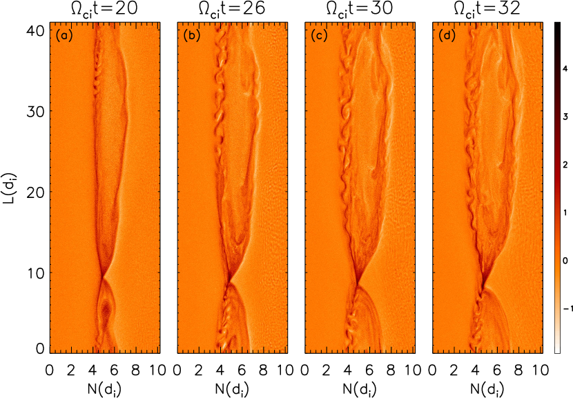
Figure 1: Images of $J_{eM}$, the dawn-dusk electron current density, in a single $L-N$ plane at four times showing the development of turbulence. The panels share the same normalization, which is given by the color bar.

Figure 1 displays images of $J_{eM}$, the dawn-dusk electron current density, from an $L-N$ slice of the three-dimensional simulation at four times during which reconnection is occurring at an approximately uniform rate of 0.11 in normalized units. In each panel the magnetosphere (strong field, low density) is to the left and the magnetosheath (weak field, high density) is to the right. For asymmetric configurations such as this the reconnection of equal amounts of magnetic flux from the two plasmas forces the island to bulge into the weaker field region. At the time shown in the first panel, turbulent features have clearly developed along the downstream magnetospheric separatrix ($30\lesssim L\lesssim 40$ and $N\approx 4$). These arise from the version of the lower-hybrid drift instability previously seen in simulations of anti-parallel magnetopause reconnection by others Price et al. (2016, 2017); Le et al. (2017). The turbulence expands as the simulation progresses, eventually appearing along all of both separatrices, with the exception of a small region near the X-line. The MMS observations of this event reveal a double peak in $J_{M}$, primarily field-aligned, at the closest approach to the X-line. Such a bifurcation in $J_{M}$, also mostly field-aligned, only occurs in the simulation data at distances $\lesssim 1d_{i}$ ($10d_{e}$ for the mass ratio used here) downstream from the X-point and within the region affected by LHDI. Close to the X-line, in contrast, cross-field currents become important. These points suggest that the MMS spacecraft did not cross through the region where, as will be shown below, LHDI is stabilized. The two-dimensional companion simulation (not shown) reconnects flux at a similar rate but remains laminar.

Figure 2 shows $J_{eM}$ at $t=26$ the approximate time when the turbulent fluctuations on the separatrices reach their largest amplitude. The first panel is identical to panel (b) of Figure 1 save for the addition of the two dashed lines giving the locations of the $M-N$ planes shown in panels (b) and (c). In the first, from the center of the island of reconnected flux, the turbulence at both separatrices is clearly visible although notably stronger on the magnetospheric side due to, as will be discussed below, the stronger density gradient there. The instability is the same variant of LHDI observed in Price et al. (2017) and Le et al. (2017) in simulations of anti-parallel magnetopause reconnection. In a narrow current sheet – one with width less than of order the ion gyroradius – theory and simulations suggest a longer-wavelength version of the classic LHDI develops with the relative drift of electrons and ions in the $M$ direction supplying the necessary free energy Winske (1981); Daughton (2003). The excited wavenumbers satisfy $(m_{e}T_{e}/m_{i}T_{i})^{0.25}\lesssim k_{M}\rho_{e}\lesssim 1$, where $\rho_{e}$ is the thermal electron Larmor radius. Using the temperatures from the time of peak power shown in Figure 2, this can be written as a condition on the wavelength: $0.24\lesssim\lambda_{M}/d_{i}\lesssim 1.64$. The structure in panel (b) has $\lambda_{M}\approx 0.9d_{i}$ and falls within the expected range. (This agreement should be qualified by noting that the system includes many strong asymmetries while most analyses of LHDI assume symmetric Harris-type current sheets.)

However, a similar cut through the X-line, panel (c), exhibits minimal turbulence at the wavelengths expected from LHDI. This is in sharp contrast to the system with near-anti-parallel reconnection where LHDI is observed both along the separatrices and on the magnetosphere side of the X-line. (Below we will show that there are perturbations at longer wavelengths unrelated to LHDI.) The key difference is the presence of the guide field. Classic LHDI with $k_{\perp}\rho_{e}\sim 1$ and $k_{\parallel}=0$ is known to be stabilized by magnetic shear at the location of the maximum density gradient Huba et al. (1982). Stabilization occurs when $k_{\parallel}v_{te}$, where $v_{te}$ is the electron thermal speed, exceeds $\omega$; for classic LHDI, one can show that implies stabilization occurs for a magnetic field rotation of $\Delta\theta\gtrsim\sqrt{m_{e}/m_{i}}$.

Figure 3 shows the profiles of $B_{L}$, $B_{M}$, and $n_{e}$ as functions of $N$ through both the X-line and the separatrix along the dashed lines in Figure 2a. At the X-line the largest density gradient coincides with a sharp change in $B_{L}$ (length scale $\approx 0.5d_{i}$) and hence a large magnetic shear. At the separatrix, in contrast, the rotation in the magnetic field is significantly weaker (length scale $\approx 1.5d_{i}$) and, as a result, LHDI is not stabilized there. (Although Huba et al. (1982) considered the classic form of LHDI and not the longer wavelength variant discussed here the stabilizing influence of magnetic shear is expected to be similar.) Figure 3 also shows the reason for the relative strengths of the LHDI at the magnetopause and magnetosheath separatrices: the density gradient at the former ($N\approx 4$) greatly exceeds that at the latter ($N\approx 7$). While the LHDI is stabilized around the X-line in this guide-field reconnecting system, we show below that there is a long-wavelength instability driven by the gradient in the current density that impacts Ohm’s law Che et al. (2011).

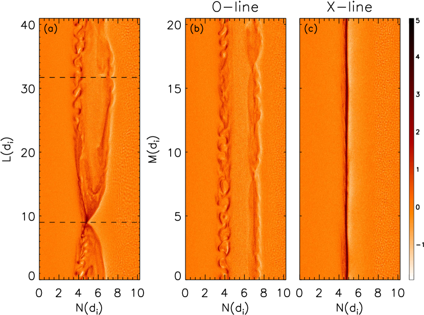
Figure 2: Images of $J_{eM}$ in different planes. Panel (a) is identical to panel (b) of Figure 1 and shows the current density in an $L-N$ plane at $t=26$. Panels (b) and (c) show $J_{eM}$ in an $M-N$ plane at the locations indicated by the dotted lines in panel (a), the former through the center of the island of reconnected flux and the latter through the X-line.

As in the anti-parallel reconnecting system, LHDI broadens the current sheet. However, due to the magnetic shear stabilization, the broadening only occurs on the separatrices and not at the X-line. Figure 4 shows the density scale length, $L_{n}=n/|\bm{\nabla}n|$ as a function of time on cuts in the $N$ direction in both the two-dimensional and three-dimensional simulations. At the X-line, where the LHDI is suppressed, the evolution of $L_{n}$ is remarkably similar in both cases, gradually shrinking from its initial value until reconnection begins ($t\approx 15$) and then remaining roughly constant. At the separatrix, in contrast, the two- and three-dimensional simulations only agree until the amplitude of the LHDI becomes significant, at which point the three-dimensional current layer broadens and gradually continues to thicken for the remainder of the run.

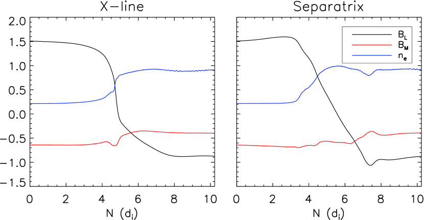
Figure 3: Cuts in the $N$ direction through the X-line (left) and center of the island (right) at $t=26$ and the locations given by the dashed lines in Figure 2a.

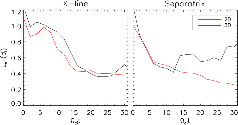
Figure 4: Density scale length $L_{n}=n/|\bm{\nabla}n|$ measured at the X-line and through the downstream separatrix as a function of time for both two-dimensional (red) and three-dimensional (black) simulations.

Despite the turbulence, magnetic flux reconnects in the two-dimensional and three-dimensional simulations at essentially the same rate. The speed at which this occurs is given by the $M$ component of the electric field, which can be expressed in terms of other quantities through the generalized Ohm’s law, a rewriting of the electron momentum equation. However, raw time series of $E_{M}$ from the simulation exhibit fluctuations, from both the turbulence and the noise inherent to PIC simulations, that are much larger in amplitude than the part of $E_{M}$ responsible for reconnection. In order to quantify the impact of turbulence on large-scale reconnection, we consider an $M$-averaged version of the generalized Ohm’s law that, in effect, coarse-grains the data. The averaged Ohm’s law is useful if the scale length of the turbulence is shorter than the length of the simulation along the $M$ direction. The LHDI develops at short scale so the averaged Ohm’s law yields an appropriate measure of the rate of reconnection (see panels (b) and (c) of Figure 2). However, a longer wavelength instability develops at the X-line (see below). This instability has a wavelength smaller, though not significantly smaller, than the domain. Consequently, the balance of the various terms in the averaged Ohm’s law is not as complete in this location as along the separatrices. A derivation is given in the Appendix.

Before discussing the impact of turbulence on how field lines break during reconnection, we digress briefly on the electron frozen-in condition in the presence of turbulence. The momentum equation for electrons is given by

$$mn\frac{d\mathbf{v}}{dt}=-en\mathbf{E}-\bm{\nabla\cdot}\mathbb{P}-en(\mathbf{v}\bm{\times}\mathbf{B})/c.$$ (1)

In a laminar system the electric field term and the Lorentz force term balance everywhere except near the X-line where the Lorentz force term vanishes and the pressure tensor term typically provides the balance Hesse et al. (1999). Stated another way, the electrons remain frozen-in everywhere except the X-line. In a system with strong turbulence it is still possible for the electrons to remain frozen-in to the fluid so that $\tilde{\mathbf{E}}\sim-(\tilde{\mathbf{v}}\bm{\times}\mathbf{B})/c$, where $\tilde{\mathbf{E}}$ and $\tilde{\mathbf{v}}$ represent turbulent quantities. Under these conditions, the contributions of the turbulence to Ohm’s law are strongly suppressed because the first and last terms on the right side of equation (1) cancel. In Figure 5 we show cuts in the $M$ direction of $E_{M}$ and $-(\mathbf{v}\bm{\times}\mathbf{B})_{M}/c$ at the same value of $L$ as in Figure 2 at the peak of the turbulence along the magnetopause separatrix ($N\approx 3.9$). The conversion from simulation to MKS units is such that the peaks in $E_{M}$ correspond to fluctuations of $\approx 20$ mV/m, which is reasonably consistent with the MMS observations Ergun et al. (2017).

The electrons remain almost completely frozen-in even though the turbulence is strong. Thus, along the separatrix the impact of the turbulence on the averaged Ohm’s law will be significantly reduced. That electrons are frozen-in to the LHDI turbulence also raises the question as to how this instability produces the transport necessary to broaden the density profile as shown in Fig. 4. Resonant interactions that break the frozen-in condition of electrons are required for real, irreversible transport to occur Drake and Lee (1981). The data from MMS during its magnetopause crossing also suggest that electrons remained frozen-in, reducing the impact of the LHDI on Ohm’s law Graham et al. (2019). This cancellation was not adequately explored in earlier magnetopause simulations Price et al. (2016, 2017); Le et al. (2017).

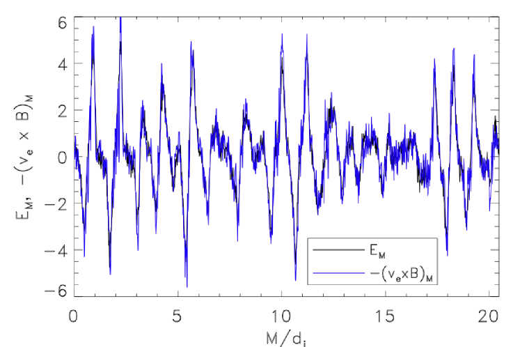
Figure 5: Cuts in the $M$ direction at the $L$ value of the dashed line crossing the separatrix in Figure 2 and $N\approx 3.9$ of $E_{M}$ and $-(\mathbf{v}_{e}\bm{\times}\mathbf{B})_{M}$.

The expansion of the quantities in equation (1) in terms of mean and fluctuating terms culminates in equation (7) after the average over the $M$ direction. The equation for the reconnection electric field take the form

$$e\langle n_{e}\rangle\langle E_{M}\rangle=(\text{laminar terms})+(\text{anomalous terms})$$ (2)

The first expression on the right-hand side includes terms such as $e\langle n\rangle\langle v_{L}\rangle\langle B_{N}\rangle/c$, only involves average quantities, and describes the bulk behavior of the plasma. These terms represent the contributions to the generalized Ohm’s law from the reconnection electric field seen in both two- and three-dimensional simulations: the Lorentz force, the pressure tensor, and the fluid inertia. When turbulence does not exist or is unimportant these terms will fully balance the left-hand side of equation 2.

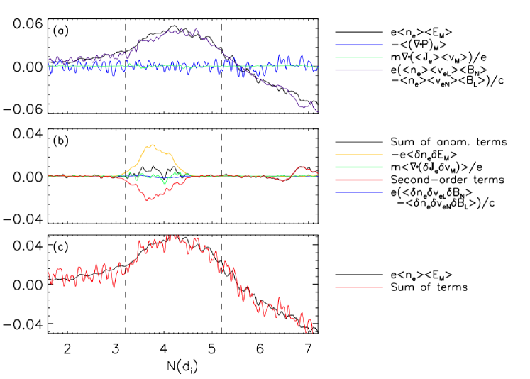
Figure 6: Cuts in the $N$ direction through the downstream separatrix for the three-dimensional simulation at $t=26$. Panel (a): The laminar terms in the $M$ component of the $M$-averaged Ohm’s law. Panel (b): The terms in the $M$-averaged Ohm’s law due to correlations in turbulent fluctuations. Panel (c): The sum of the two sides of equation 6. In each panel the vertical lines show the approximate positions of the separatrix (left) and the middle of the island (right).

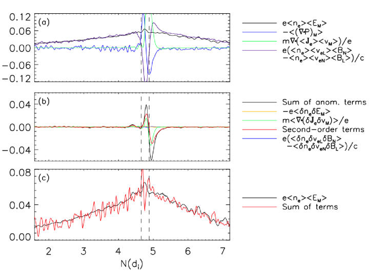
Figure 7: Cuts in the $N$ direction through the X-line for the three-dimensional simulation at $t=26$. Panel (a): The laminar terms in the $M$ component of the $M$-averaged Ohm’s law. Panel (b): The terms in the $M$-averaged Ohm’s law due to correlations in turbulent fluctuations. Panel (c): The sum of the two sides of equation 6. In each panel the vertical lines show the approximate positions of the stagnation point (left) and in-plane magnetic null (right).

The second group of terms involves averages of products of fluctuating components, which can be non-zero in the presence of correlations. One such term, $\langle\delta n\delta E_{M}\rangle$, can be interpreted as arising from an anomalous drag between electrons and protons Drake et al. (2003) while others, including $e\langle\delta n\delta v_{L}\rangle\langle B_{N}\rangle/c$ describe an anomalous viscosity associated with the turbulent transport of the $M$ component of the canonical momentum $p_{M}-eA_{M}/c$ with $B_{L}=\partial A_{M}/\partial N$, where $\mathbf{A}$ is the vector potential Che et al. (2011). For frozen-in electrons these two terms exactly cancel. All of these terms measure the contributions of the turbulence to reconnection.

In Figure 6a we show these terms as a function of $N$ for a cut through the downstream separatrix at the location indicated by the dashed line in Figure 2. Panel (a) shows the laminar terms and demonstrates, as might be expected, that the plasma is nearly frozen-in with $\mathbf{E}\approx-(\mathbf{v}\bm{\times}\mathbf{B})/c$. The other terms, representing the contributions of inertia and the pressure tensor, are negligible. (The largest component of the pressure tensor divergence, $\partial P_{MM}/\partial M$, vanishes after the averaging and hence makes no contribution.) Panel (b) shows the terms due to the turbulent fluctuations. The most significant are the yellow curve giving the anomalous resistivity and the red curve representing the six terms due to correlated fluctuations in the elements of $n\mathbf{v}\bm{\times}\mathbf{B}$. The other terms, represented by the green and blue lines, have negligible effects. The black curve shows the sum of all anomalous terms and demonstrates that, although the largest contributions are similar in amplitude to the terms shown in panel (a), there is a significant cancellation. This cancellation confirms that the electrons are basically frozen-in at this location, which is perhaps not surprising given that the LHDI wavelength exceeds the electron Larmor radius and the associated frequency is well below $\omega_{ce}$. However, seeing that frozen-in electrons leads to the cancellation of terms in Ohm’s law depends on the decomposition of the generalized Ohm’s law leading to equation 7. For instance Price et al. (2017)’s decomposition used $\mathbf{J}$ in the Lorentz force term rather than $n$ and $\mathbf{v}$. As a result, the frozen-in nature of the electrons and its impact was obscured both in this paper and others Le et al. (2017). Finally, in panel (c) the left- and right-hand sides of equation 7 are plotted, showing that the two sides balance.

Figure 7 shows a similar set of plots as Figure 6 from a cut through the X-line along the dashed line in Figure 2. The top panel shows that, unlike the separatrix cut, every term makes a significant contribution to balancing the reconnection electric field. Asymptotically the Lorentz force makes the primary contribution, but between the stagnation and X-points (left and right dashed lines, respectively) the Lorentz term reverses sign while the pressure tensor and inertial terms also contribute. Panel (b) again shows the anomalous terms. Unlike at the separatrices, the anomalous resistivity term, $-e\langle\delta n_{e}\delta E_{M}\rangle$, essentially vanishes, consistent with the stabilization of LHDI and the laminar cut shown in Figure 2(c). The summation of the anomalous terms (black line) does not vanish, indicating that the electrons are not frozen-in at this location. The balance shown in panel (c), while not as precise as in Figure 6(c), is still reasonable. The deviations are likely due to the effects of the time-dependent term in Ohm’s law, $\partial\langle J_{M}\rangle/\partial t$, which is not known to the same precision as the other terms.

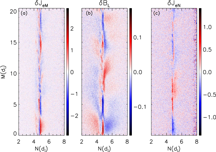
Figure 8: Images of fluctuating quantities in an $M-N$ plane through the X-line at $t=26$. In each panel white represents zero amplitude while red and blue represent positive and negative fluctuations, respectively.

What is the source of the anomalous contributions to the generalized Ohm’s law at the X-line in Figure 7(b) where the magnetic shear stabilizes LHDI? Figure 8 displays the fluctuating parts (i.e., the part remaining after subtracting off the average in the $M$ direction) of three quantities at the same time and location as panel (c) of Figure 2: $\delta J_{eM}$, $\delta B_{L}$, and $\delta J_{eN}$. The fluctuations share several characteristics with the structures reported in Ergun et al. (2017) after analysis of several MMS events. They observed fluctuations with $k_{\parallel}\neq 0$ accompanied by parallel electron flows and strong, high-frequency bursts of $E_{\parallel}$ in regions with minimal electron pressure gradients. These characteristics did not match those usually associated with LHDI, leaving them unsure of the source of the turbulence. The mode structure in the simulations is complex, but approximately two wavelengths fit into the domain. In an earlier three-dimensional simulation with half of the length of the domain in $M$ only a single wavelength of this instability appeared. The displacement of the electrons in the $N$ direction in Fig. 2(c) leads to corresponding increases and decreases in the local current $\delta J_{eM}$ in Fig. 2(a), indicating that the electron motion displaces the ambient current $J_{eM}$. That the motion is localized in $N$ in the region where the gradient in $J_{eM}$ is large suggests that this instability is driven by the current gradient Che et al. (2011). Figure 9 shows the spatial distribution of the contributions of the anomalous terms to the generalized Ohm’s law in a portion of the $L-N$ plane at $t=26$. The terms are small along the separatrices, consistent with the cuts shown in Figure 6. Near the X-line, however, there is a notable increase that is reflected in the cuts seen in Figure 7. The region of enhanced anomalous viscosity extends $\lesssim 1d_{i}$ downstream from the X-line and barely reaches the region of bifurcated $J_{M}$. The guide field also introduces an asymmetry in the $L$ direction. Close to the X-line, but outside the electron diffusion region, the anomalous contributions appear to be more significant southward of the X-line. Since MMS observations include a notable current bifurcation, the effects of anomalous viscosity are not expected to appear in its data.

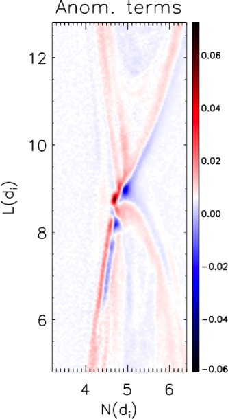
Figure 9: Image of the anomalous terms from equation 7 in a portion of the $L-N$ plane at $t=26$ showing its localization near the X-line.

In the anti-parallel reconnecting system, LHDI drove sufficient particle transport to limit the density scale length to a hybrid of the electron and ion Larmor radii both along the separatrices and on the magnetospheric side of the X-line. We now explore how the turbulence in the case of a guide field limits the density profiles. To quantify the transport we write the turbulent particle flux in the $N$ direction, discarding the component along the magnetic field $B_{N}$, as

$$\Gamma_{N\perp}=\langle\delta n\delta V_{eN,\perp}\rangle,$$ (3)

where the average is over the $M$ direction. Due to the magnetic shear stabilization around the X-line, the turbulence only controls the profiles across the separatrices (see Figure 4). On the other hand, the electrons remain frozen-in even along the separatrices so how can the electrons undergo irreversible transport, which requires a resonant interaction between the electrons and the turbulence? For turbulence with $k_{\parallel}=0$, electrons can resonantly interact with the waves through their $\bm{\nabla}B$ drift Davidson et al. (1976). However, because of the low electron temperatures in the present simulations and at the actual magnetopause, this resonance is not likely to play a role. In linear theory in this limit $\delta n$ is simply given by the electron convection along the density gradient and is $\pi/2$ out of phase with $V_{eN,\perp}$. The consequence is that the right side of equation (3) is zero unless the amplitude of the wave is changing in time. The broadening of the density profile in this limit results from rippling of the density profile and is fully reversible Drake and Lee (1981).

However, irreversible transport can occur via $\mathbf{E}\times\mathbf{B}$ trapping Kleva and Drake (1984), in which the vortical motion of the fluid is strong enough for the electron orbits perpendicular to the magnetic field to become chaotic. The result is a fluid-like rather than a kinetic resonance. The requirement to enter this regime is for the $M$ component of the $\mathbf{E}\times\mathbf{B}$ drift to exceed the wave phase speed in the electron reference frame. In Figure 10 we show a cut of the density in the $M-N$ plane in a cut through the magnetopause separatrix. At this time the density no longer exhibits the periodic displacement in the $N$ direction that characterizes the linear LHDI stability theory. The density has developed a complex turbulent structure that characterizes true diffusion. Thus, electron diffusion across the magnetopause is possible even if the electrons remain frozen-in. Cuts of the individual quantities from the right-hand side of equation 3 that exhibit the phase relationship between them, are shown in Figure 11a. Because of the nonlinear nature of the turbulence the phase relation between $\delta n/n$ and $V_{N,\perp}$ is complex but exhibits regions where the two quantities are in phase and net transport occurs. Such cuts are closely related to what spacecraft passing through a turbulent reconnecting separatrix would observe.

The flux $\Gamma_{N\perp}$ calculated from the simulation data using equation 3 is shown at $t=26$ in the $L-N$ plane in Figure 12a. For the density profiles to reach a quasi-steady-state as suggested by the data in Figure 4, the fluxes associated with the laminar motion (reconnection inflows and outflows) both perpendicular and parallel to the ambient field must balance the diffusive fluxes. This requires $\Gamma_{N\perp}\sim nV_{in}\sim 0.1nC_{AL}$, where $V_{in}\sim 0.1C_{AL}$ is the characteristic reconnection inflow speed. The turbulent fluxes in Figure 12a are sufficient to balance the laminar flows associated with reconnection, which is consistent with the quasi-steady density gradient that develops along the separatrix.

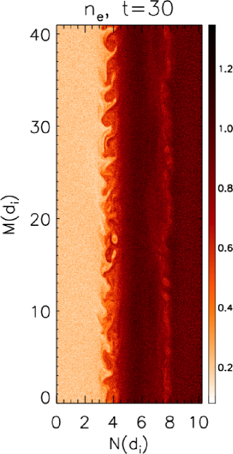
Figure 10: Electron density in the same $M-N$ plane as in Figure 2b at $t=30$ showing the development of nonlinear structures along the magnetospheric separatrix.

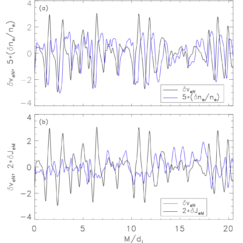
Figure 11: Cuts in the $M$ direction at the $L$ value of the dashed line crossing the separatrix in Figure 2 and $N\approx 3.9$ of: (a) $\delta n_{e}/n_{e}$ and $\delta V_{eN,\perp}$ and (b) $\delta V_{eN,\perp}$ and $\delta J_{eM}$. All quantities have been smoothed to remove high-frequency noise.

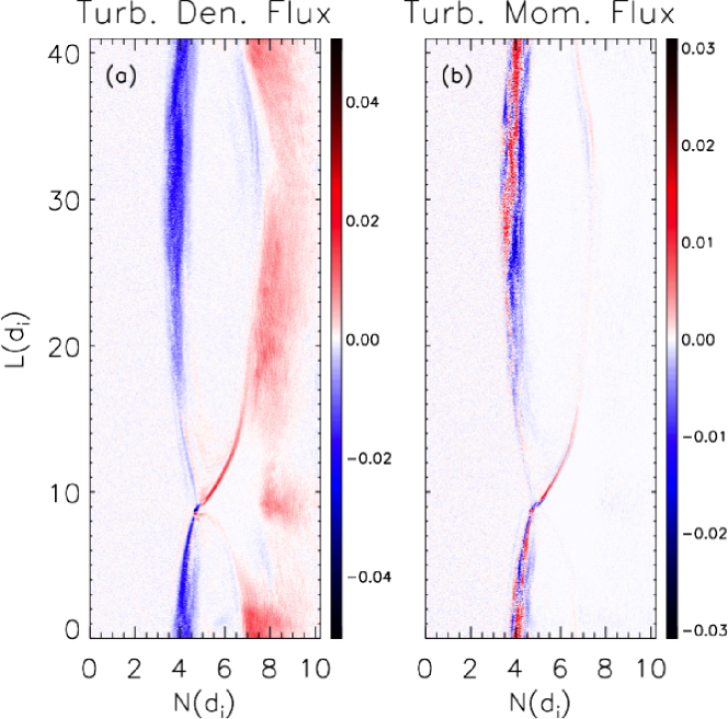
Figure 12: Images in the $L-N$ plane of (a): $\Gamma_{N,\perp}=\langle\delta n\delta V_{eN,\perp})\rangle$ and (b): $\langle\delta v_{N\perp}\delta(nv_{M})\rangle$ at $t=26$.

If the electron density can undergo diffusion across the magnetopause even when the electrons remain frozen-in, it is possible that the $M$ component of the electron momentum (current) can do so as well. In the case of an anti-parallel magnetic configuration the coupled diffusion problem has been completed Drake et al. (1981). In the context of the present simulations with a strong guide field, we are not interested in solving the full coupled diffusion equations but rather focus on the diffusion of the electron momentum in the $M$ direction. Consider the $M$ component of Ohm’s law and assume that the electrons are completely frozen-in and that the divergence of the electron pressure can be neglected. The $M$ component of the momentum equation becomes

$$\frac{\partial(nV_{M})}{\partial t}+\bm{\nabla\cdot}[\mathbf{v}(nV_{M})]=0,$$ (4)

which is simply the diffusion equation for the current $nV_{M}$. Once the equation is broken into laminar and fluctuating parts, the transport of momentum is given by the turbulent momentum flux

$$\langle\delta V_{N\perp}\delta(nV_{M})\rangle,$$ (5)

where we have retained only the the perpendicular transport of $nV_{M}$. The individual components of this equation are again shown in cuts along the $M$ direction in Figure 11b. The flux of the out-of-plane current in the $N$ direction normal to $\mathbf{B}$ is shown in Figure 12b. The flux is strong, particularly on the downstream magnetospheric separatrix and exhibits an asymmetry in the north-south direction due to the presence of the guide field. When normalized by the averaged out-of-plane current density, $\langle nv_{M}\rangle$, this flux is larger than the similarly normalized particle flux shown in Figure 12b. The frozen-in nature of the electrons is a natural consequence of the temporal and spatial scales associated with the turbulence. What is a surprise is that, despite this restriction, the turbulence still manages to transport momentum efficiently across the separatrix.

IV Discussion

The inclusion of the third dimension in numerical simulations of magnetopause reconnection permits the development of strong turbulence regardless of the presence of a guide field. In both cases the strong density gradient drives the development of a form of lower hybrid drift instability along the magnetic separatrices downstream from the X-line. In the guide field case magnetic shear is not effective in stabilizing the LHDI downstream of the X-line because the rotation of the magnetic field occurs over a scale size of the order of the width of the magnetic island while the gradient in the plasma density is highly localized across the magnetic separatrix. At late time there is a balance between the steepening of the gradient as the magnetic island expands into the low density magnetosphere and the turbulence associated with LHDI. Very near the X-line, unlike the anti-parallel case, LHDI is stabilized. Nevertheless, an electromagnetic instability develops with a wavelength that greatly exceeds that due to LHDI. Although the turbulence in all instances contributes to balancing the reconnection electric field, the overall reconnection rate is essentially unaffected.

An important issue related to the impact of turbulence driven by the LHDI at the magnetopause concerns the response of electrons to the fluctuations. Because the turbulence is low frequency compared to the electron gyrofrequency and because the $\bm{\nabla}B$ drift velocities of electrons are typically small compared with the phase speed of the wave, electrons are typically frozen-in to the fluctuations. This frozen-in behavior has been documented with the observations from the MMS mission Graham et al. (2019). Within linear theory electrons are therefore non-resonant and cannot undergo irreversible diffusion nor contribute to the average Ohm’s law describing large-scale reconnection. However, we have shown that the LHDI-driven turbulence reaches large enough amplitude for the electrons to undergo fluid-like turbulent diffusion Kleva and Drake (1984). In this regime the electrons experience a nonlinear resonant interaction with the fluctuations. This turbulent diffusion can drive transport of both the electron density $n$ and the out-of-plane current density $nV_{eM}$.

Reconnection in asymmetric configurations can be stabilized by the presence of diamagnetic drifts Swisdak et al. (2003, 2010); Phan et al. (2013), with complete stabilization occurring when the difference in $\beta=8\pi P/B^{2}$ between the asymptotic plasmas exceeds $\approx 2\tan{\theta/2}$, where $\theta$ is the shear angle between the reconnecting fields. In the configuration considered here, $\Delta\beta\approx 2.5$ and $2\tan{(\theta/2)}\approx 4.8$. Hence the reconnection is not strongly affected by diamagnetic drifts, which is in agreement with the reconnection rate of $\mathcal{O}(0.1)$ observed for the both the two-dimensional and three-dimensional simulations.

An important question is whether real mass-ratio simulations (here $m_{i}/m_{e}=100$) would give different results. Even with a realistic mass ratio, the LHDI will be strong in systems with scale lengths near the ion Larmor radius, which is characteristic of the boundary layers with strong $E_{N}$ at the magnetopause. The suppression of LHDI by magnetic shear and finite $\beta$ is weaker in asymmetric reconnection because the strongest density gradient and peak current $J_{eM}$, which drive the instability, are on the magnetosphere side of the X-line where $\beta$ is smaller. Comparisons of simulations of anti-parallel reconnection with $m_{i}/m_{e}=100$ and $m_{i}/m_{e}=400$ found qualitative similarities, although the amplitude of the LHDI and its extent in the $N$ direction were greater in the latter case Price et al. (2017). We anticipate similar results will hold for the guide-field case along the separatrices away from the X-line. However, the scaling near the X-line is less certain, particularly for the inertial terms that make a significant contribution to the generalized Ohm’s law in Figure 7(b).

Appendix A Averaged Generalized Ohm’s Law

In order to derive the various contributions arising from turbulent fluctuations, begin with the momentum equation for the electron fluid

$$en\mathbf{E}=-mn\frac{d\mathbf{v}}{dt}-\bm{\nabla\cdot}\mathbb{P}-en(\mathbf{v}\bm{\times}\mathbf{B})/c$$ (6)

where $m$, $n$, $\mathbf{v}$, and $\mathbb{P}$ are the electron mass, density, velocity, and pressure tensor and $d/dt$ represents the total (convective) derivative. Next, average over the $M$ direction and decompose every quantity into a mean and fluctuating component, i.e., $n=\langle n\rangle+\delta n$. Note that products of quantities produce two potentially non-zero terms, $\langle AB\rangle=\langle A\rangle\langle B\rangle+\langle\delta A\delta B\rangle$ and triple products (e.g., $n\mathbf{v}\bm{\times}\mathbf{B}$) produce five, including one average of three fluctuating terms. Previous applications of this approach Price et al. (2016, 2017); Le et al. (2017) have combined the number density and fluid velocity in the final term of equation 6 into a single current density term $\mathbf{J}$. Here, in contrast, we separate $\mathbf{J}$ into its constituent parts in the Lorentz force term – although not the terms proportional to the mass $m$ – in order to explore the degree to which electrons remain frozen to the magnetic field. The final result is

$$\begin{split}e\langle n\rangle\langle E_{M}\rangle=&\frac{e}{c}\Bigl{(}\langle n\rangle\langle v_{L}\rangle\langle B_{N}\rangle-\langle n\rangle\langle v_{N}\rangle\langle B_{L}\rangle\Bigr{)}\\ &-\frac{\partial}{\partial L}\langle P_{LM}\rangle-\frac{\partial}{\partial N}\langle P_{NM}\rangle\\ &+\frac{m}{e}\left(\frac{\partial}{\partial L}\langle v_{L}\rangle\langle J_{M}\rangle+\frac{\partial}{\partial N}\langle v_{N}\rangle\langle J_{M}\rangle+\frac{\partial}{\partial t}\langle J_{M}\rangle\right)\\ &-e\langle\delta n\delta E_{M}\rangle\\ &+\frac{m}{e}\left(\frac{\partial}{\partial L}\langle\delta J_{M}\delta v_{L}\rangle+\frac{\partial}{\partial N}\langle\delta J_{M}\delta v_{N}\rangle\right)\\ &+\frac{e}{c}\Bigl{(}\langle n\rangle\langle\delta v_{L}\delta B_{N}\rangle-\langle n\rangle\langle\delta v_{N}\delta B_{L}\rangle\\ &\qquad+\langle B_{N}\rangle\langle\delta n\delta v_{L}\rangle-\langle B_{L}\rangle\langle\delta n\delta v_{N}\rangle\\ &\qquad+\langle v_{L}\rangle\langle\delta n\delta B_{N}\rangle-\langle v_{N}\rangle\langle\delta n\delta B_{L}\rangle\\ &\qquad+\langle\delta n\delta v_{L}\delta B_{N}\rangle-\langle\delta n\delta v_{N}\delta B_{L}\rangle\Bigr{)}\end{split}$$ (7)