Liquid velocity fluctuations and energy spectra in three-dimensional buoyancy driven bubbly flows

Abstract

We present a direct numerical simulation (DNS) study of pseudo-turbulence in buoyancy driven bubbly flows for a range of Reynolds (Re) and Atwood (At) numbers. We study the probability distribution function of the horizontal and vertical liquid velocity fluctuations and find them to be in quantitative agreement with the experiments. The energy spectrum shows the $k^{-3}$ scaling at high Re and becomes steeper on reducing the Re. To investigate the spectral transfers in the flow, we derive the scale-by-scale energy budget equation. Our analysis shows that, for scales smaller than the bubble diameter, the net production because of the surface tension and the kinetic energy flux balances viscous dissipation to give the $k^{-3}$ scaling of the energy spectrum for both low and high At.

1 Introduction

Bubble laden flow appears in a variety of natural (Clift et al., 1978; Gonnermann & Manga, 2007) and industrial (Deckwer, 1992) processes. Presence of bubbles dramatically alters the transport properties of a flow (Mudde, 2005; Ceccio, 2010; Biferale et al., 2012; Pandit et al., 2017; Risso, 2018; Elghobashi, 2019; Mathai et al., 2019). A single bubble of diameter $d$, because of buoyancy, rises under gravity. Its trajectory and the wake flow depend on the density and viscosity contrast with the ambient fluid, and the surface tension (Clift et al., 1978; Bhaga & Weber, 1981; Tripathi et al., 2015). A suspension of such bubbles at moderate volume fractions generates complex spatiotemporal flow patterns that are often referred to as pseudo-turbulence or bubble-induced agitation (Mudde, 2005; Risso, 2018).

Experiments have made significant progress in characterizing velocity fluctuations of the fluid phase in pseudo-turbulence. A key observation is the robust power-law scaling in the energy spectrum with an exponent of $-3$ either in frequency $f$ or the wave-number $k$ space (Mercado et al., 2010; Riboux et al., 2010; Mendez-Diaz et al., 2013). The scaling range, however, remains controversial. Riboux et al. (2010) investigated turbulence in the wake of a bubble swarm and found the $k^{-3}$ scaling for length scales larger than the bubble diameter $d$ (i.e., $k<2\pi/d$), whereas Mercado et al. (2010); Prakash et al. (2016) observed this scaling for scales smaller than $d$ in a steady state bubble suspension. Experiments on bouyancy driven bubbly flows in presence of grid-turbulence (Lance & Bataille, 1991; Prakash et al., 2016; Alméras et al., 2017) observe Kolmogorov scaling for scales larger than the bubble diameter and smaller than the forcing scale and a much steeper $k^{-3}$ scaling for scales smaller than the bubble diameter and larger than the dissipation scale. Lance & Bataille (1991) argued that, assuming production because of wakes to be local in spectral space, balance of production with viscous dissipation leads to the observed $k^{-3}$ scaling.

Fully resolved numerical simulations of three-dimensional (3D) bubbly flows for a range of Reynolds number $O(10)<\mbox{Re}<O(10^{3})$ (Roghair et al., 2011; Bunner & Tryggvason, 2002b, a) found the $k^{-3}$ scaling for length scales smaller than $d$ ($k>2\pi/d$) and attributed it to the balance between viscous dissipation and the energy production by the wakes (Lance & Bataille, 1991).

Two mechanisms proposed to explain the observed scaling behavior in experiments are: $(i)$ superposition of velocity fluctuations generated in the vicinity of the bubbles (Risso, 2011), and $(ii)$ at high Re, the instabilities in the flow through bubble swarm (Lance & Bataille, 1991; Mudde, 2005; Risso, 2018). In an experiment or a simulation, it is difficult to disentangle these two mechanisms.

In classical turbulence, a constant flux of energy is maintained between the injection and dissipation scales (Frisch, 1997; Pandit et al., 2009; Boffetta & Ecke, 2012). In pseudo-turbulence, on the other hand, it is not clear how the energy injected because of buoyancy is transferred between different scales. In particular, the following key questions remain unanswered: $(i)$ How do liquid velocity fluctuations and the pseudo-turbulence spectrum depend on the Reynolds number (Re)? $(ii)$ What is the energy budget and the dominant balances? $(iii)$ Is there an energy cascade (a non-zero energy flux)?

In this paper, we address all of the above questions for experimentally relevant Reynolds (Re) and Atwood (At) numbers. We first investigate the dynamics of an isolated bubble and show that the wake flow behind the bubble is in agreement with earlier experiments and simulations. Next for a bubbly suspension we show that the the liquid velocity fluctuations are in quantitative agreement with the experiments of Riboux et al. (2010) and the bubble velocity fluctuations are in quantitative agreement with the simulations of Roghair et al. (2011). We then proceed to derive the scale-by-scale energy budget equation and investigate the dominant balances for different Re and At. We find that for scales smaller than the bubble diameter, viscous dissipation balances net nonlinear transfer of energy because of advection and the surface tension to give $k^{-3}$ psuedo-turbulence spectrum. Intriguingly, the dominant balances are robust and do not depend on the density contrast (At).

2 Model and Numerical Details

We study the dynamics of bubbly flow by using Navier-Stokes (NS) equations with a surface tension force because of bubbles

$$\rho D_{t}\bm{u} = \nabla\bm{\cdot}[2\mu{\cal S}]-\nabla p+{\bm{F}}^{\sigma}+{\bm{F}}^{g},$$ (1a)

$$\nabla\bm{\cdot}\bm{u} = 0.$$ (1b)

Here, $D_{t}=\partial_{t}+(\bm{u}\cdot\nabla)$ is the material derivative, ${\bm{u}}=(u_{x},u_{y},u_{z})$ is the hydrodynamic velocity, $p$ is the pressure, ${\cal S}\equiv(\nabla{\bm{u}}+\nabla{\bm{u}}^{T})/2$ is the rate of deformation tensor, $\rho\equiv\rho_{f}c+\rho_{b}(1-c)$ is the density, $\mu\equiv\mu_{f}c+\mu_{b}(1-c)$ is the viscosity, $\rho_{f}$ ($\rho_{b}$) is the fluid (bubble) density, and $\mu_{b}$ ($\mu_{f}$) is the bubble (fluid) viscosity. The value of the indicator function $c$ is equal to zero in the bubble phase and unity in the fluid phase. The surface tension force is $\bm{F}^{\sigma}\equiv\sigma\kappa\hat{\bm{n}}$, where $\sigma$ is the coefficient of surface tension, $\kappa$ is the curvature, and $\hat{\bm{n}}$ is the normal to the bubble interface. ${\bm{F}}^{g}\equiv[\rho_{a}-\rho]g\hat{\bm{z}}$ is the buoyancy force, where $g$ is the accelaration due to gravity, and $\rho_{a}\equiv[\int\rho(c)d{\bm{x}}]/L^{3}$ is the average density. For small Atwood numbers, we employ Boussinesq approximation whereby, $\rho$ in the left-hand-side of Eq. (1a) is replaced by the average density $\rho_{a}$.

We solve the Boussinesq approximated NS using a pseudo-spectral method (Canuto et al., 2012) coupled to a front-tracking algorithm (Tryggvason et al., 2001; Aniszewski et al., 2019) for bubble dynamics. Time marching is done using a scond-order Adams-Bashforth scheme. For the non-Boussinesq NS, we use the open source finite-volume-front-tracking solver PARIS (Aniszewski et al., 2019).

We use a cubic periodic box of volume $L^{3}$ and discretize it with $N^{3}$ collocation points. We initialize the velocity field ${\bm{u}}=0$ and place the centers of $N_{b}$ bubbles at random locations such that no two bubbles overlap. The Reynolds number Re, the Bond number Bo, and the bubble volume fraction $\phi\equiv[\int(1-c)d{\bm{x}}]/L^{3}$ that we use (see table 1) are comparable to the experiments (Mendez-Diaz et al., 2013; Riboux et al., 2010).

runs	$L$	$N$	$N_{b}$	$d$	$g$	$\mu_{f}$	$\phi\%$	Re	At	Bo	$\epsilon_{\mu}$	$\epsilon_{w}$	$\epsilon_{\mu,f}$	$\epsilon_{inj}$
$\tt{R1}$	$256$	$512$	$60$	$24$	$1.0$	$0.32$	$2.6$	$104$	$0.04$	$1.8$	$3.6\cdot 10^{-3}$	$2.8\cdot 10^{-3}$	$2.0\cdot 10^{-3}$	$3.5\cdot 10^{-3}$
$\tt{R2}$	$256$	$512$	$60$	$24$	$1.0$	$0.20$	$2.6$	$166$	$0.04$	$1.0$	$4.3\cdot 10^{-3}$	$2.8\cdot 10^{-3}$	$2.6\cdot 10^{-3}$	$4.3\cdot 10^{-3}$
$\tt{R3}$	$128$	$432$	$10$	$22$	$8.75$	$0.42$	$2.6$	$206$	$0.04$	$2.1$	$9.5\cdot 10^{-2}$	$7.1\cdot 10^{-2}$	$6.7\cdot 10^{-2}$	$9.4\cdot 10^{-2}$
$\tt{R4}$	$128$	$432$	$10$	$22$	$10.5$	$0.32$	$2.6$	$296$	0.04	$1.9$	$1.3\cdot 10^{-1}$	$9.4\cdot 10^{-2}$	$9.6\cdot 10^{-2}$	$1.3\cdot 10^{-1}$
$\tt{R5}$	$256$	$256$	$40$	$24$	$0.1$	$0.32$	$1.7$	$113$	$0.90$	$2.0$	$3.2\cdot 10^{-3}$	$2.4\cdot 10^{-3}$	$1.8\cdot 10^{-3}$	$3.0\cdot 10^{-3}$
$\tt{R6}$	$256$	$256$	$40$	$24$	$1.0$	$0.32$	$1.7$	$345$	$0.80$	$2.4$	$8.1\cdot 10^{-2}$	$6.9\cdot 10^{-2}$	$5.4\cdot 10^{-2}$	$8.4\cdot 10^{-2}$
$\tt{R7}$	$256$	$256$	$40$	$24$	$1.0$	$0.32$	$1.7$	$358$	$0.90$	$1.9$	$1.0\cdot 10^{-1}$	$7.7\cdot 10^{-2}$	$6.2\cdot 10^{-2}$	$1.0\cdot 10^{-1}$

Table 1: Table of parameters used in our DNS. Here, $\delta\rho\equiv\rho_{f}-\rho_{b}$ is the density difference, $\mbox{Re}\equiv\sqrt{\rho_{f}\delta\rho gd^{3}}/\mu_{f}$ is the Reynolds number, $\mbox{Bo}\equiv\delta\rho gd^{2}/\sigma$ is the Bond number, $\mbox{At}=\delta\rho/(\rho_{f}+\rho_{b})$ is the Atwood number, $\epsilon_{w}\equiv\phi(\delta\rho gd/\rho_{f})^{3/2}/d$ is the estimate of the energy dissipation rate because of the bubble wakes (Lance & Bataille (1991)), and $\epsilon_{\mu,f}$ is the energy dissipation rate in the fluid phase. We fix the value of the fluid density $\rho_{f}=1$ and assume same viscosity for the fluid and the bubble phase $\mu_{f}/\mu_{b}=1$.

3 Results

In subsequent sections, we investigate statistical properties of stationary pseudo-turbulence generated in buoyancy driven bubbly flows. Table 1 lists the parameters used in our simulations. Our parameters are chosen such that the Reynolds number, Bond number, and the volume fraction are comparable to those used in earlier experiments (Riboux et al., 2010; Mendez-Diaz et al., 2013; Risso, 2018). We conduct simulations at both low and high-At numbers to investigate role of density difference on the statistics of pseudo-turbulence. The rest of the paper is organized as follows. In §§ 3.1 we study the trajectory of an isolated bubbles and, consistent with the experiments, show that the bubble shape is ellipsoidal. In §§ 3.2-3.3 we investigate the total kinetic energy budget and the fluid and bubble centre-of-mass velocity fluctuations and make quantitative comparison with the experiments. Finally, in §§ 3.4 we study the kinetic energy spectrum and scale-by-scale energy budget analysis. We present our conclusions in § 4.

3.1 Single bubble dynamics

In this section we study the dynamics an initially spherical bubble as it rises because of buoyancy. The seminal work of Bhaga & Weber (1981) characterized the shape and trajectory of an isolated bubble in terms of Reynolds and Bond number. Experiments on turbulent bubbly flows (Lance & Bataille, 1991; Prakash et al., 2016) observe ellipsoidal bubbles. In the following, we characterize the dynamics of an isolated bubble for the parameters used in our simulations.

To avoid the interaction of the bubble with its own wake, we use a vertically elongated cuboidal domain of dimension $5d\times 5d\times 21d$. After the bubble rise velocity attains steady-state, figure 1(a-c) shows the bubble shape and the vertical component of the vorticity $\omega_{z}=(\nabla\times{\bm{u}})\cdot\hat{z}$. For $\mbox{Re}=104$ and $\mbox{At}=0.04$ (run R1), the bubble shape is oblate ellipsoid and it rises in a rectilinear trajectory. On increasing the $\mbox{Re}=295$ (run R4), the bubble pulsates while rising and sheds varicose vortices similar to Pivello et al. (2014). Finally, for high $\mbox{At}=0.80$ and $\mbox{Re}=345$ (run R6), similar to region III of Tripathi et al. (2015), we find that the bubble shape is oblate ellipsoid and it follows a zigzag trajectory.

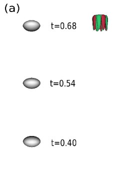
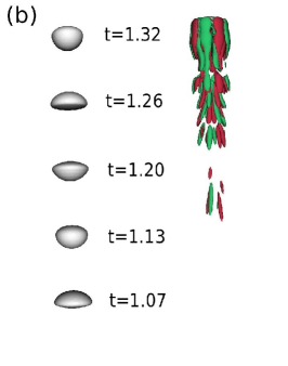
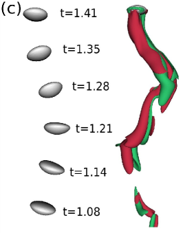
Figure 1: Bubble positions at different times (in units of $\tau_{s}$) and the z-component of the vorticity ($\omega_{z}=\partial_{x}u_{y}-\partial_{y}u_{x}$) for the case of single bubble rising under gravity. The non-dimensional parameters in representative cases are taken same as run R1 in panel (a), run R4 in panel (b), and run R6 in panel (c). Green region corresponds to $\omega_{z}<0$, whereas red region corresponds to $\omega_{z}>0$. We plot iso-contours corresponding to $|\omega_{z}|=\pm 10^{-3}$ in (a), $|\omega_{z}|=\pm 10^{-2}$ in (b), and $|\omega_{z}|=\pm 10^{-1}$ in (c).

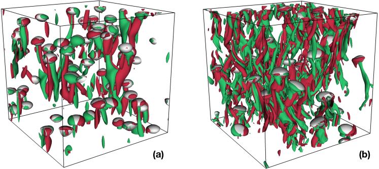
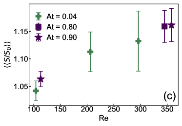
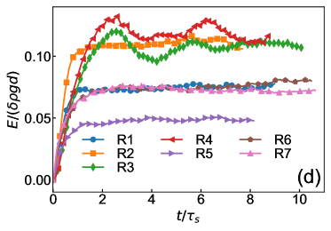
Figure 2: Representative steady-state snapshot of the bubbles overlayed on the iso-contour plots of the $z$-component of the vorticity field $\omega_{z}\equiv[\nabla\times{\bm{u}}]\cdot\hat{\bm{z}}$ for $\mbox{Re}=104$, $\mbox{At}=0.04$ (a) and for $\mbox{Re}=345$, $\mbox{At}=0.78$ (b). Regions with $\omega_{z}=2\sigma_{\omega}(-2\sigma_{\omega})$ are shown in red (green), where $\sigma_{\omega}$ is the standard deviation of $\omega_{z}$. As expected, bubble-wake interactions becomes more intense on increasing Re. (c) Re versus average bubble deformation $\langle\langle S(t)/S(0)\rangle\rangle$ for low $\mbox{At}=0.04$ and high At numbers, and (d) Kinetic energy evolution for the runs given in table 1.

3.2 Bubble suspension and kinetic energy budget

The plots in figure 2(a,b) show the representative steady state iso-vorticity contours of the $z$-component of the vorticity along with the bubble interface position for our bubbly flow configurations. As expected from our isolated bubble study in the previous section, we observe rising ellipsoidal bubbles and their wakes which interact to generate pseudo-turbulence. The individual bubbles in the suspension show shape undulations which are similar to their isolated bubble counterparts [see movies available in the supplementary material]. Furthermore, for comparable $\mbox{Bo}\approx 2$, the average bubble deformation $\langle\langle S(t)/S(0)\rangle\rangle$ increases with increasing Re [figure 2(c)]. Here, $\langle\langle\cdot\rangle\rangle$ denote temporal averaging over bubble trajectories in the statistically steady state, $S(t)$ is the surface area of the bubble, and $S(0)=\pi d^{2}$.

The time evolution of the kinetic energy $E=\langle\rho u^{2}/2\rangle$ for runs R1 - R7 is shown in figure 2(d). A statistically steady state is attained around $t\approx 2.5\tau_{s}$, where $\tau_{s}=L/\sqrt{\delta\rho gd/\rho_{f}}$ is the approximate time taken by an isolated bubble to traverse the entire domain. Using Eq. (1a), we obtain the total kinetic energy $E$ balance equation as

$$\partial_{t}\underbrace{\langle\frac{\rho{\bm{u}}^{2}}{2}\rangle}_{E}=-\underbrace{2\langle\mu(c)\mathcal{S}:\mathcal{S}\rangle}_{\epsilon_{\mu}}+\underbrace{\langle[\rho_{a}-\rho(c)]u_{y}g\rangle}_{\epsilon_{inj}}+\underbrace{\langle\bm{F}^{\sigma}\cdot\bm{u}\rangle}_{\epsilon_{\sigma}},$$ (2)

where, $\langle\cdot\rangle$ represents spatial averaging. In steady state, the energy injected by buoyancy $\epsilon_{inj}$ is balanced by viscous dissipation $\epsilon_{\mu}$. The energy injected by buoyancy $\epsilon_{inj}\approx(\rho_{f}-\rho_{b})\phi g\langle U\rangle$ where $\langle U\rangle$ is the average bubble rise velocity. Note that $\epsilon_{\sigma}=-\partial_{t}\int\sigma ds$ (Joseph, 1976), where $ds$ is the bubble surface element, and its contribution is zero in the steady-state. The excellent agreement between steady state values of $\epsilon_{\mu}$ and $\epsilon_{inj}$ is evident from table 1.

Lance & Bataille (1991) argued that the energy injected by the buoyancy is dissipated in the wakes on the bubble. The energy dissipation in the wakes can be estimated as $\epsilon_{w}=C_{d}\phi((\delta\rho/\rho_{f})gd)^{3/2}/d$, where $C_{d}$ is the drag coefficient. Assuming $C_{d}=O(1)$, we find that $\epsilon_{w}$ is indeed comparable to the viscous dissipation in the fluid phase $\epsilon_{\mu,f}$ (see table 1).

3.3 Probability distribution function of the fluid and bubble velocity fluctuations

In figure 3(a,b) we plot the probability distribution function (p.d.f.) of the fluid velocity fluctuations ${\bm{u}}^{f}\equiv{\bm{u}}[c=1]$. Both the horizontal and vertical velocity p.d.f.’s are in quantitative agreement with the experimental data of Riboux et al. (2010) and Risso (2018). The p.d.f. of the velocity fluctuations of the horizontal velocity components are symmetric about origin and have stretched exponential tails, whereas the vertical velocity fluctuations are positively skewed (Riboux et al., 2010; Alméras et al., 2017; Prakash et al., 2016). Our results are consistent with the recently proposed stochastic model of Risso (2016) which suggests that the potential flow disturbance around bubbles, bubble wakes, and the turbulent agitation because of flow instabilities together lead to the observed velocity distributions. We believe that the deviation in the tail of the distributions arises because of the differences in the wake flow for different Re and At (see figure 1). Note that positive skewness in the vertical velocity has also been observed in thermal convection with bubbles (Biferale et al., 2012).

By tracking the individual bubble trajectories we obtain their center-of-mass velocity ${\bm{u}}^{b}$. In agreement with the earlier simulations of Roghair et al. (2011), the p.d.f.’s of the bubble velocity fluctuation are Gaussian (see figure 4). The departure in the tail of the distribution is most probably because of the presence of large scale structures observed in experiments that are absent in simulations with periodic boundaries (Roghair et al., 2011).

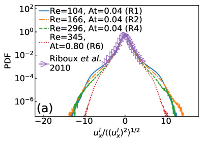
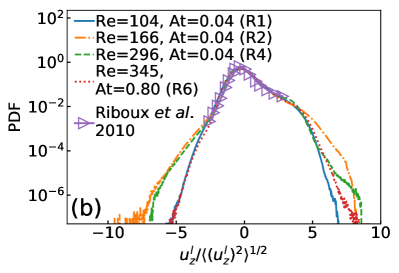
Figure 3: The probability distribution function of the (a) horizontal component (b) vertical component of the liquid velocity fluctuations for runs given in table 1. The p.d.f. obtained from our DNS are in excellent agreement with the experimental data of Riboux et al. (2010) [Data extracted using enguage https://markummitchell.github.io/engauge-digitizer/].

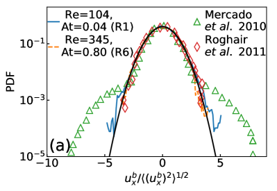
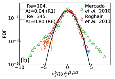
Figure 4: The probability distribution function of (a) the horizontal and (b) the vertical component of the bubbles velocity fluctuations for runs R1 and R6 (see table 1). The experimental data of Mercado et al. (2010) and numerical results of Roghair et al. (2011) is also shown for comparison. The black continuous line represents a Gaussian distribution.

3.4 Energy spectra and scale-by-scale budget

In the following, we study the energy spectrum

$$\displaystyle E^{uu}_{k} \equiv \sum_{k-1/2<m<k+1/2}|\hat{\bm{u}}_{m}|^{2},$$

the co-spectrum

$$\displaystyle E^{\rho uu}_{k} \equiv \sum_{k-1/2<m<k+1/2}\Re[\hat{(\rho{\bm{u}})}_{-m}\hat{\bm{u}}_{m}]\equiv d\mathscr{E}/dk,$$

and the scale-by-scale energy budget. Our derivation of the energy budget is similar to (Frisch, 1997; Pope, 2012) and does not require the flow to be homogeneous and isotropic. For a general field $f({\bm{x}})$, we define a corresponding coarse-grained field (Frisch, 1997) $f^{<}_{k}({\bm{x}})\equiv\sum_{m\leq k}f_{\bm{m}}\exp(i{\bm{m}}\cdot{\bm{x}})$ with the filtering length scale $\ell=2\pi/k$. Using the above definitions in Eq. (1a), we get the energy budget equation

$$\partial_{t}\mathscr{E}_{k}+\Pi_{k}+\mathscr{F}^{\sigma}_{k}=\mathscr{P}_{k}-\mathscr{D}_{k}+\mathscr{F}^{g}_{k}.$$ (3)

Here, $2\mathscr{E}_{k}=\langle\bm{u}^{<}_{k}\cdot(\rho\bm{u})^{<}_{k}\rangle$ is the cumulative energy up to wave-number $k$, $2\Pi_{k}=\langle(\rho\bm{u})^{<}_{k}\bm{\cdot}(\bm{u}\bm{\cdot}\nabla\bm{u})^{<}_{k}\rangle+\langle\bm{u}^{<}_{k}\bm{\cdot}(\bm{u}\bm{\cdot}\nabla\rho\bm{u})^{<}_{k}\rangle$ is the energy flux through wave-number $k$, $2\mathscr{D}_{k}=-[\langle(\rho\bm{u})^{<}_{k}\bm{\cdot}\left(\nabla\bm{\cdot}[2\mu{\cal S}]/\rho\right)^{<}_{k}\rangle+\langle\bm{u}^{<}_{k}\bm{\cdot}(\nabla\bm{\cdot}[2\mu{\cal S}])^{<}_{k}\rangle]$ is the cumulative energy dissipated upto $k$, $2\mathscr{F}^{\sigma}_{k}=-[\langle(\rho\bm{u})^{<}_{k}\bm{\cdot}\left(\bm{F}^{\sigma}/\rho\right)^{<}_{k}\rangle+\langle\bm{u}^{<}_{k}\bm{\cdot}(\bm{F}^{\sigma})^{<}_{k}\rangle]$ is the cumulative energy transferred from the bubble surface tension to the fluid upto $k$, $2\mathscr{F}^{g}_{k}=\langle(\rho\bm{u})^{<}_{k}\bm{\cdot}\left(\bm{F}^{g}/\rho\right)^{<}_{k}\rangle+\langle\bm{u}^{<}_{k}\bm{\cdot}(\bm{F}^{g})^{<}_{k}\rangle$ is cumulative energy injected by buoyancy upto $k$. In crucial departure from the uniform density flows, we find a non-zero cumulative pressure contribution $2\mathscr{P}_{k}=\langle(\rho\bm{u})^{<}_{k}\bm{\cdot}\left({\nabla p}/{\rho}\right)^{<}_{k}\rangle$.

In the Boussinesq regime (small At), the individual terms in the scale-by-scale budget simplify to their uniform density analogues: $\mathscr{E}_{k}=\rho_{a}\langle\bm{u}^{<}_{k}\cdot\bm{u}^{<}_{k}\rangle/2$, $\Pi_{k}=\rho_{a}\langle\bm{u}^{<}_{k}\bm{\cdot}(\bm{u\cdot}\nabla\bm{u})^{<}_{k}\rangle$, $\mathscr{D}_{k}=-\mu\langle|\nabla{\bm{u}}_{k}^{<}|^{2}\rangle$, $\mathscr{F}^{\sigma}_{k}=-\langle\bm{u}^{<}_{k}\bm{\cdot}(\bm{F}^{\sigma})^{<}_{k}\rangle$, $\mathscr{F}^{g}_{k}=\langle\bm{u}^{<}_{k}\bm{\cdot}(\bm{F}^{g})^{<}_{k}\rangle$, and $\mathscr{P}_{k}=0$.

3.4.1 Low At (runs $\tt{R1}-\tt{R4}$)

We first discuss the results for the Boussinesq regime (low At). For scales smaller than the bubble diameter ($k>k_{d}$), the energy spectrum (figure 5(a)) shows a power-law behavior $E(k)\sim k^{-\beta}$ for different Re. The exponent $\beta=4$ for $\mbox{Re}=104$, it decreases on increasing the Re and becomes close to $\beta=3$ for the largest $\mbox{Re}=296$.

We now investigate the dominant balances using the scale-by-scale energy budget analysis. In the statistically steady-state $\partial_{t}{\mathscr{E}}_{k}=0$, and $\Pi_{k}+\mathscr{F}^{\sigma}_{k}=-\mathscr{D}_{k}+\mathscr{F}^{g}_{k}$ (note that $\mathscr{P}_{k}=0$ for low At). In figure 5(b) and figure 5(c) we plot different contributions to the cumulative energy budget for $\mbox{Re}\approx 104$ and $\mbox{Re}\approx 300$ and make the following observations:

1. Cumulative energy injected by buoyancy ${\mathscr{F}}_{k}^{\sigma}$ saturates around $k\approx k_{d}$. Thus buoyancy injects energy at scales comparable to and larger than the bubble diameter.

2. Energy flux $\Pi_{k}>0$ around $k\approx k_{d}$ and it vanishes for $k\gg k_{d}$.

3. Especially for scales smaller than the bubble diameter, the cumulative energy transfer from the bubble surface tension to the velocity is the dominant energy transfer mechanism.

4. Consistent with the earlier predictions (Riboux et al., 2010), for our highest $\mbox{Re}=300$ simulation provides a direct evidence that the balance of total production $d(\Pi_{k}+{\mathscr{F}}_{k}^{\sigma})/dk\sim k^{-1}$ with viscous dissipation [$d{\mathscr{D}}_{k}/dk=\nu k^{2}E(k)$] gives the psuedo-turbulence spectra $E(k)\sim k^{-3}$ (Riboux et al., 2010; Roghair et al., 2011; Mercado et al., 2010).

Our scale-by-scale analysis, therefore, suggests the following mechanism of pseudo-turbulence. Buoyancy injects energy at scales comparable to and larger to the bubble size. A part of the energy injected by buoyancy is absorbed in stretching and deformation of the bubbles and another fraction is transferred via wakes to scales comparable to bubble diameter. Similar to polymers in turbulent flows Perlekar et al. (2006, 2010); Valente et al. (2014), the relaxation of the bubbles leads to injection of energy at scales smaller than the bubble diameter.

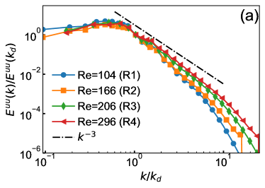
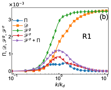
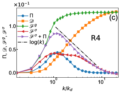
Figure 5: (a) Log-log plot of energy spectra $E^{uu}_{k}$ versus $k/k_{d}$ for our high Re low At runs R1 - R4. Dashed dotted line indicates the $k^{-3}$ scaling. Cumulative contribution of viscous dissipation $\mathscr{D}_{k}$, energy injected because of buoyancy $\mathscr{F}^{g}_{k}$ and the surface tension contribution $\mathscr{F}^{\sigma}_{k}$ versus $k/k_{d}$ for (b) run $\tt{R1}$ and (c) run R4. Note that, for $k>k_{d}$, the balance between $d\mathscr{F}_{k}^{\sigma}/dk$ and $d\mathscr{D}_{k}/dk$ is more prominent in panel (c) compared to (b).

3.4.2 High At (runs $\tt{R5-R7}$)

Similar to earlier section, here also the energy spectrum and the co-spectrum shows a $k^{-3}$ (figure 6(a)). However, because of density variations the scale-by-scale energy budget becomes more complex. Now, in the statistically steady state

$\Pi_{k}+\mathscr{F}^{\sigma}_{k}=\mathscr{P}_{k}-\mathscr{D}_{k}+\mathscr{F}^{g}_{k}$.

In (figure 6(b)) we plot the scale-by-scale energy budget for our high At run ${\tt R5}$. We find that the cumulative energy injected by buoyancy and the pressure contribution ${\mathscr{F}}_{k}^{g}+\mathscr{P}_{k}$ reaches a peak around $k\approx k_{d}$ and then decrease mildly to $\epsilon_{inj}$. Similar to the low At case, we find a non-zero energy flux for $k\approx k_{d}$ and a dominant surface-tension contribution to the energy budget for $k\gg k_{d}$. Finally, similar to last section, for $k>k_{d}$ the net production $d(\Pi+\mathscr{F}^{\sigma})/dk\sim k^{-1}$ balances viscous dissipation $\nu k^{2}E(k)$ to give $E(k)\sim k^{-3}$.

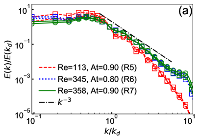
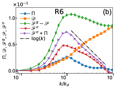
Figure 6: (a) Log-log plot of energy spectra ($\bigcirc$) $E^{uu}_{k}$ and co-spectrum ($\square$) $E^{\rho uu}_{k}$versus $k/k_{d}$ for our high Re high At runs R5 - R7. Dashed dotted line indicates the $k^{-3}$ scaling. (b) Cumulative contribution of the viscous dissipation $\mathscr{D}_{k}$, the contribution due to buoyancy and pressure $\mathscr{F}_{k}^{g}-\mathscr{P}_{k}$, the energy flux $\mathcal{\Pi}_{k}$ and the surface tension contribution $\mathscr{F}_{k}^{\sigma}$ versus $k/k_{d}$ for run ${\tt R6}$.

4 Conclusion

To conclude, we have investigated the statistical properties of velocity fluctuations in psuedo-turbulence generated by buoyancy driven bubbly flows. The Re that we have explored are consistent with the $\mbox{Re}\sim[300-1000]$ used in the experiments (Riboux et al., 2010; Prakash et al., 2016; Mendez-Diaz et al., 2013). Our numerical simulations show that the shape of the p.d.f. of the velocity fluctuations is consistent with experiments over a wide range of Re and At numbers. For large Re and for low as well as high At, the energy spectrum shows a $k^{-3}$ scaling but it becomes steeper on reducing the Re. We observe a non-zero positive energy flux for scales comparable to the bubble diameter. Our scale-by-scale energy budget validates the theoretical prediction that the net production balances viscous dissipation to give $E(k)\sim k^{-3}$.

5 Acknowledgments

We thank D. Mitra and S. Banerjee for discussions. This work was supported by research grant No. ECR/2018/001135 from SERB, DST (India).

References

- Alméras et al. (2017) Alméras, E., Mathai, V., Lohse, D. & Sun, C. 2017 Experimental investigation of the turbulence induced by a bubble swarm rising within incident turbulence. J. Fluid Mech. 825, 1091–-1112.
- Aniszewski et al. (2019) Aniszewski, W., Arrufat, T., Crialesi-Esposito, M., Dabiri, S., Fuster, D., Ling, Y., Lu, J, Malan, L., Pal, S., Scardovelli, R., Tryggvason, G., Yecko, P. & Zaleski, S. 2019 PArallel, Robust, Interface Simulator (PARIS). hal–02112617.
- Bhaga & Weber (1981) Bhaga, D. & Weber, M. E. 1981 Bubbles in viscous liquids: shapes, wakes and velocities. J. Fluid Mech. 105, 61–85.
- Biferale et al. (2012) Biferale, L., Perlekar, P., Sbragaglia, M. & Toschi, F. 2012 Convection in multiphase fluid flows using lattice boltzmann methods. Phys. Rev. Lett. 108, 104502.
- Boffetta & Ecke (2012) Boffetta, G. & Ecke, R. E. 2012 Two-dimensional turbulence. Annu. Rev. Fluid Mech. 44 (1), 427–451.
- Bunner & Tryggvason (2002a) Bunner, B. & Tryggvason, G. 2002a Dynamics of homogeneous bubbly flows part 1. rise velocity and microstructure of the bubbles. Journal of Fluid Mechanics 466, 17–52.
- Bunner & Tryggvason (2002b) Bunner, B. & Tryggvason, G. 2002b Dynamics of homogeneous bubbly flows part 2. velocity fluctuations. J. Fluid Mech. 466, 53 – 84.
- Canuto et al. (2012) Canuto, C., Hussaini, M. Y., Quarteroni, A. M. & Zang, T. A. 2012 Spectral Methods in Fluid Dynamics. Springer-Verlag.
- Ceccio (2010) Ceccio, S. L. 2010 Friction drag reduction of external flows with bubble and gas injection. Annu. Rev. Fluid Mech. 42, 183.
- Clift et al. (1978) Clift, R., Grace, J. R. & Weber, M. E. 1978 Bubbles, drops and particles. Academic Press, New York.
- Deckwer (1992) Deckwer, W.-D. 1992 Bubbles Column reactors. Wiley.
- Elghobashi (2019) Elghobashi, S. 2019 Direct numerical simulation of turbulent flows laden with droplets or bubbles. Annu. Rev. Fluid Mech. 51, 217–244.
- Frisch (1997) Frisch, U. 1997 Turbulence, A Legacy of A. N. Kolmogorov. Cambridge University Press.
- Gonnermann & Manga (2007) Gonnermann, H. M. & Manga, M. 2007 The fluid mechanics inside a volcano. Annu. Rev. Fluid Mech. 39, 321–356.
- Joseph (1976) Joseph, D. D. 1976 Stability of Fluid Motions II. Springer Publishers, Berlin.
- Lance & Bataille (1991) Lance, M & Bataille, J 1991 Turbulence in the liquid phase of a uniform bubbly air–water flow. J. of Fluid Mech. 222, 95–118.
- Mathai et al. (2019) Mathai, V., Lohse, D. & Sun, C. 2019 Bubble and buoyant particle laden turbulent flows. Annu. Rev. Condens. Matter Phys. 11, 1–39.
- Mendez-Diaz et al. (2013) Mendez-Diaz, S., Serrano-Garcia, J. C., Zenit, R. & Hernández-Cordero, J. A. 2013 Power spectral distributions of pseudo-turbulent bubbly flows. Phys. Fluids 25 (4), 043303.
- Mercado et al. (2010) Mercado, J. M., Gómez, D. G., Gils, D. V., Sun, C. & Lohse, D. 2010 On bubble clustering and energy spectra in pseudo-turbulence. J. Fluid Mech. 650, 287–-306.
- Mudde (2005) Mudde, R. F. 2005 Gravity-driven bubbly flows. Annu. Rev. Fluid Mech. 37, 393–423.
- Pandit et al. (2017) Pandit, R., Banerjee, D., Bhatnagar, A., Brachet, M., Gupta, A., Mitra, D., Pal, N., Perlekar, P., Ray, S. S., Shukla, V. & Vincenzi, D. 2017 An overview of the statistical properties of two-dimensional turbulence in fluids with particles, conducting fluids, fluids with polymer additives, binary-fluid mixtures, and superfluids. Phys. Fluids 29, 111112.
- Pandit et al. (2009) Pandit, R., Perlekar, P. & Ray, S. S. 2009 Statistical properties of turbulence: An overview. Pramana 73 (1), 157.
- Perlekar et al. (2006) Perlekar, P., Mitra, D. & Pandit, R. 2006 Manifestations of drag reduction by polymer additives in decaying, homogeneous, isotropic turbulence. Phys. Rev. Lett. 97, 264501.
- Perlekar et al. (2010) Perlekar, P., Mitra, D. & Pandit, R. 2010 Direct numerical simulations of statistically steady, homogeneous, isotropic fluid turbulence with polymer additives. Phys. Rev. E 82, 066313.
- Pivello et al. (2014) Pivello, M. R., Villar, M. M., Serfaty, R., Roma, A. M. & Silveira-Neto, A. 2014 A fully adaptive front tracking method for the simulation of two phase flows. Int. J. Multiph. Flow 58, 72–82.
- Pope (2012) Pope, S. 2012 Turbulent Flows. Cambridge University Press.
- Prakash et al. (2016) Prakash, V. N., Mercado, J. M., van Wijngaarden, L., Mancilla, E., Tagawa, Y., Lohse, D. & Sun, C. 2016 Energy spectra in turbulent bubbly flows. J. Fluid Mech. 791, 174–-190.
- Riboux et al. (2010) Riboux, G., Risso, F. & Legendre, D. 2010 Experimental characterization of the agitation generated by bubbles rising at high reynolds number. J. Fluid Mech. 643, 509–-539.
- Risso (2011) Risso, F. 2011 Theoretical model for spectra in dispersed multiphase flows. Phys. Fluids 23 (1), 011701.
- Risso (2016) Risso, F. 2016 Physical interpretation of probability density functions of bubble-induced agitation. J. Fluid Mech. 809, 240–-263.
- Risso (2018) Risso, F. 2018 Agitation, mixing, and transfers induced by bubbles. Annu. Rev. Fluid Mech. 50, 25.
- Roghair et al. (2011) Roghair, I., Mercado, J. M., Annaland, M. V. S., Kuipers, H., Sun, C. & Lohse, D. 2011 Energy spectra and bubble velocity distributions in pseudo-turbulence: Numerical simulations vs. experiments. Int. J. Multiph. Flow 37 (9), 1093 – 1098.
- Tripathi et al. (2015) Tripathi, M. K., Sahu, K. C. & Govindarajan, R. 2015 Dynamics of an initially spherical bubble rising in quiescent liquid. Nat. Commun. 6, 6268.
- Tryggvason et al. (2001) Tryggvason, G., Bunner, B., Esmaeeli, A., Juric, D., Al-Rawahi, N., Tauber, W., Han, J., Nas, S. & Jan, Y.-J. 2001 A front-tracking method for the computations of multiphase flow. J. Comput. Phys. 169 (2), 708 – 759.
- Valente et al. (2014) Valente, P. C., da Silva, C. B. & Pinho, F. T. 2014 The effect of viscoelasticity on the turbulent kinetic energy cascade. J. Fluid Mech. 760, 39–-62.