Sparse Popularity Adjusted Stochastic Block Model

Abstract

In the present paper we study a sparse stochastic network enabled with a block structure. The popular Stochastic Block Model (SBM) and the Degree Corrected Block Model (DCBM) address sparsity by placing an upper bound on the maximum probability of connections between any pair of nodes. As a result, sparsity describes only the behavior of network as a whole, without distinguishing between the block-dependent sparsity patterns. To the best of our knowledge, the recently introduced Popularity Adjusted Block Model (PABM) is the only block model that allows to introduce a structural sparsity where some probabilities of connections are identically equal to zero while the rest of them remain above a certain threshold. The latter presents a more nuanced view of the network.

Keywords: Stochastic Block Model, Popularity Adjusted Block Model, Sparsity, Sparse Subspace Clustering

1 Introduction

1.1 Stochastic Block Models

The last few years have seen a surge of interest in stochastic network models. Indeed, such models appear in a variety of applications ranging from social to biological sciences. Stochastic networks can be described in a variety of ways, however, in the last decade stochastic block models attracted more and more attention due to their ability to summarize data in a compact and intuitive way and to uncover low-dimensional structures that fully describe a given network.

In this paper, we consider an undirected network with $n$ nodes and no self-loops and multiple edges. Let $A\in\{0,1\}^{n\times n}$ be the symmetric adjacency matrix of the network with $A_{i,j}=1$ if there is a connection between nodes $i$ and $j$, and $A_{i,j}=0$ otherwise. We assume that

$$A_{i,j}\sim\mbox{Bernoulli}(P_{i,j}),\quad 1\leq i\leq j\leq n,$$ (1)

where $A_{i,j}$ are conditionally independent given $P_{i,j}$ and $A_{i,j}=A_{j,i}$, $P_{i,j}=P_{j,i}$ for $i>j$.

The block models assume that each node in the network belongs to one of $K$ distinct blocks or communities ${\cal N}_{k}$, $k=1,\cdots,K$. The communities are described by the vector $c$ of community assignment, with $c_{i}=k$ if the node $i$ belongs to the community $k$. One can also consider a corresponding membership (or clustering) matrix $Z\in\{0,1\}^{n\times K}$ such that $Z_{i,k}=1$ iff $i\in{\cal N}_{k}$, $i=1,\ldots,n$. The degree of a node $i$ and its expected degree are defined, respectively, as the number of edges and the sum of probabilities of connections between the node $i$ and the rest of the nodes.

One of the features of the block models is that they assume that the probability of connection between node $i\in{\cal N}_{k}$ and node $j\in{\cal N}_{l}$ depends on the pair of blocks $(k,l)$ to which nodes $(i,j)$ belong. In particular, the Stochastic Block Model (SBM) assumes that the probability of connection between nodes is completely defined by the communities to which they belong, so that, for any pair of nodes $(i,j)$, one has $P_{i,j}=B_{c_{i},c_{j}}$ where $B_{k,l}$ is the probability of connection between communities $k$ and $l$. In particular, under the SBM, all nodes from the same community have the same expected degree.

Since the real life networks usually contain a very small number of high-degree nodes while the rest of the nodes have very few connections (low degree), the SBM model fails to explain the structure of many networks that occur in practice. The Degree Corrected Block Model (DCBM) addresses this deficiency by allowing these probabilities to be multiplied by the node-dependent weights (see, e.g., Chen et al. (2018), Karrer and Newman (2011), Zhao et al. (2012) among others). Under the DCBM, the elements of matrix $P$ are modeled as $P_{i,j}=\theta_{i}\,B_{c_{i},c_{j}}\theta_{j}$, where $\theta_{i}$, $i=1,\ldots,n$, are the degree parameters of the nodes, and $B$ is the $(K\times K)$ matrix of baseline interaction between communities. Identifiability of the parameters is usually ensured by a constraint of the form $\sum_{i\in\mathcal{N}_{k}}\theta_{i}=1$ for all $k=1,\ldots,K$ (see, e.g., Karrer and Newman (2011)).

The Popularity Adjusted Block Model (PABM), introduced by Sengupta and Chen (2018) and subsequently studied in Noroozi et al. (2021), provides a generalization of both the SBM and the DCBM. The DCBM enables a more flexible spectral structure of matrix $P$ which is especially useful in the cases when the mixed membership models cannot be employed. We are particularly interested in the PABM since, to the best of our knowledge, it is the only block model that allows to model structural sparsity in the connections between the nodes in the network.

In order to understand the PABM, consider a rearranged version $P(Z,K)$ of matrix $P$ where its first $n_{1}$ rows correspond to nodes from class 1, the next $n_{2}$ rows correspond to nodes from class 2 and the last $n_{K}$ rows correspond to nodes from class $K$. Denote the $(k,l)$-th block of matrix $P(Z,K)$ by $P^{(k,l)}(Z,K)$. Then, sub-matrix $P^{(k,l)}(Z,K)\in[0,1]^{n_{k}\times n_{l}}$ corresponds to pairs of nodes in communities $(k,l)$ respectively. It is easy to see that in the SBM, $P^{(k,l)}(Z,K)$ has all elements equal to $B_{k,l}$, while in the DCBM, $P^{(k,l)}=B_{k,l}\theta^{(k)}(\theta^{(l)})^{T}$ where $\theta^{(k)}$ is the sub-vector of vector $\theta$ that contains weights for the nodes in community $k$. Under the PABM, each pair of blocks $P^{(k,l)}(Z,K)$ and $P^{(l,k)}(Z,K)$ is defined using a unique combination of vectors $\Lambda^{(l,k)}$ as follows:

$$P^{(k,l)}(Z,K)=[P^{(l,k)}(Z,K)]^{T}=\Lambda^{(k,l)}\,[\Lambda^{(l,k)}]^{T}\in[0,1]^{n_{k}\times n_{l}},\quad k,l=1,\ldots,K.$$ (2)

Here, vectors $\Lambda^{(k,l)}\in[0,1]^{n_{k}}$, $k=1,\ldots,K$, form column $l$ of matrix $\Lambda\in[0,1]^{n\times K}$ given by

$$\Lambda=\begin{bmatrix}\Lambda^{(1,1)}&\Lambda^{(1,2)}&\cdots&\Lambda^{(1,K)}\\ \Lambda^{(2,1)}&\Lambda^{(2,2)}&\cdots&\Lambda^{(2,K)}\\ \vdots&\vdots&\cdots&\vdots\\ \Lambda^{(K,1)}&\Lambda^{(K,2)}&\cdots&\Lambda^{(K,K)}\\ \end{bmatrix}$$ (3)

Vector $\Lambda^{(k,l)}$ represents the popularity (or, the level of interaction) of nodes in class $k$ with respect to class $l$. The PABM allows higher degree of flexibility in modeling the probability matrix and, in addition, does not require any identifiability conditions for its fitting, thus, providing an attractive alternative to SBM and DCBM.

1.2 Sparsity in Block Models

The real life networks are usually sparse in a sense that a large number of nodes have small degrees. One of the shortcomings of both the SBM and the DCBM is that they do not allow to efficiently model sparsity.

Specifically, in majority of high-dimensional setting, “sparsity” means structural sparsity and establishes that some parameters of the model are equal to zero and have no effect on the variables of interest. Finding the set of nonzero parameters in such models is one of the goals of the inference. This is true in, for example, high-dimensional regression model where identification of the set of nonzero coefficients is crucial for understanding which independent variables affect the variable of interest. However, the traditional stochastic block models do not allow to model sparsity in a structural way. The latter is due to simplistic modeling of connection probabilities.

Indeed, for the SBM, it is not realistic to assume that all nodes in a pair of communities have no connections, hence, in the SBM setting, one does not assume that the block probabilities $B_{k,l}=0$ for some $k$ and $l$. The DCBM is not very different in this respect, since setting any node-specific weight to zero will force the respective node to be totally disconnected from the network. For this reason, unlike in other numerous statistical settings, sparsity in block models is defined as a low maximum probability of connections between the nodes: $\displaystyle\max_{i,j}P_{i,j}\leq\tau(n)$ where $\tau(n)\ \to\ 0$ as $n\to\infty$ (see, e.g., Klopp et al. (2017), Lei and Rinaldo (2015)). As a result, sparsity describes only the behavior of network as a whole, without distinguishing between the block-dependent sparsity patterns. In addition, the above definition of sparsity has other drawbacks. In particular, one has to estimate every probability of connections $B_{k,l}$, no matter how small it is, and, in many settings (see, e.g., Klopp et al. (2017)), in order to take advantage of the fact that $P_{i,j}$ are bounded above by $\tau(n)$, one needs to incorporate this unknown value into the estimation process.

To the best of our knowledge, the PABM is the only existing block model that allows to model sparsity as structural sparsity where some connection probabilities are equal to zero, while the average connection probabilities between classes are above certain level, and the network is connected. In the context of PABM, setting $\Lambda^{(k,l)}_{i}=0$ simply means that that node $i$ in class $k$ is not active (“popular”) in class $l$. This, nevertheless, does not prevent this node from having high probability of connection with nodes in another class. Setting some elements of vectors $\Lambda^{(k,l)}$ to zero will merely lead to some of the rows (columns) of sub-matrices $P^{(k,l)}(Z,K)$ being zero. Moreover, since $A_{i,j}$ are Bernoulli variables with the means $P_{i,j}$, those zeros are fairly easy to identify, as $P_{i,j}=0$ implies $A_{i,j}=0$.

Identification of the set of zeros in the sub-columns $\Lambda^{(k,l)}$ of matrix $\Lambda$ gives the nuanced picture of the behavioral patterns of the nodes in the network and leads to a better understanding of network topology. Moreover, it allows to improve the precision of estimation of the matrix of connection probabilities, since it is well known that, when many of the elements of a vector or a matrix are identical zeros, identifying those zeros and estimating the rest of the elements leads to a smaller error than when this information is ignored.

In summary, to the best of our knowledge, our paper is the first paper that studies structural sparsity in stochastic block models and the PABM is the only block model that allows the treatment.

The rest of the paper is organized as follows. Section 2 is the key part of the paper. After introducing notations in Section 2.1, we review the PABM and convey the structure of the probability matrix in Section 2.2. Section 2.3 formulates an optimization procedure for estimation and clustering. Furthermore, Section 2.4 suggests two possible expressions for the penalties and examines the support sets of the true and estimated probability matrices. Section 3 produces upper bounds on the estimation and clustering errors. Since the optimization procedure in Section 2.3 is NP-hard, Section 4 discusses implementation of the community detection via sparse subspace clustering. Sections 5.1 and 5.2 complement the theory with simulations on synthetic networks and real data examples. Finally, Appendix A presents simulation results for the precision of estimation of the number of communities, and also contains the proofs of the statements in the paper.

2 Estimation and Clustering in Sparse PABM

2.1 Notation

For any two positive sequences $\{a_{n}\}$ and $\{b_{n}\}$, $a_{n}\asymp b_{n}$ means that there exists a constant $C>0$ independent of $n$ such that $C^{-1}a_{n}\leq b_{n}\leq Ca_{n}$ for any $n$. For any set $\Omega$, denote cardinality of $\Omega$ by $|\Omega|$. For any numbers $a$ and $b$, $a\wedge b=\min(a,b)$. For any vector $t\in{\mathbb{R}}^{p}$, denote its $\ell_{2}$, $\ell_{1}$, $\ell_{0}$ and $\ell_{\infty}$ norms by, respectively, $\|t\|$, $\|t\|_{1}$, $\|t\|_{0}$ and $\|t\|_{\infty}$. Denote by $1_{m}$ the $m$-dimensional column vector with all components equal to one. For any matrix $A$, denote its spectral and Frobenius norms by, respectively, $\|A\|_{op}$ and $\|A\|_{F}$. Let $\mbox{vec}(A)$ be the vector obtained from matrix $A$ by sequentially stacking its columns. Denote column $i$ of matrix $A$ by $A_{:,i}$.

Denote by $\Pi_{J}(X)$, the projection of a matrix $X:n\times m$ onto the set of matrices with nonzero elements in the set $J=J_{1}\times J_{2}=\{(i,j):i\in J_{1},\ j\in J_{2}\}$. Denote by $\Pi_{(1)}(X)$ the best rank one approximation of matrix $X$ and by $\Pi_{u,v}(X)$ the rank one projection of $X$ onto pair of unit vectors $u,v$ given by

$$\Pi_{u,v}(X)=(uu^{T})X(vv^{T}).$$ (4)

Then, $\Pi_{(1)}(X)=\Pi_{u,v}(X)$ provided $(u,v)$ is a pair of singular vectors of $X$ corresponding to the largest singular value.

Denote by ${\mathcal{M}}_{n,K}$ a collection of clustering matrices $Z\in\{0,1\}^{n\times K}$ such that $Z_{i,k}=1$ iff $i\in{\cal N}_{k}$, $i=1,\ldots,n$, and $Z^{T}Z=\mbox{diag}(n_{1},\ldots,n_{K})$ where $n_{k}=|{\cal N}_{k}|$ is the size of community $k$, where $k=1,\ldots,K$. Denote by $\mathscr{P}_{Z,K}\in\{0,1\}^{n\times n}$ the permutation matrix corresponding to $Z\in{\mathcal{M}}_{n,K}$ that rearranges any matrix $B\in{\mathbb{R}}^{n\times n}$, so that its first $n_{1}$ rows correspond to nodes from class 1, the next $n_{2}$ rows correspond to nodes from class 2 and the last $n_{K}$ rows correspond to nodes from class $K$. Recall that $\mathscr{P}_{Z,K}$ is an orthogonal matrix with $\mathscr{P}_{Z,K}^{-1}=\mathscr{P}_{Z,K}^{T}$. For any $\mathscr{P}_{Z,K}$ and any matrix $B\in{\mathbb{R}}^{n\times n}$ denote the permuted matrix and its blocks by, respectively, $B(Z,K)$ and $B^{(k,l)}(Z,K)$, where $B^{(k,l)}(Z,K)\in{\mathbb{R}}^{n_{k}\times n_{l}}$, $k,l=1,\ldots,K$, and

$$B(Z,K)=\mathscr{P}_{Z,K}^{T}B\mathscr{P}_{Z,K},\quad\quad B=\mathscr{P}_{Z,K}B(Z,K)\mathscr{P}_{Z,K}^{T}.$$ (5)

Also, throughout the paper, we use the star symbol to identify the true quantities. In particular, we denote the true matrix of connection probabilities by $P_{*}$ and the true clustering matrix that partitions $n$ nodes into $K_{*}$ communities by $Z_{*}$.

2.2 The Structural Sparsity of the Probability Matrix

Consider the problem of estimation and clustering of the true matrix $P_{*}$ of the probabilities of the connection between the nodes. Consider a block $P_{*}^{(k,l)}(Z_{*},K_{*})$ of the rearranged version $P_{*}(Z_{*},K_{*})$ of $P_{*}$. Let $\Lambda_{*}\equiv\Lambda(Z_{*},K_{*})\in[0,1]^{n\times K_{*}}$ be a block matrix with each column $l$ partitioned into $K_{*}$ blocks $\Lambda_{*}^{(k,l)}\equiv\Lambda_{*}^{(k,l)}(Z_{*},K_{*})$. Here, $\Lambda_{*}^{(k,l)}\in[0,1]^{n_{k}}$ and $\Lambda_{*}^{(l,k)}\in[0,1]^{n_{l}}$ are the column vectors and $P_{*}^{(k,l)}(Z_{*},K_{*})$ follows (2), i.e., $P_{*}^{(k,l)}(Z_{*},K_{*})=\Lambda_{*}^{(k,l)}\,[\Lambda_{*}^{(l,k)}]^{T}$. Hence, $P_{*}^{(k,l)}(Z_{*},K_{*})$ are rank-one matrices such that $P_{*}^{(k,l)}(Z_{*},K_{*})=[P_{*}^{(l,k)}(Z_{*},K_{*})]^{T}$ and that each pair of blocks $P_{*}^{(k,l)}$ and $P_{*}^{(l,k)}$, involves a unique combination of vectors $\Lambda_{*}^{(k,l)}$ and $\Lambda_{*}^{(l,k)}$, $k,l=1,\ldots,K_{*}$.

Vectors $\Lambda_{*}^{(k,l)}$ and $\Lambda_{*}^{(l,k)}$ describe the heterogeneity of the connections of nodes in the pair of communities $(k,l)$. While, on the average, those communities can be connected, some nodes in community $k$ may have no interaction with nodes in community $l$ or vice versa, so that some of the elements of vectors $\Lambda_{*}^{(k,l)}$ and $\Lambda_{*}^{(l,k)}$ can be identical zeros. Denote the set of indices of all nonzero elements of matrix $\Lambda_{*}$ by

$$J_{*}\equiv J_{*}(Z_{*},K_{*})=\displaystyle\bigcup_{k,l=1}^{K}(J_{*})_{k,l}.$$

Let

$$(J_{*})_{k,l}\equiv(J_{*})_{k,l}(Z_{*},K_{*})=\{i:\ (\Lambda_{*})_{i}^{(k,l)}\neq 0\},\quad J_{*}^{(k,l)}=(J_{*})_{k,l}\times(J_{*})_{l,k},$$ (6)

be, respectively, the true support of vector $\Lambda_{*}^{(k,l)}$ and the set of all ordered pairs of indices (positions) of non-zero elements of sub-matrix $P_{*}^{(k,l)}(Z_{*},K_{*})$. Here, the elements of $(J_{*})_{k,l}$ are enumerated by their corresponding rows in matrix $\Lambda_{*}$. Then,

$$(P_{*})^{(k,l)}_{i,j}(Z_{*},K_{*})>0\quad\mbox{iff}\quad(i,j)\in J_{*}^{(k,l)}$$

and row $i$ and column $j$ of $P_{*}^{(k,l)}(Z_{*},K_{*})$ are equal to zero if $i\notin(J_{*})_{k,l}$ or $j\notin(J_{*})_{l,k}$.

Note that the set $J_{*}\equiv J_{*}(Z_{*},K_{*})$ relies upon the true clustering defined by $K_{*}$ and $Z_{*}$. One can also consider sparsity sets $(\breve{J}_{*})_{k,l}\equiv(\breve{J}_{*})_{k,l}(Z,K)$ and $\breve{J}_{k,l}\equiv\breve{J}_{k,l}(Z,K)$ for an arbitrary $K$ and matrix $Z\in{\mathcal{M}}_{n,K}$

$$(\breve{J}_{*})_{k,l} = \{i:\,(P_{*})^{(k,l)}_{i,j}(Z,K)\neq 0,\ \mbox{ for some}\ j=1,\ldots,n_{l}\},$$

$$\breve{J}_{k,l} = \{i:\,A^{(k,l)}_{i,j}(Z,K)\neq 0,\ \mbox{ for some}\ j=1,\ldots,n_{l}\},$$

where the elements of $(\breve{J}_{*})_{k,l}$ and $\breve{J}_{k,l}$ are enumerated by their corresponding rows in matrices $P_{*}$ and $A$, respectively. Examples of the sets $(J_{*})_{k,l}$, $(J_{*})^{(k,l)}$, $(\breve{J}_{*})_{k,l}$ and $(\breve{J}_{*})^{(k,l)}$ are considered in Section 2.4. For any sparsity sets $J_{k,l}\equiv J_{k,l}(Z,K)$, define, similarly to (6),

$$J=\bigcup_{k,l=1}^{K}J_{k,l}\quad\mbox{with}\quad J^{(k,l)}=J_{k,l}\times J_{l,k}$$ (8)

It follows from the definitions (LABEL:eq:brJ) and (8) that, for any $K$, $Z\in{\mathcal{M}}_{n,K}$ and $k,l=1,\ldots,K$

$$\breve{J}_{k,l}(Z,K)\subseteq(\breve{J}_{*})_{k,l}(Z,K)\quad\mbox{and}\quad\breve{J}(Z,K)\subseteq\breve{J}_{*}(Z,K).$$ (9)

2.3 Optimization Procedure for Estimation and Clustering

Observe that although matrices $P_{*}^{(k,l)}(Z_{*},K_{*})$ and the sets $J_{*}^{(k,l)}$ are well defined, vectors $\Lambda_{*}^{(k,l)}$ and $\Lambda_{*}^{(l,k)}$ can be determined only up to a multiplicative constant. In order to avoid this ambiguity, we denote $\Theta_{*}^{(k,l)}=\Lambda_{*}^{(k,l)}[\Lambda_{*}^{(l,k)}]^{T}$ and recover matrix $\Theta_{*}$ with the uniquely defined rank one blocks $\Theta_{*}^{(k,l)}$ and their supports $J_{*}^{(k,l)}$, $k,l=1,\ldots,K_{*}$. For this purpose, we need to solve the following optimization problem

$$(\hat{\Theta},\hat{Z},\hat{J},\hat{K}) \in\underset{\Theta,Z,J,K}{\text{argmin}}\left\{\displaystyle\sum_{k,l=1}^{K}\left\|A^{(k,l)}(Z,K)-\Theta^{(k,l)}{(Z,J,K)}\right\|_{F}^{2}+\mbox{Pen}(n,J,K)\right\}$$ (10)

$$\text{s.t.}\quad A(Z,K)=\mathscr{P}_{Z,K}^{T}A\mathscr{P}_{Z,K},\ Z\in{\mathcal{M}}_{n,K},$$

$$\text{supp}(\Theta^{(k,l)})=J^{(k,l)}=J_{k,l}\times J_{l,k},\ \text{rank}(\Theta^{(k,l)})=1,\ k,l=1,\ldots,K.$$

Here, $\hat{\Theta}$ is the block matrix with blocks $\hat{\Theta}^{(k,l)}$, $k,l=1,\ldots,K$.

Observe that, if $\hat{Z}$, $\hat{J}$ and $\hat{K}$ were known, the best solution of problem (10) would be given by the best rank one approximations $\hat{\Theta}^{(k,l)}$ of matrices $A^{(k,l)}(\hat{Z},\hat{K})$, restricted to the sets $\hat{J}^{(k,l)}$ of indices of nonzero elements:

$$\hat{\Theta}^{(k,l)}{(\hat{Z},\hat{J},\hat{K})}=\Pi_{(1)}\left(\Pi_{\hat{J}^{(k,l)}}\left(A^{(k,l)}(\hat{Z},\hat{K})\right)\right),$$ (11)

where $\Pi_{J^{(k,l)}}\left(A^{(k,l)}\right)$ is the projection of matrix $A^{(k,l)}$ onto the set of matrices with the support $J^{(k,l)}$, and $\Pi_{(1)}$ is the best rank one approximation of a matrix. Plugging (11) into (10), we rewrite optimization problem (10) as

$$(\hat{Z},\hat{J},\hat{K}) \in\underset{Z,J,K}{\text{argmin}}\left\{\displaystyle\sum_{k,l=1}^{K}\|A^{(k,l)}(Z,K)-\Pi_{(1)}[\Pi_{J^{(k,l)}}(A^{(k,l)}(Z,K))]\|_{F}^{2}+\mbox{Pen}(n,J,K)\right\}$$ (12)

$$\text{s.t.}\quad A(Z,K)=\mathscr{P}_{Z,K}^{T}A\mathscr{P}_{Z,K},\quad Z\in{\mathcal{M}}_{n,K},$$

$$J^{(k,l)}\equiv J^{(k,l)}(Z,K)=J_{{k,l}}(Z,K)\times J_{{l,k}}(Z,K),\ k,l=1,\ldots,K.$$

In practice, in order to obtain $(\hat{Z},\hat{J},\hat{K})$, one needs to solve optimization problem (12) for every $K$, obtaining

$$(\hat{Z}_{K},\hat{J}_{K}) \in\underset{Z,J}{\text{argmin}}\left\{\displaystyle\sum_{k,l=1}^{K}\left\|A^{(k,l)}(Z,K)-\Pi_{(1)}\left(\Pi_{J^{(k,l)}}(A^{(k,l)}(Z,K))\right)\right\|_{F}^{2}+\mbox{Pen}(n,J,K)\right\}$$ (13)

$$\text{s.t.}\quad A(Z,K)=\mathscr{P}_{Z,K}^{T}A\mathscr{P}_{Z,K},\quad Z_{K}\in{\mathcal{M}}_{n,K},$$

$$J^{(k,l)}\equiv J^{(k,l)}(Z,K)=J_{{k,l}}(Z,K)\times J_{{l,k}}(Z,K),\ k,l=1,\ldots,K.$$

and then find $\hat{K}$ as

$$\small{\hat{K}\in\underset{K}{\text{argmin}}\left\{\sum_{k,l=1}^{K}\left\|A^{(k,l)}(\hat{Z}_{K},K)-\Pi_{(1)}\left(\Pi_{\hat{J}_{K}^{(k,l)}}\left(A^{(k,l)}(\hat{Z}_{K},K)\right)\right)\right\|_{F}^{2}+\mbox{Pen}(n,\hat{J}_{K},K)\right\}.}$$ (14)

2.4 The Support of the Probability Matrix and the Penalty

Consider solution of optimization problem (13) for a fixed value of $K$. If $\hat{Z}_{K}\in{\mathcal{M}}_{n,K}$ is a solution of (12), then

$$\hat{J}_{K} \in\underset{J}{\text{argmin}}\left\{\displaystyle\sum_{k,l=1}^{K}\left\|A^{(k,l)}(\hat{Z}_{K},K)-\Pi_{(1)}\left(\Pi_{J^{(k,l)}}\left(A^{(k,l)}(\hat{Z}_{K},K)\right)\right)\right\|_{F}^{2}+\mbox{Pen}(n,J,K)\right\}$$ (15)

$$\text{s.t.}\ A(\hat{Z}_{K},K)=\mathscr{P}_{\hat{Z}_{K},K}^{T}A\mathscr{P}_{\hat{Z}_{K},K},\ J^{(k,l)}=J_{k,l}\times J_{l,k},\ J_{k,l}\equiv J_{k,l}(\hat{Z}_{K},K).$$

Observe that if the penalty term $\mbox{Pen}(n,J,K)$ were not present in (15) or did not depend on a set $J$, then one would have $\hat{J}_{K}=\breve{J}_{K}$ and $\hat{J}_{K}^{(k,l)}=\breve{J}_{K}^{(k,l)}$, where, by (LABEL:eq:brJ), $\breve{J}_{K}^{(k,l)}$ is the set of indices of nonzero rows and columns in $A^{(k,l)}(\hat{Z}_{K},K)$. It is easy to see that

$$\Pi_{\breve{J}^{(k,l)}}\left(A^{(k,l)}(\hat{Z}_{K},K)\right)=A^{(k,l)}(\hat{Z}_{K},K),$$

$$\Pi_{(1)}\left(\Pi_{\breve{J}^{(k,l)}}\left(A^{(k,l)}(\hat{Z}_{K},K)\right)\right)=\Pi_{(1)}\left(A^{(k,l)}(\hat{Z}_{K},K)\right).$$

Hence, even if sparsity is not specifically enforced (as it happens in Noroozi et al. (2021) where the penalty depends on $n$ and $K$ only), one still obtains a sparse estimator $\hat{P}$ with the support $\hat{J}_{K}=\breve{J}_{K}$.

If the true number of clusters $K_{*}$ and the true clustering matrix $Z_{*}\in{\mathcal{M}}_{n,K_{*}}$ were available, then the statement below shows that, with high probability, sets $J_{*}\equiv J_{*}(Z_{*},K_{*})$ and $\breve{J}(Z_{*},K_{*})$ would coincide, provided nonzero elements of matrix $P_{*}$ are above $CK_{*}\sqrt{\ln n/n}$ where $C$ is an absolute constant. Therefore, some zeros of the adjacency matrix correspond to the true zero probabilities of connections.

Lemma 1.

Let $K_{*}^{2}\leq n$ and the true matrix $P_{*}$ be such that $(P_{*})_{i,j}=0$ or $(P_{*})_{i,j}>\varpi(n,K_{*})$. If the community sizes are balanced, i.e., the sizes of the true communities are bounded below by $\tilde{C}_{0}n/K_{*}$ for some $\tilde{C}_{0}\in(0,1]$, and

$$\varpi(n,K_{*})\geq K_{*}\left(\sqrt{\ln n}+\sqrt{t}\right)\Big{/}\left(\tilde{C}_{0}\sqrt{2n}\right),$$

then, with probability at least $1-e^{-t}$, one has $J_{*}(Z_{*},K_{*})=\breve{J}(Z_{*},K_{*})$.

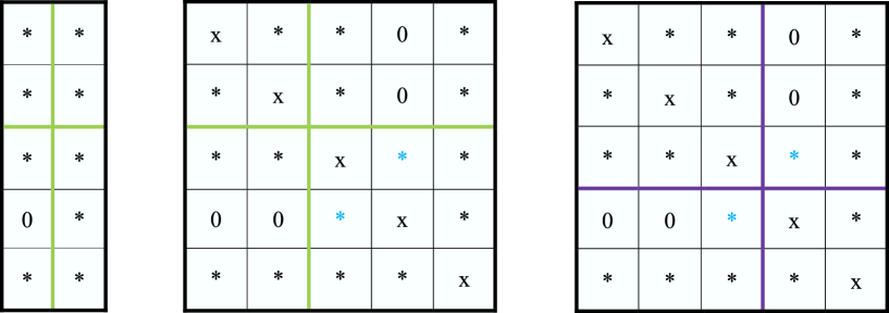
Figure 1: Zeros of the probability matrix with $n=5$ and $K_{*}=2$. Star symbols correspond to nonzero elements, the “x” symbols stand for the diagonal elements that are unavailable, the thick lines correspond to clustering assignments. Left panel: matrix $\Lambda$ with $(J_{*})_{1,1}=\{1,2\}$, $(J_{*})_{2,1}=\{3,5\}$, $(J_{*})_{1,2}=\{1,2\}$ and $(J_{*})_{2,2}=\{3,4,5\}$. Middle panel: matrix $P_{*}(Z_{*},K_{*})$ with true clustering, $(\breve{J}_{*})_{2,1}^{c}(Z_{*})=\{4\}$, $\hat{P}_{i,j}(Z_{*},K_{*})=0$ for $(i,j)\in\{(1,4),(2,4),(4,1),(4,2)\}$, so that, zero entries of the probability matrix are estimated by zeros. Right panel: matrix $P_{*}(\hat{Z},K_{*})$ with node 3 erroneously placed into community 1. The values of $(P_{*})_{4,3}$ and $(P_{*})_{3,4}$ are nonzero. If $A_{3,4}=A_{4,3}=0$, then $\{4\}\in\breve{J}_{2,1}^{c}(\hat{Z})$ and $\hat{P}_{i,j}(\hat{Z},K_{*})=0$ for $(i,j)\in\{(1,4),(2,4),(3,4),(4,1),(4,2),(4,3)\}$, hence, zero entries of $P_{*}$ are still estimated by the identical zeros. However, if $A_{4,3}=A_{3,4}=1$, then zero elements $(P_{*})_{4,1}$, $(P_{*})_{4,2}$, $(P_{*})_{1,4}$ and $(P_{*})_{2,4}$ are estimated by positive values.

Unfortunately, $K_{*}$ and $Z_{*}$ are unknown and, hence, $\hat{J}_{K}(Z,K)=\breve{J}_{K}(Z,K)$ may not always be the best estimator. In order to understand this, consider, for example, the situation displayed in Figure 1 where $n=5$, $K_{*}=2$ and, under the true clustering, one has $n_{1}=2$ and $n_{2}=3$. Vectors $\Lambda_{2,1}$ has one zero element, so that $(J_{*})_{1,1}=\{1,2\}$, $(J_{*})_{2,1}=\{3,5\}$, $(J_{*})_{1,2}=\{1,2\}$ and $(J_{*})_{2,2}=\{3,4,5\}$ (left panel) leading to $(J_{*})^{(1,1)}=\{(1,1),(1,2),(2,1),(2,2),\}$, $(J_{*})^{(2,1)}=\{(3,1),(3,2),(5,1),(5,2)\}$, $(J_{*})^{(1,2)}=\{(1,3),(2,3),(1,5),(2,5)\}$ and $(J_{*})^{(2,2)}=\{(3,3),(3,4),(3,5),(4,3),(4,4),(4,5),(5,3),\\ (5,4),(5.5)\}$ (middle panel). With the true clustering (middle panel), $(\breve{J}_{*})_{2,1}^{c}(Z_{*})=\{4\}$, so that $\hat{P}_{i,j}(Z_{*},K_{*})=0$ for $(i,j)\in\{(1,4),(2,4),(4,1),(4,2)\}$. Hence, zero entries of the probability matrix are estimated by zeros.

Consider now the situation where the third node has been erroneously placed into community 1 by clustering matrix $\hat{Z}$ (right panel). Then, we have $(J_{*})^{c}_{2,1}=\{4\}$ but $(\breve{J}_{*})_{2,1}^{c}(\hat{Z})$ is an empty set. If $A_{3,4}=A_{4,3}=0$, then $\{4\}\in\breve{J}_{2,1}^{c}(\hat{Z})$ and $\hat{P}_{i,j}(\hat{Z},K_{*})=0$ for $(i,j)\in\{(1,4),(2,4),(4,1),(4,2)\}$, hence, zero entries of $P_{*}$ are still estimated by the identical zeros. However, if $A_{4,3}=A_{3,4}=1$, then it is possible that zero elements $(P_{*})_{4,1}$, $(P_{*})_{4,2}$, $(P_{*})_{1,4}$ and $(P_{*})_{2,4}$ are estimated by positive values. For example, if $A_{5,1}=1$, $A_{5,2}=1$ and $A_{5,3}=1$, then $\hat{P}_{4,1}=0.3536$ and $\hat{P}_{4,2}=0.3536$ which leads to higher estimation errors than setting $\hat{P}_{4,1}=\hat{P}_{4,2}=0$. Therefore, it is reasonable to introduce a penalty that will lead to trimming the support of $\hat{P}(Z,K)$.

One can consider two kinds of penalties here: separable and non-separable. We say that a penalty $Pen(n,J,K)$ is separable if for any $K$ and any clustering matrix $Z$ that partitions $n$ nodes into $K$ communities of sizes $n_{k},k=1,\ldots,K$, one can write

$$\mbox{Pen}(n,J,K)=\mbox{Pen}^{(0)}(n,J,K)+\mbox{Pen}^{(1)}(n,K)\ \mbox{with}\ \mbox{Pen}^{(0)}(n,J,K)=\sum_{l=1}^{K}\,\sum_{k=1}^{K}\mathscr{F}(|J_{k,l}|,n_{k}),$$ (16)

where $J_{k,l}\equiv J_{k,l}(Z,K)$. Otherwise, the penalty is non-separable.

Lemma 2.

Let $(\hat{Z}_{K},\hat{J}_{K})$ be the solution of the optimization problem (13). If $Pen(n,J,K)$ is an increasing function of $|J|$ (for a non-separable penalty) or of $|J_{k,l}|,k,l=1,\ldots,K$ (for a separable penalty), then

$$\hat{J}_{k,l}(\hat{Z}_{K},K)\subseteq\breve{J}_{k,l}(\hat{Z}_{K},K)\subseteq(\breve{J}_{*})_{k,l}(\hat{Z}_{K},K),\quad\hat{J}(\hat{Z}_{K},K)\subseteq\breve{J}(\hat{Z}_{K},K)\subseteq\breve{J}_{*}(\hat{Z}_{K},K).$$ (17)

3 The Errors of Estimation and Clustering

3.1 The penalty

In what follows, we consider the separable and the non-separable penalties of the form (16) with the common $\mbox{Pen}^{(1)}(n,K)$ term, i.e.

$$\mbox{Pen}^{(a)}(n,J,K)=\mbox{Pen}^{(0,a)}(n,J,K)+\mbox{Pen}^{(1)}(n,K),$$ (18)

where a =s for the separable penalty and a = ns for the non-separable one, and

$$\mbox{Pen}^{(0,s)}(n,J,K) = \beta_{1}\displaystyle\sum_{k,l=1}^{K}|J_{k,l}|\ln(n_{k}e/|J_{k,l}|)+\beta_{2}K\displaystyle\sum_{k=1}^{K}\ln n_{k}$$ (19)

$$\mbox{Pen}^{(0,ns)}(n,J,K) = \beta_{1}|J|\ln(nKe/|J|)+2\beta_{2}\ln n$$ (20)

$$\mbox{Pen}^{(1)}(n,K) = \beta_{2}[n\ln K+\ln n].$$ (21)

Here, the separable penalty corresponds to $\mathscr{F}(|J_{k,l}|,n_{k})=\beta_{1}|J_{k,l}|\,\ln(n_{k}e/|J_{k,l}|)+\beta_{2}\ln n_{k}$ and the exact expressions for $\beta_{1}$ and $\beta_{2}$ are given in the proof of Theorem 1.

In the next two sections, we shall provide upper bounds for the errors of the solution of optimization problem (10) with the separable or the non-separable penalty (18), as well as upper bounds for the clustering error in the case of the separable penalty. While the separable penalty has some valuable properties (see Lemma 2), the non-separable penalty is much easier to interpret. Fortunately, as the statement below shows, under very nonrestrictive conditions, the penalties are within a constant factor of each other.

Lemma 3.

If $n\geq 8$ and $K\leq\sqrt{n/\ln n}$, then

$$\mbox{Pen}^{(ns)}(n,J,K)<(2+\beta_{1}/\beta_{2})\,\mbox{Pen}^{(s)}(n,J,K)<2\,(2+\beta_{1}/\beta_{2})\,\mbox{Pen}^{(ns)}(n,J,K).$$ (22)

3.2 The Estimation Errors

Theorem 1.

Let $(\hat{\Theta},\hat{Z},\hat{J},\hat{K})$ be a solution of optimization problem (10) with the penalty defined in (18). Construct the estimator $\hat{P}$ of $P_{*}$ of the form

$$\hat{P}=\mathscr{P}_{\hat{Z},\hat{K}}\ \hat{\Theta}(\hat{Z},\hat{J},\hat{K})\ \mathscr{P}_{\hat{Z},\hat{K}}^{T}$$ (23)

where $\mathscr{P}_{\hat{Z},\hat{K}}$ is the permutation matrix corresponding to $(\hat{Z},\hat{K})$. Then, for any $t>0$ and some absolute positive constants $\gamma$ and $\tilde{C}$, one has

$${\mathbb{P}}\left\{n^{-2}\,\|\hat{P}-P_{*}\|_{F}^{2}\leq n^{-2}\,H_{0}\,\mbox{Pen}(n,J_{*},K_{*})+n^{-2}\,\tilde{C}t\right\}\geq 1-3e^{-t},$$ (24)

$$n^{-2}\,{\mathbb{E}}\|\hat{P}-P_{*}\|_{F}^{2}\leq n^{-2}\,H_{0}\,\mbox{Pen}(n,J_{*},K_{*})+3n^{-2}\,\tilde{C}.$$ (25)

The exact expressions for $H_{0}$ and $\tilde{C}$ are given in the proof of Theorem 1.

Observe that, due to Lemma 3, the separable and non-separable penalties are within a constant factor of each other, so that Theorem 1 implies that the estimation error is proportional to $\mbox{Pen}(n,J_{*},K_{*})$ where

$$\mbox{Pen}(n,J,K)\asymp\mbox{Pen}^{(ns)}(n,J,K)\asymp n\ln K+|J|\,\ln(nKe/|J|)+\ln n.$$ (26)

The first term in (26) is due to the clustering errors, the second term quantifies the difficulty of finding $|J|$ nonzero elements among $nK$ elements of matrix $\Lambda\in[0,1]^{n\times K}$ and estimating them, while the term $\ln n\asymp\ln(nK)$ stands for the difficulty of finding the cardinality of the set $|J|$, and it is always dominated by the first two terms in (26).

Since each node is connected to at least one community with a nonzero probability, one has $n\leq|J|\leq nK$. In the (non-sparse) PABM, $|J|=nK$ and the second term in (26) is always asymptotically larger than the other two terms, as $n\to\infty$. In SPABM, the second term in (26) dominates the first term only if $K=1$ or $|J|/n\to\infty$ as $n\to\infty$. However, if $K>1$ and $|J|\asymp n$, then both terms are of the equal asymptotic order. If $K\to\infty$ and $|J|\asymp n$ as $n\to\infty$, then SPABM has the error $O(n\ln K)$ which is asymptotically smaller than $O(nK)$ error of PABM.

3.3 Detectability of clusters

In order one can detect clusters, the vectors $\Lambda^{(k,l)}$, $l=1,\ldots,K$, should be sufficiently different for every $k=1,\ldots,K$. Assume that $K=K_{*}$ is known and that the following condition holds.

Assumption A1.   For any $k=1,\ldots,K$, vectors ${\Lambda}^{(k,1)},\ldots,{\Lambda}^{(k,K)}$ are linearly independent.

Under Assumption A1, the true clusters are detectable.

Lemma 4.

Let $Z_{*}\in{\mathcal{M}}_{n,K}$ be the true clustering matrix, and $Z\in{\mathcal{M}}_{n,K}$ be an arbitrary clustering matrix. Let $J_{*}=J_{*}(Z_{*})$ be the true set of indices of nonzero elements, and $\breve{J}_{*}=\breve{J}_{*}(Z)$ be the set of indices of nonzero elements, defined in (LABEL:eq:brJ), which is associated with a clustering matrix $Z\in{\mathcal{M}}_{n,K}$. If Assumption A1 holds and the network is connected, then

$$\small{\sum_{k,l=1}^{K}\,\left\|P_{*}^{(k,l)}(Z_{*})-\Pi_{(1)}\left(\Pi_{J_{*}^{(k,l)}}(P_{*}^{(k,l)}(Z_{*})\right)\right\|_{F}^{2}\leq\sum_{k,l=1}^{K}\,\left\|P_{*}^{(k,l)}(Z)-\Pi_{(1)}\left(\Pi_{\breve{J}_{*}^{(k,l)}}(P_{*}^{(k,l)}(Z)\right)\right\|_{F}^{2}}$$ (27)

where, for any matrix $B$, $\Pi_{(1)}(B)$ is its rank one approximation and $\Pi_{J}$ is its projection on the set of indices defined by $J$. Moreover, equality in (27) occurs if and only if matrices $Z$ and $Z_{*}$ coincide up to a permutation of columns.

3.4 The Clustering Errors

In order to evaluate the clustering error when clustering is applied to the adjacency matrix, we assume that the true number of classes $K=K_{*}$ is known. Then $\hat{Z}\equiv\hat{Z}_{K}$ is a solution of the optimization problem (13).

Let $Z_{*}\in{\mathcal{M}}_{n,K}$ be the true clustering matrix and $Z_{*}\in{\mathcal{M}}_{n,K}$ be any other clustering matrix. Then the proportion of misclustered nodes can be evaluated as

$$\mbox{Err}(Z,Z_{*})=(2n)^{-1}\,\underset{\mathscr{P}_{K}\in\mathcal{P}_{K}}{\min}\|Z\mathscr{P}_{K}-Z_{*}\|_{1}=(2n)^{-1}\,\underset{\mathscr{P}_{K}\in\mathcal{P}_{K}}{\min}\|Z\mathscr{P}_{K}-Z_{*}\|_{F}^{2}$$ (28)

where $\mathcal{P}_{K}$ is the set of permutation matrices $\mathscr{P}_{K}:\{1,2,\cdots,K\}\longrightarrow\{1,2,\cdots,K\}$. Let

$$\Upsilon(Z_{*},\delta_{n})=\left\{Z\in\mathcal{M}_{n,K}:(2n)^{-1}\,\underset{\mathscr{P}_{K}\in\mathcal{P}_{K}}{\min}\|Z\mathscr{P}_{K}-Z_{*}\|_{1}\geq\delta_{n}\right\}$$ (29)

be the set of clustering matrices with the proportion of misclassified nodes being at least $\delta_{n}\in(0,1)$.

The success of clustering in (13) relies upon the fact that matrix $P_{*}$ is a collection of $K^{2}$ rank one blocks, so that the operator and the Frobenius norms of each block are the same. On the other hand, if clustering were incorrect, the ranks of the blocks would increase which would lead to the discrepancy between their operator and Frobenius norms. In particular, the following statement is true.

Theorem 2.

Let $K=K_{*}\geq 2$ be the true number of clusters. $Z_{*}\in{\mathcal{M}}_{n,K}$ be the true clustering matrix and Assumption A1 hold. Let $J_{*}=J_{*}(Z_{*})$ be the true set of indices of nonzero elements, and $\breve{J}_{*}=\breve{J}_{*}(Z)$ be the set of indices of nonzero elements, defined in (LABEL:eq:brJ), which is associated with a clustering matrix $Z\in{\mathcal{M}}_{n,K}$. Let $\hat{Z}\equiv\hat{Z}_{K}$ be a solution of the optimization problem (13) and $\delta_{n}\to 0$ as $n\to\infty$. If there exists $\alpha_{n}\in(0,1/2)$ and absolute positive constants $H_{1}$ and $H_{2}$, independent of $K$, $n$, $J_{*}$, $\breve{J}_{*}(Z)$, $\delta_{n}$ and $\alpha_{n}$, such that

$$\|P_{*}\|_{F}^{2} \geq\underset{Z\in\Upsilon(Z_{*},\delta_{n})}{\max}\left[(1+\alpha_{n})\,\sum_{k,l=1}^{K}\|P_{*}^{(k,l)}(Z)\|_{op}^{2}+\frac{H_{1}}{\alpha_{n}}\,|\breve{J}_{*}(Z)|\ln\left(\frac{nKe}{|\breve{J}_{*}(Z)|}\right)\right]$$

$$+\frac{H_{1}}{\alpha_{n}}\,\left(|J_{*}|+n\ln K\right)+H_{2}|J_{*}|\ln\left(\frac{nKe}{|J_{*}|}\right)$$ (30)

then, with probability at least $1-2K^{-n}$, the proportion of the nodes, misclassified by $\hat{Z}$, is at most $\delta_{n}$.

Example 1.

In order to see what condition (30) means, we consider a simple example. We study the sparse PABM with $K=2$, and $Z_{*}\in{\mathcal{M}}_{n,2}$ with equal size communities $N=n/2$. Assume that $\Lambda^{(k,k)}=\sqrt{a}\,1_{N}$, $k=1,2$, while elements $\Lambda^{(k,l)}_{i}$ of vectors $\Lambda^{(k,l)}$, $k\neq l$, are equal to $\sqrt{b}$ if $i\in J_{k}$, $k=1,2$, and equal to zero otherwise. Examine the case of an assortative network, where $a\equiv a_{n}$, $b\equiv b_{n}$ and $b/a=\rho\equiv\rho_{n}\leq 1$. Denote $J=J_{1}\cup J_{2}$ and note that the cardinality of the set of nonzero elements of matrix $\Lambda$ is equal to $2N+|J|$ with $|J|=|J_{1}|+|J_{2}|$. Denote the overall proportion of nonzero entries in vectors $\Lambda^{(1,2)}$ and $\Lambda^{(2,1)}$ by $\gamma$, and the proportion of zero entries in vectors $\Lambda^{(1,2)}$ and $\Lambda^{(2,1)}$ by $s$:

$$\gamma=|J|/n=(|J_{1}|+|J_{2}|)/(2N),\quad s=1-\gamma.$$

Below we examine what condition (30) of Theorem 2 means for different values of $s$ and $\rho$. Assume that the connection probabilities are not too small, specifically, that

$$\lim_{n\to\infty}na_{n}^{2}=\infty.$$ (31)

Let $\delta_{n}\equiv\delta=\delta_{1}+\delta_{2}$. Let $Z\in\Upsilon(Z_{*},\delta_{n})\subset{\mathcal{M}}_{n,2}$ be an arbitrary incorrect clustering matrix and, according to $Z$, $\check{N}_{k}=N\delta_{k}$ nodes are moved erroneously from class $k$ to class $l$, $l\neq k$, and $\tilde{N}_{k}=N(1-\delta_{k})$ nodes remain correctly in class $k$. Then, according to $Z$, community $k$ has $\tilde{N}_{k}+\check{N}_{l}$ nodes, $k=1,2$, $k\neq l$, and the proportion of misclassified nodes is equal to $(\delta_{1}N+\delta_{2}N)/n=\delta/2$. Denote the subsets of nodes corresponding to nonzero elements of vector $\Lambda^{(k,l)}$, that correctly stay in class $k$ and those that are misclassified into community $l$, $l\neq k$, by $\tilde{J}_{k}$ and $\check{J}_{k}$, respectively. Then $J_{k}=\tilde{J}_{k}\cup\check{J}_{k}$, $k=1,2$. Denote

$$\tilde{\beta}_{k}=|\tilde{J}_{k}|/|\tilde{N}_{k}|,\ \ \check{\beta}_{k}=|\check{J}_{k}|/|\check{N}_{k}|,\quad k=1,2,$$ (32)

and note that $\tilde{\beta}_{k},\check{\beta}_{k}\in[0,1]$. Then, for any $Z\in{\mathcal{M}}_{n,2}$ with equal class sizes and the proportion of misclassified nodes being $\delta/2$, one has

$$\|P_{*}\|_{F}^{2}-(1+\alpha_{n})\,\sum_{k,l=1}^{2}\|P_{*}^{(k,l)}(Z)\|_{op}^{2}\geq\check{C}\,a^{2}n^{2}(\Delta_{n}(Z)-16\,\alpha_{n}),$$ (33)

where $\check{C}$ is an absolute constant, $\alpha\equiv\alpha_{n}$ and

$$\Delta_{n}(Z)=\delta_{1}^{2}\,(1-\rho_{n}^{2}\,\check{\beta}_{1}^{2}\,\tilde{\beta}_{2}^{2})^{2}+\delta_{2}^{2}\,(1-\rho_{n}^{2}\,\tilde{\beta}_{1}^{2}\,\check{\beta}_{2}^{2})^{2}.$$ (34)

The proof of the inequality (33) is given in the Appendix.

Note that, in this example, the right hand side of (30) reduces to $H_{1}\,n\,\alpha_{n}^{-1}+H_{2}n$, so we need to show that

$$a^{2}n^{2}\Delta_{n}(Z)\geq 16\,a^{2}n^{2}\,\alpha_{n}+\tilde{H}_{1}\,n\,\alpha_{n}^{-1}+\tilde{H}_{2}n,$$ (35)

for some $\alpha_{n}\in(0,1/2)$ and absolute positive constants $\tilde{H}_{1}$ and $\tilde{H}_{2}$. It is easy to see that the right hand side of (35) is minimized by $\alpha_{n}=C_{\alpha}\,/(a_{n}\sqrt{n})\in(0,1/2)$, and (35) appears as

$$a_{n}\sqrt{n}\ \Delta_{n}(Z)\geq\tilde{H}_{3}$$ (36)

for some absolute positive constant $\tilde{H}_{3}$. Below, we examine when this condition can be satisfied for $\delta_{n}\to 0$ as $n\to\infty$.

First, we consider the case when $s=0$, so that $\gamma=1$ and there is no structural sparsity. In this case, $\check{\beta}_{k}=\tilde{\beta}_{k}=1$, $k=1,2$, and, due to $\delta_{1}^{2}+\delta_{2}^{2}\geq(\delta_{1}+\delta_{2})^{2}/2=\delta^{2}/8$, one obtains from (34) that $\Delta_{n}(Z)\asymp\delta_{n}^{2}(1-\rho_{n}^{2})^{2}$. Hence, (36) becomes $a_{n}\sqrt{n}\,\delta_{n}^{2}(1-\rho_{n}^{2})^{2}\geq\tilde{H}_{3}$, so that

$$\delta_{n}^{2}\asymp\left[na_{n}^{2}(1-\rho_{n}^{2})^{2}\right]^{-1}\to 0\quad\mbox{if}\quad na_{n}^{2}(1-\rho_{n}^{2})^{2}\to\infty\quad(n\to\infty).$$ (37)

The latter implies that either $a_{n}$ should be asymptotically larger than $n^{-1/2}$ or the ratio $\rho_{n}=b_{n}/a_{n}$ should be separated from one.

Now, consider $s>0$, so that $\gamma<1$. In this case we need the minimal possible value of $\Delta_{n}(Z)$ over $Z\in\Upsilon(Z_{*},\delta_{n})$ to satisfy condition (36). To formalize this notion, we introduce

$$\widehat{F}(\gamma,\delta,\rho,a,n) =\min\left\{\delta_{1}^{2}\,(1-\rho_{n}^{2}\,\check{\beta}_{1}^{2}\,\tilde{\beta}_{2}^{2})^{2}+\delta_{2}^{2}\,(1-\rho_{n}^{2}\,\tilde{\beta}_{1}^{2}\,\check{\beta}_{2}^{2})^{2}\right\}$$

s.t. $$0\leq\tilde{\beta}_{k}\leq 1,\ 0\leq\check{\beta}_{k}\leq 1,\ \tilde{\beta}_{k},\check{\beta}_{k}\ \mbox{given by}\ \eqref{eq:tcbek},\ \ k=1,2,$$

$$\delta_{k}\geq 0,\ k=1,2,\ \delta_{1}+\delta_{2}=\delta\leq 1/2$$

$$\tilde{\beta}_{1}(1-\delta_{1})+\tilde{\beta}_{2}(1-\delta_{2})+\check{\beta}_{1}\delta_{1}+\check{\beta}_{2}\delta_{2}=2\gamma$$ (38)

In order the proportion of clustering errors is bounded above by $\delta_{n}\to 0$, one needs

$$\widehat{F}(\gamma,\delta_{n},\rho_{n},a_{n},n)\asymp\left(a_{n}^{2}n\right)^{-1/2},\quad(n\to\infty).$$ (39)

Consider the case when $s<1/2$, so that $1/2<\gamma<1$. If $\delta_{n}\to 0$, then, for $n$ large enough, one has $\delta_{n}\leq 2(\gamma-1/2)$ and, hence, $2\gamma\geq 1+\delta_{n}$. Set $\delta_{1}=\delta$, $\delta_{2}=0$, $\check{\beta}_{1}=\tilde{\beta}_{2}=1$, $\tilde{\beta}_{1}=[2\gamma-(1+\delta)]/(1-\delta)$, $\check{\beta}_{2}=0$. It is easy to verify that conditions in (38) hold, so that $\widehat{F}(\gamma,\delta,\rho,a,n)\leq\delta^{2}(1-\rho_{n}^{2})^{2}$ and condition (39) is equivalent to (37), that occurs when there is no structural sparsity ($s=0$).

Now, let $s>1/2$, so that $0<\gamma<1/2$. Let $d=(1-2\gamma)/2$ and, if $\delta_{n}\to 0$, then, for $n$ large enough, one has $\delta_{n}\leq d$. Let $\gamma_{0}=(1-2d)/(1-d)<1.$ Then, $2\gamma/(1-\delta_{n})\leq\gamma_{0}$. By (38), obtain $\tilde{\beta}_{k}(1-\delta_{k})\leq 2\gamma$ and, hence, $\tilde{\beta}_{k}\leq 2\gamma/(1-\delta_{k})\leq\gamma_{0}$, $k=1,2$. Consequently, due to $\tilde{\beta}_{k},\check{\beta}_{k}\leq 1$, obtain

$$\widehat{F}(\gamma,\delta_{n},\rho_{n},a_{n},n)\geq(\delta_{1}^{2}+\delta_{2}^{2})(1-\rho_{n}^{2}\gamma_{0}^{2})^{2}\geq\delta_{n}^{2}(1-\gamma_{0}^{2})^{2}/2.$$

Since $\gamma_{0}$ is a non-asymptotic quantity, condition (39) holds for some $\delta_{n}\to 0$ as $n\to\infty$, whenever assumption (31) is satisfied. Therefore, if $s>1/2$, one has $\delta_{n}\to 0$ even if $\rho_{n}\to 1$ as $n\to\infty$.

The sparsity proportion of $s=1/2$ constitutes the so called “elbow” value, so the difficulty of clustering varies significantly for $s<1/2$ and $s>1/2$. Analysis of the conditions that ensure $\delta_{n}\to 0$ when $s=1/2$ requires more sophisticated tools, so we do not study $s=1/2$ in this paper.

Remark 1.

Non-constant connection probabilities. We remark that consideration of constant values for elements of vectors $\Lambda^{(k,k)}$ and $\Lambda^{(k,l)}$, $k,l=1,2$, $k\neq l$, is motivated by showing a clear pattern of the impact of sparsity on the clustering precision. Assumption that in-cluster and out-of-cluster connection probabilities take constant values are quite common in stochastic networks literature (see, e.g., Abbe (2018), Abbe et al. (2020a), Abbe et al. (2020b) and Ndaoud et al. (2020) among others). Indeed, if $\Lambda^{(k,k)}_{i}\geq\sqrt{a_{n}}$, and $\Lambda^{(k,l)}_{i}\leq\sqrt{b_{n}}$ if $i\in J_{k}$, $k=1,2$, $k\neq l$, and equal to zero otherwise, where $b_{n}/a_{n}=\rho_{n}\leq 1$, then conclusion of Example 1 that $\delta_{n}\to 0$ as $n\to\infty$ is still true, provided condition (31) holds and $s>1/2$. However, in the case of $s<1/2$, $\delta_{n}$ may tend to zero even if $s<1/2$, depending on the exact values of components of vectors $\Lambda^{(k,k)}$ and $\Lambda^{(k,l)}$. Studying the case of constant probabilities allowed us to show the benefits of structural sparsity more clearly.

4 Implementation of Clustering

In Section 2, we obtained an estimator $\hat{Z}$ of the true clustering matrix $Z_{*}$ as a solution of optimization problem (12). Minimization in (12) is somewhat similar to modularity maximization in Bickel and Chen (2009) or Zhao et al. (2012) in the sense that modularity maximization as well as minimization in (12) are NP-hard, and, hence, require some relaxation in order to obtain an implementable clustering solution.

In the case of the SBM and the DCBM, possible relaxations include semidefinite programming (see, e.g., Amini and Levina (2018) and references therein), variational methods (Celisse et al. (2012)) and spectral clustering and its versions (see, e.g., Joseph and Yu (2016), Lei and Rinaldo (2015) and Rohe et al. (2011) among others). Since in the case of SPABM, columns of matrix $P_{*}$ that correspond to nodes in the same class are neither identical, nor proportional, direct application of spectral clustering to matrix $P_{*}$ does not deliver the partition of the nodes. However, it is easy to see that the columns of matrix $P_{*}$ that correspond to nodes in the same community, form a matrix with $K$ rank-one blocks, hence, those columns lie in the subspace of the dimension at most $K$. Therefore, matrix $P_{*}$ is constructed of $K$ clusters of columns (rows) that lie in the union of $K$ distinct subspaces, each of the dimension $K$. For this reason, the subspace clustering presents a technique for obtaining a fast and reliable solution of optimization problem (12) (or (13)).

Subspace clustering has been widely used in computer vision and, for this reason, it is a very well studied and developed technique. Subspace clustering is designed for separation of points that lie in the union of subspaces. Let $\{X_{j}\in\mathbb{R}^{D}\}_{j=1}^{n}$ be a given set of points drawn from an unknown union of $K\geqslant 1$ linear or affine subspaces $\{S_{i}\}_{i=1}^{K}$ of unknown dimensions $d_{i}=\text{dim}(S_{i})$, $0<d_{i}<D$, $i=1,...,K$. In the case of linear subspaces, the subspaces can be described as $S_{i}=\{{\mbox{$x$}}\in\mathbb{R}^{D}:{\mbox{$x$}}={\mbox{$U$}}_{i}{\mbox{$y$}}\}$, $i=1,...,K,$ where ${\mbox{$U$}}_{i}\in\mathbb{R}^{D\times d_{i}}$ is a basis for subspace $S_{i}$ and ${\mbox{$y$}}\in\mathbb{R}^{d_{i}}$ is a low-dimensional representation for point $x$. The goal of subspace clustering is to find the number of subspaces $K$, their dimensions $\{d_{i}\}_{i=1}^{K}$, the subspace bases $\{{\mbox{$U$}}_{i}\}_{i=1}^{K}$, and the segmentation of the points according to the subspaces.

Several methods have been developed to implement subspace clustering such as algebraic methods (Boult and Gottesfeld Brown (1991), Ma et al. (2008), Vidal et al. (2005)), iterative methods (Agarwal and Mustafa (2004), Bradley and Mangasarian (2000), Tseng (2000)), and spectral clustering based methods (Elhamifar and Vidal (2009), Elhamifar and Vidal (2013), Favaro et al. (2011), Liu et al. (2013), Liu et al. (2010), Soltanolkotabi et al. (2014), Vidal (2011)). In this paper, we use the latter group of techniques.

Spectral clustering algorithms rely on construction of an affinity matrix whose entries are based on some distance measures between the points. In particular, in the case of the SBM, adjacency matrix itself serves as the affinity matrix, while for the DCBM, the affinity matrix is obtained by normalizing rows/columns of $A$. In the case of the subspace clustering problem, one cannot use the typical distance-based affinity because two points could be very close to each other, but lie in different subspaces, while they could be far from each other, but lie in the same subspace. One of the solutions is to construct the affinity matrix using self-representation of the points with the expectation that a point is more likely to be presented as a linear combination of points in its own subspace rather than from a different one. A number of approaches such as Low Rank Representation (see, e.g., Liu et al. (2013), Liu et al. (2010)) and Sparse Subspace Clustering (see, e.g., Elhamifar and Vidal (2013), Elhamifar and Vidal (2009)) have been proposed in the past decade for the solution of this problem.

In this paper, we use Sparse Subspace Clustering (SSC) since it allows one to take advantage of the knowledge that, for a given $K$, columns of matrix $P_{*}$ lie in the union of $K$ distinct subspaces, each of the dimension at most $K$. If matrix $P_{*}$ were known, the weight matrix $W$ would be based on writing every data point as a sparse linear combination of all other points by solving the following optimization problem

$$\mathop{\text{missing}}{min}_{W_{j}}\|W_{j}\|_{1}\hskip 14.22636pt\mbox{s.t.}\hskip 14.22636pt(P_{*})_{j}=\sum_{k\neq j}W_{kj}(P_{*})_{k}$$ (40)

In the case of data contaminated by noise, the SSC algorithm does not attempt to write data as an exact linear combination of other points. Instead, SSC can be built upon the solution of the elastic net problem

$$\widehat{W}_{j}\in\underset{W_{j}}{\text{argmin}}\left\{\left[\frac{1}{2}\|{A_{j}-AW_{j}}\|_{2}^{2}+\gamma_{1}\|W_{j}\|_{1}+\gamma_{2}\|W_{j}\|_{2}^{2}\right]\quad\mbox{s.t.}\quad W_{jj}=0\right\},\quad j=1,...,n,$$ (41)

where $\gamma_{1},\gamma_{2}>0$ are tuning parameters. The quadratic term stabilizes the LASSO problem by making the problem strongly convex, and therefore it has a unique minimum.

We solve (41) using the LARS algorithm Efron et al. (2004) implemented in SPAMS Matlab toolbox (see Mairal et al. (2014)). Given $\widehat{W}$, the affinity matrix is defined as $|\widehat{W}|+|\widehat{W}^{T}|$ where, for any matrix $B$, matrix $|B|$ has absolute values of elements of $B$ as its entries. The class assignment (clustering matrix) $Z$ is then obtained by applying spectral clustering to $|\widehat{W}|+|\widehat{W}^{T}|$. We elaborate on the implementation of the SSC in Section 5.1.

5 Simulations and Real Data Examples

5.1 Simulations on Synthetic Networks

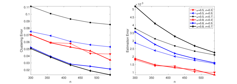
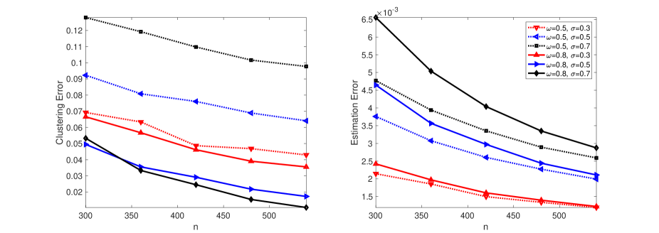
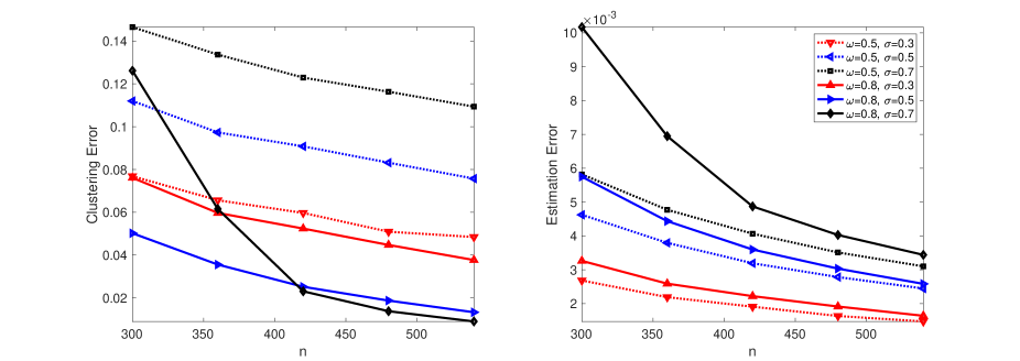
Figure 2: The clustering errors $\mbox{Err}(\hat{Z},Z)$ defined in (28) (left panels) and the estimation errors $n^{-2}\,\|{\hat{P}-P}\|_{F}^{2}$ (right panels) for $K=4$ (top), $K=5$ (middle) and $K=6$ (bottom) clusters. The errors are evaluated over 100 simulation runs. The number of nodes ranges from $n=300$ to $n=540$ with the increments of 60. Dashed lines represent the results for $\omega=0.5$ and solid lines represent the results for $\omega=0.8$; $\sigma=0.3$ (red), $\sigma=0.5$ (blue) and $\sigma=0.7$ (black).

In this section we evaluate the performance of our method using synthetic networks. We assume that the number of communities (clusters) $K$ is known and for simplicity consider a perfectly balanced model with $n/K$ nodes in each cluster. We generate each network from a random graph model with a symmetric probability matrix $P$ given by the SPABM model with a clustering matrix $Z$ and a block matrix $\Lambda$.

To generate synthetic networks, we start by producing a block matrix $\Lambda$ in (3) with random entries between 0 and 1. We use a parameter $\sigma$ as the proportion of nonzero entries in matrix $\Lambda$ to control the sparsity of networks. To do that, we set $\left\lfloor{nK\sigma}\right\rfloor$ smallest non-diagonal entries of $\Lambda$ zero. Then we multiply the non-diagonal blocks of $\Lambda$ by $\omega$, $0<\omega<1$, to ensure that most nodes in the same community have larger probability of interactions. As a result, matrix $P(Z,K)$ with blocks $P^{(k,l)}(Z,K)=\Lambda^{(k,l)}(\Lambda^{(l,k)})^{T}$, $k,l=1,\ldots,K$, has larger entries mostly in the diagonal blocks than in the non-diagonal blocks and some zero rows (columns) in the non-diagonal blocks. The parameter $\omega$ is the heterogeneity parameter. Indeed, if $\omega=0$, the matrix $P_{*}$ is strictly block-diagonal, while in the case of $\omega=1$, there is no difference between entries in diagonal and nonzero entries in non-diagonal blocks. Next, we generate a random clustering matrix $Z\in{\mathcal{M}}_{n,K}$ corresponding to the case of equal community sizes and the permutation matrix $\mathscr{P}_{Z,K}$ corresponding to the clustering matrix $Z$. Subsequently, we scramble rows and columns of $P(Z,K)$ to create the probability matrix $P=\mathscr{P}_{Z,K}P(Z,K)\mathscr{P}_{Z,K}^{T}$. Finally we generate the lower half of the adjacency matrix $A$ as independent Bernoulli variables $A_{ij}\sim\text{Ber}(P_{ij})$, $i=1,\ldots,n,j=1,\ldots,i-1$, and set $A_{ij}=A_{ji}$ when $j>i$. In practice, the diagonal elements of matrix $A$ are unavailable, so we estimate $\mbox{diag}(P)$ without their knowledge.

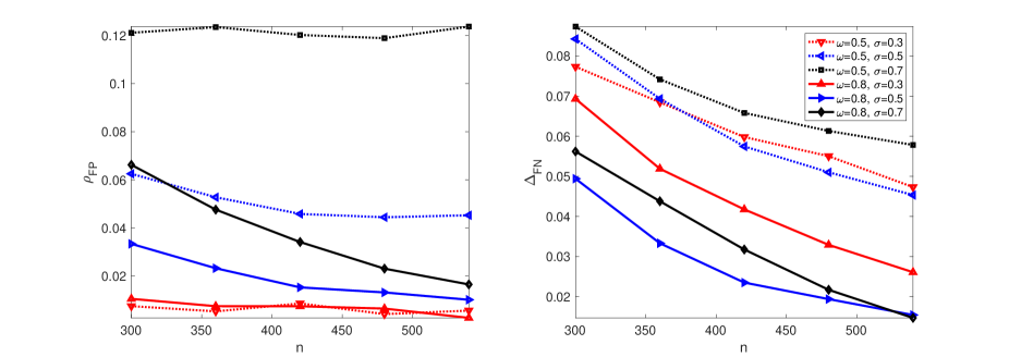
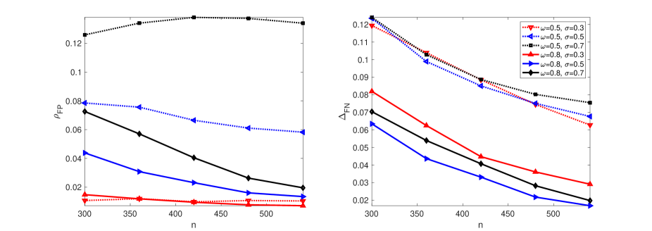
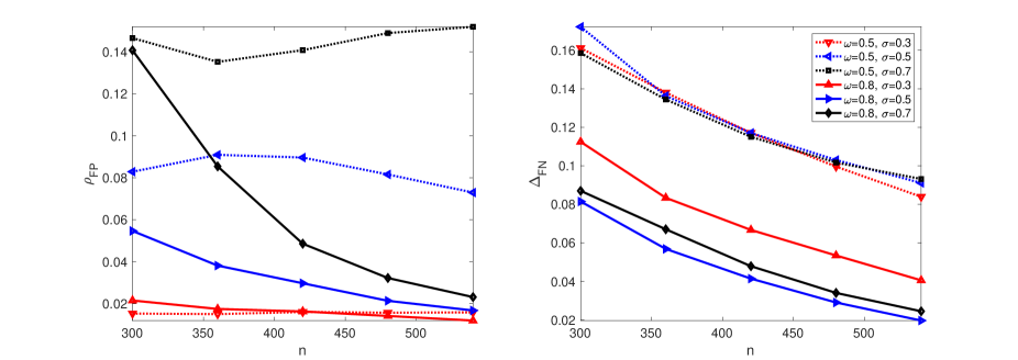
Figure 3: The false positive rates $\rho_{FP}$ (left panels) and the rates $\Delta_{FN}$ (right panels) for $K=4$ (top), $K=5$ (middle) and $K=6$ (bottom) clusters. The rates are evaluated over 100 simulation runs. The number of nodes ranges from $n=300$ to $n=540$ with the increments of 60. Dashed lines represent the results for $\omega=0.5$ and solid lines represent the results for $\omega=0.8$; $\sigma=0.3$ (red), $\sigma=0.5$ (blue) and $\sigma=0.7$ (black).

Now we use SSC to find the clustering matrix $\hat{Z}$. Since the diagonal elements of matrix $A$ are unavailable, we initially set $A_{ii}=0$, $i=1,...,n$, and solve optimization problem (41) with $\gamma_{1}=30\rho(A)$ and $\gamma_{2}=125(1-\rho(A))$, where $\rho(A)$ is the density of matrix $A$, the proportion of nonzero entries of $A$. The values of $\gamma_{1}$ and $\gamma_{2}$ have been obtained empirically by testing on synthetic networks. After matrix $\widehat{W}$ of weights is evaluated, we obtain the clustering matrix $\hat{Z}$ by applying spectral clustering to $|\widehat{W}|+|\widehat{W}^{T}|$, as it was described in Section 4. In this paper, we use the normalized cut algorithm Shi and Malik (2000) to perform spectral clustering. Given $\hat{Z}$, we generate matrix $A(\hat{Z},K)=\mathscr{P}_{\hat{Z},K}^{T}A\mathscr{P}_{\hat{Z},K}$ with blocks $A^{(k,l)}(\hat{Z},K)$, $k,l=1,\ldots,K$, and obtain $\hat{\Theta}^{(k,l)}(\hat{Z},K)$ by using the rank one approximation for each of the blocks. Finally, we estimate matrix $P$ by $\hat{P}=\hat{P}(\hat{Z},\hat{K})$ using formula (23) with $\hat{K}=K$.

Figure 2 represents the accuracy of SSC in terms of the average estimation errors $n^{-2}\,\|{\hat{P}-P}\|_{F}^{2}$ and the average clustering errors $\mbox{Err}(\hat{Z},Z)$ defined in (28) for $K=4,5$ and 6, respectively, and the number of nodes ranging from $n=300$ to $n=540$ with the increments of 60. The left panels display the clustering errors $\mbox{Err}(\hat{Z},Z)$ while the right ones exhibit the estimation errors $n^{-2}\,\|{\hat{P}-P}\|_{F}^{2}$, as functions of the number of nodes, for two different values of the parameter $\omega$: $\omega=0.5$ (dashed lines) and 0.8 (solid lines) and three different values of the parameter $\sigma$: $\sigma=0.3$ (red lines), 0.5 (blue lines), and 0.7 (black lines).

Figure 2 shows that sparsity has a different affect on estimation and clustering errors. It is easy to see that as sparsity increases ($\sigma$ decreases), the estimation errors decrease. On the other hand, the difficulty of clustering depends on combination of the sparsity parameter $\sigma$ and the heterogeneity parameter $\omega$. Specifically, a denser network is easier to cluster when the network is more diverse (the heterogeneity parameter $\omega$ is larger), while for a very sparse network, heterogeneity of the network does not play much of a role. Indeed, in all three graphs in the left half of Figure 2, the red curves, corresponding to the most sparse case ($\sigma=0.3$), are close together while the black curves, corresponding to the least sparse case ($\sigma=0.7$), are further apart. The graphs also show the effect of the number of clusters $K$ on the clustering errors. Indeed, for large $K$ ($K=6$), when $n$ is small ($n<420$), sparser network is not harder to cluster than denser one, perhaps because the diverse sparsity patterns make the network less uniform. In summary, the difficulty of clustering depends on the interplay between sparsity and heterogeneity of the network.

Our procedure does not estimate the set $J$ explicitly. Instead, we set $\hat{J}=\breve{J}=\bigcup_{k,l=1}^{K}\breve{J}_{k,l}$ where $\breve{J}_{k,l}$ is defined in (LABEL:eq:brJ). Our next objective is to evaluate how accurate $\breve{J}$ is, as an estimator of $J_{*}$. While there are several ways for doing this, below we use two measures, the false positive rate $\rho_{FP}$, defined as the proportion of zero entries in $P_{*}$ that are estimated by non-zeros in $\hat{P}$, and $\Delta_{FN}=\|P_{*}\|_{F}^{-1}\|X_{*}\|_{F}$, where $\|X_{*}\|_{F}$ is the Frobenius norm of nonzero entries in $P_{*}$ that are estimated by zeros in $\hat{P}$. The reports on the accuracies of estimating $J_{*}$ are presented in Figure 3. The left panels display $\rho_{FP}$ while the right ones exhibit $\Delta_{FN}$, as functions of the number of nodes for the same settings as in Figure 2.

The left panels of Figure 3 demonstrate that the proportion of false positives $\rho_{FP}$ decreases as the network becomes more and more sparse and more heterogeneous (the proportions of false positives are smaller for smaller values of $\sigma$ and larger values of $\omega$). Again, the same as for Figure 2, the pattern emerges only when the number of nodes per community reaches some critical threshold. Indeed, as the bottom left panel of Figure 3 shows, the false positive rate is high, when the number of nodes is small. The right hand side panels of Figure 3 show that $\Delta_{FN}$, the relative norm of nonzero entries of $P_{*}$ estimated by zeros, is minimal for the moderately sparse network $\sigma=0.5$ and becomes smaller when the network is more heterogeneous. One can also notice that the values of $\Delta_{FN}$ are almost independent of $\sigma$ when the network is relatively homogeneous ($\omega=0.5$) but become more diverse when the network becomes more diverse ($\omega=0.8$).

Remark 2.

Unknown number of clusters. In our previous simulations we treated the true number of clusters as a known quantity. However, we can actually use $\hat{P}$ to obtain an estimator $\hat{K}$ of $K$ by solving, for every suitable $K$, the optimization problem (14), which can be equivalently rewritten as

$$\hat{K}=\mathop{\text{missing}}{argmin}_{K}\{\|{\hat{P}-A}\|_{F}^{2}+\mbox{Pen}(n,J,K)\}.$$ (42)

The penalties $\mbox{Pen}(n,J,K)$ defined in (18) are, however, motivated by the objective of setting it above the noise level with a very high probability. In our simulations, we also study the selection of an unknown $K$ using an empirical version of this penalty

$$\mbox{Pen}(n,J,K)=\rho(A)nK\sqrt{\ln n\,(\ln K)^{3}}.$$ (43)

In order to assess the accuracy of $\hat{K}$ as an estimator of $K$, we evaluated $\hat{K}$ as a solution of optimization problem (42) with the penalty (43) in each of the previous simulations settings over 100 simulation runs. Table 1 in Section A.1 of the Appendix presents the relative frequencies of the estimators $\hat{K}$ of $K_{*}$ for $K_{*}$ ranging from 3 to 5, $n=360$ and 480 and $\omega=0.5$ and 0.8 and $\sigma=0.4$, 0.6 and 0.8. Table 1 confirms that for majority of settings, $\hat{K}=K_{*}$, i.e., the estimated and the true number of clusters coincide with high probability.

We would like to point out that the problem (41) of finding weights is indeed strongly convex and it leads to a unique set of weights for every column of the adjacency matrix. However, the subsequent spectral clustering is not convex since it requires application of the $K$-means clustering to the main $K$ eigenvectors of the weight matrix. The subspace clustering is carried out with a fixed number of clusters. The number of clusters is then found as a solution of the discrete optimization problem (14). Therefore, even with the same adjacency matrix, due to random initialization of the $K$-means algorithm, the values of $\hat{K}$ may vary.

5.2 Real Data Examples

     

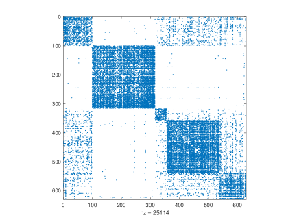
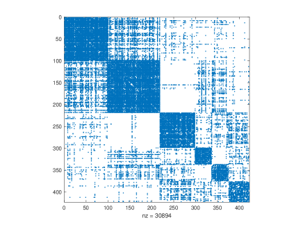
Figure 4: The adjacency matrices of the ego-network with 25114 nonzero entries and 5 clusters (left) and the brain network with 30894 nonzero entries and 6 clusters (right) after clustering

In this section, we report the performance of SSC and our estimation procedure when they are applied to two real life networks, an ego-network and a human brain network.

To study the ego-network, we use the dataset described comprehensively in Leskovec and Mcauley (2012). An ego-network is a social network of a single person, with the exclusion of the person generating this network. Users of social networking sites are usually provided with a tool that allows them to organize their networks into categories, referred to, in Leskovec and Mcauley (2012), as social circles. Practically all major social networking cites provide such functionality, for example, “circles” on Google+, and “lists” on Facebook and Twitter. Examples of such circles include university classmates, sports team members, relatives, etc. Once circles are created by a user, they can be utilized, for example, for content filtering (e.g. to filter status updates posted by distant acquaintances) or for privacy (e.g., to hide personal information from coworkers).

In this paper, we attempt to recover social circles of an ego-network when only binary connection data is available. In particular, we formulate the problem of circle detection as a clustering problem on an individual ego-network. In principle, circles can overlap or a circle can be a subset of another circle, hence, as an example in this paper, we study an ego-network with only few nodes overlap between the circles which does not affect the performance of the clustering method. Specifically, we study an ego-network from Facebook where user profiles are treated as nodes and a friendship between two user profiles is considered as an edge between them. Since a friendship is a mutual tie, the ego-network is undirected. The ego-network studied in this paper, has 777 nodes with 17 circles, each circle containing between 2 to 225 nodes. For our study, we extract the five largest circles of the this network, obtaining a network with 629 nodes and 12557 edges. We carried out clustering of the nodes using the SSC and compared the clustering assignments of SSC with the true class assignments. The SSC provides 85% accuracy. In addition, we applied formula (42) with $K$ ranging from 2 to 6 to the adjacency matrix with the randomly permuted rows (columns), obtaining the true number of clusters with 100% accuracy over 100 runs. Figure 4 shows the adjacency matrix of the graph after clustering (left), which confirms that the network indeed follows the SPABM. Indeed, the SPABM is a very appropriate model for this example since users display different degrees of connections to users in other circles, and, furthermore, the network is sparse, which justifies the application of the SPABM.

Our second example involves analyzing a human brain functional network, constructed on the basis of the resting-state functional MRI (rsfMRI). We use the the brain connectivity dataset presented as a GroupAverage rsfMRI matrix described in Crossley et al. (2013). In this dataset, the brain is partitioned into 638 distinct regions and a weighted graph is used to characterize the network topology. Nicolini et al. (2017) developed a new Asymptotical Surprise method, which is applied for clustering of the weighted graph. Asymptotical Surprise detects 47 communities ranging from 1 to 133. Since the true clustering as well as the true number of clusters are unknown for this dataset, we treat the results of the Asymptotical Surprise as the ground truth.

In order to generate a binary network, we set all nonzero weights to one in the GroupAverage rsfMRI matrix, obtaining a network with 18625 undirected edges. For evaluating the performance of SSC on this network, we extract 6 largest communities derived by the Asymptotical Surprise, obtaining a network with 422 nodes and 15447 edges. Applying (42), with K ranging from 2 to 10, to the adjacency matrix with the randomly permuted rows (columns), we recovered the true number of clusters with 64% accuracy over 100 simulation runs. For this true number of communities, our version of the SSC detects the true communities with 94% accuracy. Figure 4 (right) displays the adjacency matrix of the network after clustering, showing that the network is very sparse, thus, justifying application of the SPABM to the data.

Acknowledgments

The authors of the paper were partially supported by National Science Foundation (NSF) grants DMS-1712977 and DMS-2014928. We would also like to thank Drs. Nicolini, Bordier and Bifone for providing the brain dataset together with the results of their clustering algorithm.

A

A.1 Accuracy of Estimating the Number of Communities

Table 1 below presents the relative frequencies of the estimators $\hat{K}$ of $K_{*}$ for $K_{*}$ ranging from 3 to 5, $n=360$ and 480, $\omega=0.5$ and 0.8, and $\sigma=0.4$, 0.6 and 0.8. Table 1 confirms that for majority of settings, the estimated and the true number of clusters are equal, $\hat{K}=K_{*}$, with high probability.

		$n=360$
		$\omega=0.5$			$\omega=0.8$
$K_{*}$	$\hat{K}$	$\sigma=0.4$	$\sigma=0.6$	$\sigma=0.8$	$\sigma=0.4$	$\sigma=0.6$	$\sigma=0.8$
	2	0.01	0	0.01	0	0	0
	3	0.49	0.62	0.62	0.54	0.79	0.76
3	4	0.31	0.27	0.30	0.39	0.17	0.18
	5	0.15	0.09	0.06	0.06	0.04	0.06
	6	0.04	0.02	0.01	0.01	0	0
	2	0	0	0	0	0	0
	3	0.01	0.01	0.05	0	0	0.01
4	4	0.66	0.74	0.66	0.72	0.85	0.81
	5	0.22	0.22	0.25	0.23	0.15	0.16
	6	0.11	0.03	0.04	0.05	0	0.02
	2	0	0	0.02	0	0	0
	3	0	0	0.03	0	0	0
5	4	0.05	0.07	0.23	0	0	0.08
	5	0.70	0.69	0.54	0.74	0.84	0.84
	6	0.25	0.24	0.18	0.26	0.16	0.08
		$n=480$
		$\omega=0.5$			$\omega=0.8$
$K_{*}$	$\hat{K}$	$\sigma=0.4$	$\sigma=0.6$	$\sigma=0.8$	$\sigma=0.4$	$\sigma=0.6$	$\sigma=0.8$
	2	0	0	0	0	0	0
	3	0.64	0.62	0.60	0.54	0.73	0.76
3	4	0.26	0.17	0.31	0.32	0.24	0.19
	5	0.08	0.19	0.07	0.10	0.01	0.05
	6	0.02	0.02	0.02	0.04	0.02	0
	2	0	0	0	0	0	0
	3	0.01	0	0	0	0	0
4	4	0.64	0.68	0.76	0.69	0.74	0.83
	5	0.21	0.30	0.21	0.23	0.24	0.17
	6	0.14	0.02	0.03	0.08	0.02	0
	2	0	0	0	0	0	0
	3	0	0	0.02	0	0	0
5	4	0.04	0.01	0.21	0	0	0.05
	5	0.65	0.78	0.65	0.77	0.89	0.86
	6	0.31	0.21	0.12	0.23	0.11	0.09

Table 1: The relative frequencies of the estimators $\hat{K}$ of $K_{*}$ for $K_{*}$ ranging from 3 to 5, $n=360$ and 480 and $\omega=0.5$ and 0.8 and $\sigma=0.4$, 0.6 and 0.8.

A.2 Proof of Theorem 1

Overview: The proof follows the standard oracle inequality strategy. We bound the error $\left\|\hat{P}-P_{*}\right\|_{F}^{2}$ by the random error term plus the difference between the values of the penalty function at $K_{*},J_{*}$ and $\hat{K}$, $\hat{J}$:

$$2\mbox{Tr}\left[(A-P_{*})^{T}(\hat{P}-P_{*})\right]+\mbox{Pen}(n,{J_{*}},K_{*})-\mbox{Pen}(n,{\hat{J}},\hat{K}).$$

Subsequently, we show that the random error term is bounded above by the sum of the $\mbox{Pen}(n,{\hat{J}},\hat{K})$ and a small multiple of $\left\|\hat{P}-P_{*}\right\|_{F}^{2}$ with high probability. The latter leads to the conclusion that $\left\|\hat{P}-P_{*}\right\|_{F}^{2}$ is smaller than a multiple of $\mbox{Pen}(n,{J_{*}},K_{*})$ with high probability. The details of the proof are given below.

Proof. Denote $\Xi=A-P_{*}$ and recall that, given matrix $P_{*}$, entries $\Xi_{i,j}=A_{i,j}-(P_{*})_{ij}$ of $\Xi$ are the independent Bernoulli errors for $1\leq i\leq j\leq n$ and $\Xi_{i,j}=\Xi_{j,i}$. Then following notations (5), for any $Z$ and $K$

$$\Xi(Z,K)=\mathscr{P}_{Z,K}^{T}\Xi\mathscr{P}_{Z,K}\quad\mbox{and}\quad P_{*}(Z,K)=\mathscr{P}_{Z,K}^{T}P_{*}\mathscr{P}_{Z,K}.$$

Let $(\hat{\Theta},\hat{Z},\hat{J},{\hat{K}})$ be a solution of optimization problem (10), and the estimator $\hat{P}\equiv\hat{P}(\hat{Z},\hat{J},\hat{K})$ of $P_{*}$ be of the form (23). Since $A(Z,K)=\mathscr{P}_{Z,K}^{T}A\mathscr{P}_{Z,K}$, one has $A=\mathscr{P}_{Z,K}A(Z,K)\mathscr{P}_{Z,K}^{T}$ and it follows from (10) that

$$\left\|\mathscr{P}_{\hat{Z},\hat{K}}^{T}A\mathscr{P}_{\hat{Z},\hat{K}}-\hat{\Theta}(\hat{Z},\hat{J},\hat{K})\right\|_{F}^{2}+\mbox{Pen}(n,{\hat{J}},\hat{K})\leq$$

$$\left\|\mathscr{P}_{Z_{*},K_{*}}^{T}A\mathscr{P}_{Z_{*},K_{*}}-\mathscr{P}_{Z_{*},K_{*}}^{T}P_{*}\mathscr{P}_{Z_{*},K_{*}}\right\|_{F}^{2}+\mbox{Pen}(n,{J_{*}},K_{*})$$

Using orthogonality of permutation matrices, we can rewrite the previous inequality as

$$\left\|A-\mathscr{P}_{\hat{Z},\hat{K}}\hat{\Theta}{(\hat{Z},\hat{J},\hat{K})}\mathscr{P}_{\hat{Z},\hat{K}}^{T}\right\|_{F}^{2}\leq\left\|A-P_{*}\right\|_{F}^{2}+\mbox{Pen}(n,{J_{*}},K_{*})-\mbox{Pen}(n,{\hat{J}},\hat{K})$$ (A.1)

Hence (A.1) and (23) yield

$$\left\|A-\hat{P}\right\|_{F}^{2}\leq\left\|A-P_{*}\right\|_{F}^{2}+\mbox{Pen}(n,{J_{*}},K_{*})-\mbox{Pen}(n,{\hat{J}},\hat{K})$$ (A.2)

Now adding and subtracting $P_{*}$ in the norm on the left side of (A.2), we rewrite (A.2) as

$$\left\|\hat{P}-P_{*}\right\|_{F}^{2}\leq\Delta{(\hat{Z},\hat{J},\hat{K})}+\mbox{Pen}(n,{J_{*}},K_{*})-\mbox{Pen}(n,{\hat{J}},\hat{K})$$ (A.3)

where

$$\Delta{(\hat{Z},\hat{J},\hat{K})}=2\mbox{Tr}\left[\Xi^{T}(\hat{P}-P_{*})\right].$$

Again, using orthogonality of permutation matrices, we obtain

$$\Delta{(\hat{Z},\hat{J},\hat{K})}=2\left\langle\Xi(\hat{Z},\hat{K}),(\hat{\Theta}{(\hat{Z},\hat{J},\hat{K})}-P_{*}(\hat{Z},\hat{K}))\right\rangle$$

where $\langle A,B\rangle=\mbox{Tr}(A^{T}B)$. Then, in the block form, $\Delta{(\hat{Z},\hat{J},\hat{K})}$ appears as

$$\Delta{(\hat{Z},\hat{J},\hat{K})}=\displaystyle\sum_{k,l=1}^{\hat{K}}\Delta^{(k,l)}{(\hat{Z},\hat{J},\hat{K})}$$ (A.4)

with

$$\Delta^{(k,l)}{(\hat{Z},\hat{J},\hat{K})}=2\left\langle\Xi^{(k,l)}(\hat{Z},\hat{K}),\Pi_{\hat{u},\hat{v}}\left(\Pi_{\hat{J}^{(k,l)}}\left(A^{(k,l)}(\hat{Z},\hat{K})\right)\right)-P_{*}^{(k,l)}(\hat{Z},\hat{K})\right\rangle.$$

Here $\Pi_{\hat{u},\hat{v}}$ is defined in (4), and $\hat{u}\equiv\hat{u}^{(k,l)}{(\hat{Z},\hat{J},\hat{K})}$ and $\hat{v}\equiv\hat{v}^{(k,l)}{(\hat{Z},\hat{J},\hat{K})}$ are the singular vectors of  $\Pi_{\hat{J}^{(k,l)}}\left(A^{(k,l)}(\hat{Z},\hat{K})\right)$ corresponding to the largest singular values of $\Pi_{\hat{J}^{(k,l)}}\left(A^{(k,l)}(\hat{Z},\hat{K})\right)$. Let $\tilde{u}=\tilde{u}^{(k,l)}({\hat{Z},\hat{J},\hat{K}})$ and $\tilde{v}=\tilde{v}^{(k,l)}({\hat{Z},\hat{J},\hat{K}})$ be the singular vectors of $\Pi_{\hat{J}^{(k,l)}}({P_{*}}^{(k,l)}(\hat{Z},\hat{K}))$ corresponding to the largest singular values of $\Pi_{\hat{J}^{(k,l)}}({P_{*}}^{(k,l)}(\hat{Z},\hat{K}))$, and $\Pi_{\tilde{u},\tilde{v}}(\Pi_{\hat{J}^{(k,l)}}({P_{*}}^{(k,l)}(\hat{Z},\hat{K})))$ be the rank one projection of $P_{*}^{(k,l)}(\hat{Z},\hat{K})$ defined in (4).

We point out here that although all singular vectors depend on the block $(k,l)$, as well as on $Z,J$ and $K$, we omit these dependences from the notations since, otherwise, the paper will become unreadable. In addition, vectors $\hat{u}$ and $\hat{v}$ have supports $\hat{J}_{k,l}$ and $\hat{J}_{l,k}$, respectively. Recall that

$$\Pi_{\hat{u},\hat{v}}(\Pi_{\hat{J}^{(k,l)}}(A^{(k,l)}({\hat{Z},\hat{K}})))=\Pi_{\hat{u},\hat{v}}(\Pi_{\hat{J}^{(k,l)}}(P_{*}^{(k,l)}(\hat{Z},\hat{K}))+\Pi_{\hat{J}^{(k,l)}}(\Xi^{(k,l)}(\hat{Z},\hat{K})))$$

Then, $\Delta^{(k,l)}(\hat{Z},\hat{J},\hat{K})$ can be partitioned into the sums of three components

$$\Delta^{(k,l)}(\hat{Z},\hat{J},\hat{K})=\Delta_{1}^{(k,l)}(\hat{Z},\hat{J},\hat{K})+\Delta_{2}^{(k,l)}(\hat{Z},\hat{J},\hat{K})+\Delta_{3}^{(k,l)}(\hat{Z},\hat{J},\hat{K}),\quad k,l=1,2,\cdots,K,$$ (A.5)

where

$$\Delta_{1}^{(k,l)}(\hat{Z},\hat{J},\hat{K})=2\,\left\langle\Xi^{(k,l)}(\hat{Z},\hat{K}),\Pi_{\hat{u},\hat{v}}(\Pi_{\hat{J}^{(k,l)}}(\Xi^{(k,l)}(\hat{Z},\hat{K})))\right\rangle$$ (A.6)

$$\Delta_{2}^{(k,l)}(\hat{Z},\hat{J},\hat{K})=2\,\left\langle\Xi^{(k,l)}(\hat{Z},\hat{K}),\Pi_{\tilde{u},\tilde{v}}(\Pi_{\hat{J}^{(k,l)}}({P_{*}}^{(k,l)}(\hat{Z},\hat{K})))-P_{*}^{(k,l)}(\hat{Z},\hat{K})\right\rangle$$ (A.7)

$$\Delta_{3}^{(k,l)}(\hat{Z},\hat{J},\hat{K})=2\left\langle\Xi^{(k,l)}(\hat{Z},\hat{K}),\Pi_{\hat{u},\hat{v}}(\Pi_{\hat{J}^{(k,l)}}({P_{*}}^{(k,l)}(\hat{Z},\hat{K})))-\Pi_{\tilde{u},\tilde{v}}(\Pi_{\hat{J}^{(k,l)}}(P_{*}^{(k,l)}(\hat{Z},\hat{K})))\right\rangle$$ (A.8)

With some abuse of notations, for any matrix $B$ and any vectors $u,v$, let $\Pi_{u,v}\left(\Pi_{\hat{J}}(B(\hat{Z},\hat{K}))\right)$ be the matrix with blocks $\Pi_{u,v}\left(\Pi_{\hat{J}^{(k,l)}}(B^{(k,l)}(\hat{Z},\hat{K}))\right)$, $k,l=1,2,\cdots,\hat{K}$. Then, it follows from (A.5) that

$$\Delta(\hat{Z},\hat{J},\hat{K})=\Delta_{1}(\hat{Z},\hat{J},\hat{K})+\Delta_{2}(\hat{Z},\hat{J},\hat{K})+\Delta_{3}(\hat{Z},\hat{J},\hat{K})$$ (A.9)

where

$$\Delta_{1}(\hat{Z},\hat{J},\hat{K}) = 2\left\langle\Xi(\hat{Z},\hat{K}),\Pi_{\hat{u},\hat{v}}\left(\Pi_{\hat{J}}(\Xi(\hat{Z},\hat{K}))\right)\right\rangle$$ (A.10)

$$\Delta_{2}(\hat{Z},\hat{J},\hat{K}) = 2\left\langle\Xi(\hat{Z},\hat{K}),\Pi_{\tilde{u},\tilde{v}}\left(\Pi_{\hat{J}}({P_{*}}(\hat{Z},\hat{K}))\right)-P_{*}(\hat{Z},\hat{K})\right\rangle$$ (A.11)

$$\Delta_{3}(\hat{Z},\hat{J},\hat{K}) = 2\left\langle\Xi(\hat{Z},\hat{K}),\Pi_{\hat{u},\hat{v}}\left(\Pi_{\hat{J}}({P_{*}}(\hat{Z},\hat{K}))\right)-\Pi_{\tilde{u},\tilde{v}}\left(\Pi_{\hat{J}}({P_{*}}(\hat{Z},\hat{K}))\right)\right\rangle.$$ (A.12)

Now, we need to derive an upper bound for each component in (A.5) and (A.9).

An upper bound for $\Delta_{1}(\hat{Z},\hat{J},\hat{K})$. Observe that

$$|\Delta_{1}^{(k,l)}(\hat{Z},\hat{J},\hat{K})| =2\,\left\|\Pi_{\hat{u},\hat{v}}(\Pi_{\hat{J}^{(k,l)}}(\Xi^{(k,l)}(\hat{Z},\hat{K})))\right\|_{op}^{2}\leq 2\,\left\|\Pi_{\hat{J}^{(k,l)}}(\Xi^{(k,l)}(\hat{Z},\hat{K}))\right\|_{op}^{2}$$

Fix $t>0$ and let $\Omega_{1}$ be the set such that $\|\Pi_{\hat{J}}\left(\Xi(\hat{Z},\hat{K})\right)\|_{op}^{2}\leq F_{1}(n,\hat{J},\hat{K})+C_{2}t$. According to Lemma 8,

$${\mathbb{P}}(\Omega_{1})\geq 1-\exp(-t),$$ (A.13)

and, for $\omega\in\Omega_{1}$, one has

$$|\Delta_{1}(\hat{Z},\hat{J},\hat{K})|\leq 2\displaystyle\sum_{k,l=1}^{\hat{K}}\|\Pi_{\hat{J}^{(k,l)}}(\Xi^{(k,l)}(\hat{Z},\hat{K}))\|_{op}^{2}\leq 2\,F_{1}(n,\hat{J},\hat{K})+2\,C_{2}t$$ (A.14)

where $F_{1}(n,J,K)$ is defined by either (A.49) or (A.50) and $C_{2}$ is given in Lemma 7.

An upper bound for $\Delta_{2}(\hat{Z},\hat{J},\hat{K})$. Now, consider $\Delta_{2}(\hat{Z},\hat{J},\hat{K})$ given by (A.11). Note that

$$|\Delta_{2}(\hat{Z},\hat{J},\hat{K})|=2\,\|\Pi_{\tilde{u},\tilde{v}}\left(\Pi_{\hat{J}}({P_{*}}(\hat{Z},\hat{K}))\right)-P_{*}(\hat{Z},\hat{K})\|_{F}\ |\langle\Xi(\hat{Z},\hat{K}),H_{\tilde{u},\tilde{v}}(\hat{Z},\hat{J},\hat{K})\rangle|,$$

where

$$H_{\tilde{u},\tilde{v}}(\hat{Z},\hat{J},\hat{K})=\frac{\Pi_{\tilde{u},\tilde{v}}\left(\Pi_{\hat{J}}({P_{*}}(\hat{Z},\hat{K}))\right)-P_{*}(\hat{Z},\hat{K})}{\|\Pi_{\tilde{u},\tilde{v}}\left(\Pi_{\hat{J}}({P_{*}}(\hat{Z},\hat{K}))\right)-P_{*}(\hat{Z},\hat{K})\|_{F}}$$

Since for any $a,b$ and $\alpha_{1}>0$, one has $2ab\leq\alpha_{1}a^{2}+b^{2}/\alpha_{1}$, obtain

$$|\Delta_{2}(\hat{Z},\hat{J},\hat{K})|\leq\alpha_{1}\|\Pi_{\tilde{u},\tilde{v}}\left(\Pi_{\hat{J}}({P_{*}}(\hat{Z},\hat{K}))\right)-P_{*}(\hat{Z},\hat{K})\|_{F}^{2}+\alpha_{1}^{-1}\ |\langle\Xi(\hat{Z},\hat{K}),H_{\tilde{u},\tilde{v}}(\hat{Z},\hat{J},\hat{K})\rangle|^{2}$$ (A.15)

Observe that if $K,J$ and $Z\in{\mathcal{M}}_{n,K}$ are fixed, then $H_{\tilde{u},\tilde{v}}(Z,J,K)$ is fixed and, for any $K,J$ and $Z$, one has $\|H_{\tilde{u},\tilde{v}}(Z,J,K)\|_{F}=1$. Note also that, for fixed $K,J$ and $Z$, matrix $\Xi(Z,K)\in[0,1]^{n\times n}$ contains independent Bernoulli errors. It is well known that if $\xi$ is a vector of independent Bernoulli errors and $h$ is any fixed vector with $\displaystyle\sum_{i=1}^{n}h_{i}^{2}=1$, then, for any $x>0$, the Hoeffding’s inequality yields

$${\mathbb{P}}(|\xi^{T}h|^{2}>x)\leq 2\exp(-x/2).$$

Since $\langle\Xi(Z,K),H_{\tilde{u},\tilde{v}}(Z,J,K)\rangle=[\mbox{vec}(\Xi(Z,K))]^{T}\mbox{vec}(H_{\tilde{u},\tilde{v}}(Z,J,K))$, applying the Hoeffding’s inequality and accounting for the symmetry, we derive for any fixed $K,J$ and $Z$:

$${\mathbb{P}}\left(|\langle\Xi(Z,K),H_{\tilde{u},\tilde{v}}(Z,J,K)\rangle|^{2}-x>0\right)\leq 2\exp(-x/2).$$

Hence, application of the union bound over $K,Z$ and $J$ leads to

$$\ {\mathbb{P}}\left(|\langle\Xi(\hat{Z},\hat{K}),H_{\tilde{u},\tilde{v}}(\hat{Z},\hat{J},\hat{K})\rangle|^{2}-F_{2}(n,\hat{J},\hat{K})>2t\right)$$ (A.16)

$$\leq \ {\mathbb{P}}\left(\underset{1\leq K\leq n}{\max}\underset{J}{\max}\displaystyle\underset{Z\in\mathcal{M}_{n,k}}{\max}[|\langle\Xi(Z,K),H_{\tilde{u},\tilde{v}}(Z,J,K)\rangle|^{2}-F_{2}(n,J,K)]>2\,t\right)\ \leq 2\,\exp(-t),$$

where $F_{2}(n,\hat{J},\hat{K})$ stands for $F_{2}^{(s)}(n,J,K)$ or $F_{2}^{(ns)}(n,J,K)$ and

$$F_{2}^{(ns)}(n,J,K) =2\ln n+2(n+2)\ln K+2|J|\ln(nKe/|J|)$$ (A.17)

$$F_{2}^{(s)}(n,J,K) =2\,\displaystyle\sum_{k,l=1}^{K}|J_{k,l}|\ln(n_{k}e/|J_{k,l}|)+2\left(\ln n+n\ln K+K\displaystyle\sum_{k=1}^{K}\ln n_{k}\right)$$ (A.18)

Using Lemma 6, obtain that

$$\|\Pi_{\tilde{u},\tilde{v}}\left(\Pi_{\hat{J}}({P_{*}}(\hat{Z},\hat{K}))\right)-P_{*}(\hat{Z},\hat{K})\|_{F}^{2}\leq\|\Pi_{\hat{u},\hat{v}}\left(\Pi_{\hat{J}}({P_{*}}(\hat{Z},\hat{K}))\right)-P_{*}(\hat{Z},\hat{K})\|_{F}^{2}\leq\|\hat{P}-P_{*}\|_{F}^{2}.$$

Denote the set on which (A.16) holds by $\Omega_{2}^{c}$, so that

$${\mathbb{P}}(\Omega_{2})\geq 1-2\exp(-t).$$ (A.19)

Then inequalities (A.15) and (A.16) imply that, for any $\alpha_{1}>0$ and any $\omega\in\Omega_{2}$, one has

$$|\Delta_{2}(\hat{Z},\hat{J},\hat{K})|\leq\alpha_{1}\|\hat{P}-P_{*}\|_{F}^{2}+\alpha_{1}^{-1}\,F_{2}(n,\hat{J},\hat{K})+2\,\alpha_{1}^{-1}\,t.$$ (A.20)

An upper bound for $\Delta_{3}(\hat{Z},\hat{J},\hat{K})$. Now consider $\Delta_{3}(\hat{Z},\hat{J},\hat{K})$ defined in (A.12) with components (A.8). Note that matrices $X_{k,l}=\Pi_{\hat{u},\hat{v}}(\Pi_{\hat{J}^{(k,l)}}({P_{*}}^{(k,l)}(\hat{Z},\hat{K})))-\Pi_{\tilde{u},\tilde{v}}(\Pi_{\hat{J}^{(k,l)}}(P_{*}^{(k,l)}(\hat{Z},\hat{K})))$ have ranks at most two. Use the fact that (see, e.g., Giraud (2014), page 123)

$$\langle A,B\rangle\leq\|A\|_{(2,r)}\|B\|_{(2,r)}\leq r\,\|A\|_{op}\|B\|_{F},\quad r=\min\{\text{rank}(A),\text{rank}(B)\},$$ (A.21)

where, for any matrix $X$, $\|X\|_{(2,q)}$ is the Ky-Fan $(2,q)$ norm such that $\|X\|^{2}_{(2,q)}\leq\mbox{rank}(X)\,\|X\|^{2}_{op}$. Applying inequality (A.21) with $r=2$ to (A.8), derive that

$$|\Delta_{3}^{(k,l)}(\hat{Z},\hat{J},\hat{K})|\leq 4\,\|\Pi_{\hat{J}^{(k,l)}}(\Xi^{(k,l)}(\hat{Z},\hat{K}))\|_{op}\ \left\|\Pi_{\hat{u},\hat{v}}(\Pi_{\hat{J}^{(k,l)}}({P_{*}}^{(k,l)}(\hat{Z},\hat{K})))-\Pi_{\tilde{u},\tilde{v}}(\Pi_{\hat{J}^{(k,l)}}(P_{*}^{(k,l)}(\hat{Z},\hat{K})))\right\|_{F}$$

Then, for any $\alpha_{2}>0$, obtain

$$|\Delta_{3}(\hat{Z},\hat{J},\hat{K})|=\displaystyle\sum_{k,l=1}^{\hat{K}}|\Delta_{3}^{(k,l)}(\hat{Z},\hat{J},\hat{K})|\leq\frac{2}{\alpha_{2}}\displaystyle\sum_{k,l=1}^{\hat{K}}\|\Xi^{(k,l)}(\hat{Z},\hat{K})\|_{op}^{2}$$ (A.22)

$$+2\,\alpha_{2}\displaystyle\sum_{k,l=1}^{\hat{K}}\|\Pi_{\hat{u},\hat{v}}(\Pi_{\hat{J}^{(k,l)}}({P_{*}}^{(k,l)}(\hat{Z},\hat{K})))-\Pi_{\tilde{u},\tilde{v}}(\Pi_{\hat{J}^{(k,l)}}(P_{*}^{(k,l)}(\hat{Z},\hat{K})))\|_{F}^{2}$$

Note that, by Lemma 6,

$$\|\ \Pi_{\hat{u},\hat{v}}(\Pi_{\hat{J}^{(k,l)}}({P_{*}}^{(k,l)}(\hat{Z},\hat{K})))-\Pi_{\tilde{u},\tilde{v}}(\Pi_{\hat{J}^{(k,l)}}(P_{*}^{(k,l)}(\hat{Z},\hat{K})))\|_{F}^{2}\leq$$

$$2\,\|\Pi_{\hat{u},\hat{v}}(\Pi_{\hat{J}^{(k,l)}}({P_{*}}^{(k,l)}(\hat{Z},\hat{K})))-P_{*}^{(k,l)}(\hat{Z},\hat{K})\|^{2}_{F}+2\,\|\Pi_{\tilde{u},\tilde{v}}(\Pi_{\hat{J}^{(k,l)}}(P_{*}^{(k,l)}(\hat{Z},\hat{K})))-P_{*}^{(k,l)}(\hat{Z},\hat{K})\|^{2}_{F}\leq$$

$$4\|\Pi_{\hat{u},\hat{v}}\left(\Pi_{\hat{J}^{(k,l)}}\left(A^{(k,l)}(\hat{Z},\hat{K})\right)\right)-P_{*}^{(k,l)}(\hat{Z},\hat{K})\|^{2}_{F}=4\|\hat{\Theta}^{(k,l)}(\hat{Z},\hat{J},\hat{K})-P_{*}^{(k,l)}(\hat{Z},\hat{K})\|_{F}^{2}$$

Therefore,

$$\displaystyle\sum_{k,l=1}^{\hat{K}}\|\Pi_{\hat{u},\hat{v}}\left(\Pi_{\hat{J}^{(k,l)}}({P_{*}}^{(k,l)}(\hat{Z},\hat{K}))\right)-\Pi_{\tilde{u},\tilde{v}}\left(\Pi_{\hat{J}^{(k,l)}}\left(P_{*}^{(k,l)}(\hat{Z},\hat{K})\right)\right)\|_{F}^{2}\leq$$

$$4\left\|\hat{\Theta}(\hat{Z},\hat{J},\hat{K})-P_{*}(\hat{Z},\hat{K})\right\|_{F}^{2}=4\|\hat{P}-P_{*}\|_{F}^{2}$$

Combining the last inequality with (A.14) and (A.22), obtain that for any $\alpha_{2}>0$, $t>0$ and $\omega\in\Omega_{1}$, one has

$$|\Delta_{3}(\hat{Z},\hat{J},\hat{K})|\leq 8\alpha_{2}\|\hat{P}-P_{*}\|_{F}^{2}+2\,\alpha_{2}^{-1}\,F_{1}(n,\hat{J},\hat{K})+2\,\alpha_{2}^{-1}\,C_{2}\,t.$$ (A.23)

An upper bound in probability. Let $\Omega=\Omega_{1}\cap\Omega_{2}$. Then, (A.13) and (A.19) imply that ${\mathbb{P}}(\Omega)\geq 1-3\exp(-t)$ and that, for $\omega\in\Omega$, inequalities (A.14), (A.20) and (A.23) simultaneously hold. Hence, (A.9) implies that, for any $\omega\in\Omega$,

$$|\Delta(\hat{Z},\hat{J},\hat{K})|\leq(2+2\,\alpha_{2}^{-1})F_{1}(n,\hat{J},\hat{K})+\alpha_{1}^{-1}\,F_{2}(n,\hat{J},\hat{K})+(\alpha_{1}+8\alpha_{2})\|\hat{P}-P_{*}\|_{F}^{2}+2\,(C_{2}+\alpha_{1}^{-1}+C_{2}\,\alpha_{2}^{-1})\,t.$$

Combination of the last inequality and (A.3) yields that, for $\alpha_{1}+8\alpha_{2}<1$ and any $\omega\in\Omega$,

$$(1-\alpha_{1}-8\alpha_{2})\, \left\|\hat{P}-P_{*}\right\|_{F}^{2}\leq(2+2\,\alpha_{2}^{-1})\,F_{1}(n,\hat{J},\hat{K})+\alpha_{1}^{-1}\,F_{2}(n,\hat{J},\hat{K})$$ (A.24)

$$+\ \mbox{Pen}(n,J_{*},K_{*})-\mbox{Pen}(n,\hat{J},\hat{K})+2\,(C_{2}+\alpha_{1}^{-1}+C_{2}\,\alpha_{2}^{-1})\,t.$$

Setting $\mbox{Pen}(n,\hat{J},\hat{K})=(2+2/\alpha_{2})F_{1}(n,\hat{J},\hat{K})+1/\alpha_{1}F_{2}(n,\hat{J},\hat{K})$, obtain the penalty as defined in (18)–(21), with

$$\beta_{1}=\frac{2(C_{1}+C_{2})(1+\alpha_{2})}{\alpha_{2}}+\frac{2}{\alpha_{1}},\quad\beta_{2}=\frac{2C_{2}(1+\alpha_{2})}{\alpha_{2}}+\frac{2}{\alpha_{1}}.$$ (A.25)

Dividing both sides of (A.24) by $(1-\alpha_{1}-8\alpha_{2})$, obtain that

$${\mathbb{P}}\left\{\|{\hat{P}-P_{*}}\|_{F}^{2}\leq(1-\alpha_{1}-8\alpha_{2})^{-1}\,\mbox{Pen}(n,J_{*},K_{*})+\tilde{C}\,t\right\}\geq 1-3e^{-t}$$ (A.26)

where $\tilde{C}=2(1-\alpha_{1}-8\alpha_{2})^{-1}(C_{2}+1/\alpha_{1}+C_{2}/\alpha_{2})\,t$. To obtain (24) set $H_{0}=(1-\alpha_{1}-8\alpha_{2})^{-1}$.

An upper bound in expectation. In order to obtain the upper bound (25) note that for $\xi=\|{\hat{P}-P_{*}}\|_{F}^{2}-H_{0}\,\mbox{Pen}(n,K_{*})$, one has ${\mathbb{E}}\|{\hat{P}-P_{*}}\|_{F}^{2}=H_{0}\,\mbox{Pen}(n,K_{*})+{\mathbb{E}}\xi$, where

$${\mathbb{E}}\xi\leq\int_{0}^{\infty}{\mathbb{P}}(\xi>z)dz=\tilde{C}\int_{0}^{\infty}{\mathbb{P}}(\xi>\tilde{C}t)dt\leq\tilde{C}\int_{0}^{\infty}3\,e^{-t}\,dt=3\tilde{C},$$

which yields (25).  

A.3 Proof of Theorem 2.

Let $K$ be fixed, and known, so that $K=K_{*}$ and, hence, $A(\hat{Z},K)\equiv A(\hat{Z})$ and so on. Let $Z_{*}$ be the true clustering matrix and $J_{*}$ be the set of indices such that $P_{i,j}(Z_{*},K_{*})=0$ if $(i,j)\notin J_{*}$. It follows from (13) that

$$\begin{array}[]{ll}\displaystyle\sum_{k,l=1}^{K}\|A^{(k,l)}(\hat{Z})-\Pi_{(1)}(\Pi_{\hat{J}^{(k,l)}}(A^{(k,l)}(\hat{Z})))\|_{F}^{2}+\mbox{Pen}(n,\hat{J},K)\\ \leq\displaystyle\sum_{k,l=1}^{K}\|A^{(k,l)}(Z_{*})-\Pi_{(1)}(\Pi_{J_{*}^{(k,l)}}(A^{(k,l)}(Z_{*})))\|_{F}^{2}+\mbox{Pen}(n,J_{*},K)\end{array}$$

where $\Pi_{(1)}(B)$ is the best rank one approximation of matrix $B$. Since for any $Z\in M_{n,K}$ and any $J$, one has

$$\sum_{k,l=1}^{K}\left\|A^{(k,l)}(Z)\right\|_{F}^{2}=\left\|A\right\|_{F}^{2},\ \ \left\langle A^{(k,l)}(Z),\Pi_{(1)}\left(\Pi_{J^{(k,l)}}(A^{(k,l)}(Z))\right)\right\rangle=\left\|\Pi_{(1)}(\Pi_{J^{(k,l)}}(A^{(k,l)}(Z)))\right\|_{F}^{2}$$

and $\mbox{Pen}^{(1)}(n,K)$ does not depend on the sparsity set $J$, obtain from (13), with non-separable penalty (20):

$$\sum_{k,l=1}^{K}\|\Pi_{(1)}\left(\Pi_{\hat{J}^{(k,l)}}\left(A^{(k,l)}(\hat{Z})\right)\right)\|_{F}^{2} \geq\sum_{k,l=1}^{K}\|\Pi_{(1)}\left(\Pi_{J_{*}^{(k,l)}}\left(A^{(k,l)}(Z_{*})\right)\right)\|_{F}^{2}$$ (A.27)

$$+\beta_{1}|\hat{J}|\ln(nKe/|\hat{J}|)-\beta_{1}|J_{*}|\ln(nKe/|J_{*}|).$$

Denote, as before, $\Xi^{(k,l)}(Z)=A^{(k,l)}(Z)-P_{*}^{(k,l)}(Z)$. Note that, for any $J^{(k,l)}$, matrices $P_{*}^{(k,l)}(Z_{*})$ and $\Pi_{(1)}(\Pi_{J^{(k,l)}}(A^{(k,l)}(Z)))$ have rank one, while for $Z\neq Z_{*}$, some $P_{*}^{(k,l)}(Z)$ may have ranks higher than one. Note that for any $Z\in{\mathcal{M}}_{n,K}$ and any $J^{(k,l)}$

$$\|\Pi_{(1)}(\Pi_{J^{(k,l)}}(A^{(k,l)}(Z)))\|_{F}=\|\Pi_{(1)}(\Pi_{J^{(k,l)}}(A^{(k,l)}(Z)))\|_{op}\geq$$ (A.28)

$$\|P_{*}^{(k,l)}(Z)\|_{op}-\|\Pi_{(1)}(\Pi_{J^{(k,l)}}(\Xi^{(k,l)}(Z))\|_{op}=\|P_{*}^{(k,l)}(Z)\|_{F}-\|\Pi_{(1)}(\Pi_{J^{(k,l)}}(\Xi^{(k,l)}(Z))\|_{op}$$

Note that, for $(i,j)\notin J_{*}^{(k,l)}$, one has $\Xi_{i,j}^{(k,l)}(Z_{*})=0$, since a Bernoulli random variable with zero mean is identically equal to zero. Therefore, for any set $J^{(k,l)}$, the matrix $\Pi_{J^{(k,l)}}(\Xi^{(k,l)}(Z_{*}))$ has $(J_{*})_{k,l}\cap J_{k,l}$ nonzero rows and $(J_{*})_{l,k}\cap J_{l,k}$ nonzero columns. Thus, for any $t>0$, by Lemma 7

$${\mathbb{P}}\left\{\sum_{k,l=1}^{K}\left\|\left(\Pi_{J^{(k,l)}}(\Xi^{(k,l)}(Z_{*}))\right)\right\|_{op}^{2}\leq C_{1}|J_{*}\cap J|+C_{2}\,t\right\}\geq 1-\exp(-t).$$ (A.29)

Observe that, for any $a,b,c>0$, $a\geq b-c$ implies $b^{2}\leq(1+\tau)a^{2}+(1+1/\tau)c^{2}$ for any $\tau>0$, so that $a^{2}\geq b^{2}/(1+\tau)-c^{2}/\tau$. Therefore, by (A.28), for any $\tau\in(0,1)$, one has

$$\|\Pi_{(1)}(\Pi_{J_{*}^{(k,l)}}(A^{(k,l)}(Z_{*})))\|^{2}_{F}\geq(1+\tau)^{-1}\,\|P_{*}^{(k,l)}(Z)\|_{F}^{2}-\tau^{-1}\,\|\Pi_{(1)}(\Pi_{J^{(k,l)}}(\Xi^{(k,l)}(Z))\|_{op}^{2}.$$ (A.30)

Hence, it follows from (A.29) and (A.30), that, for any $\tau\in(0,1)$, any $t>0$

$${\mathbb{P}}\left\{\displaystyle\sum_{k,l=1}^{K}\,\left\|\Pi_{(1)}[\Pi_{{J_{*}}^{(k,l)}}(A^{(k,l)}(Z_{*}))]\right\|_{F}^{2}\geq\frac{1}{1+\tau}\,\left\|{P_{*}}\right\|_{F}^{2}-\frac{C_{1}|J_{*}|}{\tau}-\frac{C_{2}t}{\tau}\right\}\geq 1-e^{-t}.$$ (A.31)

On the other hand, for any $\tau_{0}\in(0,1)$, derive

$$\left\|\Pi_{(1)}[\Pi_{\hat{J}^{(k,l)}}(A^{(k,l)}(\hat{Z}))]\right\|^{2}_{F}\leq(1+\tau_{0})\left\|\Pi_{\hat{J}^{(k,l)}}\left(P_{*}^{(k,l)}(\hat{Z})\right)\right\|_{op}^{2}+(1+1/\tau_{0})\left\|\Pi_{\hat{J}^{(k,l)}}\Xi^{(k,l)}(\hat{Z})\right\|_{op}^{2}.$$

Taking a union bound similarly to Lemma 8 and recalling that $K$ is fixed, obtain for any $t>0$

$${\mathbb{P}}\left\{\displaystyle\sum_{k,l=1}^{K}\left\|\Pi_{\hat{J}^{(k,l)}}(\Xi^{(k,l)}(\hat{Z}))\right\|_{op}^{2}\leq(C_{1}+C_{2})|\hat{J}|\ln(nKe/|\hat{J}|)+C_{2}(2\ln n+n\ln K+t)\right\}\geq 1-e^{-t}$$

Therefore, for any $\tau_{0}\in(0,1)$ and any $t>0$, derive

$${\mathbb{P}}\left\{\displaystyle\sum_{k,l=1}^{K}\left\|\Pi_{(1)}[\Pi_{\hat{J}^{(k,l)}}(A^{(k,l)}(\hat{Z}))]\right\|_{F}^{2}\right.\leq(1+\tau_{0}){\displaystyle\sum_{k,l=1}^{K}}\left\|\Pi_{\hat{J}^{(k,l)}}P_{*}^{(k,l)}(\hat{Z})\right\|_{op}^{2}$$ (A.32)

$$+\left.(1+1/\tau_{0})\left[(C_{1}+C_{2})|\hat{J}|\ln(nKe/|\hat{J}|)+C_{2}(2\ln n+n\ln K+t)\right]\right\}\geq 1-e^{-t},$$

Combining (A.27), (A.31) and (A.32), derive that, for any $\tau,\tau_{0}\in(0,1)$ and any $t>0$, one has with probability at least $1-2e^{-t}$

$$(1+\tau_{0})\sum_{k,l=1}^{K}\left\|\Pi_{\hat{J}^{(k,l)}}P_{*}^{(k,l)}(\hat{Z})\right\|_{op}^{2}+(1+1/\tau_{0})\left[(C_{1}+C_{2})|\hat{J}|\ln(nKe/|\hat{J}|)+C_{2}(2\ln n+n\ln K+t)\right]\geq$$

$$(1+\tau)^{-1}\,\left\|P_{*}\right\|_{F}^{2}-\tau^{-1}\,C_{1}|J_{*}|-\tau^{-1}\,C_{2}t+\beta_{1}|\hat{J}|\ln(nKe/|\hat{J}|)-\beta_{1}|J_{*}|\ln(nKe/|J_{*}|).$$

Recall that, by Lemma 2, $\hat{J}(\hat{Z}_{K},K)\subseteq\breve{J}(\hat{Z}_{K},K)\subseteq\breve{J}_{*}(\hat{Z}_{K},K)$ and $\hat{J}^{k,l}(\hat{Z}_{K},K)\subseteq(\breve{J}_{*})^{k,l}(\hat{Z}_{K},K)$ for any $(k,l)$, so that

$$\|\Pi_{\hat{J}^{(k,l)}}P_{*}^{(k,l)}(\hat{Z})\|_{op}^{2}\leq\|\Pi_{(\breve{J}_{*})^{(k,l)}}P_{*}^{(k,l)}(\hat{Z})\|_{op}^{2}=\|P_{*}^{(k,l)}(\hat{Z})\|_{op}^{2}.$$

Then, combining similar terms and multiplying both sides by $(1+\tau)$, obtain for any $\tau,\tau_{0}\in(0,1)$ and any $t>0$, with probability at least $1-2e^{-t}$

$$\left\|P_{*}\right\|_{F}^{2}-(1+\tau_{0})(1+\tau)\sum_{k,l=1}^{K}\left\|P_{*}^{(k,l)}(\hat{Z})\right\|_{op}^{2}\leq(1+\tau)[\tau_{0}^{-1}(1+\tau_{0})-\beta_{1}]|\hat{J}|\ln(nKe/|\hat{J}|)+$$

$$\beta_{1}|J_{*}|\ln(nKe/|J_{*}|)+(1+\tau)|J_{*}|[C_{1}\,\tau^{-1}+\beta_{1}\ln(nKe/|J_{*}|)+$$

$$C_{2}(1+\tau)(1+\tau_{0})\tau_{0}^{-1}(2\ln n+n\ln K)+C_{2}(1+\tau_{0})(1+\tau^{-1}+\tau_{0}^{-1})\,t.$$

Set $t=n\ln K$. Let $\tau=\tau_{0}$ and $(1+\tau_{0})(1+\tau)=1+\alpha_{n}$. Then, $\tau^{-1}=\alpha^{-1}(1+\sqrt{1+\alpha_{n}})$, and hence $\tau^{-1}(1+\tau)^{l}\asymp\alpha^{-1}$ for $l=0,1,2$. Taking into account that, by Lemma 2, $|\hat{J}(\hat{Z})|\leq|\breve{J}_{*}(\hat{Z})|$ and that function $f(x)=x\ln(nKe/x)$ is an increasing function of $x$, derive that for any $\alpha_{n}>0$ and $t>0$ and some absolute positive constants $H_{1}$ and $H_{2}$, one has with probability at least $1-2e^{-t}$

$$\|P_{*}\|_{F}^{2}-(1+\alpha_{n})\,\sum_{k,l=1}^{K}\|P_{*}^{(k,l)}(\hat{Z})\|_{op}^{2}\leq H_{2}|J_{*}|\ln(nKe/|J_{*}|)+$$

$$H_{1}\,\alpha_{n}^{-1}\,\left[|\breve{J}_{*}(\hat{Z})|\ln(nKe/|\breve{J}_{*}(\hat{Z})|)+|J_{*}|+n\ln K\right)$$ (A.33)

The proof is completed by comparison between (A.33) and (30), and by the contradiction argument.  

A.4 Proofs of Lemmas 1, 2, 3 and 4

Proof of Lemma 1. Note that index $j$ is incorrectly identified if $j\in J_{l,k}^{*}\cap(\breve{J}_{l,k})^{c}$ or $j\in\breve{J}_{l,k}\cap(J_{l,k}^{*})^{c}$. Since Bernoulli variable with zero mean is always equal to zero, the second case is impossible. Observe that for any $(k,l)$, one has $P_{*}^{(k,l)}\equiv P_{*}^{(k,l)}(Z_{*},K_{*})$ and

$$\sum_{i=1}^{n_{k}}(P_{*})_{ij}^{(k,l)}\geq n_{k}\varpi(n,K)\geq\tilde{C_{0}}nK^{-1}\,\varpi(n,K)\ \mbox{if}\ j\in J_{l,k}^{*},\quad\sum_{i=1}^{n_{k}}(P_{*})_{ij}^{(k,l)}=0\ \mbox{if}\ j\in(J_{l,k}^{*})^{c}$$

Therefore, for any $(k,l)$ and $j\in J_{l,k}^{*}$, by Hoeffding inequality,

$${\mathbb{P}}(j\in(\breve{J}_{l,k})^{c})={\mathbb{P}}\left(\displaystyle\sum_{i=1}^{n_{k}}A_{ij}^{(k,l)}(Z_{*},K_{*})=0\right)={\mathbb{P}}\left(\displaystyle\sum_{i=1}^{n_{k}}\left[A_{ij}^{(k,l)}(Z_{*},K_{*})-(P_{*})_{ij}^{(k,l)}\right]=-\displaystyle\sum_{i=1}^{n_{k}}(P_{*})_{ij}^{(k,l)}\right)\leq$$

$${\mathbb{P}}\left(\displaystyle\sum_{i=1}^{n_{k}}\left[A_{ij}^{(k,l)}(Z_{*},K_{*})-(P_{*})_{ij}^{(k,l)}\right]\leq-\tilde{C_{0}}nK_{*}^{-1}\,\varpi(n,K_{*})\right)\leq\exp\left\{-2\tilde{C_{0}}^{2}nK_{*}^{-2}\,\varpi^{2}(n,K_{*})\right\}.$$

Hence, applying the lower bound for $\varpi^{2}(n,K_{*})$ and the union bound, obtain

$${\mathbb{P}}(J_{*}(Z_{*},K_{*})\neq\breve{J}(Z_{*},K_{*}))\leq\displaystyle\sum_{k,l=1}^{K}{\mathbb{P}}(j\in J_{l,k}^{*}\cap(\breve{J}_{l,k})^{c})\leq$$

$$K_{*}^{2}\exp\left\{-2\tilde{C_{0}}^{2}nK_{*}^{-2}\,\varpi^{2}(n,K_{*})\right\}\leq K_{*}^{2}n^{-1}e^{-t}\leq e^{-t}$$

which completes the proof.  

Proof of Lemma 2. Since $(P_{*})_{i,j}=0$ implies $A_{i,j}=0$, one has $\breve{J}_{k,l}(\hat{Z}_{K},K)\subseteq(\breve{J}_{*})_{k,l}(\hat{Z}_{K},K)$ and $\breve{J}(\hat{Z}_{K},K)\subseteq\breve{J}_{*}(\hat{Z}_{K},K)$.

In order to prove the first inclusions in (17), consider the following two optimization problems

$$\tilde{J}(\hat{Z}_{K},K) \in\underset{J}{\text{argmin}}\left\{\displaystyle\sum_{k,l=1}^{K}\left\|A^{(k,l)}(\hat{Z}_{K},K)-\Pi_{(1)}\left(\Pi_{J^{(k,l)}}(A^{(k,l)}(\hat{Z}_{K},K))\right)\right\|_{F}^{2}+\mbox{Pen}(n,J,K)\right\}$$ (A.34)

$$\ddot{J}(\hat{Z}_{K},K) \in\underset{J}{\text{argmin}}\left\{\displaystyle\sum_{k,l=1}^{K}\left\|A^{(k,l)}(\hat{Z}_{K},K)-\Pi_{(1)}\left(\Pi_{J^{(k,l)}}(A^{(k,l)}(\hat{Z}_{K},K))\right)\right\|_{F}^{2}\right\}$$ (A.35)

Since $\mbox{Pen}(n,J,K)$ is an increasing function of $|J|$ (for a non-separable penalty) or of $|J_{k,l}|$ (for a separable penalty), one has

$$(\tilde{J})_{k,l}(\hat{Z}_{K},K)\subseteq(\ddot{J})_{k,l}(\hat{Z}_{K},K),\quad\tilde{J}(\hat{Z}_{K},K)\subseteq\ddot{J}(\hat{Z}_{K},K)$$ (A.36)

On the other hand, one has $\tilde{J}(\hat{Z}_{K},K)=\hat{J}(\hat{Z}_{K},K)$ since the right hand side of (A.34) is minimized at $\hat{J}(\hat{Z}_{K},K)$. In addition, it is easy to see that the right hand side of (A.35) takes the smallest value at $\ddot{J}(\hat{Z}_{K},K)=\breve{J}(\hat{Z}_{K},K)$. Therefore,

$$(\hat{J})_{k,l}(\hat{Z}_{K},K)\subseteq(\breve{J})_{k,l}(\hat{Z}_{K},K),\quad\hat{J}(\hat{Z}_{K},K)\subseteq\ddot{J}(\breve{J}_{K},K),$$

which completes the proof.  

Proof of Lemma 3. Note that the difference between separable and non-separable penalty is given by

$$\Delta^{n/s}=\mbox{Pen}^{(ns)}(n,J,K)-\mbox{Pen}^{(s)}(n,J,K)=\beta_{1}\Delta^{n/s}_{1}+\beta_{2}\Delta^{n/s}_{2}$$ (A.37)

where

$$\Delta^{n/s}_{1} =|J|\,\ln\left(\frac{nKe}{|J|}\right)-\sum_{k,l=1}^{K}\,|J_{k,l}|\,\ln\left(\frac{n_{k}e}{|J_{k,l}|}\right),\quad\Delta^{n/s}_{2}=2\ln n-K\,\sum_{k=1}^{K}\,\ln n_{k}.$$

Note that, due to the log-sum inequality (Theorem 17.1.2 of Cover and Thomas (2006)), $\Delta^{n/s}_{1}\leq 0$ with $\Delta^{n/s}_{2}=0$ if and only if $n_{k}/|J_{k,l}|=nK/|J|$ for every $k,l=1,\ldots,K$. In the extreme case where the nodes have nonzero connection probabilities only to the nodes in the same class, one has $|J_{k,l}|=n_{k}$ for $k=l$ and 0 otherwise, so that $|J|=n$. Then, $\Delta^{n/s}_{1}=n\ln K$, so that

$$0\leq\Delta^{n/s}_{1}\leq n\ln K.$$ (A.38)

Now, consider $\Delta^{n/s}_{2}$. Note that application of the log-sum inequality (Theorem 17.1.2 of Cover and Thomas (2006)) yields

$$2\ln n-K^{2}\ln(n/K)\leq\Delta^{n/s}_{2}\leq 2\ln n-K\ln(n+1-K).$$

It is easy to see that $0<K^{2}\ln n\leq n\ln K$ if $n\geq 8$ and $K\leq\sqrt{n/\ln n}$, therefore,

$$2\ln n-n\ln K\leq\Delta^{n/s}_{2}\leq 2\ln n.$$ (A.39)

Combining (A.37)–(A.39), obtain that

$$\beta_{2}(2\ln n-n\ln K)\leq\Delta^{n/s}\leq\beta_{1}n\ln K+2\,\beta_{2}\ln n.$$

Hence,

$$\mbox{Pen}^{(ns)}(n,J,K) \leq\mbox{Pen}^{(s)}(n,J,K)+\beta_{1}n\ln K+2\,\beta_{2}\ln n<(2+\beta_{1}/\beta_{2})\mbox{Pen}^{(s)}(n,J,K)$$

$$\mbox{Pen}^{(s)}(n,J,K) \leq\mbox{Pen}^{(ns)}(n,J,K)+\beta_{2}(2\ln n-n\ln K)<2\mbox{Pen}^{(ns)}(n,J,K),$$

which leads to (22).  

Proof of Lemma 4. Note that $\Pi_{(1)}\left(\Pi_{J_{*}^{(k,l)}}(P_{*}^{(k,l)}(Z_{*}))\right)=\Pi_{(1)}(P_{*}^{(k,l)}(Z_{*}))=P_{*}^{(k,l)}(Z_{*})$, so that the left hand side of inequality (27) is equal to identical zero. Also, $\Pi_{\breve{J}_{*}^{(k,l)}}(P_{*}^{(k,l)}(Z))=P_{*}^{(k,l)}(Z)$, hence we need to prove that $\|P_{*}^{(k,l)}(Z)-\Pi_{(1)}(P_{*}^{(k,l)}(Z))\|_{F}>0$ for at least one pair $(k,l)$, $k,l=1,\ldots,K$.

Consider matrix $Z\in{\mathcal{M}}_{n,K_{*}}$ such that $Z$ cannot be obtained from $Z_{*}$ by a permutation of columns. Let $i$ be a misclassified node, so that it belongs to communities $l_{*}$ and $l$ according to $Z_{*}$ and $Z$, respectively. Then, the $i$-th column in the cluster $l_{*}$ of matrix $P_{*}$ is vertical concatenation of vectors $\Lambda^{(1,l_{*})}*\Lambda^{(l_{*},1)}_{i},\Lambda^{(2,l_{*})}*\Lambda^{(l_{*},2)}_{i},\ldots,\Lambda^{(K,l_{*})}*\Lambda^{(l_{*},K)}_{i}$. Since the node $i$ is connected to the network, there exists $t$ such that $\Lambda^{(l_{*},t)}_{i}>0$. When node $i$ is moved to cluster $l$, according to $Z$, the column $\Lambda^{(t,l_{*})}*\Lambda^{(l_{*},t)}_{i}$ is moved to the sub-matrix $P_{*}^{(t,l)}$ which contains multiples of vectors $\Lambda^{(t,l_{*})}$. Under Assumption A1, vectors ${\Lambda}^{(t,l)}$ and ${\Lambda}^{(t,l_{*})}$ are linearly independent, so that the rank of sub-matrix $P_{*}^{(t,l)}(Z)$ is at least two. Therefore, $\|P_{*}^{(t,l)}(Z)-\Pi_{(1)}(P_{*}^{(t,l)}(Z))\|_{F}>0$, which completes the proof.

A.5 Supplementary Lemmas

Lemma 5.

Let $A$ and $B$ be arbitrary matrices in ${\mathbb{R}}^{m\times n}$ and $u\in{\mathbb{R}}^{n}$ and $v\in{\mathbb{R}}^{m}$ be any unit vectors. Let $\tilde{u},\tilde{v}$ be the singular vectors of matrix $A$ corresponding to its largest singular value. Then,

$$\langle\Pi_{u,v}(B),A-\Pi_{u,v}(A)\rangle=0\quad\mbox{and}\quad\|A-\Pi_{\tilde{u},\tilde{v}}(A)\|\leq\|A-\Pi_{u,v}(A)\|,$$ (A.40)

so that, the best rank one approximation of $A$ is given by $\Pi_{(1)}(A)=\Pi_{\tilde{u},\tilde{v}}(A)$. Here, $\Pi_{u,v}(A)$ is defined in (4).

Lemma 6.

Let $A=P+\Xi$. Denote by $(\hat{u},\hat{v})$ and $(u,v)$ the pairs of singular vectors of matrices $\Pi_{J}(A)$ and $\Pi_{J}(P)$, respectively, corresponding to their largest singular values. Then,

$$\|\Pi_{u,v}(\Pi_{J}(P))-P\|_{F}\leq\|\Pi_{\hat{u},\hat{v}}(\Pi_{J}(P))-P\|_{F}\leq\|\Pi_{\hat{u},\hat{v}}(\Pi_{J}(A))-P\|_{F}$$ (A.41)

where, for any matrix $X$, $\Pi_{u,v}(X)$ is the projection of $X$ onto the pair of unit vectors $(u,v)$, given in (4), and $\Pi_{J}(X)$ is the projection of the matrix $X$ onto the set of all matrices with the rectangular support $J$.

Proof. Note that

$$\|\Pi_{\hat{u},\hat{v}}(\Pi_{J}(A))-P\|_{F}^{2}=\|\Pi_{\hat{u},\hat{v}}(\Pi_{J}(P+\Xi))-P\|_{F}^{2}=$$

$$\|\Pi_{\hat{u},\hat{v}}(\Pi_{J}(P))+\Pi_{\hat{u},\hat{v}}(\Pi_{J}(\Xi))-P\|_{F}^{2}=$$

$$\|\Pi_{\hat{u},\hat{v}}(\Pi_{J}(\Xi))+[\Pi_{\hat{u},\hat{v}}(\Pi_{J}(P))-\Pi_{J}(P)]+[\Pi_{J}(P)-P]\|_{F}^{2}$$

Since matrices $\Pi_{\hat{u},\hat{v}}(\Pi_{J}(\Xi))$ and $[\Pi_{\hat{u},\hat{v}}(\Pi_{J}(P))-\Pi_{J}(P)]$ are supported on the set of indices $J$ and $\Pi_{J}(P)-P$ is supported on $J^{c}$, the latter matrix is orthogonal to the first two. On the other hand, $\Pi_{\hat{u},\hat{v}}(\Pi_{J}(\Xi))$ and $[\Pi_{\hat{u},\hat{v}}(\Pi_{J}(P))-\Pi_{J}(P)]=\Pi_{\hat{u},\hat{v}}^{\bot}(\Pi_{J}(P))$ are also orthogonal. Therefore,

$$\|\Pi_{\hat{u},\hat{v}}(\Pi_{J}(A))-P\|_{F}^{2}=\|\Pi_{\hat{u},\hat{v}}(\Pi_{J}(\Xi))\|_{F}^{2}+\|\Pi_{\hat{u},\hat{v}}(\Pi_{J}(P))-\Pi_{J}(P)\|_{F}^{2}+\|\Pi_{J}(P)-P\|_{F}^{2}=$$

$$\|\Pi_{\hat{u},\hat{v}}(\Pi_{J}(\Xi))\|_{F}^{2}+\|\Pi_{\hat{u},\hat{v}}(\Pi_{J}(P))-P\|_{F}^{2}\geq\|\Pi_{\hat{u},\hat{v}}(\Pi_{J}(P))-P\|_{F}^{2}\geq\|\Pi_{u,v}(\Pi_{J}(P))-P\|_{F}^{2}$$

where the last inequality follows from Lemma 5.  

Lemma 7.

Let elements of matrix $\Xi\in(-1,1)^{n\times n}$ be independent Bernoulli errors. Let matrix $\Xi$ be partitioned into $K^{2}$ sub-matrices $\Xi^{(k,l)}$ with supports $J^{(k,l)}=J_{k,l}\times J_{l,k}$, $k,l=1,\cdots,K$, such that $\Xi^{(k,l)}=(\Xi^{(l,k)})^{T}$. Then, for any $x>0$

$${\mathbb{P}}\left\{\sum_{k,l=1}^{K}\left\|\Pi_{{J}^{(k,l)}}\left(\Xi^{(k,l)}\right)\right\|_{op}^{2}\leq C_{1}|J|+C_{2}x\right\}\geq 1-\exp(-x),$$ (A.42)

where $C_{1}$ and $C_{2}$ are absolute constants independent of $n,K$ and sets $J_{k,l}$, $k,l=1,\cdots,K$.

Proof. Denote $|J_{k,l}|=n_{k,l}$, $k,l=1,\cdots,K$, and observe that matrices $\Xi^{(k,l)}$ are effectively of the size $n_{k,l}\times n_{l,k}$. Consider $K(K+1)/2$-dimensional vectors $\xi$ and $\mu$ with elements $\xi_{k,l}=\|\Pi_{{J}^{(k,l)}}\left(\Xi^{(k,l)}\right)\|_{op}$ and $\mu_{k,l}={\mathbb{E}}\|\Pi_{{J}^{(k,l)}}\left(\Xi^{(k,l)}\right)\|_{op}$, $1\leq k\leq l\leq K$, and let $\eta=\xi-\mu$. Then,

$$\Delta=\sum_{k,l=1}^{K}\left\|\Pi_{{J}^{(k,l)}}\left(\Xi^{(k,l)}\right)\right\|_{op}^{2}\leq\|\xi\|^{2}\leq 2\|\eta\|^{2}+2\|\mu\|^{2}$$ (A.43)

Hence, we need to construct the upper bounds for $\|\eta\|^{2}$ and $\|\mu\|^{2}$.

We start with constructing upper bounds for $\|\mu\|^{2}$. Let $\Xi_{i,j}^{(k,l)}$ be elements of the $(n_{k,l}\times n_{l,k})$-dimensional matrix $\Pi_{{J}^{(k,l)}}\left(\Xi^{(k,l)}\right)$. Then, ${\mathbb{E}}(\Xi_{i,j}^{(k,l)})=0$ and, by Hoeffding’s inequality, ${\mathbb{E}}\left\{\exp(\lambda\Xi_{i,j}^{(k,l)})\right\}\leq\exp\left(\lambda^{2}/8\right)$. Taking into account that Bernoulli errors are bounded by one in absolute value and applying Corollary 3.3 of Bandeira and van Handel (2016) with $m=n_{k,l}$, $n=n_{l,k}$, $\sigma_{*}=1$, $\sigma_{1}=\sqrt{n_{l,k}}$ and $\sigma_{2}=\sqrt{n_{k,l}}$, obtain

$$\mu_{k,l}\leq C_{0}\left(\sqrt{n_{k,l}}+\sqrt{n_{l,k}}+\sqrt{\ln(n_{k,l}\wedge n_{l,k})}\right)$$

where $C_{0}$ is an absolute constant independent of $n_{k,l}$ and $n_{l,k}$. Therefore,

$$\|\mu\|^{2}\leq 3C_{0}^{2}\sum_{k,l=1}^{K}(n_{k,l}+n_{l,k}+\ln(n_{k,l}\wedge n_{l,k}))\leq 6C_{0}^{2}|J|+3C_{0}^{2}\sum_{k,l=1}^{K}\ln(n_{k,l}).$$ (A.44)

Next, we show that, for any fixed partition, $\eta_{k,l}=\xi_{k,l}-\mu_{k,l}$ are independent sub-gaussian random variables when $1\leq k\leq l\leq K$. Independence follows from the conditions of Lemma 7. To prove the sub-gaussian property, use Talagrand’s concentration inequality (Theorem 6.10 of Boucheron et al. (2013)): if $\Xi_{1},\Xi_{2},\Xi_{3},\cdots,\Xi_{n}$ are independent random variables taking values in the interval $[0,1]$ and $f:[0,1]^{n}\rightarrow R$ is a separately convex function such that $|f(x)-f(y)|\leq\|x-y\|$ for all $x,y\in[0,1]^{n}$, then, for $Z=f(\Xi_{1},\Xi_{2},\Xi_{3},\cdots,\Xi_{n})$ and any $t>0$, one has ${\mathbb{P}}(Z>{\mathbb{E}}Z+t)\leq\exp(-t^{2}/2)$. Apply this theorem to vectors $\zeta_{k,l}=\mbox{vec}(\Pi_{{J}^{(k,l)}}\left(\Xi^{(k,l)}\right))\in[0,1]^{n_{k,l}\times n_{l,k}}$ and $f(\Pi_{{J}^{(k,l)}}\left(\Xi^{(k,l)}\right))=f(\zeta_{k,l})=\left\|\Pi_{{J}^{(k,l)}}\left(\Xi^{(k,l)}\right)\right\|_{op}$. Note that, for any two matrices $\Xi$ and $\tilde{\Xi}$ of the same size, one has $\|\Xi-\tilde{\Xi}\|_{op}^{2}\leq\|{\Xi-\tilde{\Xi}}\|_{F}^{2}=\|\mbox{vec}(\Xi)-\mbox{vec}(\tilde{\Xi})\|^{2}$. Then, applying Talagrand’s inequality with $Z=\|{\Pi_{{J}^{(k,l)}}\left(\Xi^{(k,l)}\right)}\|_{op}$ and $Z=-\|{\Pi_{{J}^{(k,l)}}\left(\Xi^{(k,l)}\right)}\|_{op}$, obtain

$${\mathbb{P}}\left(\left|\|{\Pi_{{J}^{(k,l)}}\left(\Xi^{(k,l)}\right)}\|_{op}-{\mathbb{E}}\|{\Pi_{{J}^{(k,l)}}\left(\Xi^{(k,l)}\right)}\|_{op}\right|>t\right)\leq 2\exp(-t^{2}/2).$$

Now, use the Lemma 5.5 of Vershynin (2012) which states that the latter implies that, for any $t>0$ and some absolute constant $C_{4}>0$,

$${\mathbb{E}}\left[\exp(t\eta_{k,l})\right]={\mathbb{E}}\left[\exp(t(\xi_{k,l}-\mu_{k,l}))\right]\leq\exp(C_{4}t^{2}/2).$$ (A.45)

Hence, $\eta_{k,l}$ are independent sub-gaussian random variables when $1\leq k\leq l\leq K$.

In order to obtain an upper bound for $\|{\eta}\|^{2}$, use Theorem 2.1 of Hsu et al. (2012). Applying this theorem with $A=I_{K(K+1)/2}$, $\mu=0$ and $\sigma^{2}=C_{4}$ to a sub-vector $\tilde{\eta}$ of $\eta$ which contains components $\eta_{k,l}$ with $1\leq k\leq l\leq K$, obtain

$${\mathbb{P}}\left\{\|\tilde{\eta}\|^{2}\geq C_{4}\left(K(K+1)/2+\sqrt{2\,K(K+1)\,x}+2x\right)\right\}\leq\exp(-x).$$

Since $\|{\eta}\|^{2}\leq 2\|{\tilde{\eta}}\|^{2}$, derive

$${\mathbb{P}}\left\{\left\|\eta\right\|^{2}\geq 2C_{4}K(K+1)+6C_{4}x\right\}\leq\exp\left(-x\right)$$ (A.46)

Combination of formulas (A.43) and (A.46) yield

$${\mathbb{P}}\left\{\left\|\xi\right\|^{2}\leq 2\left\|\mu\right\|^{2}+4C_{4}K(K+1)+12C_{4}x\right\}\geq 1-\exp\left(-x\right)$$

Plugging in $\left\|\mu\right\|^{2}$ from (A.44) into the last inequality, derive for any $x>0$ that

$${\mathbb{P}}\left\{\left\|\xi\right\|^{2}\leq 12C_{0}^{2}|J|+6C_{0}^{2}\sum_{k,l=1}^{K}\ln(n_{k,l})+4C_{4}K(K+1)+12C_{4}x\right\}\geq 1-\exp\left(-x\right).$$ (A.47)

Since $K(K+1)\leq 2K^{2}$ and

$$6C_{0}^{2}\displaystyle\sum_{k,l=1}^{K}\ln(n_{k,l})+8C_{4}K^{2}\leq\max(6C_{0}^{2},8C_{4})\sum_{k,l=1}^{K}\ln(n_{k,l}e)\leq\max(6C_{0}^{2},8C_{4})|J|,$$

inequality (A.42) holds with $C_{1}=12C_{0}^{2}+\max(6C_{0}^{2},8C_{4})$ and $C_{2}=12C_{4}$.  

Lemma 8.

For any $t>0$,

$${\mathbb{P}}\left\{\displaystyle\sum_{k,l=1}^{\hat{K}}\left\|\Pi_{\hat{J}^{(k,l)}}\left(\Xi^{(k,l)}(\hat{Z},\hat{K})\right)\right\|_{op}^{2}-F_{1}(n,\hat{J},\hat{K})\leq C_{2}t\right\}\geq 1-\exp{(-t)},$$ (A.48)

with $F_{1}(n,J,K)=F_{1}^{(ns)}(n,J,K)$ or $F_{1}(n,J,K)=F_{1}^{(s)}(n,J,K)$, where

$$F_{1}^{(ns)}(n,J,K)=(C_{1}+C_{2})|J|\ln(nKe/|J|)+C_{2}(3\ln n+n\ln K)$$ (A.49)

$$F_{1}^{(s)}(n,J,K)=(C_{1}+C_{2})\displaystyle\sum_{k,l=1}^{K}|J_{k,l}|\ln(n_{k}e/|J_{k,l}|)+C_{2}\left(\ln n+n\ln K+K\displaystyle\sum_{k=1}^{K}\ln n_{k}\right)$$ (A.50)

and $C_{1}$ and $C_{2}$ are the absolute constants from Lemma 7.

Proof. Note that $|J_{k,l}|\leq|J_{k,l}|\ln(nKe/|J_{k,l}|)$, $|J|\leq|J|\ln(nKe/|J|)$, and also that $|J|=\displaystyle\sum_{k,l=1}^{K}|J_{k,l}|$. First, let us prove the statement for $F_{1}(n,J,K)=F_{1}^{(ns)}(n,J,K)$. For this purpose, set $x=t+3\ln n+n\ln K+|J|\ln(nKe/|J|)$ in Lemma 7 and apply the union bound over $K\in[1,n]$, $Z\in{\mathcal{M}}_{n,K}$ and $J\subseteq\{1,\ldots,nK\}$. Obtain

$${\mathbb{P}}\left\{\displaystyle\sum_{k,l=1}^{\hat{K}}\left\|\Pi_{\hat{J}^{(k,l)}}\left(\Xi^{(k,l)}(\hat{Z},\hat{K})\right)\right\|_{op}^{2}-F_{1}^{(ns)}(n,\hat{J},\hat{K})-C_{2}t\geq 0\right\}$$

$$\leq \ \sum_{K=1}^{n}\ \sum_{Z\in\mathcal{M}_{n,K}}\ \sum_{j=1}^{nK}\ \sum_{|J|=j}\ {\mathbb{P}}\left\{\displaystyle\sum_{k,l=1}^{K}\|{\Pi_{{J}^{(k,l)}}\left(\Xi^{(k,l)}(Z,K)\right)}\|_{op}^{2}-F_{1}^{(ns)}(n,J,K)\geq C_{2}t\right\}$$

$$\leq \ \sum_{K=1}^{n}\ \sum_{Z\in\mathcal{M}_{n,K}}\ \sum_{j=1}^{nK}\ \sum_{|J|=j}\ \exp(-t-3\ln n-n\ln K-j\ln(nKe/j))$$

$$\leq \ \sum_{K=1}^{n}\ \sum_{j=1}^{nK}\ K^{n}{nK\choose j}\,\exp(-t-3\ln n-n\ln K-j\ln(nKe/j))\leq\exp(-t).$$

In order to prove the statement for $F_{1}(n,J,K)=F_{1}^{(s)}(n,J,K)$, choose

$$x=t+\ln n+n\ln K+\displaystyle\sum_{k,l=1}^{K}\left[\ln(n_{k})+|J_{k,l}|\ln(n_{k}\,e/|J_{k,l}|)\right]$$

in Lemma 7 and again apply the union bound over $Z\in{\mathcal{M}}_{n,K}$, $K\in[1,n]$ and $|J_{kl}|\in\{1,\ldots,n_{k}\}$, $k,l=1,\ldots,K$. Obtain

$${\mathbb{P}}\left\{\displaystyle\sum_{k,l=1}^{\hat{K}}\left\|\Pi_{\hat{J}^{(k,l)}}\left(\Xi^{(k,l)}(\hat{Z},\hat{K})\right)\right\|_{op}^{2}-F_{1}^{(s)}(n,\hat{J},\hat{K})-C_{2}t\geq 0\right\}$$

$$\leq \ \sum_{K=1}^{n}\ \sum_{Z\in\mathcal{M}_{n,K}}\ \displaystyle\prod_{k,l=1}^{K}\ \sum_{j_{k,l}=1}^{n_{k}}\ \sum_{|J_{k,l}|=j_{k,l}}\ {\mathbb{P}}\left\{\displaystyle\sum_{k,l=1}^{K}\|{\Pi_{{J}^{(k,l)}}\left(\Xi^{(k,l)}(Z,K)\right)}\|_{op}^{2}-F_{1}^{(s)}(n,J,K)\geq C_{2}t\right\}$$

$$\leq \ \sum_{K=1}^{n}\ K^{n}\displaystyle\prod_{k,l=1}^{K}\ \sum_{j_{k,l}=1}^{n_{k}}{n_{k}\choose j_{k,l}}\ \exp{\left(-t-\ln n-n\ln K-\displaystyle\sum_{k,l=1}^{K}\left[\ln(n_{k})+j_{k,l}\ln(n_{k}\,e/j_{k,l})\right]\right)}$$

$$\leq \ \exp{(-t)},$$

which completes the proof.  

Proof of the inequality (33).  For any $m$, denote $e_{m}=1_{m}/\sqrt{m}$, so that $\|e_{m}\|=1$. Denote by $\tilde{\Lambda}^{(k,l)}$ and $\check{\Lambda}^{(k,l)}$ the portions of vectors $\Lambda^{(k,l)}$, $k,l=1,2$, that, respectively, stayed in the correct class and were moved to the wrong one by the erroneous clustering matrix $Z$. It is easy to check that, for $k=1,2$, matrices $\tilde{P}^{(k,k)}\equiv P_{*}^{(k,k)}(Z)$ are $2\times 2$–block matrices with blocks $\tilde{\Lambda}^{(k,k)}(\tilde{\Lambda}^{(k,k)})^{T}$ and $\check{\Lambda}^{(l,l)}(\check{\Lambda}^{(l,l)})^{T}$ on the main diagonal and $\check{\Lambda}^{(l,k)}(\tilde{\Lambda}^{(k,l)})^{T}$ and its transpose off the main diagonal. Here, for $k,l=1,2$, $k\neq l$, one has

$$\tilde{\Lambda}^{(k,k)} =\sqrt{a\,\tilde{N}_{k}}\,e_{\tilde{N}_{k}},\quad\tilde{\Lambda}^{(k,l)}=\sqrt{b\,|\tilde{J}_{k}|}\,\left(\sqrt{\tilde{\beta}_{k}}\,e_{\tilde{N}_{k}}+\sqrt{1-\tilde{\beta}_{k}}\,e_{\tilde{N}_{k}}^{\bot}\right),$$

$$\check{\Lambda}^{(k,k)} =\sqrt{a\,\check{N}_{k}}\,e_{\check{N}_{k}},\quad\check{\Lambda}^{(k,l)}=\sqrt{b\,|\check{J}_{k}|}\left(\sqrt{\check{\beta}_{k}}\,e_{\check{N}_{k}}+\sqrt{1-\check{\beta}_{k}}\,e_{\check{N}_{k}}^{\bot}\right),$$

where $e_{m}^{\bot}$ is a unit vector orthogonal to $e_{m}$. Consider matrices $U_{k}:\ (\tilde{N}_{k}+\check{N}_{l})\times 4$, $k=1,2$, with the columns

$$(U_{k})_{:,1}=[e_{\tilde{N}_{k}};0_{\check{N}_{l}}],\ (U_{k})_{:,2}=[0_{\tilde{N}_{k}};e_{\check{N}_{l}}],\ (U_{k})_{:,3}=[e_{\tilde{N}_{k}}^{\bot};0_{\check{N}_{l}}],\ (U_{k})_{:,4}=[0_{\tilde{N}_{k}}^{\bot};e_{\check{N}_{l}}],$$

where $0_{m}$ is the $m$-dimensional zero column vector, and $[a;b]$ denotes the vector, obtained by stacking column vectors $a$ and $b$ together vertically. Then, it is easy to verify that $U_{k}^{T}U_{k}=I_{4}$, and that $\tilde{P}^{(k,k)}=U_{k}H_{k}U_{k}^{T}$, where $H_{k}$ is the $4\times 4$ symmetric matrix

$$H_{k}=[\tilde{B}_{k},R_{k},0,F_{k};R_{k},\check{B}_{l},G_{k},0;0,G_{k},0,Q_{k};F_{k},0,Q_{k},0]$$

(with elements listed row by row). Therefore,

$$\|\tilde{P}^{(k,k)}\|_{F}^{2}=\|H_{k}\|_{F}^{2},\quad\|\tilde{P}^{(k,k)}\|_{op}^{2}=\|H_{k}\|_{op}^{2}$$ (A.51)

Consider the top left sub-matrix $\tilde{H}_{k}=[\tilde{B}_{k},R_{k};R_{k},\tilde{B}_{l}]$ of matrix $H_{k}$. Let $\lambda_{1,k}\geq\lambda_{2,k}\geq\lambda_{3,k}\geq\lambda_{4,k}$ and $\tilde{\lambda}_{1,k}\geq\tilde{\lambda}_{2,k}$ be the eigenvalues of matrices $H_{k}$ and $\tilde{H}_{k}$, respectively. Then, by Interlace Theorem (see Rao and Rao (1998), P 10.2.1) with $m=4$ and $n=2$, obtain

$$\lambda_{1,k}\geq\tilde{\lambda}_{1,k}\geq\lambda_{3,k},\quad\lambda_{2,k}\geq\tilde{\lambda}_{2,k}\geq\lambda_{4,k}$$ (A.52)

Observe that for any $\alpha>0$, one has

$$\|H_{k}\|_{F}^{2}-(1+\alpha)\|H_{k}\|_{op}^{2} \geq\lambda_{2,k}^{2}-\alpha\lambda_{1,k}^{2}\geq\lambda_{2,k}^{2}-\alpha\left(\|H_{k}\|_{F}^{2}-\lambda_{2,k}^{2}\right)$$ (A.53)

$$=(1+\alpha)\lambda_{2,k}^{2}-\alpha\|H_{k}\|_{F}^{2}\geq(1+\alpha)\tilde{\lambda}_{2,k}^{2}-\alpha\|H_{k}\|_{F}^{2}$$

Hence, by (A.51) and (A.52), for diagonal blocks, derive

$$\Delta_{D} =\|\tilde{P}^{(1,1)}\|^{2}_{F}+\|\tilde{P}^{(2,2)}\|^{2}_{F}-(1+\alpha_{n})\,\left(\|\tilde{P}^{(1,1)}\|^{2}_{op}+\|\tilde{P}^{(2,2)}\|^{2}_{op}\right)$$ (A.54)

$$\geq\left(\tilde{\lambda}_{2,1}^{2}+\tilde{\lambda}_{2,2}^{2}\right)-\alpha_{n}\,\left(\|\tilde{P}^{(1,1)}\|^{2}_{F}+\|\tilde{P}^{(2,2)}\|^{2}_{F}\right)$$

Also, for non-diagonal blocks, one has

$$\Delta_{ND}=2\|\tilde{P}^{(1,2)}\|^{2}_{F}-2(1+\alpha_{n})\,\|\tilde{P}^{(1,2)}\|^{2}_{op}\geq-2\alpha_{n}\,\|\tilde{P}^{(1,2)}\|^{2}_{op}\geq-2\alpha_{n}\,\|\tilde{P}^{(1,2)}\|^{2}_{F}$$ (A.55)

Combining (A.54) and (A.55), obtain

$$\|P_{*}\|_{F}^{2}-(1+\alpha_{n})\,\sum_{k,l=1}^{2}\|P_{*}^{(k,l)}(Z)\|_{op}^{2}=\Delta_{D}+\Delta_{ND}\geq\tilde{\lambda}_{2,1}^{2}+\tilde{\lambda}_{2,2}^{2}-\alpha_{n}\,\|P\|^{2}_{F}$$ (A.56)

It is easy to check that

$$\tilde{\lambda}_{2,k}^{2}=1/4\,\left(\tilde{B}_{k}+\check{B}_{l}-\sqrt{(\tilde{B}_{k}+\check{B}_{l})^{2}-4R_{k}^{2}}\right)^{2}\geq(\tilde{B}_{k}+\check{B}_{l})^{-2}\,(\tilde{B}_{k}\check{B}_{l}-R_{k}^{2})^{2}$$

Note that $\tilde{B}_{k}\check{B}_{l}-R_{k}^{2}=\tilde{B}_{k}\check{B}_{l}(1-\rho_{n}^{2}\,\tilde{\beta}_{k}^{2}\,\check{\beta}_{l}^{2})$. Also, due to $\max(\delta_{k},\delta_{l})\leq\delta\leq 1/2\leq 1-\min(\delta_{k},\delta_{l})$, obtain

$$\frac{\tilde{B}_{k}\check{B}_{l}}{\tilde{B}_{k}+\check{B}_{l}}=\frac{aN(1-\delta_{k})\delta_{l}}{1-\delta_{k}+\delta_{l}}\geq\frac{n\,a_{n}\,\delta_{l}}{4}.$$

Plugging the last two expressions into (A.56) and taking into account that $\|P\|^{2}_{F}\leq 4a^{2}N^{2}=a^{2}n^{2}$, arrive at (33) with $\Delta_{n}$ given by (34).

References

- Abbe (2018) Emmanuel Abbe. Community detection and stochastic block models: Recent developments. J. Mach. Learn. Res., 18(177):1–86, 2018.
- Abbe et al. (2020a) Emmanuel Abbe, Enric Boix-Adsera, Peter Ralli, and Colin Sandon. Graph powering and spectral robustness. SIAM Journal on Mathematics of Data Science, 2(1):132–157, 2020a. doi: 10.1137/19M1257135. URL https://doi.org/10.1137/19M1257135.
- Abbe et al. (2020b) Emmanuel Abbe, Jianqing Fan, Kaizheng Wang, and Yiqiao Zhong. Entrywise eigenvector analysis of random matrices with low expected rank. The Annals of Statistics, 48(3):1452 – 1474, 2020b. doi: 10.1214/19-AOS1854. URL https://doi.org/10.1214/19-AOS1854.
- Agarwal and Mustafa (2004) Pankaj K Agarwal and Nabil H Mustafa. K-means projective clustering. In Proceedings of the twenty-third ACM SIGMOD-SIGACT-SIGART symposium on Principles of database systems, pages 155–165. ACM, 2004.
- Amini and Levina (2018) Arash A. Amini and Elizaveta Levina. On semidefinite relaxations for the block model. Ann. Statist., 46(1):149–179, 02 2018. doi: 10.1214/17-AOS1545.
- Bandeira and van Handel (2016) Afonso S. Bandeira and Ramon van Handel. Sharp nonasymptotic bounds on the norm of random matrices with independent entries. Ann. Probab., 44(4):2479–2506, 07 2016.
- Bickel and Chen (2009) Peter J. Bickel and Aiyou Chen. A nonparametric view of network models and newman–girvan and other modularities. Proceedings of the National Academy of Sciences, 106(50):21068–21073, 2009. ISSN 0027-8424. doi: 10.1073/pnas.0907096106.
- Boucheron et al. (2013) Stéphane Boucheron, Gábor Lugosi, and Pascal Massart. Concentration inequalities: A nonasymptotic theory of independence. Oxford university press, 2013.
- Boult and Gottesfeld Brown (1991) Terrance Boult and Lisa Gottesfeld Brown. Factorization-based segmentation of motions. pages 179 – 186, 11 1991. ISBN 0-8186-2153-2. doi: 10.1109/WVM.1991.212809.
- Bradley and Mangasarian (2000) P. S. Bradley and O. L. Mangasarian. k-plane clustering. J. of Global Optimization, 16(1):23–32, January 2000. ISSN 0925-5001. doi: 10.1023/A:1008324625522.
- Celisse et al. (2012) Alain Celisse, Jean-Jacques Daudin, and Laurent Pierre. Consistency of maximum-likelihood and variational estimators in the stochastic block model. Electron. J. Statist., 6:1847–1899, 2012. doi: 10.1214/12-EJS729.
- Chen et al. (2018) Yudong Chen, Xiaodong Li, and Jiaming Xu. Convexified modularity maximization for degree-corrected stochastic block models. Ann. Statist., 46(4):1573–1602, 08 2018. doi: 10.1214/17-AOS1595.
- Cover and Thomas (2006) Thomas M. Cover and Joy A. Thomas. Elements of Information Theory (Wiley Series in Telecommunications and Signal Processing). Wiley-Interscience, New York, NY, USA, 2006. ISBN 0471241954.
- Crossley et al. (2013) Nicolas A Crossley, Andrea Mechelli, Petra E Vértes, Toby T Winton-Brown, Ameera X Patel, Cedric E Ginestet, Philip McGuire, and Edward T Bullmore. Cognitive relevance of the community structure of the human brain functional coactivation network. volume 110, pages 11583–11588. National Acad Sciences, 2013.
- Efron et al. (2004) Bradley Efron, Trevor Hastie, Iain Johnstone, and Robert Tibshirani. Least angle regression. Annals of Statistics, 32:407–499, 2004.
- Elhamifar and Vidal (2009) E. Elhamifar and R. Vidal. Sparse subspace clustering. In 2009 IEEE Conference on Computer Vision and Pattern Recognition, pages 2790–2797, June 2009. doi: 10.1109/CVPR.2009.5206547.
- Elhamifar and Vidal (2013) Ehsan Elhamifar and Rene Vidal. Sparse subspace clustering: Algorithm, theory, and applications. IEEE Trans. Pattern Anal. Mach. Intell., 35(11):2765–2781, November 2013. ISSN 0162-8828. doi: 10.1109/TPAMI.2013.57.
- Favaro et al. (2011) P. Favaro, R. Vidal, and A. Ravichandran. A closed form solution to robust subspace estimation and clustering. CVPR ’11, pages 1801–1807, Washington, DC, USA, 2011. IEEE Computer Society. ISBN 978-1-4577-0394-2. doi: 10.1109/CVPR.2011.5995365.
- Hsu et al. (2012) Daniel Hsu, Sham Kakade, and Tong Zhang. A tail inequality for quadratic forms of subgaussian random vectors. Electron. Commun. Probab., 17:6 pp., 2012. doi: 10.1214/ECP.v17-2079.
- Joseph and Yu (2016) Antony Joseph and Bin Yu. Impact of regularization on spectral clustering. Ann. Statist., 44(4):1765–1791, 08 2016. doi: 10.1214/16-AOS1447.
- Karrer and Newman (2011) Brian Karrer and Mark E. J. Newman. Stochastic blockmodels and community structure in networks. Physical review. E, Statistical, nonlinear, and soft matter physics, 83 1 Pt 2:016107, 2011.
- Klopp et al. (2017) Olga Klopp, Alexandre B. Tsybakov, and Nicolas Verzelen. Oracle inequalities for network models and sparse graphon estimation. Ann. Statist., 45(1):316–354, 02 2017. doi: 10.1214/16-AOS1454. URL https://doi.org/10.1214/16-AOS1454.
- Lei and Rinaldo (2015) Jing Lei and Alessandro Rinaldo. Consistency of spectral clustering in stochastic block models. Ann. Statist., 43(1):215–237, 02 2015. doi: 10.1214/14-AOS1274.
- Leskovec and Mcauley (2012) Jure Leskovec and Julian J Mcauley. Learning to discover social circles in ego networks. In Advances in neural information processing systems, pages 539–547, 2012.
- Liu et al. (2010) Guangcan Liu, Zhouchen Lin, and Yong Yu. Robust subspace segmentation by low-rank representation. In Proceedings of the 27th International Conference on International Conference on Machine Learning, ICML’10, pages 663–670, USA, 2010. Omnipress. ISBN 978-1-60558-907-7.
- Liu et al. (2013) Guangcan Liu, Zhouchen Lin, Shuicheng Yan, Ju Sun, Yong Yu, and Yi Ma. Robust recovery of subspace structures by low-rank representation. IEEE Trans. Pattern Anal. Mach. Intell., 35(1):171–184, January 2013. ISSN 0162-8828. doi: 10.1109/TPAMI.2012.88.
- Ma et al. (2008) Yi Ma, Allen Y. Yang, Harm Derksen, and Robert Fossum. Estimation of subspace arrangements with applications in modeling and segmenting mixed data. SIAM Rev., 50(3):413–458, August 2008. ISSN 0036-1445. doi: 10.1137/060655523.
- Mairal et al. (2014) Julien Mairal, F Bach, J Ponce, G Sapiro, R Jenatton, and G Obozinski. Spams: A sparse modeling software, v2.3. URL http://spams-devel. gforge. inria. fr/downloads. html, 2014.
- Ndaoud et al. (2020) Mohamed Ndaoud, Suzanne Sigalla, and Alexandre B. Tsybakov. Improved clustering algorithms for the bipartite stochastic block model. arXiv e-prints, art. arXiv:1911.07987, 2020.
- Nicolini et al. (2017) Carlo Nicolini, Cécile Bordier, and Angelo Bifone. Community detection in weighted brain connectivity networks beyond the resolution limit. Neuroimage, 146:28–39, 2017.
- Noroozi et al. (2021) Majid Noroozi, Ramchandra Rimal, and Marianna Pensky. Estimation and clustering in popularity adjusted block model. Journal of the Royal Statistical Society: Series B (Statistical Methodology), 83(2):293–317, 2021. doi: https://doi.org/10.1111/rssb.12410. URL https://rss.onlinelibrary.wiley.com/doi/abs/10.1111/rssb.12410.
- Rao and Rao (1998) C.R. Rao and M A. Rao. Matrix Algebra and Its Applications to Statistics and Econometrics. World Scientific, Singapore, 1998. ISBN 98102322683.
- Rohe et al. (2011) Karl Rohe, Sourav Chatterjee, Bin Yu, et al. Spectral clustering and the high-dimensional stochastic blockmodel. Ann. Statist., 39(4):1878–1915, 2011.
- Sengupta and Chen (2018) Srijan Sengupta and Yuguo Chen. A block model for node popularity in networks with community structure. Journal of the Royal Statistical Society Series B, 80(2):365–386, 2018.
- Shi and Malik (2000) Jianbo Shi and Jitendra Malik. Normalized cuts and image segmentation. IEEE Transactions on pattern analysis and machine intelligence, 22(8):888–905, 2000.
- Soltanolkotabi et al. (2014) Mahdi Soltanolkotabi, Ehsan Elhamifar, and Emmanuel J. Candes. Robust subspace clustering. Ann. Statist., 42(2):669–699, 04 2014. doi: 10.1214/13-AOS1199.
- Tseng (2000) Paul Tseng. Nearest q-flat to m points. Journal of Optimization Theory and Applications, 105(1):249–252, 2000.
- Vershynin (2012) Roman Vershynin. Introduction to the non-asymptotic analysis of random matrices, pages 210–268. Cambridge University Press, 2012. doi: 10.1017/CBO9780511794308.006.
- Vidal (2011) René Vidal. Subspace clustering. IEEE Signal Processing Magazine, 28(2):52–68, 2011.
- Vidal et al. (2005) Rene Vidal, Yi Ma, and Shankar Sastry. Generalized principal component analysis (gpca). IEEE Trans. Pattern Anal. Mach. Intell., 27(12):1945–1959, 2005.
- Zhao et al. (2012) Yunpeng Zhao, Elizaveta Levina, and Ji Zhu. Consistency of community detection in networks under degree-corrected stochastic block models. Ann. Statist., 40(4):2266–2292, 2012.