Statistical analysis and stochastic interest rate modelling for valuing the future with implications in climate change mitigation

Abstract

High future discounting rates favor inaction on present expending while lower rates advise for a more immediate political action. A possible approach to this key issue in global economy is to take historical time series for nominal interest rates and inflation, and to construct then real interest rates and finally obtaining the resulting discount rate according to a specific stochastic model. Extended periods of negative real interest rates, in which inflation dominates over nominal rates, are commonly observed, occurring in many epochs and in all countries. This feature leads us to choose a well-known model in statistical physics, the Ornstein-Uhlenbeck model, as a basic dynamical tool in which real interest rates randomly fluctuate and can become negative, even if they tend to revert to a positive mean value. By covering 14 countries over hundreds of years we suggest different scenarios and include an error analysis in order to consider the impact of statistical uncertainty in our results. We find that only 4 of the countries have positive long-run discount rates while the other ten countries have negative rates. Even if one rejects the countries where hyperinflation has occurred, our results support the need to consider low discounting rates. The results provided by these fourteen countries significantly increase the priority of confronting global actions such as climate change mitigation. We finally extend the analysis by first allowing for fluctuations of the mean level in the Ornstein-Uhlenbeck model and secondly by considering modified versions of the Feller and lognormal models. In both cases, results remain basically unchanged thus demonstrating the robustness of the results presented.

I Introduction

Statistical physics have been paying attention to economics and finance by providing new models and analyzing data available Mantegna1999 ; Bardoscia2017 ; Bouchaud2019 . Most of the contributions investigate the nature of financial markets based on historical records, even its microstructure (see e.g. Bouchaud2019b ; Farmer2005 ) or alternatively from a rather macroscopic and aggregated level (see e.g. Masoliver2002 ; Perello2003 ; Perello2004a ; Perello2004 ; Masoliver2006 ; Perello2006 ; Perello2008 ; Camprodon2012 ; Bormetti2008 ; Delpini2011 ; Delpini2015 ). However, there are still several issues in which an approach from physics can offer new perspectives and results. This is, for instance, the case of “discounting” which in economics refers to weighting the future relative to the present Samuelson . Discounting constitutes the subject of this paper.

The choice of a discounting function has enormous consequences in many aspects of the global economy as, for instance, long-run environmental planning and, more specifically, climate action DasGupta2004 . In a highly influential report on climate change commissioned by the UK government, Stern Stern uses a discounting rate of $1.4\%$ while Nordhaus Nordhaus argues for a discount rate of $4\%$ and at other times Nordhaus2007 has advocated rates as high as $6\%$. Both estimates constitute a completely different point of view on how to address climate change. Indeed, while Stern’s estimate would imply immediate spending, Nordhaus’s figures indicate that immediate and strong action would be unnecessary. The choice of discount rate is, therefore, one of the biggest factors influencing the debate on the urgency of the response to climate change. Although Stern has been widely criticized for using such a low rate Nordhaus ; Nordhaus2007 ; DasGupta2006 ; Mendelsohn ; Weitzman2007 ; Nordhaus2008 , our estimates are on average much closer to Stern than to Nordhauss and support more substantial immediate spending on climate actions. The Calderon report in July 2014 has also claimed that there is a false dilemma behind the choice between the economy growth and the environmental responsibility Stern2015 ; new_climate .

Economists present a variety of reasons for discounting, including impatience, economic growth, and declining marginal utility; these are embedded in the Ramsey formula, which forms the basis for the standard approaches to discounting ArrowReview ; Chichilnisky2018 . Here we adopt the net present value approach, which treats the real interest rate as the measure of the trade-off between consumption today and consumption next year, without delving into the factors influencing the real interest rate.

It is often argued that, based on past trends in economic growth, future technologies will be so powerful compared with present technologies that it is more cost-effective to encourage economic growth –or solving other problems such as AIDS or malaria– than it is to take action against global warming now Nordhaus2008 . Analyses supporting this conclusion typically study discounting by working with an interest rate that is fixed over time, ignoring fluctuations about the average. This is mathematically convenient, but it is also dangerous: In this problem, as in many others, fluctuations play a decisive role.

A proper analysis takes fluctuations in the real interest rate, caused partly by fluctuations in growth, into account Weitzman98 ; Gollier ; NewellPizer . When the real interest rate $r(t)$ varies randomly the discounting function becomes farmer2015

$$D(t)=\mathbb{E}\left[\exp\left({-\int_{0}^{t}r(t^{\prime})dt^{\prime}}\right)\right],$$ (1)

where the expectation $\mathbb{E}[\cdot]$ is an average over all possible interest rate paths. The fact that this is an average of exponentials, and not an exponential of an average, implies that the paths with the lowest interest rates dominate. This has been shown in several ways. Early papers analyzed an extreme case in which the annual real rate is unknown today, but starting tomorrow it will be fixed forever at one of a finite number of values Weitzman98 ; Gollier . Other papers simulate stochastic interest rate processes out to some horizon, leaving aside the asymptotic behavior of real rates NewellPizer ; Groom ; Hepburn ; Freeman .

The presence of fluctuations can dramatically alter the functional form of the discounting function. If real interest rates follow a geometric random walk, for example, the discounting function asymptotically may decay as a power law of the form $D(t)=At^{-1/2}$ Farmer (see Sect. VI). In contrast to the exponential function, this is not integrable on $(0,\infty)$, underscoring how important the effect of persistent fluctuations can be. We have recently analyzed these issues by considering three of the most popular stochastic models for the dynamics of interest rates farmer2015 : Ornstein-Uhlenbeck Uhlenbeck1930 , Feller Feller1951 , and lognormal Osborne1959 processes, which are also very relevant in statistical physics. The Ornstein-Uhlenbeck (OU) model Uhlenbeck1930 is the only one that allows for negative rates $r<0$ and its asymptotic expression has an exponential decay with a long-run rate $r_{\infty}$ that differs from historical average interest rates by being substantially smaller, zero or eventually negative. We here want to go one step further and provide empirical estimates to such a discount based on historical data of interest rates from Argentina, Australia, Canada, Chile, Denmark, Germany, Italy, Japan, Netherlands, South Africa, Spain, Sweden, United Kingdom, and the United States. Such a diversity of countries, representing a variety of scenarios, allows us to better explore the intrinsic randomness of the real interest rates and how they lead to different costs of global economy planning such as climate action.

II Building real interest rates with the empirical data available

Real interest rates are nominal rates corrected by inflation so we need first of all to study nominal rates and inflation separately. The countries in our sample are: Argentina (ARG, 1864-1960), Australia (AUS, 1861-2012), Canada (CAN, 193-2012), Chile (CHL, 1925-2012), Denmark (DNK, 1821- 2012), Germany (DEU, 1820-2012), Italy (ITA, 1861-2012), Japan (JPN, 1921-2012), Netherlands (NLD, 1813-2012), South Africa (ZAF, 1920-2012), Spain (ESP, 1821-2012), Sweden (SWE, 1868-2012), United Kingdom (GBR, 1694-2012), and the United States (USA, 1820-2012). The details of each sample are reported in Table 1.

Table 1: Description of the empirical data. Each column represents the data source from 14 different countries with their time periods and frequencies. The number of records corresponds to the resulting real interest rate historical time series.

	Country	Consumer Price Index	Bond Yields	from	to	# records
1	Argentina	CPARGM	IGARGM	12/31/1864	03/31/1960	342
		annual from 12/31/1864	quarterly
		quarterly from 12/31/1932
2	Australia	CPAUSM	IGAUS10	12/31/1861	09/30/2012	564
		annual from 12/31/1861	quarterly
		quarterly 12/31/1991
3	Canada	CPCANM	IGCAN10	12/31/1913	09/30/2012	357
		quarterly	quarterly
4	Chile	CPCHLM	IDCHLM1	03/31/1925	09/30/2012	312
		quarterly	quarterly
5	Denmark	CPDNKM	IGDNK10	12/31/1821	09/30/2012	725
		annual from 12/31/1821	quarterly
		quarterly from 12/31/1914
6	Germany	CPDEUM	IGDEU102	12/31/1820	09/30/2012	729
		annual from 12/31/1820	quarterly
		quarterly from 12/31/1869
7	Italy	CPITAM	IGITA10	12/31/1861	09/30/2012	565
		annual from 12/31/1861	quarterly
		quarterly from 12/31/1919
8	Japan	CPJPNM	IGJPN10D6	12/31/1921	12/31/2012	325
		quarterly	quarterly
9	Netherlands	CPNLDM	IGNLD10D5	12/31/1813	12/31/2012	189
		annual	annual
10	South Africa	CPZAFM	IGZAF10	12/31/1920	09/30/2012	329
		quarterly	quarterly
11	Spain3	CPESPM	IGESP104	12/31/1821	09/30/2012	709
		annual from 12/31/1821	quarterly
		quarterly from 12/31/1920
12	Sweden	CPSWEM	IGSWE10	12/31/1868	09/30/2012	135
		annual	annual
13	United Kingdom	CPGBRM	IDGBRD1	12/31/1694	12/31/2012	309
		annual	annual
14	United States	CPUSAM	TRUSG10M	12/31/1820	10/30/2012	183
		annual	annual

Nominal rates can be obtained through the 10 year Government Bond Yield (see Table 1 for further details). Following the standard procedure provided by the literature (see, for instance, Brigo2006 ), we transform the annual rate $\beta(t|T)$, where $T=10$ years, into logarithmic rates, and denote the resulting nominal rates time series by

$$n(t)=\ln[1+\beta(t|T)].$$

The inflation rate $i(t)$ is estimated through the Consumer Price Index (CPI) $C(t)$ by

$$i(t)=\frac{1}{T}\sum_{j=0}^{T-1}\ln\left[1+C(t+j)\right]$$

where $T$ is chosen to be 10 years to be consistent with the 10 year nominal rate. We have, therefore, smoothed inflation rates with a ten-year forward moving average as this is again the standard procedure in these cases.

Finally, the real interest rate $r(t)$ is defined by

$$r(t)=n(t)-i(t).$$ (2)

The recording frequency for each country is either annual or quarterly (see Table 1). Some examples of the resulting real interest rates $r(t)$ are plotted in Fig 1.

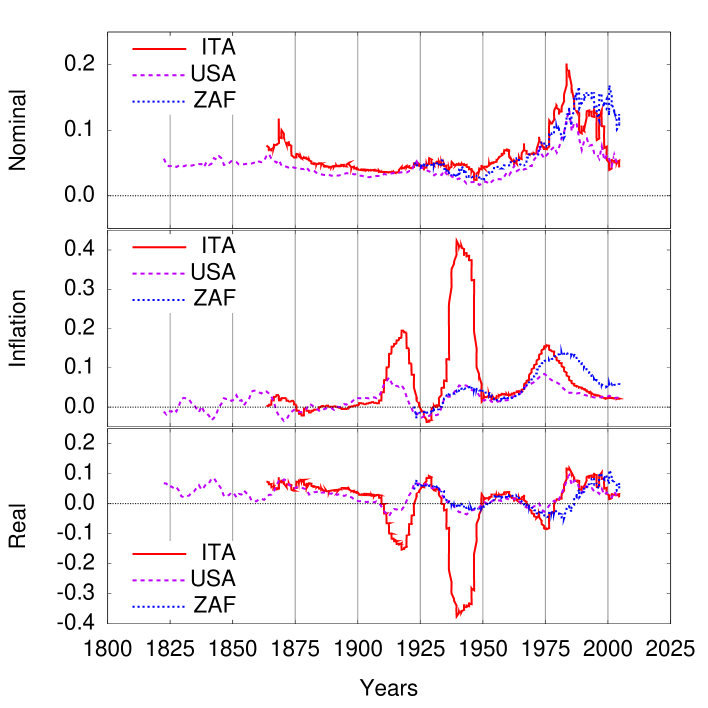
Figure 1: Real interest rates display large fluctuations and negative rates are not uncommon. We show nominal interest rates (top), inflation (middle), and real interest rates (bottom) for Italy (ITA), United States (USA) and South Africa (ZAF).

III Choosing the Ornstein-Uhlenbeck model

A striking feature observed in many epochs for all countries is that real interest rates frequently become negative, often by substantial amounts and for long periods of time (see Fig. 1 and Table 2). This rules out most standard financial models, which assume that interest rates are always positive Brigo2006 . We thus focus our attention on one of the three most popular stochastic models and on the only one that allows for negative rates: the Ornstein-Uhlenbeck model Uhlenbeck1930 , also known in the financial and economics literature as the Vasicek model vasicek and which is also being used for modelling market volatility Perello2003 ; Masoliver2002 ; Perello2004 ; Masoliver2006 . The model can be written as farmer2015

$$dr(t)=-\alpha(r(t)-m)dt+kdw(t),$$ (3)

where $r(t)$ is the real interest rate and $w(t)$ is a Wiener process, a Gaussian process with zero mean and unit variance. The parameter $m$ is a mean value to which the process reverts and coincides with the long-term average of the process (3) :

$$\mathbb{E}[r(t)]\simeq m.$$ (4)

The parameter $k$ is expressing the amplitude of the fluctuations and it is related to the variance which in the long-term limit reads

$$\mbox{Var}\left[r(t)\right]\simeq\frac{k^{2}}{2\alpha}.$$ (5)

The parameter $\alpha$ is the strength of the reversion to the mean $m$. The autocorrelation function in its long-term limit is

$$K(t-t^{\prime})=\mathbb{E}\left[(r(t)-m)(r(t^{\prime})-m)\right]\simeq\frac{k^{2}}{2\alpha}e^{-\alpha|t-t^{\prime}|},$$ (6)

where $\alpha^{-1}$ is the correlation time $\tau_{c}$ as can be seen from the definition

$$\tau_{c}\equiv\frac{1}{K(0)}\int_{0}^{\infty}K(\tau)d\tau=\frac{1}{\alpha}.$$

Table 2: Negative rates frequency. “Negative RI” and “Years” give respectively the time ratio and the number of years in which real interest rates are negative. The last row shows the average over all countries.

Country	Negative RI	Years
Argentina	0.20	17
Australia	0.23	33
Canada	0.22	20
Chile	0.56	43
Denmark	0.18	33
Germany	0.14	25
Italy	0.28	40
Japan	0.33	26
Netherlands	0.17	33
South Africa	0.43	36
Spain	0.25	45
Sweden	0.28	38
United Kingdom	0.14	45
United States	0.19	37
All countries	0.26	34

Recall that the OU model may attain negative rates. Let us quantify this characteristic by evaluating the probability $P(r<0,t|r_{0})$, for $r(t)$ to be negative. In the long-term limit we denote this probability by $P_{s}^{(-)}$, that is,

$$P_{s}^{(-)}=\lim_{t\rightarrow\infty}P(r<0,t|r_{0}).$$

For the OU model we have

$$P_{s}^{(-)}=\frac{1}{2}{\rm Erfc}\left(\mu/\kappa\right),$$ (7)

where ${\rm Erfc}(x)$ is the complementary error function expressed in terms of

$$\mu=\frac{m}{\alpha},\qquad\kappa=\frac{k}{\alpha^{3/2}}.$$ (8)

The dimensionless parameters $\mu$ and $\kappa$ are related to the average $m$ and the noise intensity $k$, respectively. As we will see later, these parameters provide a rather convenient way of describing important features about the discount function $D(t)$. In Fig. 2, we represent Eq. (7) and show the different values that the function $P_{s}^{(-)}$ can attain in terms of $\mu$ and $\kappa$.

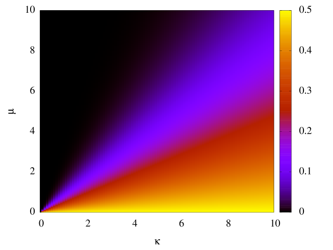
Figure 2: The probability of negative rates as given in Eq. (7). In the vicinity of the bottom right corner the probability of negative rates is around $0.5$ while at the upper left corner this probability is exponentially small and rates are mostly positive.

Using standard asymptotic expressions of ${\rm Erfc}(x)$ we can also get the behavior of $P_{s}^{(-)}$ in the cases (i) $\mu<\kappa$ and (ii) $\mu>\kappa$.

(i) When the normal rate $\mu$ is smaller than the volatility of the rate $\kappa$, we can use the series expansion

$${\rm Erfc}(z)=1-\frac{2}{\sqrt{\pi}}z+O(z^{2}).$$

Hence,

$$P_{s}^{(-)}=\frac{1}{2}-\frac{1}{\sqrt{\pi}}(\mu/\kappa)+O(\mu^{2}/\kappa^{2}).$$ (9)

For $\mu/\kappa$ sufficiently small, this probability approaches $1/2$. In other words, rates are positive or negative with almost equal probability. Note that this corresponds to a rather stressed situation in which noise $\kappa$ dominates over the mean value $\mu$.

(ii) When fluctuations around the normal level are smaller than the normal level itself, $\kappa<\mu$, we can use the asymptotic approximation

$${\rm Erfc}(z)\sim\frac{e^{-z^{2}}}{\sqrt{\pi}z}\left[1+O\left(\frac{1}{z^{2}}\right)\right],$$

and

$$P_{s}^{(-)}\sim\frac{1}{2\sqrt{\pi}}\left(\frac{\kappa}{\mu}\right)e^{-\mu^{2}/\kappa^{2}}.$$ (10)

Therefore, for mild fluctuations around the mean the probability of negative rates is exponentially small.

When $\kappa=\mu$, the probability of negative rates is $P_{s}^{(-)}=0.079$. Due to the ergodic character of the OU process Masoliver2018 , this means that when noise is balanced by the mean value (that is, $\kappa=\mu$), one may expect to have negative real rates $7.9\ \%$ of the time farmer2015 .

IV Discount function and negative rates for the Ornstein-Uhlenbeck model

It is possible to derive the exact expression for the discount function $D(t)$ defined in Eq. (1) in the case of the time-dependent OU model. As thoroughly described in Ref. farmer2015 , we write this expression in the form

$$\ln D(t)= - \left(m-\frac{k^{2}}{2\alpha^{2}}\right)t$$ (11)

$$+ \frac{1}{\alpha}\left[m-r_{0}-\frac{k^{2}}{4\alpha^{2}}\left(3-e^{-\alpha t}\right)\right]\left(1-e^{-\alpha t}\right).$$

The best way to study the discount rate is to work with the dimensionless time unit $\tau=\alpha t$, for afterwards focussing on the long-term limit $\tau\gg 1$ since climate action is primarily interested in this asymptotic value. Thus, as $\tau\to\infty$, the exact expression (11) shows at once that the discount function of the OU model decays exponentially

$$D(t)\simeq e^{-r_{\infty}t},$$ (12)

where (cf. Eq. (8))

$$r_{\infty}=m-k^{2}/2\alpha^{2}=\alpha\left(\mu-\kappa^{2}/2\right).$$ (13)

We see from this expression that the long-run discount rate $r_{\infty}$ is always lower than the average interest rate $m$, by an amount that depends on the dimensionless noise parameter $\kappa$. The long-run discount rate can therefore be much lower than the mean, and indeed can correspond to low interest rates that are rarely observed. This clearly illustrates the imprudence of assuming that the average real interest rate is the correct long-run discount rate.

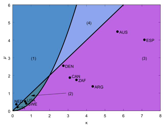
Figure 3: The four different scenarios for the discount with the cases of nine countries. The vertical axis is the dimensionless mean interest rate $\mu$ and the horizontal axis is the dimensionless fluctuation amplitude $\kappa$. Points correspond to nine of the fourteen countries presented and does not include the errors associated (cf. Table 4). The errors are important as can be seen in Table 4. Five countries are not reported here because they are far out of the range herein provided.

The long-run behavior of the discount rate (13) depends on the two dimensionless parameters $\mu$ and $\kappa$ (cf. Eq. (8)). The parameter space can be therefore divided into four regions, as shown in Fig. 3. In the region (1), where $\mu>\kappa^{2}/2$ (or equivalently $m>k^{2}/2\alpha^{2}$) and $\mu>\kappa$, the mean interest rate is large in comparison to the noise and negative rates are very infrequent. The long-run discounting function decays exponentially with rate $r_{\infty}>0$. In the region (2), albeit small, the long-run discounting function still decays exponentially with rate $r_{\infty}>0$ but negative rates are more frequent than $7.9\%$. Region (3) represents the most catastrophic situation since $\mu<\kappa^{2}/2$ and thus $r_{\infty}<0$, meaning that the discount function $D(t)$ increases exponentially and negative rates are rather frequent. Region (4) also shows $r_{\infty}<0$ although, in this case, it is mostly because the noise component is very intense and not due to the presence of a relevant frequency of negative return events. Finally, at the boundary $\mu=\kappa^{2}/2$, the long-run interest rate $r_{\infty}=0$ and the discount function is asymptotically constant.

V Estimating the discount function for the Ornstein-Uhlenbeck model

Table 3: Maximum Likelihood Estimation for the Ornstein-Uhlenbeck process described and the long-run interest rate. Countries have been reordered based on their estimated $\hat{r}_{\infty}$. $\hat{m}$ is the estimator of the mean real interest rate in 1/years. $\hat{\alpha}$ is the estimator related to the characteristic reversion time in 1/year. The squared root of the estimator of $k^{2}$ is the volatility of the process and $k^{2}$ is given in terms of $1/\mbox{(year)}^{3}$. These estimators are accompanied with the square root of the variance, $\sigma$’s, of each estimator. $\hat{r}_{\infty}$ is the subsequent estimator of the long-run real interest rate in 1/year. Negative values of $\hat{r}_{\infty}$ mean the discount function is asymptotically increasing and its standard error is obtained through error propagation. The last two rows show separately the average over all countries, the stable countries with $r_{\infty}>0$ and the unstable countries with $r_{\infty}<0$. In all three rows standard error provided corresponds to the standard deviation of the $\hat{r}_{\infty}$ for the different countries.

Country	$\hat{m}$	$\sigma_{\hat{m}}$		$\hat{\alpha}$	$\sigma_{\hat{\alpha}}$		$\hat{k^{2}}$	$\sigma_{\hat{k^{2}}}$		$\hat{r}_{\infty}$	$\sigma_{\hat{r}_{\infty}}$
Germany	-0.0945	0.6695		0.0071	0.0089		41.72E-04	2.19E-04		-40.94	2.28
Chile	-0.0579	0.3146		0.0201	0.0227		31.07E-04	2.49E-04		-3.917	0.442
Japan	0.0502	0.2468		0.0053	0.0114		13.96E-05	1.09E-05		-2.431	0.314
Italy	0.0197	0.1595		0.0056	0.0089		11.46E-05	0.68E-05		-1.778	0.192
Spain	0.0671	0.0692		0.0167	0.0137		23.71E-05	1.26E-05		-0.3578	0.0728
Argentina	0.0315	0.0709		0.0228	0.0231		22.40E-05	1.71E-05		-0.1831	0.0727
Australia	0.0397	0.0450		0.0089	0.0112		2.23E-05	0.13E-05		-0.1029	0.0458
South Africa	0.0269	0.0472		0.0154	0.0193		4.35E-05	0.34E-05		-0.0649	0.0477
Canada	0.0266	0.0391		0.0142	0.0178		2.75E-05	0.21E-05		-0.0415	0.0394
Denmark	0.0410	0.0259		0.0161	0.0133		3.15E-05	0.17E-05		-0.0197	0.0261
Sweden	0.0279	0.0166		0.0676	0.0317		16.92E-05	2.06E-05		0.0095	0.0167
USA	0.0319	0.0123		0.0603	0.0257		10.03E-05	1.05E-05		0.0181	0.0124
UK	0.0342	0.0062		0.1635	0.0326		31.37E-05	2.53E-05		0.0283	0.0062
Netherlands	0.0599	0.0078		0.1648	0.0550		17.97E-05	2.43E-05		0.0566	0.0078
All countries	0.0217	0.1236		0.0420	0.0211		63.45E-05	4.31E-05		-3.552	0.255
Stable	0.0385	0.0107		0.1140	0.0362		19.07E-05	2.02E-05		0.0281	0.0108
Unstable	0.0150	0.1686		0.0132	0.0150		81.20E-05	5.23E-05		-4.984	0.353

Table 4: Dimensionless mean interest rate and fluctuation amplitude for all countries. The dimensionless mean interest rate estimator $\hat{\mu}$ is accompanied with its error obtained through error propagation (cf. Eq. (8)) and by considering the parameters estimated and provided in Table 3. The dimensionless fluctuation amplitude estimator $\hat{\kappa}$ is accompanied with its standard error obtained through error propagation (cf. Eq. (8)) and by considering the parameters estimated and provided in Table 3.

Country	$\hat{\mu}$	$\sigma_{\hat{\mu}}$			$\hat{\kappa}$	$\sigma_{\hat{\kappa}}$
Germany	-13.22	95.11			106.92	198.75
Chile	-2.89	16.01			19.61	33.26
Japan	9.46	50.79			30.59	98.70
Italy	3.49	28.79			25.23	59.94
Spain	4.02	5.30			7.13	8.79
Argentina	1.38	3.40			4.34	6.58
Australia	4.48	7.61			5.67	10.77
South Africa	1.75	3.77			3.45	6.50
Canada	1.88	3.62			3.10	5.83
Denmark	2.55	2.65			2.75	3.41
Sweden	0.41	0.31			0.74	0.52
USA	0.53	0.30			0.68	0.43
UK	0.21	0.06			0.27	0.08
Netherlands	0.36	0.13			0.20	0.10
All countries	1.03	15.56			15.05	30.99
Stable	0.39	0.20			0.47	0.28
Unstable	1.29	21.71			20.89	43.25

We now estimate the parameters $m$, $k$ and $\alpha$ together with the dimensionless parameters $\mu$ and $\kappa$ defined in Eq. (8). We perform such an estimation for each historical series (cf. Table 1) by using a well-established maximum likelihood procedure for the OU model Brigo2006 . The resulting estimators $\hat{m}$, $\hat{\alpha}$, and $\hat{k^{2}}$ are listed in Table 3 along with their standard deviation derived from formulas provided in Ref. Chen2009 . Table 3 shows that the most inaccurate estimator is $\hat{\alpha}$, a not surprising fact since the estimation of $\alpha$ is quite a challenge in any Ornstein-Uhlenbeck process Chen2009 . The last two columns in Table 3 include the long-run interest rate estimator $\hat{r}_{\infty}$ and its error calculated through error propagation.

We can also observe the position $(\hat{\kappa},\hat{\mu})$ of each country in Fig. 3 by considering the results presented in Table 4. In any case these results need to be understood as a first-order approximation since the errors behind the estimators (which are evaluated through error propagation) are significant (see Table 4). Only four countries show a positive long-run rate, $r_{\infty}>0$, and all of them inside, or very close, to the region defined by $\mu<\kappa$ in which rates are frequently negative. The other ten countries show less stable behavior and are all of them in the exponentially increasing region (Region 3), which implies they have long-run negative rates, and are widely scattered. In two cases (Germany and Chile) the average rate $m$ (and its dimensionless version $\mu$) is negative due to at least one period of runaway inflation while two others (Japan and Italy) still have a long-run negative rate $r_{\infty}$ mostly due to a very small strength of the reversion to the mean given by the parameter $\alpha$ (cf. Eq. (3)). These four countries are not plotted in Fig. 3 because they are out the range of $\mu$ and/or $\kappa$ axis.

Also note that all fourteen countries but one (Netherlands) are below the identity line, $\mu=\kappa$, in Fig 3 which indicates that negative real interest rates are common (even in the stable countries they occur $20\%$ of the time). It is also worth to mention that only one is above Nordhaus’s 4$\%$ discounting rate Nordhaus (5.7$\%$, Netherlands) and only two more countries are above the more pessimistic discounting rate (1.4$\%$) provided by Stern Stern (1.8$\%$ and 2.8$\%$ from USA and United Kingdom, respectively). And more generally, it is important to notice that $r_{\infty}$ is very much smaller than $m$ in most of the cases. All these statements are robust even when considering values of the estimators with shifts of the size of its standard error (see Table 3).

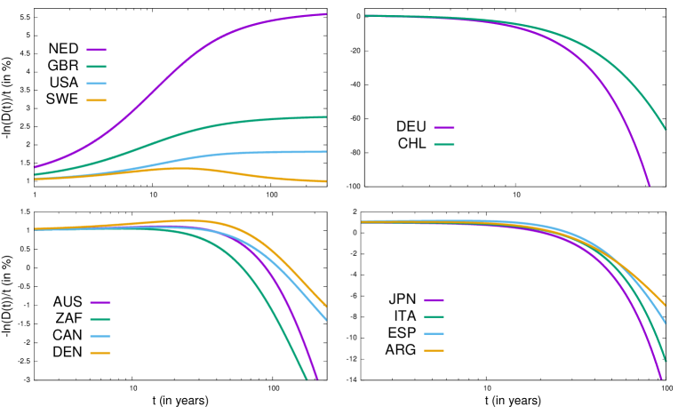
Figure 4: The logarithmic discounting rate (in percent) as a function of time (in years). We have divided the countries in four groups to represent Eq. (11) with parameters provided in Table 4 and taking $r_{0}=1\%$.

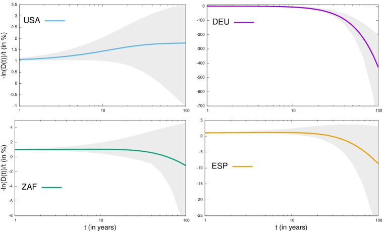
Figure 5: The logarithmic discounting rate (in percent) and its error as a function of time (in years). We have selected four countries (from each of the four groups provided in Fig. 4: United States, Germany, South Africa, and Spain) to represent Eq. (11) by taking $r_{0}=1\%$. Grey shadow considers a range limited by minimum and maximum values when adding to each parameter the impact of their standard error to the value of the discount rate as a function of time. Parameters and their standard error are both provided in Table 3.

The characteristic (correlation) time ($\tau_{c}=1/\alpha$) for each country appears to be very different (cf. Table 3). Some countries must spend more than a century to achieve a stationary level and thus finally attain the long-run discount rate $r_{\infty}$. Furthermore, this time horizon might be even larger than the time interval we must consider to make a response, from an economic point of view, to any climate change catastrophe. For this reason, it is interesting to investigate how the discount rate defined as $-\ln(D(t))/t$ changes over time (cf. Eq. (11)).

Figure 4 shows the discount rates for all countries as a function of time by considering initial rate $r_{0}=1\%$ which clearly illustrates the dramatic differences between countries. In this way we divide the fourteen countries into roughly four groups. There are two countries (DEU, CHL) that show a very fast and very negative rate. There is a second group still having a monotonic behavior but with a much slower trend to raise negative discount rates (JPN, ITA, ESP and ARG). Non-monotonic behavior is indeed observed in a third group (AUS, ZAF, CAN, DEN). This group is of special interest since it shows how the rates might first grow by finally becoming negative after 20 or 30 years. Stable countries represented in the first inset on the left of Fig. 4 also show that the asymptotic rate $r_{\infty}$ is raised very slowly being the country with the highest rate (NED) the one that needs more than a century to attain the stationary level. Figure 5 selects four countries (USA, DEU, ZAF and ESP), one from each of the groups mentioned above, to observe the impact of uncertainty as a function of time. For different values of time, the discount function includes a shadow in grey limited by maximum and minimum values when taking into consideration the standard error of each of the estimators. In all four countries and at any time, maximum discount rate value is always below 2.2%. The inclusion of the statistical uncertainty reinforces the robustness of our results.

Let us finally note that these results are in contrast to other treatments of fluctuating rates which assume that short term rates are positive and predict that the decrease in the discounting rate occurs over a much longer timescale, usually measured in hundreds or thousands of years Weitzman98 ; NewellPizer ; Groom ; Farmer ; Hepburn ; Freeman ; GollierBook .

VI Considering alternative models

As mentioned above the Ornstein-Uhlenbeck model is the only one among the three most classic models allowing for negative rates. This is the reason why we have excluded both the Feller and the lognormal models from our analysis. Let us nonetheless briefly study what modifications should be carried out in order to use these positive rate models in our analysis.

VI.1 The shifted Feller model

The Feller process Feller1951 (see also Masoliver2018 ) has a very similar structure than the Ornstein-Uhlenbeck process except that the noise component depends on the interest rate. The process also has a mean reverting force that makes the process have an autocorrelation function that decays in an exponential manner whose characteristic time scale is $1/\alpha_{F}$. Let us however remind that Feller does not allow for negative rates and these are clearly present in our empirical data. Therefore, to consider the Feller process for estimating the long-run discount rate $r_{\infty}$ would require to redefine the Feller model that reads

$$dy(t)=-\alpha_{F}(y(t)-m_{F})dt+k_{F}\sqrt{y(t)}dw(t),$$ (14)

where

$$y=r-r_{min}$$ (15)

and $r_{min}<0$ is the minimum value observed in the time series. The estimation through maximum likelihood procedure and its error analysis is also possible Chen2009 . Table 5 compares the Ornstein-Uhlenbeck and the shifted Feller models which have very similar mathematical expressions for estimating $\hat{m}$, $\hat{\alpha}$ and $\hat{k}^{2}$ parameters. The discount function now reads (cf. Eqs. (1)) and (15))

$$D(t)=\mathbb{E}\left[\exp{\left(-\int_{0}^{t}\left(r_{min}+y(t^{\prime})dt^{\prime}\right)\right)}\right]=\exp\left(-r_{min}t\right)\mathbb{E}\left[\exp{\left(-\int_{0}^{t}y(t^{\prime})dt^{\prime}\right)}\right].$$

The asymptotic value of the remaining average shows an exponential decay farmer2015

$$\mathbb{E}\left[\exp{\left(-\int_{0}^{t}y(t^{\prime})dt^{\prime}\right)}\right]\simeq e^{-y^{F}_{\infty}t},$$

whose long-run discount rate farmer2015 is

$$y^{F}_{\infty}=\frac{2m_{F}}{1+\sqrt{1+2k_{F}^{2}/\alpha_{F}^{2}}},$$

so that

$$D(t)=e^{-\left(r_{min}+y^{F}_{\infty}\right)t}=e^{-r^{F}_{\infty}t}.$$

We observe that (as in the Ornstein-Uhlenbeck process) the log-run rate is smaller than the average rate, $r^{F}_{\infty}<m$. However, the shifted Feller process leads us to obtain a slightly larger estimation but within the statistical error range ($3.4\%$ versus $1.81\%$, see Table 5). The value is similar than Nordhaus’s $4\%$ discounting rate if one considers the statistical error and in any case lower than $6\%$ Nordhaus ; Nordhaus2007 .

Table 5: Maximum Likelihood Estimation for the three different models described and the long-run interest rate for the case of United States. These estimators are taking years as a basic time unit and they are all accompanied with the square root of the variance, $\sigma$’s, of each estimator. $\hat{r}_{\infty}$ is the subsequent estimator of the long-run real interest rate in 1/year. For the Feller and lognormal cases we have provided a modified version of the model (cf. Eqs. (14) and (16)). The shifted Feller and lognormal models takes $r_{min}=-0.0415$, which is its minimum value in the historical time series, and the estimated $\hat{r}_{\infty}$ is corrected by adding $r_{min}$ but this has been impossible to be done in the lognormal case since the asymptotic value goes to a constant.

	$\hat{m}$	$\sigma_{\hat{m}}$		$\hat{\alpha}$	$\sigma_{\hat{\alpha}}$		$\hat{k}^{2}$	$\sigma_{\hat{k}^{2}}$		$\hat{r}_{\infty}$	$\sigma_{\hat{r}_{\infty}}$
Ornstein-Uhlenbeck	0.0319	0.0123		0.0603	0.0257		10.03E-05	1.05E-05		0.0181	0.0124
	$\hat{m}_{F}$	$\sigma_{\hat{m}_{F}}$		$\hat{\alpha}_{F}$	$\sigma_{\hat{\alpha}_{F}}$		$\hat{k}_{F}^{2}$	$\sigma_{\hat{k^{2}}_{F}}$		$\hat{r}^{F}_{\infty}$	$\sigma_{\hat{r}^{F}_{\infty}}$
Shifted Feller	0.0864	0.0041		0.0599	0.0057		12.56E-05	1.31E-05		0.0349	0.0072
	$\hat{m}_{L}$	$\sigma_{\hat{m}_{L}}$		$\hat{k}_{L}^{2}$	$\sigma_{\hat{k}_{L}^{2}}$		$\hat{m}_{L}-\hat{k}_{L}^{2}/2$	$\sigma_{\hat{m}_{L}-\hat{k}_{L}^{2}/2}$		Asymp
Shifted lognormal	0.0130	0.0163		0.0309	0.0066		-0.0024	0.0130		constant

VI.2 The shifted lognormal model

Another alternative to still allow for negative rates is to consider a modified version of the lognormal process by considering new variable $y=r-r_{min}$ (where $r_{min}<0$ is the minimum value observed in the time series) and the following stochastic dynamics:

$$dy(t)=m_{L}y(t)dt+k_{L}y(t)dw(t),$$ (16)

whose long-run discount function can lead to three different asymptotic expressions farmer2015 :

$$\mathbb{E}\left[\exp{\left(-\int_{0}^{t}y(t^{\prime})dt^{\prime}\right)}\right]\sim\begin{cases}\mathrm{constant}&\quad m_{L}<k_{L}^{2}/2,\\ e^{-y^{L}_{\infty}t}&\quad m_{L}>k_{L}^{2}/2.\\ t^{-1/2}&\quad m_{L}=k_{L}^{2}/2,\end{cases}$$

For the exponential case the long-run discount rate reads

$$y^{L}_{\infty}=\frac{m_{L}-k^{2}_{L}/2}{\psi\left(2m_{L}/k_{L}^{2}\right)+1/(2m_{L}/k_{L}^{2}-1)},$$

where $\psi(\cdot)$ is the digamma function. The lognormal process does not show any reversion trend to a certain level and its average grows (or decreases) in an exponential manner

$$\mathbb{E}\left[r(t)|r(0)=r_{0}\right]=(r_{0}+r_{min})e^{m_{L}t}-r_{min},$$

a result that it is in contradiction with the times series provided in Fig. 1. We can however also estimate the parameters via maximum likelihood procedures. The results are again provided in Table 5 and they show us that the asymptotic discount falls into the constant case since $m_{L}<k_{L}^{2}/2$ although the error analysis warn us that we cannot discard the exponential case (being not greater $4-5\%$) nor the hyperbolic slow decay.

VI.3 Extending the Ornstein-Uhlenbeck process

One can argue that the results presented can change under different historical conditions or periods. To exemplify this issue, we have also estimated these values in the case of Germany once the World War II was over (from March 1946). Parameters are in that case $\mu=0.62$, $\kappa=0.32$ with now a positive long-run rate $r_{\infty}=3.4\%$ which is in any case smaller than Nordhaus estimates for valuing climate action Nordhaus2007 . Germany certainly is a quite volatile situation challenging the model which assumes constant (i.e., stationary) parameters. A possible way out is to extend the model with an additional dimension under the form of a “matrioshka doll” by considering $m$ as a stochastic process following an additional Ornstein-Uhlenbeck process Perello2004

$$dr=-\alpha(r-m)dt+kdw(t)$$

$$dm=-\alpha_{0}(m-m_{0})dt+k_{0}dw_{0}(t),$$ (17)

where the Wiener processes $w(t)$ and $w_{0}(t)$ are both zero mean, have unit variance and are independent from each other implying that $\mathbb{E}\left[dw(t)dw_{0}(t)\right]=0$. We also assume that $\alpha>\alpha_{0}>0$ thus showing a slower mean reverting force for the subordinated process $m_{0}$ than for $m$. A similar extension has been used in other financial contexts to model stochastic volatility Perello2004 by adding a longer mean reversion process which allows for a slow decaying memory for the volatility process while still preserving a much shorter memory for the so-called leverage effect Masoliver2006 ; Perello2003 (see also Ref. Delpini2015 for another setting that could represent an alternative approach to the extended Ornstein-Uhlenbeck model given by Eq. (17)). In the long-run, the process reads Perello2004 :

$$m(t) = m_{0}+k_{0}\int_{-\infty}^{t}e^{-\alpha_{0}(t-t^{\prime})}dw_{0}(t)$$

$$r(t) = m_{0}+k\int_{-\infty}^{t}e^{-\alpha(t-t^{\prime})}dw(t)+\frac{k_{0}}{\alpha-\alpha_{0}}\int_{-\infty}^{t}\left(e^{-\alpha_{0}(t-t^{\prime})}-e^{-\alpha(t-t^{\prime})}\right)dw_{0}(t).$$ (18)

We can easily see that this extended process shows the same average, $\mathbb{E}\left[r(t)\right]=m_{0}$, than the simpler OU version but with greater variance (cf. Eqs. (4) and (5), respectively)

$${\rm Var}[r(t)]=k^{2}/2\alpha+k_{0}^{2}/2\alpha_{0}$$ (19)

The autocorrelation function now reads Perello2004 (cf. Eq. (6)):

$$K(t-t^{\prime}) = \mathbb{E}\left[(r(t)-m_{0})(r(t^{\prime})-m_{0})\right]$$

$$= \left(\frac{k^{2}}{2\alpha}-\frac{k_{0}^{2}\alpha}{2(\alpha^{2}-\alpha_{0}^{2})}\right)e^{-\alpha|t-t^{\prime}|}+\frac{k_{0}^{2}\alpha^{2}}{2(\alpha^{2}-\alpha_{0}^{2})\alpha_{0}}e^{-\alpha_{0}|t-t^{\prime}|},$$

where the first term with an exponential decay with $1/\alpha$ would dominate for short time difference $|t-t^{\prime}|$. In the opposite situation, for longer time difference, the second exponential decay expressed in terms of $1/\alpha_{0}$ would dominate. The extended process now have five parameters ($\alpha,k,\alpha_{0},k_{0}$, and $m_{0}$), while basic OU process had only three ($\alpha,k$, and $m$).

We can finally look at the effects on the asymptotic discount. It can be in this case proved that the process has also an exponential decay with a long-run discount rate that reads Masoliver2020

$$r_{\infty}^{ext}=m_{0}-\frac{1}{2}\left(\frac{k^{2}}{2\alpha^{2}}+\frac{k_{0}^{2}}{2\alpha_{0}^{2}}\right).$$ (20)

The result brings rates which are even lower than the one provided by the maximum likelihood estimation procedure in the simple Ornstein-Uhlenbeck process. As a simple exercise we can estimate a combination of $k_{0}$ and $\alpha_{0}$ with the historical variance of the whole process (see Eq. (19)). To estimate $\alpha_{0}$ is not that simple since our historical data sets are too short and its estimation becomes too noisy. However, jointly with the values already obtained for Orstein-Uhlenbeck maximum likelihood estimation for $m$ (now equivalent to $m_{0}$), $k$, and $\alpha$, it is possible to observe the effects for different values of $\alpha_{0}$:

$$r_{\infty}^{ext}=m_{0}-\frac{1}{2}\left[\frac{k^{2}}{2\alpha^{2}}+\left({\rm Var}(r(t))-\frac{k^{2}}{2\alpha}\right)\frac{1}{\alpha_{0}}\right].$$

In this case we can see that the long-run rate $r_{\infty}$ for the United States is practically zero when $\alpha_{0}=\alpha/20$.

VII Discussion

Our empirical analysis proves that real interest rates are often negative –roughly a quarter of the time– which implies that one must use a discount model that is compatible with this property. For this purpose we have proposed the Ornstein-Uhlenbeck model which has the additional advantage that it can be solved analytically in a relatively simple way. This model facilitates the understanding of why the long-run discount rate can be so low. A first reason is that real interest rates are themselves typically low. As we have showed the average over all countries surveyed is negative, and even the average over stable countries (those with a positive long-run rate, $r_{\infty}>0$) is $2.8\%$. A second reason is that the fluctuating part on the right hand side of Eq. (13), which depends both on the noise intensity $k$ and the persistence term $1/\alpha$, typically lowers rates for the stable countries by about $7\%$. In some cases, such as Spain, the effect is much more dramatic: Even though the mean short term rate has the high value of $m=6.7\%$, the long-term discounting rate is $r_{\infty}=-36\%$ which would imply a great increasing discount. The estimation is being done with a maximum likelihood procedure that includes an error analysis that demonstrates the robustness of the results obtained.

Our analysis here makes several simplifications such as ignoring non-stationarity. We have here partially address this issue by extending the Ornstein-Uhlenbeck which allows for slower fluctuations in the normal level and resulting even in lower long-run discount rates Masoliver2020 . Correlations between the environment and the economy have also being ignored but, in any case, despite the variety of results, the long-run discount rate is always smaller than Nordhaus estimates by other methods as we have exemplified with the German case Nordhaus2007 . We have also not considered the market price of risk vasicek ; masoliver_2018(b) , in other words, we have assumed that markets are risk neutral and the average in Eq. (1) defining the discount function, is evaluated using the empirical probability measure without any risk adjustment cox_81 ; piazzesi . These issues are under present investigation and some results are expected soon farmer2020 .

In any case the methods that we have introduced here provide a foundation on which to incorporate more realistic assumptions. We do not mean to imply that it is realistic to actually use the increasing discounting functions that occur for countries with less stable interest rate processes. There is some validity to treating hyper-inflation as an aberration – when it occurs government bonds are widely abandoned in favor of more stable carriers of wealth such as land and gold, and as a result under such circumstances the difference between nominal interest and inflation may underestimate the actual real rate of interest.

Nonetheless, real interest rates are closely related to economic growth, and economic downturns are a reality. The great depression lasted for 15 years, and the fall of Rome triggered a depression in western Europe that lasted almost a thousand years. In light of our results here, arguments that we should wait to act on global warming because future economic growth will easily solve the problem should be viewed with extreme skepticism. Our analysis clearly supports Stern over Nordhaus. When we plan for the future we should always bear in mind that sustained economic downturns may visit us again, as they had in the past.

Effective responses to this multifaceted problem have been slow to develop, in large part because many experts have not only underestimated its impact, but also overlooked the underlying institutional structure, organizational power and financial roots Stern2016 ; Farrell2019 . A growing body of sophisticated research is currently emerging with a large set of multidisciplinary strategies that wants to exploit socioeconomic tipping points (as in any complex dynamical system) to magnify the impact of each political intervention Farmer2019 and also integrate science-policy perspectives with public awareness, citizen-led research and citizen science practices (see for instance Vicens2019 ; Kythreotis2019 ). In all cases the final purpose is to better respond to global challenges such as climate action in a near future, sooner rather than later.

Acknowledgements

We thank to an anonymous referee for the several comments that have allowed to improve the final version of the paper. We also would like to thank National Science Foundation grant 0624351 (JG) and the Institute for New Economic Thinking (JDF). This work was supported by MINECO (Spain) FIS2013-47532-C3-2-P (JM, MM and JP), FIS2016-78904-C3-2-P (JM, MM and JP); by Generalitat de Catalunya (Spain) through Complexity Lab Barcelona (contract no. 2017 SGR 1064, JM, MM and JP)

References

- (1) Mantegna R N and Stanley H E, 1999 Introduction to econophysics: correlations and complexity in finance (Cambridge University Press, Cambridge)
- (2) Bardoscia M, Livan G and Marsili M, Statistical mechanics of complex economies, 2017 Journal of Statistical Mechanics: Theory and Experiment 2017(4) 043401.
- (3) Bouchaud J P, Econophysics: still fringe after 30 years?, 2019 Europhysics News 50(1) 24-27.
- (4) Farmer J D, Patelli P and Zovko I I, The predictive power of zero intelligence in financial markets 2005 Proceedings of the National Academy of Sciences 102(6) 2254-2259
- (5) Dall’Amico L, Fosset A, Bouchaud J P and Benzaquen M, How does latent liquidity get revealed in the limit order book? 2019 Journal of Statistical Mechanics: Theory and Experiment 2019(1) 013404
- (6) Masoliver J and Perello J, A correlated stochastic volatility model measuring leverage and other stylized facts 2002 International Journal of Theoretical and Applied Finance 5(05) 541–562
- (7) Perelló J and Masoliver J, Random diffusion and leverage effect in financial markets 2003 Physical Review E 67(3) 037102
- (8) Perelló J, Masoliver J and Bouchaud J-P, Multiple time scales in volatility and leverage correlations: a stochastic volatility model 2004 Applied Mathematical Finance 11(1) 27–50
- (9) Perelló J, Masoliver J, Anento N, A comparison between several correlated stochastic volatility models 2004 Physica A: Statistical Mechanics and its Applications 344(1-2) 134-137
- (10) Masoliver J and Perelló J, Multiple time scales and the exponential Ornstein–Uhlenbeck stochastic volatility model 2006 Quantitative Finance 6(5) 423-433
- (11) Perelló J, Montero M, Palatella L, Simonsen I and Masoliver J, Entropy of the Nordic electricity market: anomalous scaling, spikes, and mean-reversion 2006 Journal of Statistical Mechanics: Theory and Experiment 2006(11) P11011
- (12) Perelló J, Sircar R, Masoliver J, Option pricing under stochastic volatility: the exponential Ornstein–Uhlenbeck model 2008 Journal of Statistical Mechanics: Theory and Experiment 2008(06) P06010
- (13) Camprodon, J., Perelló, J. Maximum likelihood approach for several stochastic volatility models 2012 Journal of Statistical Mechanics: Theory and Experiment 2012(08) P08016
- (14) Bormetti G, Cazzola V, Montagna G and Nicrosini O, The probability distribution of returns in the exponential Ornstein—Uhlenbeck model 2008 Journal of Statistical Mechanics: Theory and Experiment 2008(11) P11013
- (15) Delpini D and Bormetti G, Minimal model of financial stylized facts 2011 Physical Review E 83(4) 041111
- (16) Delpini D and Bormetti G, Stochastic volatility with heterogeneous time scales 2015 Quantitative Finance 15(10) 1597–1608
- (17) Samuelson P, A note on measurement of utility 1937 Rev Econ Stud 4 155–161
- (18) Dasgupta P, 2004 Human Well-Being and the Natural Environment (Oxford University Press, Oxford)
- (19) Stern N, 2006 The Economics of climate change: The Stern Review (Cambridge University Press, Cambridge)
- (20) Nordhaus W D, The Stern Review on the economics of climate change 2007 J Econ Literature 45 687–702.
- (21) Nordhaus W D, Critical assumptions in the Stern Review on Climate Change 2007 Science 317 201–202
- (22) Dasgupta P, The Stern Review’s economics of climate change 2007 National Institute Economic Review 199.1 4–7
- (23) Mendelsohn R O, A critique of the Stern Report 2006 Regulation 29 42
- (24) Weitzman M L, A review of the Stern review on the economics of climate change 2007 J Econ Literature 45 703–724
- (25) Nordhaus W D, 2008 A Question of Balance (Yale University Press, New Haven)
- (26) Stern N, 2015 Why Are We Waiting? The Logic, Urgency, and Promise of Tackling Climate Change (MIT Press, Massachussets)
- (27) The 2018 Report of the Global Commission on the Economy and Climate (The New Climate Economy, www.newclimateeconomy.report)
- (28) Arrow K J, Cropper M L, Gollier C, Groom B, Heal G M, Newell R G, Nordhaus W D, Pindyck R S, Pizer W A, Portney P R, Sterner T, Tol R S J, Weitzman M L, How should benefits and costs be discounted in an intergenerational context? The views of an expert panel (December 19, 2013) Resources for the Future 12–53
- (29) Chichilnisky G, Hammond P J, Stern N, Should We Discount the Welfare of Future Generations? Ramsey and Suppes versus Koopmans and Arrow 2018 University of Warwick, Department of Economics No. 1174
- (30) Weitzman M L, Why the far-distant future should be discounted at its lowest possible rate 1998 J Environment Econ and Management 36(3) 201–208
- (31) Gollier C, Koundouri P, Pantelidis T, Declining Discount Rates: Economic justifications and implications for long-run policy 2008 Economic Policy 23 757–795
- (32) Newell R, Pizer N, Discounting the Distant Future: How much do uncertain rates increase valuations? 2003 J Environ Econ and Management 46 52–71
- (33) Farmer JD, Geanakoplos J, Masoliver J, Montero M, Perelló J, Value of the future: Discounting in random environments 2015 Phys Rev E 91 052816
- (34) Groom B, Koundouri P, Panopoulou E, Pantelidis T, Discounting distant future: how much selection affect the certainty equivalent rate 2007 J Appl Econometrics 22 641–656
- (35) Hepburn C, Koundouri P, Panopoulou E, Pantelidis T, Social discounting under uncertainty: a cross-country comparison 2007 J Environ Econ and Management 57 140–150
- (36) Freeman M C, Groom B, Panopoulou E, Pantelidis T, Declining discount rates and the Fisher Effect: Inflated past, discounted future? 2015 J. Environ Econ and Management 73 32–49
- (37) Farmer J D, Geanakoplos J, Hyperbolic discounting is rational: Valuing the far future with uncertain discount rates 2009 Cowles Foundation Discussion Paper No. 1719. Available from: http://dx.doi.org/10.2139/ssrn.1448811
- (38) Uhlenbeck G E, Ornstein L S, On the theory of Brownian Motion 1930 Phys Rev 36 823-841
- (39) Feller W, Two singular diffusion processes 1951 Ann Math. 54 173-182
- (40) Osborne M F M, Brownian motion in the stock market 1959 Operation Research 7 145-173
- (41) Brigo D, Mercurio F, 2006 Interest Rate Models Theory and Practice (Springer-Verlag, Berlin and New York)
- (42) Vasicek O, An equilibrium characterization of the term structure 1977 J. Fin. Econ. 5 177-188
- (43) Masoliver J, 2018 Random Processes: First-passage and Escape (World Scientific, Singapore)
- (44) Tang C Y, Chen S X, Parameter estimation and bias correction for diffusion processes 2009 Journal of Econometrics 149(1) 65-81
- (45) Gollier C, 2012 Pricing the Planet Future: The Economics of Discounting in an Uncertain World (Princeton University Press, Princeton)
- (46) Masoliver J, Montero M, Perelló J, in preparation
- (47) See, for instance, Chapter 9 of Ref. Masoliver2018 for a plain and rather complete exposition
- (48) Cox J C, Ingersoll J E, Ross J A, A re-examination of the traditional hypothesis about the term structure of interest rates 1981 J. Finance 36 769-799
- (49) Piazzesi M, Affine term structure models In Sahala Y A, Hausen L P, 2009 (Eds.) The Handbook of Financial Econometrics (Elsevier, Netherlands, pp. 691-766)
- (50) Farmer J D, Geanakoplos J, Masoliver J, Montero M, Perelló J, Richiardi M G, Discounting the distant future: What do historical bond prices imply about the long term discount rate?, submitted for publication
- (51) Stern N, Economics: Current climate models are grossly misleading 2016 Nature 530 407–409
- (52) Farrell J, McConnell K, Brulle R, Evidence-based strategies to combat scientific misinformation 2019 Nature Climate Change 9 191-195
- (53) Farmer J D, Hepburn C, Ives M C, Hale T, Wetzer T, Mealy P, R. Rafaty R, Srivastav1 S, Way R, Sensitive intervention points in the post-carbon transition 2019 Science 364(6436) 132-134
- (54) Vicens J, Bueno-Guerra N, Gutiérrez-Roig M, Gracia-Lázaro C, Gómez-Gardenes J, Perelló J, Sánchez A, Moreno Y, Duch J, Resource heterogeneity leads to unjust effort distribution in climate change mitigation 2018 PLoS ONE 13(10): e0204369
- (55) Kythreotis A P, Mantyka-Pringle C, Mercer T G, Whitmarsh L E, Corner A, Paavola J, Chambers C, Miller B A, Castree N, Citizen Social Science for more integrative and effective climate action: a science-policy perspective 2019 Frontiers in Environmental Science 7 10