Wormholes in Poincarè gauge theory of gravity

Abstract

In the present work, we study static spherically symmetric solutions representing wormhole configurations in Poincarè gauge theory (PGT). The gravitational sector of the Lagrangian is chosen as a subclass of PGT Lagrangians for which, the spin-$0^{+}$ is the only propagating torsion mode. The spacetime torsion in PGT has a dynamical nature even in the absence of intrinsic angular momentum (spin) of matter, hence, torsion can play a principal role in the case of usual spin-less gravitating systems. We therefore consider a spin-less matter distribution with an anisotropic energy momentum tensor (EMT) as the supporting source for wormhole structure to obtain a class of zero tidal force wormhole solutions. It is seen that the matter distribution obeys the physical reasonability conditions, i.e., the weak (WEC) and null (NEC) energy conditions either at the throat and throughout the spacetime. We further consider varying equations of state in radial and tangential directions via definitions $w_{r}(r)=p_{r}(r)/\rho(r)$ and $w_{t}(r)=p_{t}(r)/\rho(r)$ and investigate the behavior of state parameters at the throat of wormhole. We observe that our solutions allow for wormhole configurations without the need of exotic matter. Observational features of the wormhole solutions are also discussed utilizing gravitational lensing effects. It is found that the light deflection angle diverges at the throat (which indeed, effectively acts as a photon sphere) and can get zero and negative values depending on the model parameters.

1 Introduction

One of the most fascinating features of general relativity (GR) that has attracted many researchers so far, is the possible existence of hypothetical geometries which have nontrivial topological structure, known as wormholes. The first attempt toward understanding the concept of wormhole was carried out by Ludwing Flamm in 1916 [1] where he noticed that the spatial part of the Schwarzschild spacetime describes something like a bridge or a shortcut between two worlds or two parts of the same world. However, it became clear that the wormhole solutions proposed by him are not traversable and hence are not relativistically applicable. In 1935, a specific wormhole-type solution was proposed by Einstein and Rosen [2]. Their motivation was to construct an elementary particle model represented by a “bridge structure” connecting two identical sheets. This solution was subsequently denoted as Einstein-Rosen bridge. The concept of traversable wormholes was firstly introduced by Misner and Wheeler through their pioneering works [3, 4], where these objects were obtained from the coupled equations of electromagnetism and GR and were denoted as “geons”, i.e., gravitational-electromagnetic entities [5]. Wheeler considered Reissner-Nordstrom or Kerr wormholes, as objects of the quantum foam, which connect different regions of spacetime and operate at the Planck scale. These objects were transformed later into Euclidean wormholes by Hawking [6] and others. However, the Wheeler wormholes were properly understood as non-traversable [7] wormholes, and additionally would, in principle, develop some type of singularity [8]. The simplest exact traversable wormhole solution was discovered in 1973 by Bronnikov [9] and independently by Ellis [10]. The wormhole throat for these solutions is supported by a phantom field which is a scalar field with negative kinetic energy. In a subsequent work, Ellis obtained the evolving version of his solution [11]. Also, Clement considered wormhole like solutions in higher dimensional GR [12], Einstein-Maxwell theory with an auxiliary scalar field [13] and Einstein-Yang-Mills theory with a ghost Higgs field [14], see also [15, 16] for overviews of wormhole research. However, the interest in wormhole physics was highly stimulated in 1988 after the pioneering work of Morris and Thorne who proposed a new idea of traversable wormhole [17, 18]. They investigated this issue through introducing a static spherically symmetric metric and discussed the required conditions for physically meaningful Lorentzian traversable wormholes. However, traversability of a wormhole requires inevitably the violation of null energy condition (NEC). In other words, the matter field providing this geometry is known as exotic matter for which the energy density becomes negative resulting in the violation of NEC [19]. Although the violation of energy conditions is unacceptable from the common viewpoint of physicists, it has been shown that some effects due to quantum field theory, e.g., Casimir effect can allow for such a violation [20]. Also, negative energy densities which are required to support the wormhole configuration may be produced through gravitational squeezing of the vacuum [21], see also [19, 22] for more details. However, it is generally believed that all classical forms of matter obey the standard energy conditions.

Researches on physics of wormholes by Morris, Thorne, and Yurtsever have opened up, in recent years, a new field of study in theoretical physics and several publications have appeared in recent years among which we can quote, traversable wormhole geometries constructed by matter fields with exotic EMT [23], phantom or quintom-type energy [24] and wormholes supported by nonminimal interaction between dark matter and dark energy [25], see [26] for a comprehensive review. Also an intriguing hypothesis concerns the possibility that the Milky Way could be a huge wormhole [27]. However, owing to the problematic nature of exotic matter, many attempts have been made toward minimizing its usage and in this way, modified gravity theories [28], as extensions of GR, can provide a setting in order to overcome the issue of energy conditions for wormhole structures. Much research on wormhole solutions in modified gravity has been done including, wormholes in the framework of gravitational decoupling [29], Lovelock theories [30], Rastall gravity [31], modified gravities with curvature-matter coupling [32], scalar-tensor theory [33], $f({\sf R})$ gravity [34], Einstein-Cartan theory (ECT) [35, 36], Einstein-Gauss-Bonnet [37] and other theories [38].

An important issue that motivates one to seek for possible generalizations of GR is to provide a correct basis for involving intrinsic angular momentum (spin) of gravitating sources along with suitable conservation laws in gravitational interactions. As we know, the ingredients of macroscopic matter are elementary particles obeying at least locally, the rules of quantum mechanics and special theory of relativity. As a consequence, all elementary particles can be classified via irreducible unitary representations of the Poincarè group and can be labeled by mass $m$ and spin $s$. Mass is connected with the translational part of the Poincarè group and spin with the rotational part. In the microscopic realm of matter, the spin angular momentum becomes important in characterizing the dynamics of matter. One therefore expects that in analogy to coupling of energy-momentum to the spacetime metric, spin is coupled to a fundamental attribute of spacetime and hence, plays its own role within the gravitational interactions [39]. However, in standard GR, spin does not couple to any specific geometrical quantity. The simplest generalization of GR, in order to incorporate spin contributions is the ECT in the context of which the spacetime torsion is physically generated through the presence of spin of matter. As a matter of fact, in ECT both energy-momentum and spin angular momentum of matter act as sources of the gravitational interaction. However, since the equation governing the torsion tensor is of pure algebraic type, the torsion field cannot propagate in the absence of spin effects, namely, outside the matter distribution and thus, in the case of spin-less matter, gravitational equations of ECT are identical to those of GR [40]. In the past decades, PGT has been developed and has become a viable alternative to GR. From physical viewpoint (and also geometrically) it is reasonable to consider gravity as a gauge theory of local Poincarè symmetry of the Minkowski spacetime. A formulation of gravity based on local gauge symmetry of spacetime geometry, i.e., the quadratic PGT, has been presented in [39, 41, 42, 43, 44, 45, 46]. In this theory, the gravitational field is described through an interacting metric and torsion field and is generated by means of EMT and spin momentum tensor of gravitating matter. The dynamical feature of spacetime torsion is determined by the order of field strength tensors included within the Lagrangian; while the full linear case (ECT) bears a non-propagating torsion field, higher order correction terms describe a Lagrangian with dynamical torsion [43, 44, 47].

Since the advent of PGT, isotropic cosmological models have been constructed and studied with the aim of resolving fundamental cosmological problems [48]. It is shown that, imposing certain restrictions on model parameters, gravitational interaction in the framework of homogeneous isotropic models is altered in comparison to GR and can be repulsive under certain conditions. This allows preventing initial singularity of the Universe as well as explaining the current accelerated expansion of the Universe without resorting to a dark energy source. Static spherically symmetric electro-vacuum solutions in PGT have been investigated in [49] where it is shown that the spacetime torsion is induced by both the mass and charge of the source. Black hole solutions with dynamical massless torsion in PGT have been reported in [50]. The obtained solutions are of Reissner-Nordstrom type with a Coulomb-like curvature provided by the torsion field, see also [44] and references therein. Also, lensing features of a black hole in the framework of PGT have been studied in [51] where it is shown that the presence of spacetime torsion modifies the deflection angle. In the present work, motivated by the above considerations, we are interested in finding static spherically symmetric solutions representing wormhole geometries in PGT. In section 2, we introduce the field equations of PGT. In section 3 we obtain exact wormhole solutions, with zero tidal force, for an spin-less anisotropic matter distribution satisfying WEC and NEC. In Section 4 we discuss observational features of the obtained solutions and finally we conclude our paper and point out future works in section 5.

2 Field equations for spin-$0^{+}$ mode

In the present section we give a brief review on PGT using the procedure already done within this area [39, 45, 46, 52, 53, 54, 55, 56, 57]. The PGT is founded on a spacetime with a Riemann-Cartan geometry, i.e., a Lorentz signature metric with a metric compatible connection. According to the ten independent parameters of the Poincarè group, we have ten gauge potentials. The gravitational field is then described by means of two sets of local gauge potentials, the four of which are the translation group i.e., the tetrad field ${\sf e}_{i}^{\,\,\mu}$ and the metric compatible connection $\Gamma_{i\mu}^{\,\,\,\,\,\nu}$ which is associated with the six gauge potentials of the Lorentz group. The corresponding field strengths are the spacetime torsion

$${\sf Q}_{ij}^{\,\,\,\,\,\mu} = 2\left(\partial_{[i\,\,\,\,j]}\!\!\!\!\!\!{\sf e}^{\,\,\,\,\mu}+\Gamma_{[i|\nu\,\,\,\,\,\,\,|j]}\!\!\!\!\!\!\!\!{\sf e}^{\!\!\!\!\!\!\!\mu\,\,\,\,\,\,\,\,\,\,\nu}\right),$$ (1)

for the tetrads and the spacetime curvature

$${\sf R}_{ij\mu}^{\,\,\,\,\,\,\,\,\nu} = 2\left(\partial_{[i\,\,\,\,j]}\!\!\!\!\!\!\Gamma^{\,\,\,\,\,\nu}_{\,\,\mu}+\Gamma_{[i|\sigma\,\,\,\,\,\,\,|j]}\!\!\!\!\!\!\!\!\!\Gamma_{\,\,\,\,\,\,\mu}^{\!\!\!\!\!\!\!\!\nu\,\,\,\,\,\,\,\,\,\,\,\,\,\sigma}\right),$$ (2)

for the connection. These quantities obey the Bianchi identities

$$\nabla_{[i\,\,\,\,\,\,\,\,\,\,\,\,\,]}\!\!\!\!\!\!\!\!\!\!\!{\sf Q}_{jk}^{\,\,\,\,\,\,\,\,\mu}\equiv{\sf R}_{[ijk]}^{\,\,\,\,\,\,\,\,\,\,\mu},\leavevmode\nobreak\ \leavevmode\nobreak\ \leavevmode\nobreak\ \leavevmode\nobreak\ \leavevmode\nobreak\ \leavevmode\nobreak\ \leavevmode\nobreak\ \leavevmode\nobreak\ \nabla_{[i\,\,\,\,\,\,\,\,\,\,\,\,\,]}\!\!\!\!\!\!\!\!\!\!\!{\sf R}_{jk}^{\,\,\,\,\,\,\,\,\mu\nu}\equiv 0,$$ (3)

where $\nabla_{i}$ is the covariant derivative associated to the connection $\Gamma_{i\mu}^{\,\,\,\,\,\nu}$. The Greek indices denote local Lorentz indices and the Latin ones are coordinate indices. The tetrads satisfy the following equalities

$${\sf e}^{i}_{\,\,\mu}{\sf e}_{i}^{\,\,\nu}=\delta_{\mu}^{\,\,\nu},\leavevmode\nobreak\ \leavevmode\nobreak\ \leavevmode\nobreak\ \leavevmode\nobreak\ {\sf e}^{i}_{\,\,\mu}{\sf e}_{j}^{\,\,\mu}=\delta_{j}^{i},\leavevmode\nobreak\ \leavevmode\nobreak\ \leavevmode\nobreak\ \leavevmode\nobreak\ {\sf g}_{ij}={\sf e}_{i}^{\,\,\mu}{\sf e}_{j}^{\,\,\nu}\eta_{\mu\nu}.$$ (4)

The conventional action which is invariant under the Poincarè gauge group can be put into the following form

$${\sf A}=\int d^{4}x{\sf e}\left({\mathcal{L}}_{G}+{\mathcal{L}}_{M}\right),$$ (5)

where ${\mathcal{L}}_{M}={\mathcal{L}}_{M}\left({\sf e},\Gamma,\Psi,\partial\Psi\right)$ stands for the minimally coupled Lagrangian density of matter fields ($\Psi$) which determines the energy momentum and spin source currents, ${\mathcal{L}}_{G}={\mathcal{L}}_{G}\left({\sf e}_{i}^{\,\,\mu},\partial_{j}{\sf e}_{i}^{\,\,\mu},\Gamma_{i\mu}^{\,\,\,\,\,\nu},\partial_{j}\Gamma_{i\mu}^{\,\,\,\,\,\nu}\right)={\mathcal{L}}_{G}\left({\sf e}_{i}^{\,\,\mu},{\sf Q}_{ij}^{\,\,\,\,\mu},{\sf R}_{ij}^{\,\,\,\,\mu\nu}\right)$ being the gravitational Lagrangian density and ${\sf e}={\rm det}\left({\sf e}_{i}^{\,\,\mu}\right)$. As demonstrated within the aforementioned works, the field equations can be derived from the action (5) by performing independent variations with respect to the gauge potentials. These equations can then be written as

$$\nabla_{j}{\sf H}_{\mu}^{\,\,\,ij}-{\sf E}_{\mu}^{\,\,\,i} = {\sf T}_{\!\mu}^{\,\,i},$$ (6)

$$\nabla_{j}{\sf P}_{\mu\nu}^{\,\,\,\,\,\,ij}-{\sf U}_{\mu\nu}^{\,\,\,\,\,\,i} = {\sf S}_{\mu\nu}^{\,\,\,\,\,\,i},$$ (7)

with the field momenta

$${\sf H}_{\mu}^{\,\,\,ij} := \frac{\partial{\sf e}{\mathcal{L}}_{G}}{\partial\partial_{j}{\sf e}_{i}^{\,\,\mu}}=2\frac{\partial{\sf e}{\mathcal{L}}_{G}}{\partial{\sf Q}_{ji}^{\,\,\,\,\mu}},$$ (8)

$${\sf P}_{\mu\nu}^{\,\,\,\,\,\,ij} := \frac{\partial{\sf e}{\mathcal{L}}_{G}}{\partial\partial_{j}\Gamma_{i}^{\,\,\mu\nu}}=2\frac{\partial{\sf e}{\mathcal{L}}_{G}}{\partial{\sf R}_{ji}^{\,\,\,\,\mu\nu}},$$ (9)

and

$${\sf E}_{\mu}^{\,\,\,i}:={\sf e}^{i}_{\,\mu}{\sf e}{\mathcal{L}}_{G}-{\sf Q}_{\mu j}^{\,\,\,\,\,\,\nu}{\sf H}_{\nu}^{\,\,\,ji}-{\sf R}_{\mu j}^{\,\,\,\,\,\,\nu\sigma}{\sf P}_{\nu\sigma}^{\,\,\,\,\,\,ji},\leavevmode\nobreak\ \leavevmode\nobreak\ \leavevmode\nobreak\ \leavevmode\nobreak\ \leavevmode\nobreak\ \leavevmode\nobreak\ \leavevmode\nobreak\ {\sf U}_{\mu\nu}^{\,\,\,\,\,\,i}:={\sf H}_{[\nu\mu]}^{\,\,\,\,\,\,\,\,\,i}.$$ (10)

Variation of the matter Lagrangian leaves us with the following expressions for the source terms

$${\sf T}_{\!\mu}^{\,\,i}=\frac{\partial{\sf e}{\mathcal{L}}_{m}}{\partial{\sf e}_{i}^{\,\mu}},\leavevmode\nobreak\ \leavevmode\nobreak\ \leavevmode\nobreak\ \leavevmode\nobreak\ \leavevmode\nobreak\ \leavevmode\nobreak\ \leavevmode\nobreak\ {\sf S}_{\mu\nu}^{\,\,\,\,\,\,i}=\frac{\partial{\sf e}{\mathcal{L}}_{m}}{\partial\Gamma_{i}^{\,\mu\nu}},$$ (11)

which are known, respectively as the Noether energy-momentum and spin density currents. As a consequence of minimal coupling principle, these two tenors satisfy suitable energy-momentum and angular momentum conservation laws [42]. As usual, the Lagrangian is assumed to be, at most, quadratic in the field strengths. Therefore, the field momenta can be expressed by linear combinations of the field strengths as

$${\sf H}_{\mu}^{\,\,\,ij} = \frac{{\sf e}}{\ell^{2}}\sum_{n=1}^{3}a_{n}\overset{\!\!\!\!\!\!\!\!\!(n)}{{\sf Q}^{\,ji}_{\,\,\,\,\,\mu}},$$ (12)

$${\sf P}_{\mu\nu}^{\,\,\,\,\,\,ij} = -\frac{a_{0}{\sf e}}{\ell^{2}}{\sf e}^{i}_{\,\,[\mu\,\,\,\,\,\,\,\,\,\,}\!\!\!\!\!\!\!\!{\sf e}^{j}_{\,\nu]}+\frac{{\sf e}}{\kappa}\sum_{n=1}^{6}b_{n}\overset{\!\!\!\!\!\!\!\!\!\!(n)}{{\sf R}^{ji}_{\,\,\,\,\mu\nu}},$$ (13)

where $\overset{\!\!\!\!\!\!\!\!\!(n)}{{\sf Q}^{\,ji}_{\,\,\,\,\,\mu}}$ and $\overset{\!\!\!\!\!\!\!\!\!\!(n)}{{\sf R}^{ji}_{\,\,\,\,\mu\nu}}$ are the algebraically irreducible parts of the torsion and curvature tensors, respectively; $\ell$ and $\kappa$ are coupling constants and $a_{n}$, $b_{n}$ are free coupling parameters. The torsion tensor is decomposed into its three irreducible components known as the vector, axial and tensor parts as

$${\sf Q}_{i}={\sf Q}_{ij}^{\,\,\,\,j},\leavevmode\nobreak\ \leavevmode\nobreak\ \leavevmode\nobreak\ \leavevmode\nobreak\ {\sf Z}_{i}=\frac{1}{2}\epsilon_{ijkm}{\sf Q}^{jkm},\leavevmode\nobreak\ \leavevmode\nobreak\ \leavevmode\nobreak\ \leavevmode\nobreak\ {\sf D}_{ijk}={\sf Q}_{i(jk)}-\frac{1}{3}{\sf Q}_{i}{\sf g}_{jk}+\frac{1}{3}{\sf g}_{i(j\,\,\,\,\,\,\,\,\,\,)}\!\!\!\!\!\!\!\!\!\!{\sf Q}_{k}\leavevmode\nobreak\ ,$$ (14)

whence the torsion tensor can be re-expressed as

$${\sf Q}_{ijk}=\frac{4}{3}{\sf D}_{[ij]k}+\frac{2}{3}{\sf Q}_{[i\,\,\,\,\,\,\,\,]}\!\!\!\!\!\!\!{\sf g}_{j\,\,k}+\frac{1}{3}\epsilon_{ijkm}{\sf Z}^{m}.$$ (15)

In PGT, in addition to the dynamical nature of spacetime metric (described by the translational gauge potential) the rotational gauge potential assumes some independent dynamics. The various dynamic modes in PGT, beyond those of metric, were first studied through the linearized theory [54, 58]. The dynamics of connection, which can be described by the torsion tensor, is represented in terms of six modes with certain spins and parity as, $2^{\pm}$, $1^{\pm}$ and $0^{\pm}$. A reasonable dynamic mode should transport positive energy and should not propagate outside the forward null cone. This criterion is often referred to as absence of ghost and tachyon. Investigations of the linearized quadratic PGT revealed that at most three modes can be simultaneously dynamic. The results of Hamiltonian analysis also found to be consistent with those of linearized investigation [46, 59]. A careful scrutiny of the Hamiltonian and propagation modes [60, 61, 62, 63] led to conclusion that the effects due to nonlinearities could be expected to render all of these cases physically unacceptable, with the exception of two scalar connection modes with spin-$0^{+}$ and spin-$0^{-}$. In this regard, a cosmological model (with flat FLRW spacetime) has been studied in [64, 65] and it was found that the $0^{+}$ mode naturally couples to the acceleration of the Universe and could account for current observations. The extension of this model to include spin-$0^{-}$ mode has also been studied in [66], see also [67] for a beautiful generalization of torsion cosmology models. In the present study we only consider the simple spin-$0^{+}$ case. We then choose $a_{2}=-2a_{1}$, $a_{3}=-a_{1}/2$ and except for $b_{6}\neq 0$, we assume that all $b_{n}$ coefficients are zero, see also [60] for more details. The associated gravitational Lagrangian density for this mode then reads

$${\mathcal{L}}_{G}=-\frac{a_{0}}{2}{\sf R}+\frac{b_{6}}{24}{\sf R}^{2}+\frac{a_{1}}{8}\left[{\sf Q}_{\nu\sigma\mu}{\sf Q}^{\nu\sigma\mu}+2{\sf Q}_{\nu\sigma\mu}{\sf Q}^{\mu\sigma\nu}-4{\sf Q}_{\mu}{\sf Q}^{\mu}\right],\leavevmode\nobreak\ \leavevmode\nobreak\ \leavevmode\nobreak\ \leavevmode\nobreak\ \leavevmode\nobreak\ {\sf Q}_{\mu}={\sf Q}_{\mu\nu}^{\,\,\,\,\,\,\,\nu},$$ (16)

where physical reasonability on kinetic energy requires that $a_{1}>0$ and $b_{6}>0$. Moreover, the Newtonian limit requires $a_{0}=-(8\pi G)^{-1}=-1$ [54], where we have set the unites so that $8\pi G=c=1$. For a vanishing spin source (${\sf S}_{\mu\nu}^{\,\,\,\,\,\,i}=0$) one can perform variation of gravitational Lagrangian (16) with respect to the gauge potentials. This gives, for Eq. (7), the following equations [65]

$$\nabla_{\nu}{\sf R}=-\frac{2}{3}\left[{\sf R}+\frac{6\mu}{b_{6}}\right]{\sf Q}_{\nu},\leavevmode\nobreak\ \leavevmode\nobreak\ \leavevmode\nobreak\ \leavevmode\nobreak\ \leavevmode\nobreak\ {\sf Z}_{\nu}=0,\leavevmode\nobreak\ \leavevmode\nobreak\ \leavevmode\nobreak\ \leavevmode\nobreak\ \leavevmode\nobreak\ \leavevmode\nobreak\ {\sf D}_{\mu\nu\sigma}=0,$$ (17)

where $\mu=a_{1}-a_{0}$ is the effective mass of the linearized $0^{+}$ mode. The second and third parts of Eq. (17) leave us with the following constraint on torsion tensor

$${\sf Q}_{ij}^{\,\,\,\,\,\mu}=\frac{2}{3}{\sf Q}_{[i\,\,\,\,\,\,\,\,]}\!\!\!\!\!\!\!{\sf e}_{j}^{\,\,\,\,\,\mu},$$ (18)

with the help of which, Eq. (6) can be rewritten as [65]

$$\nabla_{j}{\sf H}_{\mu}^{\,\,\,ij}-{\sf E}_{\mu}^{\,\,i}={\sf e}\Bigg{\{}\!\frac{2a_{1}}{3}\left[{\sf e}^{i}_{\,\nu}\nabla_{\mu}{\sf Q}^{\nu}-{\sf e}^{i}_{\,\mu}\tilde{\nabla}_{j}{\sf Q}^{j}\right]\!+\!{\sf e}^{i}_{\,\mu}\left[\frac{a_{0}}{2}{\sf R}-\frac{b_{6}}{24}{\sf R}^{2}+\frac{a_{1}}{3}{\sf Q}_{i}{\sf Q}^{i}\right]\!+\!{\sf R}_{\mu}^{\,\,i}\left(\frac{b_{6}}{6}{\sf R}-a_{0}\right)\!\!\!\Bigg{\}}\!\!=\!\!{\sf T}_{\mu}^{\,\,i}.$$ (19)

Next, in order to better deal with Eq. (19) and first part of (17), one can rewrite them in terms of metric ${\sf g}_{jk}$ and torsion ${\sf Q}_{ij}^{\,\,\,k}$. By doing so, we arrive at the following field equations [65]

$$a_{0}\tilde{{\sf G}}_{ij}+\bar{{\sf T}}_{ij}=-{\sf T}_{ij},$$ (20)

$$\tilde{\nabla}_{i}{\sf R}+\frac{2}{3}\left[{\sf R}+\frac{6\mu}{b_{6}}\right]{\sf Q}_{i}=0,$$ (21)

where $\tilde{\nabla}_{i}$ stands for covariant derivative with respect to Levi-Civita connection $\tilde{\Gamma}_{ij}^{\,\,\,\,k}$ and $\tilde{{\sf G}}_{ij}$ is the standard Einstein tensor. The tensor $\bar{{\sf T}}_{ij}$ represents contribution due to the scalar torsion mode and is given by

$$\bar{{\sf T}}_{ij}=-\frac{\mu}{3}\left[\tilde{\nabla}_{i}{\sf Q}_{j}+\tilde{\nabla}_{j}{\sf Q}_{i}-2{\sf g}_{ij}\tilde{\nabla}_{k}{\sf Q}^{k}\right]-\frac{\mu}{9}\left[2{\sf Q}_{i}{\sf Q}_{j}+{\sf g}_{ij}{\sf Q}_{k}{\sf Q}^{k}\right]-\frac{b_{6}}{6}{\sf R}\left[{\sf R}_{(ij)}-\frac{1}{4}{\sf g}_{ij}{\sf R}\right],$$ (22)

where, the Ricci curvature tensor and Ricci scalar are given by, respectively

$${\sf R}_{ij} = \tilde{{\sf R}}_{ij}+\frac{1}{3}\left[2\tilde{\nabla}_{j}{\sf Q}_{i}+{\sf g}_{ij}\tilde{\nabla}_{k}{\sf Q}^{k}\right]+\frac{2}{9}\left[{\sf Q}_{i}{\sf Q}_{j}-{\sf g}_{ij}{\sf Q}_{k}{\sf Q}^{k}\right],$$ (23)

$${\sf R} = \tilde{{\sf R}}+2\tilde{\nabla}_{i}{\sf Q}^{i}-\frac{2}{3}{\sf Q}_{i}{\sf Q}^{i}.$$ (24)

3 Wormhole Solutions

Let us consider the general static and spherically symmetric line element representing a wormhole spacetime given by

$$ds^{2}=-{\rm e}^{2\Phi(r)}dt^{2}+\left(1-\frac{b(r)}{r}\right)^{-1}dr^{2}+r^{2}d\Omega^{2},$$ (25)

where $d\Omega^{2}=d\theta^{2}+\sin^{2}\theta d\phi^{2}$ is the standard line element on a unit two-sphere, $\Phi(r)$ is the redshift function and $b(r)$ is the wormhole shape function. The radial coordinate ranges from $r_{0}$ (wormhole’s throat) to spatial infinity. At the throat, defined by the condition $r_{0}=b(r_{0})$, there is a coordinate singularity where the radial metric component ${\sf g}_{rr}$ diverges, however, the radial proper distance

$$\ell(r)=\pm\int_{r_{0}}^{r}\frac{dr}{\left(1-b(r)/r\right)^{1/2}},$$ (26)

is required to be finite. Indeed, at the throat we have $\ell(r_{0})=0$ while, $\ell<0(>0)$ on the left (right) side of the throat. Conditions on redshift and shape functions under which, wormholes are traversable have been discussed completely in [17]. Traversability of the wormhole requires that the spacetime be free of horizons which are defined as the surfaces with ${\rm e}^{2\Phi(r)}\rightarrow 0$; therefore the redshift function must be finite everywhere. In the present work, we try to find $b(r)$, assuming there is no tidal force present, i.e., $\Phi(r)={\sf Constant}$ and we will set this constant to be zero for latter convenience. The non-vanishing components of the torsion tensor are given as [50]

$${\sf Q}_{tr}^{\,\,\,\,\,r}={\sf Q}_{t\theta}^{\,\,\,\,\,\theta}={\sf Q}_{t\phi}^{\,\,\,\,\,\phi}=\frac{B(r)}{3},\leavevmode\nobreak\ \leavevmode\nobreak\ \leavevmode\nobreak\ \leavevmode\nobreak\ {\sf Q}_{tr}^{\,\,\,\,\,t}={\sf Q}_{\theta r}^{\,\,\,\,\,\theta}={\sf Q}_{\phi r}^{\,\,\,\,\,\phi}=\frac{B^{\prime}(r)}{2B(r)},$$ (27)

where a prime denotes $d/dr$. We note that these components satisfy the constraints given in the second and third parts of Eq. (17). Let us define the time-like and space-like vector fields, respectively as $u^{i}=[1,0,0,0]$ and $v^{i}=\left[0,\sqrt{1-b(r)/r},0,0\right]$, so that $u^{i}u_{i}=-1$ and $v^{j}v_{j}=1$. The anisotropic EMT of matter source then takes the form

$${\sf T}_{ij}=[\rho(r)+p_{t}(r)]u_{i}u_{j}+p_{t}(r){\sf g}_{ij}+[p_{r}(r)-p_{t}(r)]v_{i}v_{j},$$ (28)

with $\rho(r)$, $p_{r}(r)$, and $p_{t}(r)$ being the energy density, radial and tangential pressures, respectively. Before proceeding further, it is worth mentioning that there are a number of ways to construct the wormhole structure. One method is a purely geometric approach in which the metric components are considered as pre-determined functions in order to obtain the desired wormhole geometry. Therefore, the supporting EMT is completely specified from the geometry through the field equations. Such an strategy for constructing wormhole configuration has been employed in [17]. In the present study we follow this strategy and write the components of the field equation (20) as

$$\rho(r) = \frac{b_{6}(r-b)^{2}B^{\prime\prime 2}}{8r^{2}B^{2}}-\Bigg{\{}\frac{b_{6}(r-b)^{2}B^{\prime 2}}{4r^{2}B^{3}}+\frac{b_{6}(r-b)(rb^{\prime}-4r+3b)B^{\prime}}{8r^{3}B^{2}}$$ (29)

$$+ \frac{(r-b)\left(3b_{6}b^{\prime}+r^{2}(b_{6}B^{2}+9\mu)\right)}{9r^{3}B}\Bigg{\}}B^{\prime\prime}+\frac{3b_{6}(r-b)^{2}B^{\prime 4}}{32r^{2}B^{4}}+\frac{b_{6}(r-b)\left(rb^{\prime}-4r+3b\right)B^{\prime 3}}{8r^{3}B^{3}}$$

$$+ \Bigg{\{}b_{6}(r-b)r^{3}B^{2}+{27}b_{6}b^{2}-72(\mu r^{2}+b_{6})rb+24(3\mu r^{2}+2b_{6})r^{2}-6b_{6}rbb^{\prime}+3b_{6}r^{2}b^{\prime 2}\Bigg{\}}\frac{B^{\prime 2}}{96r^{4}B^{2}}$$

$$+ \frac{9b_{6}b^{\prime 2}-6r^{2}\left(9a_{0}-b_{6}B^{2}\right)b^{\prime}+r^{4}B^{2}(b_{6}B^{2}+18\mu)}{54r^{4}}$$

$$+ \frac{\left[3b_{6}b^{\prime}+r^{2}(b_{6}B^{2}+9\mu)\right](rb^{\prime}-4r+3b)}{18r^{4}B}B^{\prime},$$

$$p_{r}(r) = \frac{3b_{6}(r-b)^{2}B^{\prime\prime 2}}{8r^{2}B^{2}}+\frac{9b_{6}(r-b)^{2}B^{\prime 4}}{32r^{2}B^{4}}+\frac{b_{6}(r-b)\left[3rb^{\prime}-{8}r+{5}b\right]B^{\prime 3}}{8r^{3}B^{3}}-\Bigg{\{}\frac{3b_{6}(r-b)^{2}B^{\prime 2}}{4r^{2}B^{3}}$$ (30)

$$- \frac{b_{6}(r-b)\left[3rb^{\prime}-4r+b\right]B^{\prime}}{8r^{3}B^{2}}+\frac{b_{6}(r-b)\left[rb^{\prime}-b+\frac{2}{9}r^{3}B^{2}\right]}{2r^{4}B}\Bigg{\}}B^{\prime\prime}$$

$$+ \Bigg{\{}27b_{6}r^{2}b^{\prime 2}+18b_{6}r(4r-7b)b^{\prime}+40b_{6}r^{3}(r-b)B^{2}-117b_{6}b^{2}$$

$$- 216r\left[\mu r^{2}-\frac{4}{3}b_{6}\right]b+216r^{2}\left[\mu r^{2}-\frac{2}{3}b_{6}\right]\Bigg{\}}\frac{B^{\prime 2}}{288r^{4}B^{2}}$$

$$+ \Bigg{\{}9b_{6}r^{2}b^{\prime 2}+2b_{6}r\left[r^{3}B^{2}-6r-3b\right]b^{\prime}-2b_{6}r^{3}bB^{2}$$

$$- 27b_{6}b^{2}+\left(18b_{6}r-36\mu r^{3}\right)b+36\mu r^{4}\Bigg{\}}\frac{B^{\prime}}{36r^{5}B}$$

$$+ \frac{27b_{6}rb^{\prime 2}+12b_{6}\left[r^{3}B^{2}-\frac{9}{2}b\right]b^{\prime}+\left[b_{6}r^{3}B^{4}-18(\mu r^{3}+b_{6}b)B^{2}+162a_{0}b\right]r^{2}}{162r^{5}},$$

$$p_{t}(r) = -\frac{b_{6}(r-b)^{2}B^{\prime\prime 2}}{8r^{2}B^{2}}-\frac{3b_{6}(r-b)^{2}B^{\prime 4}}{32r^{2}B^{4}}-\frac{b_{6}(r-b)\left[rb^{\prime}-2r+b\right]}{8r^{3}B^{3}}B^{\prime 3}+\Bigg{\{}\frac{b_{6}(r-b)^{2}B^{\prime 2}}{4r^{2}B^{3}}$$

$$+ \frac{b_{6}(r-b)(rb^{\prime}-b)B^{\prime}}{8r^{3}B^{2}}+\frac{(r-b)\left[12\mu r^{3}+b_{6}rb^{\prime}-3b_{6}b\right]}{12r^{4}B}\Bigg{\}}B^{\prime\prime}$$

$$- \Big{\{}b_{6}r^{2}b^{\prime 2}+b_{6}(4r-6b)rb^{\prime}+\frac{8}{9}b_{6}r^{3}(r-b)B^{2}-11b_{6}b^{2}$$

$$- 4(6\mu r^{2}-7b_{6})rb+8(3\mu r^{2}-2b_{6})r^{2}\Big{\}}\frac{B^{\prime 2}}{32r^{4}B^{2}}$$

$$- \Bigg{\{}b_{6}r^{2}b^{\prime 2}+\left[\left(12\mu r^{2}+4b_{6}\right)r^{2}-8b_{6}rb\right]b^{\prime}$$

$$+ \frac{8b_{6}}{3}r^{3}(r-b)B^{2}-9b_{6}b^{2}+12(\mu r^{2}+b_{6})rb-24\mu r^{4}\Bigg{\}}\frac{B^{\prime}}{24r^{5}B}$$

$$+ \frac{\left[3b_{6}r^{3}B^{2}+81a_{0}r^{3}+27b_{6}b\right]b^{\prime}+\left[b_{6}r^{3}B^{4}+9(b_{6}b-2\mu r^{3})B^{2}-81a_{0}b\right]r^{2}}{162r^{5}}.$$

We note that the metric functions must be determined so that the field equation (21) be satisfied. To this aim we write the temporal and radial components of this equation as

$$\left[1-\frac{b}{r}\right]\left({B^{\prime 2}-2BB^{\prime\prime}}\right)+\left[\frac{b^{\prime}}{r}-\frac{4}{r}+\frac{3b}{r^{2}}\right]BB^{\prime}+\frac{4}{9}\left[\frac{3b^{\prime}}{r^{2}}+B^{2}+\frac{9\mu}{b_{6}}\right]B^{2}=0,$$

$$\left[9\left(1-\frac{b}{r}\right)\frac{B^{\prime}}{B^{2}}+\frac{9rb^{\prime}-12r+3b}{2r^{2}B}\right]B^{\prime\prime}-\frac{9(r-b)B^{\prime 3}}{2rB^{3}}-\frac{9rb^{\prime}-24r+15b}{2r^{2}B^{2}}B^{\prime 2}$$

$$+ \Big{\{}9b_{6}r^{2}b^{\prime\prime}+\left[4b_{6}r^{3}B^{2}-36\mu r^{3}+{6}b_{6}rb^{\prime}+36b_{6}r-54b_{6}b\right]\Big{\}}\frac{B^{\prime}}{6b_{6}r^{3}B}$$

$$- \frac{3r^{2}(r-b)B^{\prime\prime\prime}-2rBb^{\prime\prime}+4b^{\prime}B}{r^{3}B}=0,$$ (33)

The above set of differential equations can be solved simultaneously for the shape function with a general solution given by

$$b(r)=\left\{{C}_{1}-\frac{1}{3}\int rF_{1}(r){\rm e}^{3\!\int\!{F_{2}}(r)dr}dr\right\}{\rm e}^{-3\!\int\!{F_{2}}(r)dr},$$ (34)

where

$$F_{1}(r) = \frac{4rB^{3}+\frac{36\mu r}{b_{6}}B-18rB^{\prime\prime}+9r\frac{B^{\prime 2}}{B}-36B^{\prime}}{3rB^{\prime}+4B},$$

$$F_{2}(r) = \frac{2rBB^{\prime\prime}-rB^{\prime 2}+3BB^{\prime}}{B(3rB^{\prime}+4B)},$$ (35)

and $C_{1}$ is an integration constant. Now, assuming a power-law behavior for the torsion, $B(r)=B_{0}r^{n}$ ($n<0$ and $n\neq-4/3,-2$), the integration can be performed giving

$$b(r)=\frac{3n(n+2)}{3n^{2}+6n+4}r-\frac{4\mu}{b_{6}(n+2)^{2}}r^{3}-\frac{4B_{0}^{2}}{3(9n^{2}+20n+12)}r^{q}+C_{1}r^{m},$$ (36)

where $q=2n+3$ and $m=-\frac{3n(n+1)}{3n+4}$. The spherical surface $r=r_{0}$ have to satisfy the following fundamental conditions: $b(r_{0})=r_{0}$, $b(r)<r$ for $r>r_{0}$ and $rb^{\prime}-b<0$ which is known as the flare-out condition [17, 18]. The second condition guarantees that the (Lorentzian) metric signature is preserved for $r>r_{0}$. In order to find the integration constant we use the condition $b(r_{0})=r_{0}$ at the wormhole throat. We therefore get the integration constant as

$$C_{1}=\frac{4B_{0}^{2}}{3(9n^{2}+20n+12)}r_{0}^{\frac{9n^{2}+20n+12}{3n+4}}+\frac{4\mu}{b_{6}(n+2)^{2}}r_{0}^{\frac{3(n+2)^{2}}{3n+4}}+\frac{4}{3n^{2}+6n+4}r_{0}^{\frac{3n^{2}+6n+4}{3n+4}}.$$ (37)

Also, the flare-out condition leads to the following inequality at the throat

$$b^{\prime}(r)\Big{|}_{r=r_{0}}\!\!\!\!\!\!<1\implies\frac{4r_{0}\left[b_{6}\left({B_{0}}^{2}{r_{0}}^{2n+2}+3\right)+9\mu{r_{0}}^{2}\right]}{3{b_{6}}(3n+4)}>0.$$ (38)

Next we proceed to obtain the energy density, radial and tangential pressures for our solution. These quantities take the form

$$\rho(r)=\beta_{1}-(2n+3)(a_{0}+\mu)\alpha_{3}r^{2n}-(a_{0}+\mu)\alpha_{1}r^{-2}+\frac{3n(n+1)(a_{0}+\mu)}{3n+4}\alpha_{4}r^{\frac{-3(n+2)^{2}}{3n+4}}$$ (39)

$$p_{r}(r)=\gamma_{1}+(a_{0}+\mu)\alpha_{3}r^{2n}+(a_{0}+\mu)\alpha_{1}r^{-2}+(a_{0}+\mu)\alpha_{4}r^{\frac{-3(n+2)^{2}}{3n+4}},$$ (40)

$$p_{t}(r)=\gamma_{1}+(n+1)(a_{0}+\mu)\alpha_{3}r^{2n}-\frac{(a_{0}+\mu)(3n^{2}+6n+4)}{2(3n+4)}\alpha_{4}r^{\frac{-3(n+2)^{2}}{3n+4}},$$ (41)

where

$$\beta_{1} = \frac{3\mu(8a_{0}-\mu(n^{2}+4n-4))}{2b_{6}(n+2)^{2}},\leavevmode\nobreak\ \leavevmode\nobreak\ \leavevmode\nobreak\ \leavevmode\nobreak\ \leavevmode\nobreak\ \leavevmode\nobreak\ \leavevmode\nobreak\ \leavevmode\nobreak\ \leavevmode\nobreak\ \leavevmode\nobreak\ \alpha_{1}=\frac{3n(n+2)}{3n^{2}+6n+4}$$ (42)

$$\gamma_{1} = \frac{\mu(-8a_{0}+\mu(3n^{2}+12n+4))}{2b_{6}(n+2)^{2}},\leavevmode\nobreak\ \leavevmode\nobreak\ \leavevmode\nobreak\ \leavevmode\nobreak\ \leavevmode\nobreak\ \leavevmode\nobreak\ \alpha_{2}=-\frac{4\mu}{b_{6}(n+2)^{2}},$$ (43)

$$\alpha_{3} = -\frac{4B_{0}^{2}}{3(9n^{2}+20n+12)}.$$ (44)

In the framework of classical GR, the fundamental flaring-out condition results in violation of NEC. Such a violation can be surveyed by applying the focusing theorem on a congruence of null rays, defined by a null vector field $k^{\mu}$, where $k^{\mu}k_{\mu}=0$ [19, 15]. For the EMT given in (28) the NEC is given by

$$\rho(r)+p_{r}(r)\geq 0,\leavevmode\nobreak\ \leavevmode\nobreak\ \leavevmode\nobreak\ \leavevmode\nobreak\ \leavevmode\nobreak\ \rho(r)+p_{t}(r)\geq 0.$$ (45)

Also, for the sake of physical reliability of the solutions, we require that the wormhole configuration respects the WEC given by the following inequalities

$$\rho(r)\geq 0,\leavevmode\nobreak\ \leavevmode\nobreak\ \leavevmode\nobreak\ \leavevmode\nobreak\ \leavevmode\nobreak\ \rho(r)+p_{r}(r)\geq 0,\leavevmode\nobreak\ \leavevmode\nobreak\ \leavevmode\nobreak\ \leavevmode\nobreak\ \leavevmode\nobreak\ \rho(r)+p_{t}(r)\geq 0.$$ (46)

Using expressions (39)-(41) we then get

$$\rho(r)+p_{r}(r)\!\!\!\! = \!\!\!\!\beta_{1}+\gamma_{1}-2(n+1)(a_{0}+\mu)\alpha_{3}r^{2n}+\frac{3n^{2}+6n+4}{3n+4}(a_{0}+\mu)\alpha_{4}r^{\frac{-3(n+2)^{2}}{3n+4}},$$ (47)

$$\rho(r)+p_{t}(r)\!\!\!\! = \!\!\!\!\beta_{1}+\gamma_{1}-(n+2)(a_{0}+\mu)\alpha_{3}r^{2n}-(a_{0}+\mu)\alpha_{1}r^{-2}+\frac{(a_{0}+\mu)(3n^{2}-4)}{2(3n+4)}\alpha_{4}r^{\frac{-3(n+2)^{2}}{3n+4}}.$$

Thus, the energy conditions at the throat take the form

$$\!\!\!\!\rho(r)\Big{|}_{r=r_{0}}\!\!\!\!\!\!\!\!\!\!\!\! = \!\!\!\!\frac{8{B_{0}}^{2}{b_{6}}({a_{0}}+\mu){r_{0}}^{2n+2}+9\left[-2{a_{0}}{b_{6}}n+8{a_{0}}\mu{r_{0}}^{2}-2{b_{6}}\mu n+\mu^{2}(4-3n){r_{0}}^{2}\right]}{6{b_{6}}(3n+4){r_{0}}^{2}}\geq 0,$$ (49)

$$\!\!\!\!\rho(r)+p_{r}(r)\Big{|}_{r=r_{0}}\!\!\!\!\!\!\!\!\!\!\!\! = \!\!\!\!\frac{4({a_{0}}+\mu)\left[{b_{6}}\left({B_{0}}^{2}{r_{0}}^{2n+2}+3\right)+9\mu{r_{0}}^{2}\right]}{3{b_{6}}(3n+4){r_{0}}^{2}}\geq 0,$$ (50)

$$\!\!\!\!\rho(r)+p_{t}(r)\Big{|}_{r=r_{0}}\!\!\!\!\!\!\!\!\!\!\!\! = \!\!\!\!\frac{({a_{0}}+\mu)\left[{b_{6}}\left(2{B_{0}}^{2}{r_{0}}^{2n+2}-9n-6\right)+18\mu{r_{0}}^{2}\right]}{3{b_{6}}(3n+4){r_{0}}^{2}}\geq 0.$$ (51)

The set of parameters ${\sf M}=\left\{n,b_{6},\mu,B_{0}\right\}$ construct a 4-dimensional parameter space that the allowed regions of which are determined through physically reasonable conditions on wormhole configuration. We therefore require that: i) the shape function satisfies the flare-out condition throughout the spacetime and also at the throat, i.e., the inequality (38) holds; ${ii)}$ the spacetime be free of horizons; ${iii)}$ the supporting matter for wormhole configuration obeys the WEC, i.e., inequalities given in (46) must be satisfied at the throat and throughout the spacetime. We note that WEC implies the null form. Hence, in order that the energy conditions be satisfied at the throat the inequalities (49)-(51) must be fulfilled. Moreover, the coefficients of $r$ within the expressions (39), (47) and (3) must be positive so that the energy conditions hold throughout the spacetime. We then proceed to find possible bounds on the space parameter M subject to the above mentioned conditions. As discussed in [65], there is not too much constraint on the $\mu$ parameter, except for its positivity and finiteness as a mass parameter, since the baryonic matter will only interact with the scalar torsion mode indirectly by gravitation. We also demand $n<0$ so that the torsion converges asymptotically. The left panel in Fig. (1) presents a 2D subspace of the 4D parameter space constructed out of the allowed values of $\mu$ and $b_{6}$ parameters. For any point within the shaded region of this subset of M the conditions (i)-(iii) are respected. In the right panel, another subset of M, which satisfies conditions (i)-(iii), has been sketched in terms of the pair of parameters $(n,b_{6})$. Each region corresponds to a specific value of $\mu$ parameter (as shown in the bar legend) so that, the larger the value of this parameter, the greater the allowed area for $(n,b_{6})$ parameters.

In order to estimate the asymptotic behavior of radial metric component, i.e., ${\sf g}_{rr}=\left(1-b(r)/r\right)^{-1}$ we note that as $r\rightarrow\infty$, the last two terms within the solution (36) vanish for $q<0$ and $m<0$. This requires $-4/3<n<-1$. We then get

$$1-\frac{b(r)}{r}\Bigg{|}_{r\rightarrow\infty}=\frac{4}{\zeta}\left[1+\frac{\mu\zeta}{b_{6}(n+2)^{2}}r^{2}\right],\leavevmode\nobreak\ \leavevmode\nobreak\ \leavevmode\nobreak\ \zeta=3n^{2}+6n+4,\leavevmode\nobreak\ \leavevmode\nobreak\ \leavevmode\nobreak\ \zeta>0.$$ (52)

Hence, asymptotically, the radial component of the metric mimics a de-Sitter-like or anti de-Sitter-like behavior depending on the signs of $\mu$ and $b_{6}$ parameters. In Hamiltonian analysis of scalar modes of PGT [60], the positivity of kinetic energy requires that $b_{6}>0$ and $a_{1}>0$. The last condition also demands $\mu>0$. Thus, asymptotically, $g_{rr}$ shows an anti de-Sitter-like behavior. A de-Sitter-like behavior can also occur if one relaxes the condition on positivity of kinetic energy allowing thus for $\mu<0$. This case can be of interest in cosmological scenarios with negative kinetic energy [70]. It should be noted that the asymptotic flatness of the wormhole spacetime depends on mass parameter of the scalar torsion mode. As can be seen from expression (52), the spacetime is asymptotically non-flat if $\mu\neq 0$, i.e., the case for which the spin-$0^{+}$ propagating mode is massive [69]. In the present work, for $-4/3<n<-1$, the case $\mu=0$ is the only possible case of asymptotically flat spacetime for which the propagating torsion mode is massless. It may also be possible to find other exact asymptotically flat solutions, e.g., considering a pre-determined function for the wormhole shape, that satisfies flare-out and asymptotic flatness conditions, and then solve the resulting differential equations (3) and (33) in order to find the functionality of the torsion field; or, seeking for asymptotic flat solutions for the shape function by taking other suitable forms for the torsion function $B(r)$. However, due to the complexity of the field equations, this issue remains as an open problem and can be the subject of further studies. We also note that the vanishing of $\mu$ parameter does not necessarily mean that the wormhole configuration has no effect on particle trajectories around it as the shape function is nonzero in the region $r_{0}<r<\infty$.

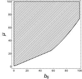
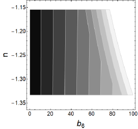
Figure 1: Left panel: The allowed values of $\mu$ and $b_{6}$ parameters (shaded region) for $B_{0}=0.1$, $n=-1.20$, $r_{0}=1$ and $a_{0}=-1$. Right panel: The allowed values of $n$ and $b_{6}$ parameters for different values $\mu$ parameter.

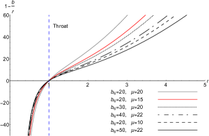
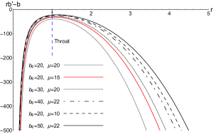
Figure 2: Left panel: Behavior of inverse of radial metric component for $n=-1.2$ and different values of $(b_{6},\mu)$ parameters. The blue dashed line indicates the location of the throat. Right panel: Plot of flare-out condition for $n=-1.2$ and different values of the parameters $b_{6}$ and $\mu$. We have set $B_{0}=0.1$, $r_{0}=1$ and $a_{0}=-1$.

The Left panel of Fig. (2) presents the inverse of radial metric component (${\sf g}_{rr}^{-1}$), where we observe that ${\sf g}_{rr}^{-1}$ is positive for $r>r_{0}$ and thus the metric signature is preserved in this range. To be a wormhole solution, one needs to impose that the throat flares out. This can be seen at the right panel of Fig. (2) as the satisfaction of flare-out condition. The left panel in Fig. (3) shows that the energy density and quantities $\rho+p_{r}$ and $\rho+p_{t}$ remain positive for the allowed values of Fig. (1); thus the WEC and NEC are satisfied throughout the spacetime. Following the results of [17], one may define a measure of exoticity of matter through the exoticity parameter $\xi$, given as [17],[15]

$$\xi(r)=\frac{\tau(r)-\rho(r)}{\mid\!\!\rho(r)\!\!\mid}=-\frac{\rho(r)+p_{r}(r)}{\mid\!\!\rho(r)\!\!\mid},$$ (53)

where, $\tau(r)=-p_{r}(r)$ is the radial tension. The positiveness of $\xi(r)$ signals exotic behavior of the matter. The right panel in Fig. (3) shows the behavior of exoticity parameter for allowed values of model parameters. It is seen that this parameter is negative at the throat and stays negative for $r>r_{0}$. Thus, there is no need of introducing exotic matter in order to construct the present wormhole solutions.

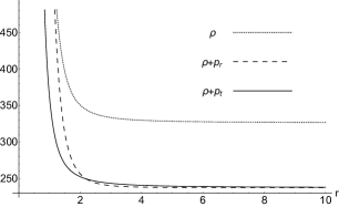
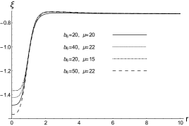
Figure 3: Left panel: Plot of WEC for $n=-1.2$ and $b_{6}=\mu=20$. Right panel: Plot of exoticity parameter against radial coordinate for $n=-1.2$ and different values of $(b_{6},\mu)$ parameters. We have set $B_{0}=0.1$, $r_{0}=1$, $a_{0}=-1$.

The wormhole configurations we have presented so far respect WEC and NEC with a non-exotic fluid as the supporting matter. In order to get a better understanding of the behavior of such a type of matter we proceed with considering a linear relation between pressure profiles and energy density with $r$-dependent state parameters as

$$p_{r}(r)=w_{r}(r)\rho(r),\leavevmode\nobreak\ \leavevmode\nobreak\ \leavevmode\nobreak\ \leavevmode\nobreak\ \leavevmode\nobreak\ \leavevmode\nobreak\ p_{t}(r)=w_{t}(r)\rho(r).$$ (54)

The state parameters will take the following form at the throat

$$w_{r0}=w_{r}(r_{0}) = \frac{3(3n+4)\left[2{a_{0}}{b_{6}}+\mu\left(2{b_{6}}+3\mu r_{0}^{2}\right)\right]}{8B_{0}^{2}{b_{6}}({a_{0}}+\mu)r_{0}^{2n+2}-9\left[2{a_{0}}\left({b_{6}}n-4\mu r_{0}^{2}\right)+\mu\left(2{b_{6}}n+\mu(3n-4)r_{0}^{2}\right)\right]},$$ (55)

$$w_{t0}=w_{t}(r_{0}) = \frac{-4B_{0}^{2}{b_{6}}({a_{0}}+\mu)r_{0}^{2n+2}-3\left[4{a_{0}}\left({b_{6}}+3\mu r_{0}^{2}\right)+\mu\left(4b_{6}-9\mu nr_{0}^{2}\right)\right]}{8B_{0}^{2}b_{6}(a_{0}+\mu)r_{0}^{2n+2}+9\left(-2a_{0}b_{6}n+8a_{0}\mu r_{0}^{2}-2b_{6}\mu n+\mu^{2}(4-3n)r_{0}^{2}\right)}.$$ (56)

At first glance, depending on the model parameters, the radial and tangential state parameters at wormhole throat can assume different values. However, these values have to fulfill the conditions on physical validity of the wormhole solution, i.e., conditions (i)-(iii). To this aim, we proceed with finding the allowed values for the pair $(b_{6},\mu)$ for different values of $n$ parameter (see the left panel in Fig. (1)). Then, we are able to evaluate the values of state parameters at the throat subject to the conditions stated above. By doing so, we obtain the bounds on state parameters at the throat as shown in the left panel of Fig. (4). We therefore observe that the state parameters obey the ranges $0.022\lessapprox w_{r0}\lessapprox 0.07$ and $-0.5\lessapprox w_{t0}\lessapprox-0.46$, respectively, hence the wormhole supporting matter respects the WEC and NEC at the throat. The right panel shows the behavior of state parameters versus radial coordinate where, we observe that the wormhole spacetime tends to an isotropic configuration in the limit $r\rightarrow\infty$. This behavior can be also verified through the anisotropy parameter, defined as, $\Delta(r)=p_{t}(r)-p_{r}(r)=\left[w_{t}(r)-w_{r}(r)\right]\rho(r)$. Since $\rho(r)>0$ throughout the spacetime, it is the sign of the term in square brackets that decides the geometry of wormhole configuration. Let us define the coordinate radius $r_{2}$ so that for $r_{0}<r_{2}<\infty$ we have $\Delta(r_{2})=0$, see the left panel of Fig. (5). We therefore note that since the ratio $2\Delta/r$ represents the force due to anisotropic nature of the configuration, we have an attractive geometry for $r_{0}<r<r_{2}$ and a repulsive geometry for $r_{2}<r<\infty$. The value of coordinate radius $r_{2}$ depends on model parameters, specifically for the present case, the smaller the absolute value of $n$ parameter, the larger the value of coordinate radius $r_{2}$. Moreover, having passed the negative values ($r>r_{2}$), the anisotropy parameter reaches a maximum value at $r=r_{3}$ where $\Delta^{\prime}(r_{3})=0$. As the left panel shows, the larger the absolute value of $n$ parameter, the closer the maximum value of anisotropy to the throat. One then may intuitively imagine that the rate of growth of spacetime torsion around the throat could affect the anisotropy of the wormhole configuration. As $r\rightarrow\infty$ we have $\Delta(r)\rightarrow 0$, thus asymptotically, the supporting matter of the wormhole configuration tends to an isotropic fluid.

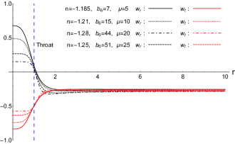
Figure 4: Left panel: The allowed values of state parameters at the wormhole throat for different values of $n$ parameter. Right panel: The behavior of state parameters $w_{r}(r)$ (black curves) and $w_{t}(r)$ (red curves) for different values of model parameters. The blue dashed line indicates the location of the throat. We have set $B_{0}=0.1$, $r_{0}=1$ and $a_{0}=-1$.

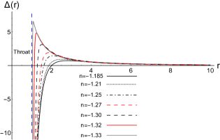
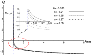
Figure 5: Left panel: The behavior of anisotropy parameter against the radial coordinate for different values of parameter $n$. Right panel: Deflection angle against closest distance approach for different values of $n$ parameter. We have set $B_{0}=0.1$, $b_{6}=10$, $\mu=5$, $r_{0}=1$ and $a_{0}=-1$. The blue dashed line indicates the location of the throat.

4 Gravitational Lensing Effects

One of the interesting ways for detecting wormholes is to search for their gravitational lensing effects. In the present section we investigate lensing features of the obtained wormhole solutions. To this aim we need to study the behavior of null geodesics traveling within the wormhole spacetime. The starting point of our study is the following Lagrangian describing the motion of photons in equatorial plane $\theta=\pi/2$,

$$2{\mathfrak{L}}=g_{\mu\nu}\dot{x}^{\mu}\dot{x}^{\nu}=-\dot{t}^{2}+\left(1-\frac{b(r)}{r}\right)^{-1}\dot{r}^{2}+r^{2}\dot{\phi}^{2},$$ (57)

where use has been made of the spacetime metric (25) and an overdot denotes derivative with respect to the curve parameter $\eta$. Because of spherical symmetry, the same results can be applied to all values of $\theta$. The Lagrangian ${\mathfrak{L}}(\dot{x},x)$ is constant along a geodesic curve, so one can classify the spacetime geodesics as, timelike geodesics (the world lines of freely falling particles) for which ${\mathfrak{L}}<0$, lightlike ones for which ${\mathfrak{L}}=0$ and spacelike geodesics for which ${\mathfrak{L}}>0$. Then, equation of photon trajectory takes the following form

$$\dot{r}^{2}+\left(1-\frac{b(r)}{r}\right)\left(\frac{h^{2}}{r^{2}}-{\mathcal{E}}^{2}\right)=0,$$ (58)

where ${\mathcal{E}}=\dot{t}$ is the total energy of the particle moving on its orbit and $h=r^{2}\dot{\phi}$ is its specific angular momentum. Consider now a light ray incoming from infinity, reaching the minimum distance $r_{\rm min}$ from the center of the gravitating body, emerging then in another direction. The deflection angle of the light ray as a function of the closet distance approach is given by [71]

$$\Theta(r_{\rm min})=-\pi+2\int_{r_{\rm min}}^{\infty}\frac{\mu dr}{\left[\left(r^{2}-rb(r)\right)\left(r^{2}-J^{2}\right)\right]^{\frac{1}{2}}},$$ (59)

where $J=h/{\mathcal{E}}$ is the impact parameter and $dr/d\phi=0$ at $r=r_{\rm min}$, so we have $J=r_{\rm min}$. Substituting solution (36) into the above expression, we obtain the deflection angle as

$$\Theta(r_{\rm min})=-\pi+2r_{\rm min}\int_{r_{\rm min}}^{\infty}\left(r^{2}-r_{\rm min}^{2}\right)^{-\frac{1}{2}}\left[r^{2}-\alpha_{1}r^{2}-\alpha_{2}r^{4}-\alpha_{3}r^{2(n+2)}-\alpha_{4}r^{\frac{4-3n^{2}}{3n+4}}\right]^{-\frac{1}{2}}dr.$$ (60)

In the right panel of Fig. (5) we have plotted the deflection angle as a function closest distance approach using numerical methods. It is therefore seen that the more the closest distance decreases, the more the deflection angle grows. Decreasing $r_{\rm min}$ further causes the light ray to infinitesimally come closer to the photon orbit making it to wind up for a large number of times before emerging out. The deflection angle will diverge, eventually, at a critical value of closet distance approach, $r_{\rm min}^{\rm cr}$ where light ray will loop around a circular photon orbit indefinitely. The set of these orbits constructs the photon sphere satisfying $\dot{r}=\ddot{r}=0$ [72] [73]. In [74], it has been shown that the wormhole throat can act as an effective photon sphere located at $r_{\rm min}^{\rm cr}=r_{0}$. Hence, as $r_{\rm min}\rightarrow r_{0}$, the deflection angle increases and diverges at the wormhole throat where an unstable photon sphere is present. As a result, the wormhole can produce infinite number of relativistic images of an appropriately placed light source. This infinite sequence corresponds to infinitely many light rays whose limit curve asymptotically spirals towards the unstable photon sphere [72]. Since the photon sphere coincides with the wormhole throat, such a sphere can be detected utilizing thoroughly and carefully designed modern instruments [73],[75], providing thus, possible observational proofs for the existence of the wormhole. The deflection angle decreases as $r_{{\rm min}}$ increases beyond $r_{0}$ (the light bears lesser bending) until the closest distance approach reaches a critical value at which $\Theta(r_{{\rm min}}^{\star})=0$, i.e., no deflection of light occurs, see the inset of Fig. (5). In such a situation, any incoming light ray from infinity that reaches the coordinate distance $r=r_{{\rm min}}^{\star}$, is scattered back to infinity without any spinning around the wormhole lens. Therefore the light ray does not undergo any net deflection by the gravitating object. For $r_{{\rm min}}>r_{{\rm min}}^{\star}$ the deflection angle is found to be negative, which can be interpreted as there is a repulsion of light by the wormhole configuration. A negative value for deflection angle has also been reported in gravitational lensing by a naked singularity [76]. It is noteworthy that, beside the lensing effects that can play a major role in detecting wormhole configurations, various observational aspects have been investigated so far with the aim of probing wormholes that might be living in our Universe. Among these studies we can quote: the study of particle trajectory in the wormhole spacetime [77], accretion disks around wormholes [78] and their gravitational wave signatures [79]. Another interesting candidate for extracting physical information from the wormhole spacetime is the shadow cast by it or its apparent shape [80]. As the shape of the shadow is merely determined by the background metric, the observation of such a phenomenon can provide useful information on the nature of the compact object and under some conditions, this interesting event can provide observational testbed for distinguishing the wormhole from other compact bodies. This idea has motivated many researchers to investigate observational aspects of wormholes, e.g., shadows cast by rotating [81] and charged wormholes [82] has been studied and in [83], the authors have developed the shadow-like images of wormholes surrounded by optically thin dust. The existence of unstable photon orbits is of crucial importance in studying wormhole shadows as these orbits define the boundary between capture and non-capture of the light rays around a wormhole configuration. Thus, the boundary of the shadow is only determined by the metric of spacetime since it corresponds to the apparent shape of the photon sphere as seen by a distant observer [81, 84] (see also [85] for more details). As the lensing effects and shadows are of significant importance for detecting astrophysical compact objects, especially wormholes, it is about time to probe the existence of such objects utilizing advanced instruments, e.g., the US-led Event Horizon Telescope (EHT) project and the European Black Hole Cam (BHC) project.

5 Concluding Remarks

In the present work, we tried to build and study static spherically symmetric wormhole configurations in a subclass of PGT Lagrangians that allow for spin-$0^{+}$ propagating modes. We therefore considered the field equations of PGT in the absence of spin of matter and followed the strategy of solving the field equations performed in [17]. It was found that in addition to GR terms, new geometric terms that come from spacetime torsion contribute to the EMT components. We then proceeded to find exact spacetimes that admit suitable wormhole configurations, considering the field equation derived from variation of gravitational Lagrangian with respect to the connection i.e., Eq. (21). The exact solution for a constant redshift shows that the wormhole’s shape has functional dependence on the torsion component $B(r)$. Assuming then a power-law behavior for torsion component, $B(r)=B_{0}r^{n}$, we provided the allowed regions for three of the model parameters ($n$, $b_{6}$ and $\mu$) for which the conditions on physical reasonability of the model are respected. We further realized that, for the obtained solutions, the supporting matter for wormhole geometry obeys the WEC and NEC. In order to study the nature of this type of matter, we assumed that its radial and tangential pressure profiles depend linearly on energy density with $r$-dependent state parameters, see Eq. (54). The behavior of these parameters was investigated and it was found that the matter threading the wormhole configuration can assume different equations of state (at the throat) depending on the model parameters, see Fig. (4). Furthermore, we provided the allowed values of state parameters at the throat subject to fulfillment of conditions on physical validity of the solutions. The anisotropy parameter for wormhole geometry was studied and it was observed that this parameter could admit different maxima near the throat depending on the growth rate of spacetime torsion. Finally we investigated gravitational lensing effects on the wormhole’s surrounding environment and it was found that the deflection angle of the incoming beam of light admits positive, zero and negative values. The situation of vanishing deflection angle occurs at different coordinate radii and the value of each radius depends on the behavior of spacetime torsion near the wormhole throat. We therefore observed that, depending on model parameters, the wormhole configuration can act as a converging or diverging lens. It is worth mentioning that, solutions comprising rich information on wormhole configurations in PGT may be found by taking, $i)$ a general form of the red-shift function, $ii)$ a non-zero spin density of matter distribution, and $iii)$ different functionalities of the torsion components. Specially the second case could provide a setting based on which the effects of spin on the geometry of a wormhole configuration can be surveyed. More interestingly, these effects can be helpful in probing the geometrical feature of the spacetime that couples to spin of matter, i.e., the spacetime torsion, via highly sensitive observational instruments. However, regarding these cases, the resultant field equations are too complicated to be solved analytically and more advanced mathematical techniques are needed in order to overcome the problem. Work along this line is currently in progress and the results will be reported as an independent work.

References

- [1] L. Flamm, Physik Z. 17, 448 (1916).
-
[2]
A. Einstein and N. Rosen, Phys. Rev. 48, 73 (1935);
D. R. Brill and R. W. Lindquist, Phys. Rev. 131, 471 (1963). -
[3]
C. W. Misner and J. A. Wheeler, Ann. Phys. 2, 525 (1957);
C. W. Misner, Phys. Rev. 118, 1110 (1960). -
[4]
J. A. Wheeler, Ann. Phys. 2, 604 (1957);
J. A. Wheeler, Geometrodynamics (Academic, New York, 1962). - [5] J. A. Wheeler, Phys. Rev. 97, 511 (1955).
- [6] S. W. Hawking, Phys. Rev. D 37, 904 (1988).
- [7] R. W. Fuller and J. A. Wheeler, Phys. Rev. 128, 919 (1962).
- [8] R. P. Geroch, J. Math. Phys. 8, 782 (1967).
- [9] K. Bronnikov, Acta Phys. Pol. B 4, 251 (1973).
- [10] H. G. Ellis, J. Math. Phys. 14, 104 (1973).
- [11] H. G. Ellis, Gen. Rel. Grav. 10, 105 (1979).
- [12] G. Clèment, Gen. Rel. Grav. 16, 131 (1984); Gen. Rel. Grav. 16, 477 (1984).
- [13] G. Clèment, Gen. Rel. Grav. 13, 747 (1981).
- [14] G. Clèment, Gen. Rel. Grav. 13, 763 (1981).
- [15] F. S. N. Lobo (Editor), “ Wormholes, Warp Drives and Energy Conditions,” Springer (2017).
- [16] K. A. Bronnikov, S. G. Rubin, “Black Holes, Cosmology and Extra Dimensions,” World Scientific (2013).
- [17] M. S. Morris and K. S. Thorne, Am. J. Phys. 56, 395 (1988).
- [18] M. S. Morris, K. S. Thorne and U. Yurtsever, Phys. Rev. Lett. 61, 1446 (1988).
-
[19]
M. Visser, Lorentzian Wormholes: From Einstein to Hawking (AIP, Woodbury, USA, 1995);
D. Hochberg and M. Visser, Phys. Rev. D 56, 4745 (1997). - [20] H. Epstein, V. Glaser and A. Jaffe, IL Nuovo Cimento, 36, 1016 (1965).
- [21] D. Hochberg, T. W. Kephart, Phys. Lett. B 268, 377 (1991).
- [22] G. Klinkhammer, Phys. Rev. D 43, 2542 (1991).
-
[23]
S. W. Hawking, Phys. Rev D 46, 603 (1992);
E. Poisson and M. Visser, Phys. Rev. D 52, 7318 (1995);
M. Chianese, E. Di Grezia, M. Manfredonia and G. Miele, Eur. Phys. J. Plus 132, 164 (2017). -
[24]
F. S. N. Lobo, Phys. Rev. D 71, 124022 (2005);
P. K. F. Kuhfittig, Class. Quant. Grav. 23, 5853 (2006);
F. S. N. Lobo, F. Parsaei and N. Riazi, Phys. Rev. D 87, 084030 (2013);
Y. Heydarzade, N. Riazi and H. Moradpour, Can. J. Phys. 93, 1523 (2015). - [25] V. Folomeev and V. Dzhunushaliev, Phys. Rev. D 89, 064002 (2014).
- [26] F. S. N. Lobo, Classical and Quantum Gravity Research, 1-78, (2008), Nova Sci. Pub. ISBN 978-1-60456-366-5, arXiv:0710.4474 [gr-qc].
- [27] F. Rahaman, P. Salucci, P. K. F. Kuhfittig, S. Ray and M. Rahaman, Ann. Phys., 350, 561 (2014).
-
[28]
S. Capozziello and M. De Laurentis, Phys. Rep., 509, 167 (2011);
A. De Felice and S. Tsujikawa, Living Rev. Rel., 13, 3 (2010);
C. Corda, Int. J. Mod. Phys. D 18, 2275 (2009). - [29] F. T.-Ortiz, S. K. Maurya, Pedro Bargueño, EPJC, 81, (2021) 426.
-
[30]
G. Dotti, J. Oliva, R. Troncoso, Phys. Rev. D 75, 024002 (2007);
H. Maeda, M. Nozawa, Phys. Rev. D 78, 024005 (2008);
M. H. Dehghani and Z. Dayyani, Phys. Rev. D 79, 064010 (2009);
M. R. Mehdizadeh and F. S. N. Lobo, Phys. Rev. D 93, 124014 (2016). - [31] H. Moradpour, N. Sadeghnezhad and S. H. Hendi, Can. J. Phys. 95, 1257 (2017).
-
[32]
N. M. Garcia and F. S. N. Lobo, Phys. Rev. D 82, 104018 (2010);
M. Zubair, S. Waheed and Y. Ahmad, Eur. Phys. J. C 76, 444 (2016). -
[33]
A. G. Agnese and M. La Camera, Phys. Rev. D 51, 2011 (1995);
K. K. Nandi, A. Islam, and J. Evans, Phys. Rev. D 55, 2497 (1997);
L. A. Anchordoqui, S. P. Bergliaffa, and D. F. Torres, Phys. Rev. D 55, 5226 (1997);
R. Shaikh and S. Kar, Phys. Rev. D 94, 024011 (2016). -
[34]
N. Furey and A. DeBenedictis, Class. Quantum Grav. 22, 313 (2005);
F. S. N. Lobo and M. A. Oliveira, Phys. Rev. D 80, 104012 (2009);
A. De Benedictis, D. Horvat, Gen. Relat. Gravit. 44, 2711 (2012);
M. Sharif and I. Nawazish, Annals of Physics, 389, 283 (2018). -
[35]
K. A. Bronnikov and A. M. Galiakhmetov, Grav. Cosmol. 21, 283 (2015);
Phys. Rev. D 94, 124006 (2016). -
[36]
M. R. Mehdizadeh and A. H. Ziaie, Phys. Rev. D 95, 064049 (2017);
Phys. Rev. D 99, 064033 (2019). -
[37]
S. H. Mazharimousavi, M. Halilsoy, and Z. Amirabi, Phys.
Rev. D 81, 104002 (2010);
P. Kanti, B. Kleihaus and J. Kunz, Phys. Rev. D 85, 044007 (2012);
G. Antoniou, A. Bakopoulos, P. Kanti, B. Kleihaus and Jutta Kunz, arXiv:1904.13091 [hep-th]. -
[38]
R. Shaikh, Phys. Rev. D 92, 024015 (2015);
F. Rahaman, N. Paul, A. Banerjee, S. S. De, S. Ray and A. A. Usmani, Eur. Phys. J. C 76, 246 (2016);
P. H. R. S. Moraes, P. K. Sahoo, Phys. Rev. D 96, 044038 (2017);
M. G. Richarte, I. G. Salako, J. P. Morais Graca, H. Moradpour, and A. ovgun, Phys. Rev. D 96, 084022 (2017);
K. Jusufi, N. Sarkar, F. Rahaman, A. Banerjee and S. Hansraj, Eur. Phys. J. C 78 349 (2018). - [39] F. W. Hehl, P. Von der Heyde, and G. D. Kerlick and J. M. Nester, Rev. Mod. Phys. 48, 393 (1976).
- [40] V. De Sabbata and M. Gasperini, “Introduction to Gravitation,”, World Scientific, Singapore (1986).
- [41] T. W. B. Kibble, J. Math. Phys. 2, 212 (1961).
- [42] M. Blagojevic, arXiv:gr-qc/0302040.
- [43] Y. N. Obukhov, Int. J. Geom. Meth. Mod. Phys. 3, 95 (2006).
- [44] Y. N. Obukhov, V. N. Ponomariev, and V. V. Zhytnikov, Gen. Rel. Grav. 21, 1107 (1989).
- [45] F. W. Hehl, J. D. McCrea, E. W. Mielke, and Y. Ne’eman, Phys. Rep. 258, 1 (1995).
- [46] M. Blagojevic, “Gravitation and Gauge Symmetries,” Institute of Physics, Bristol (2002).
- [47] M. Blagojevic and F. W. Hehl, “Gauge Theories of Gravitation: A reader with commentaries,” Imperial College Press, London, (2013).
-
[48]
A. V. Minkevich, Grav. Cosmol. 12, 11 (2006);
A. V. Minkevich and A. S. Garkun, Class. Quantum Grav. 23, 4237 (2006);
A. V. Minkevich, Acta Phys. Pol. B 38, 61 (2007);
A. V. Minkevich, A. S. Garkun and V. I. Kudin, Class. Quantum Grav. 24, 5835 (2007);
A. V. Minkevich, Ann. Fond. Louis de Broglie 32, 253 (2007);
H. Zhang and L. Xu, JCAP, 2019, 09 (2019);
H. Zhang and L. Xu, arXiv:1906.04340;
S. Akhshabi, E. Qorani, F. Khajenabi, EPL, 119, 29002 (2017). - [49] C. H. LEE, Phys. Lett. B, 130, 257 (1983).
- [50] J. A. R. Cembranosa, and J. G. Valcarcel, JCAP 01 (2017) 014.
- [51] S. S. Zamani, S. Akhshabi, Mod. Phys. Lett. A 36, 2150226 (2021).
- [52] J. M. Nester, in “Introduction to Kaluza-Klein Theories,” edited by H. C. Lee, World Scientific, Singapore (1984).
- [53] F. W. Hehl, in “Proceedings of the 6th Course of the International School of Cosmology and Gravitation on Spin, Torsion, and Supergravity,” edited by P. G. Bergmann and V. de Sabatta, Plenum, New York, (1980).
- [54] K. Hayashi and T. Shirafuji, Prog. Theor. Phys., 64, 866 (1980); 64, 883 (1980); 64, 2222 (1980).
- [55] E. W. Mielke, “Geometrodynamics of Gauge Fields, Akademie-Verlag, Berlin (1987).
- [56] F. Gronwald and F. W. Hehl, in “Proceedings of the 14th Course of the School of Gravitation and Cosmology (Erice),” editedby P. G. Bergmann, V. de Sabatta and H. J. Treder, World Scientific, Singapore (1996).
- [57] F. W. Hehl, Y. Ne’eman, J. Nitsch and P. Von Der Heyde, Phys. Lett. B, 78, 102 (1987).
- [58] E. Sezgin and P. van Nieuwenhuizen, Phys. Rev. D 21, 3269 (1980).
-
[59]
M. Blagojevic and I. A. Nikolic, Phys. Rev. D 28, 2455 (1983);
I. A. Nikolic, Phys. Rev. D 28, 2508 (1984). - [60] H. J. Yo and J. M. Nester, Int. J. Mod. Phys. D 8, 459 (1999).
- [61] H. Chen, J. M. Nester, and H. J. Yo, Acta Phys. Pol. B 29, 961 (1998).
- [62] R. Hecht, J. M. Nester, and V. V. Zhytnikov, Phys. Lett. A 222, 37 (1996).
- [63] H. J. Yo and J. M. Nester, Int. J. Mod. Phys. D 8, 459 (1999).
- [64] H.-J. Yo, and J. M. Nester, Mod. Phys. Lett. A 22, 2057 (2007).
- [65] K. F. Shie, J. M. Nester, and H. J. Yo, Phys. Rev. D 78, 023522 (2008).
- [66] H. Chen, F.-H. Ho, J. M. Nester, C.-H. Wang and H.-J. Yo, JCAP 0910:027 (2009).
- [67] P. Baekler, F. W. Hehl and J. M. Nester, Phys. Rev. D 83, 024001 (2011).
- [68] F. W. Hehl, “Gauge Theory of Gravity and Spacetime," arXiv:1204.3672 [gr-qc].
- [69] K. Hayashi and T. Shirafuji, Prog. Theor. Phys., 64, 1435 (1980).
-
[70]
S. M. Carroll, M. Hoffman, and M. Trodden, Phys. Rev. D 68, 023509 (2003);
Z.-K Guo, Y.-S. Piao and Y.-Z. Zhang, Phys. lett. B 594, 247 (2004); E. Elizalde, S. Nojiri, and S. D. Odintsov, Phys. Rev. D 70 043539 (2004); J.-gang Hao and X.-zhou Li, Phys. Rev. D 70 043529 (2004);
V. Faraoni, Class. Quant. Grav., 22, 3235 (2066);
H. Moradpour, R. C. Nunes, E. M. C. Abreu and J. A. Neto, Mod. Phys. Lett. A 32, 1750078 (2017);
H. Moradpour, S. A. Moosavi, I. P. Lobo, J. P. Morais Graca, A. Jawad and I. G. Salako, Eur. Phys. J. C, 78, 829 (2018). - [71] S. Weinberg, “Gravitation and cosmology: principles and applications of the general theory of relativity,” Wiley (1972).
- [72] W. Hasse and V. Perlick, Gen. Relativ. Gravit. 34, 415 (2002).
- [73] V. Perlick, Living Rev. Relativity, 7, 9 (2004).
- [74] R. Shaikh, P. Banerjee, S. Paul and T. Sarkar, Phys. Lett. B 789, 270 (2019).
-
[75]
M. Silvia and R. Esteban, "Gravitational Lensing And Microlensing," World Scientific (2002);
F. Courbin and D. Minniti, (Eds.), "Gravitational Lensing: An Astrophysical Tool," Springer (2008);
M. Kilbinger, Rep. Prog. Phys. 78, 086901 (2015);
S. Dodelson, "Gravitational Lensing," Cambridge University Press (2017);
S. E. Gralla, D. E. Holz and Robert M. Wald, arXiv:1906.00873 [astro-ph.HE]. -
[76]
K. S. Virbhadra, D. Narasimha, and S. M. Chitre, Astron. Astrophys. 337, 1 (1998);
K. S. Virbhadra and G. F. R. Ellis, Phys. Rev. D 65, 103004 (2002). - [77] T. Muller, Phys. Rev. D 77, 044043 (2008).
-
[78]
T. Harko, Z. Kovacs, and F. Lobo, Phys. Rev. D 78, 084005 (2008);
C. Bambi, Phys. Rev. D 87, 084039 (2013). -
[79]
V. Cardoso, E. Franzin and P. Pani, Phys. Rev. Lett. 116, 171101 (2016);
V. Cardoso, S. Hopper, C. F. B. Macedo, C. Palenzuela, and P. Pani, Phys. Rev. D 94, 084031 (2016);
S. Aneesh, S. Bose, and S. Kar, Phys. Rev. D 97, 124004 (2018). - [80] C. Bambi, Phys. Rev. D 87, 107501 (2013).
-
[81]
P. G. Nedkova, V. K. Tinchev, and S. S. Yazadjiev, Phys. Rev. D 88, 124019 (2013);
A. Abdujabbarov, B. Juraev, B. Ahmedov and Z. Stuchlik, Astrophys. Space Sci. 361, 226 (2016);
R. Shaikh, Phys. Rev. D 98, 024044 (2018);
G. Gyulchev, P. Nedkova, V. Tinchev and S Yazadjiev, 78, 544 (2018);
R. Shaikh, Phys. Rev. D 98, 024044 (2018). - [82] M. Amir, A. Banerjee and S. D. Maharaj, Annals of Phys. 400, 198 (2019).
- [83] T. Ohgami and N. Sakai, Phys. Rev. D 91, 124020 (2015).
- [84] H. Falcke, F. Melia, and E. Agol, Astrophys. J. 528, L13 (2000).
-
[85]
A. Grenzebach, “ The Shadow of Black Holes: An Analytic Description,” Springer (2016);
P. V. P. Cunha and C. A. R. Herdeiro, Gen. Relativ. Gravit. 50, 42 (2018).