Few-Shot Abstract Visual Reasoning With Spectral Features

Abstract

We present an image preprocessing technique capable of improving the performance of few-shot classifiers on abstract visual reasoning tasks. Many visual reasoning tasks with abstract features are easy for humans to learn with few examples but very difficult for computer vision approaches with the same number of samples, despite the ability for deep learning models to learn abstract features. Same-different (SD) problems represent a type of visual reasoning task requiring knowledge of pattern repetition within individual images, and modern computer vision approaches have largely faltered on these classification problems, even when provided with vast amounts of training data. We propose a simple method for solving these problems based on the insight that removing peaks from the amplitude spectrum of an image is capable of emphasizing the unique parts of the image. When combined with several classifiers, our method performs well on the SD SVRT tasks with few-shot learning, improving upon the best comparable results on all tasks, with average absolute accuracy increases nearly 40% for some classifiers. In particular, we find that combining Relational Networks with this image preprocessing approach improves their performance from chance-level to over 90% accuracy on several SD tasks.

1 Introduction

The field of artificial intelligence has slowly enveloped human skills ranging from those requiring formal reasoning to those requiring flexibility and intuition (such as image recognition or natural language understanding). The recognition of highly abstract concepts given few examples is a ubiquitous human skill that has yet to see significant progress. In particular, flexible machine learning techniques have not yet been found which can solve a certain type of visual reasoning task known as same-different (SD) problems given only few examples [1, 2]. Solving these problems requires reasoning about the similarity between patterns located within the same image, something humans perform with ease. In this work we present a conceptually simple image transformation which can be combined with few-shot image classifiers to perform well at these tasks.

Figure 1: Representative examples from the SVRT task set. For SVRT #1, class 1 contains two identical figures, while images from class 2 contain two unique figures. For SVRT #5, class 1 contains two pairs of identical figures, while class 2 contains four unique figures. For SVRT #22, class 1 contains three identical aligned shapes, while in class 2, the shapes are not identical. For all three of these tasks, deep learning approaches have been unable to achieve good performance, even with large amounts of training data. In contrast, our approach is capable of achieving high accuracies with only 10 labelled samples.

There are many potential sources of abstract visual reasoning tasks one could study. These include Bongard problems (given 6 labelled images, try find the rule separating them) [3], Raven’s Progressive Matrices (given observed sequences of tiles, identify the missing tile) [4], the CLEVR dataset (answer questions based on a scene of multiple objects) [5], and SVRT problems (given N labelled images, classify unseen images) [6]. Although the SVRT lacks the variation of hand-drawn Bongard Problems (23 tasks vs. 200), it contains a variety of highly abstract tasks while being procedurally generated. Unlike Raven’s Progressive Matrices or CLEVR tasks which have seen significant progress [7, 8], SVRT tasks have seen only partial success. It is worth noting that while creating a program to automatically solve these types of problems may often be easy (the images in these tasks are simple, consisting of simple objects on a solid white background), the difficulty comes from finding an approach capable of learning to solve the problems with a minimal amount of expert knowledge or feature engineering.

The 23 SVRT tasks can be split into two groups, based on the type of patterns separating the two classes: spatial relation (SR) problems (ex. shapes in a line vs. not in a line) and SD problems (ex. two pairs of unique shapes vs. two pairs of identical shapes) [1]. Previous attempts at these tasks have shown that convolutional neural networks, a staple of image classification research, are capable of solving SR problems given enough training data (20K in [1] and 1 million in [2]), but the SD problems have proven to be more difficult. Perhaps unexpectedly, even relational networks [9], which perform well on other reasoning tasks such as CLEVR, have demonstrated great difficulty in learning to solve same-different problems, requiring millions of training samples to achieve above chance-level performance [2].

Our new approach is inspired by an interesting point of overlap between image processing and visual saliency, namely, Fourier transforms. In image processing, it is well-known that unwanted periodic noise in images can be removed by manually zeroing-out corresponding peaks in the amplitude spectrum of the Fourier transform with so-called ’notch’ filters. Instead of manually removing peaks, a functionally similar approach is to smooth peaks, which can be done automatically. In [10], the authors point out that a Gaussian filtering operation on amplitude spectra is an elegant way to compute visual saliency maps. This technique works because non-salient parts of an image are often those which are frequently occurring, leading to peaks in the amplitude spectrum. The effectiveness of this simple approach for producing saliency maps can be seen in the bottom row of Figure 2. In this work, we apply this insight to solve SD tasks. Duplicated figures in SVRT images that undergo this amplitude spectrum filtering process are partially removed, whereas unique figures are largely untouched. This provides easily usable information for convolutional neural-network-based approaches to learn to classify images from SD tasks.

We observe that using these filtered spectra in place of the raw images, we are able to improve the state-of-the-art at few-shot learning SVRT SD tasks by an average of nearly 30%. By working towards solving these abstract visual problems in a simple and interpretable way, we demonstrate how analogous problems in other areas of machine learning may be approached.

The main contributions of this work are thus:

• We describe a novel approach for solving same-different visual reasoning tasks which exploits insights from visual saliency (Section 3).

• We establish the performance of several popular algorithms for few-shot learning on SVRT tasks (Section 4).

• We experimentally demonstrate that our approach allows for achieving state-of-the-art performance on all of the SVRT same-different tasks with few-shot learning (Section 4.3).

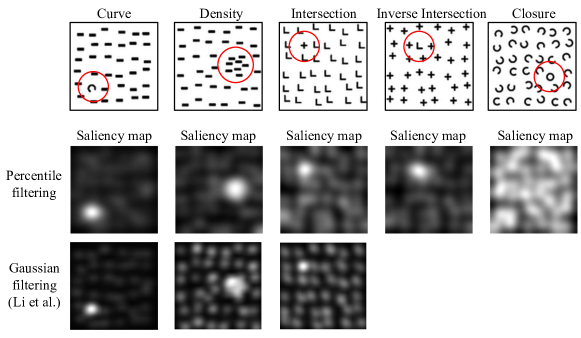
Figure 2: A comparison of saliency maps produced by percentile filtering and Gaussian filtering [10] on psychological test patterns from [11]. The expected salient locations are circled. As demonstrated by [11, 12, 13], the closure test proves to be difficult for many automated methods (this test was not reported by [10]). Following [11, 10], we square the raw saliency map to increase intensity contrast and apply a Gaussian filter to smooth the highlighted regions.

2 Related Work

In this section we first focus on previous work done on SD problems in particular, then provide an overview of relevant work on visual saliency maps.

2.1 Same-Different Visual Reasoning Tasks

With the aim of highlighting the difference in performance between humans and machines at solving visual reasoning tasks, François Fleuret et al. introduced the SVRT tasks in 2011 [6]. With their set of 23 binary classification tasks, the authors demonstrated that humans are much more proficient than a set of standard machine learning image classification techniques chosen at the time. In their few-shot experiments (only 10 training samples), the performance on most of the 23 tasks hovered around random. With 10,000 training images however, their best models were able to obtain 81% accuracy on SD tasks and 88% accuracy on SR tasks.

Studying the SVRT tasks with more modern computer vision approaches, Sebastian Stabinger et al. [1] trained LeNet [14] and GoogLeNet [15] CNNs on the tasks. They found that near-perfect performance was achievable on roughly half of the tasks, with the other half being significantly more difficult (near-random). By observing the abstract concepts required to solve each SVRT task, they noticed that this easy-difficult split closely corresponded to whether or not tasks required same-different comparisons, with a couple exceptions (they determined that a couple SD problems could be solved by exploiting simple pixel distribution patterns). The authors find that both CNN models perform very similarly, achieving perfect or near-perfect accuracies on the spatial-relation problems but poor performance on remaining tasks, despite training each network on 20,000 images. In [2], the authors use a minimal synthetic SVRT-like task for deeper exploration. They show that relational networks (RNs) [9] have trouble learning to solve these problems, requiring several million training samples before achieving above chance-level performance.

2.2 Saliency Maps

The aim of a visual saliency map is to indicate where a human is likely to gaze when looking at an scene, and these maps have proven to be useful for a wide variety of applications. Knowing where humans will attend in an image allows for such interesting applications as content aware image resizing [16, 17], segmentation of salient objects [18], aiding general objection-recognition [19], and video summarization [20].

Methods for calculating visual saliency can roughly be grouped by their underlying assumptions on the meaning of saliency. One common idea is that saliency is "an anomaly with respect to context" [21]. Separate approaches thus exist for various interpretations of "context". Approaches that use the local context around a pixel to determine saliency are often based on low-level visual features like colour, colour intensity, edge orientation, or texture [22]. Another set of approaches use a global context, where the saliency at a location depends on the entire image. One technique is to explicitly compare every patch in the image to a representative set of other patches. Those patches that are unique will have low cosine-similarities to other patches [12, 22].

Another group of approaches most relevant to the present paper has made use of operations on the Fourier transform of images. Adopting notation from [10], we consider $f(x,y)\xrightarrow{\mathcal{F}}\mathcal{F}(f)(u,v)$ to be the mapping of image $f(x,y)$ to the frequency domain, where $\mathcal{A}(u,v)=|\mathcal{F}(f)|$ is the amplitude spectrum and $\mathcal{P}(u,v)=angle(\mathcal{F}(f))$ is the phase spectrum. Xiaodi Hou and Liqing Zhang [11] proposed the idea that novelty in images is represented in the amplitude spectra of images as ’residuals’:

$$\mathcal{R}(u,v)=\mathcal{L}(u,v)-h_{n}\star\mathcal{L}(u,v),$$ (1)

where $\mathcal{L}(u,v)=\log{\mathcal{A}(u,v)}$ and $h_{n}$ is an $n\times n$ low-pass filter convolved over $\mathcal{L}(u,v)$. To produce the saliency map, $\mathcal{S}(x,y)$, the residual is then used in place of the original amplitude:

$$\mathcal{S}(x,y)=\mathcal{F}^{-1}[\mathcal{R}(u,v)\cdot exp(i\cdot\mathcal{P}(u,v))].$$ (2)

To achieve more visually pleasing results, they additionally square the elements of $\mathcal{S}(x,y)$ and smooth it with a low-pass filter. Soon after this work, [13] showed that similar results could be achieved by simply reconstructing the image using the phase spectrum:

$$\mathcal{S}(x,y)=\mathcal{F}^{-1}[1(u,v)\cdot exp(i\cdot\mathcal{P}(u,v))].$$ (3)

In [10], the authors suggest that these two approaches achieve very similar visual results because the residual of the amplitude spectrum is very similar to a plane (i.e. $1(u,v)$) and reconstructing images with only phase information functions similar to a gradient enhancement, highlighting object boundaries and textured parts of the image. This property leaves the methods ill-suited for identifying large salient regions or salient regions in front of noisy backgrounds.

Guided by the fact that repeated patterns (also called "non-salient" patterns) correspond to spikes in the amplitude spectrum, the authors of [10] reason that suppressing these peaks corresponds to leaving only the salient parts of an image. To perform this suppression so that sharper spikes are reduced more, a low-pass Gaussian filter, $g$, is used to obtain the smoothed amplitude spectrum:

$$\mathcal{A}_{\mathcal{S}}(u,v)=\mathcal{A}(u,v)\star g.$$ (4)

The saliency map can then be calculated with:

$$\mathcal{S}(x,y)=\mathcal{F}^{-1}[\mathcal{A}_{\mathcal{S}}(u,v)\cdot exp(i\cdot\mathcal{P}(u,v))].$$ (5)

This method is the most similar to our work described in the next section, One main difference is that we additionally consider a percentile filer. Additionally, instead of applying the inverse Fourier transform, we experimentally observe (Section 4.4) that training image classifiers directly on the filtered amplitude spectra leads to improved results on SD problems.

More recent CNN based approaches to saliency also exist [23, 24], however, work by [1, 2] suggests they do not transfer well to the abstract SVRT tasks despite the excellent performance of these approaches on calculating saliency maps.

3 Our Approach

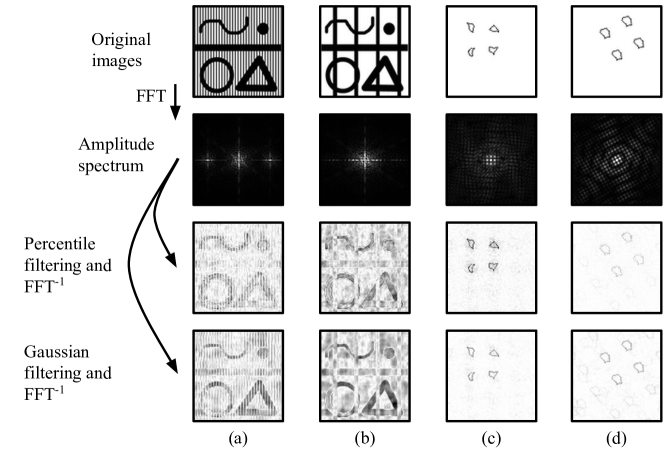
Figure 3: A demonstration of how non-unique parts of an image are affected by amplitude spectrum filtering. In the top row, columns (a) and (b) are images with varying scales of a repeated vertical lines and columns (c) and (c) are positive and negative samples from SVRT #15. The second row contains the amplitude spectra. The third and fourth rows contain the figures reconstructed with the percentile- and Gaussian-filtered amplitude spectra respectively. Note how the duplicated shapes are partially removed following filtering – for columns (c) and (d) containing SVRT samples, this effect is more clear with the percentile filter. The images in row 2 have undergone contrast enhancement for better printing quality. Rows 3 and 4 have been individually normalized so that their intensities lie in the range $[0,1]$.

The core of our SD problem-solving approach is based on the insight that peaks in the amplitude spectrum of an image correspond to the non-unique parts of that image, and removing these peaks corresponds to removing the non-unique parts of the image [10] (demonstrated in Figure 3). While deep convolutional neural networks have been able to solve a wide variety of visual tasks given only the raw images, they have thus far been unable to solve SD tasks this way [1, 2]. A motivation of our model is thus to find a simple transformation of the problem images such that when combined with CNN-based approaches, the classifiers are capable of extracting the necessary information to solve SD problems. Consider SVRT #1 from Figure 1 for example. If an image transformation were capable of making the non-unique figure outlines in class 1 lighter than the unique figure outlines in class 2, then a CNN classifier trained with gradient-descent would have no trouble identifying the relevant visual feature (namely, intensity). This is precisely what amplitude spectrum filtering allows us to do. The main way our primary approach differs from this is that instead of training the classifier on the inverse Fourier transform using the filtered amplitude, we provide the filtered amplitude spectrum directly to the classifier. In Section 4.4 we examine how using the filtered amplitude differs from using the inverse Fourier transform with the filtered amplitude.

In the remainder of this section, we first discuss the intuition of how amplitude filtering works to detect uniqueness and the difference between filtering methods we consider. Second, we discuss how these amplitude spectra fit into the rest of our problem-solving pipeline.

3.1 Amplitude Spectra Filtering

Removing non-uniqueness. Demonstrations of how amplitude filtering affects non-uniqueness in an image are provided in Figure 3. In columns (a) and (b), we can see an image with several unique figures and different scales of repeated (i.e. non-unique) vertical bars superimposed. In the amplitude spectra, these vertical bars correspond to the sharp peaks located symmetrically about the y-axis observable in the second row of the figure. By applying a filter to smooth or remove these peaks before reconstructing the image, we remove the cause of those peaks. As demonstrated, this works even when there are relatively few instances of the repeated shape (column (b)).

Filtering methods. To perform the amplitude spectrum filtering for our model, we consider Gaussian filtering (which was used in [10]) and (primarily) percentile filtering. Gaussian filtering of a matrix is performed by convolving a kernel whose values approximate a 2D Gaussian function:

$$G(x,y)=\frac{1}{2\pi\sigma^{2}}e^{-\frac{x^{2}+y^{2}}{2\sigma^{2}}},$$ (6)

where $x$ and $y$ are respectively the horizontal and vertical distances from the origin and $\sigma$ is the standard deviation. For each position, $\mathbf{u}$, in the amplitude spectrum of a discrete Fourier transform, the $p$-percentile filtered value is:

$$\mathcal{A}_{p}(\mathbf{u})=inf\left\{t\mid\frac{\#(\mathcal{A}(\mathcal{N}_{\mathbf{u}})\leq t)}{w^{2}}\geq p/100\%\right\},$$ (7)

where $\mathcal{N}_{\mathbf{u}}$ is a neighborhood of size $w\times w$ centered at $\mathbf{u}$ and $\#(\mathcal{A}(\mathcal{N}_{\mathbf{u}})\leq t)$ is the number of elements of $\mathcal{A}$ evaluated at each point of $\mathcal{N}_{\mathbf{u}}$ that are less than or equal to $t$. Where $\mathcal{N}_{\mathbf{u}}$ extends outside of $\mathcal{A}$, we consider $\mathcal{A}$ to evaluate to $0$. For convenience, in the rest of this paper we use $wf$ to be the $w$/(image width).

In Section 4.4 we demonstrate that both percentile and Gaussian filtering of amplitude spectra lead to state-of-the-art results on different SD tasks, with percentile filtering performing better on average.

3.2 Pipeline

Our primary approach for solving SD tasks follows a straightforward pipeline. First, for every training image for a task, we apply a percentile filter to the amplitude spectrum. Second, we train a classifier to predict class labels given the spectra (we discuss the classifiers used in Section 4.1). In Section 4.4 we will examine how the various choices in image transformation affect performance.

4 Experiments

4.1 Setup

To evaluate our image preprocessing approach for abstract visual reasoning, we make use of tasks from the SVRT challenge, consisting of 23 binary image classification tasks. As noted by [1], the SVRT tasks can be split into two groups: spatial relation (SR) problems and same-different (SD) problems. Solving SR problems requires attending to such feature as relative positioning, sizes, alignments, and grouping of figures. The SD problems require comparing individual figures within a single image to identify if they are identical, often under invariants such as scaling or rotation. In particular, we use the task type grouping proposed by [2], so that there are 9 SD tasks and 14 SR tasks.

We combine our image preprocessing technique with the following few-shot classifiers (with their abbreviated names). VGG-pt: pre-trained VGG16 [25] feature extractor with k-nearest neighbors classifier. MAML: model-agnostic meta-learning [26]. PN: Prototypical Networks [27]. RN: Relational Networks [9]. Network architectures, training details, and hyperparameters are described in the supplementary material. Fleuret refers to the Adaboost+spectral features model from [6], where the only other comparable results on few-shot learning of these tasks is available. The feature type abbreviations are as also follows (with more feature types examined in Section 4.4). Raw: original grayscale images. $\mathcal{A}$: unfiltered amplitude spectra. $\mathcal{A}_{p}$: percentile-filtered amplitude spectra.

4.2 Results At a Glance

Table 1 contains a high-level summary of how amplitude spectra filtering makes few-shot learning of SD tasks easier. In particular, we can make the following observations:

• By using $\mathcal{A}_{p}$ features for SD tasks, all classifiers tested go from performing at chance-level to above 70% accuracy with only 10 training samples.

• Relational Networks [9] and Prototypical Networks [27] improve the most with $\mathcal{A}_{p}$ features on SD tasks.

• When solving SR tasks, $\mathcal{A}_{p}$ features appear to make learning slightly easier, but $\mathcal{A}$ features perform better.

Table 1: The test results for each of the four classifiers we use are averages across all SD and SR problems separately and evaluated with the two baseline feature sets (the original image: raw and the unfiltered amplitude spectrum: $\mathcal{A}$).

Task type	Feature type	VGG-pt	MAML	PN	RN
	raw	50.7%	50.0%	50.7%	49.6%
SD	$\mathcal{A}$	60.5%	61.5%	63.4%	66.6%
	$\mathcal{A}_{p}$	70.1%	78.4%	78.7%	79.1%
	raw	56.5%	51.8%	49.3%	50.0%
SR	$\mathcal{A}$	58.5%	59.3%	62.9%	55.2%
	$\mathcal{A}_{p}$	53.4%	56.2%	55.9%	56.1%

Table 2: A comparison of existing results (Fleuret et al. [6]) to four CNN-based few-shot classifiers utilizing $\mathcal{A}_{p}$ features and 10 labelled samples. All four CNN classifiers outperform the existing results on every SD task. On several tasks, our approach is capable of achieving > 95% accuracy.

	SVRT SD Task
	1	5	7	15	16	19	20	21	22	Average
Fleuret	53.0%	47.0%	47.0%	54.0%	62.0%	51.0%	48.0%	39.0%	53.0%	50.4%
VGG-pt	89.2%	70.3%	52.2%	91.4%	98.8%	55.9%	51.9%	50.0%	70.7%	70.1%
MAML	99.8%	92.5%	58.4%	100.0%	96.3%	56.9%	56.0%	50.6%	95.3%	78.4%
PN	99.6%	95.9%	58.6%	99.6%	97.3%	56.1%	55.5%	49.6%	95.7%	78.7%
RN	99.9%	94.7%	60.8%	98.7%	98.1%	56.4%	55.3%	50.3%	97.6%	79.1%

Table 3: A comparison on the SR tasks of existing results and the three CNN-based approaches utilizing $\mathcal{A}$ features. MT, PN, and VGG-pt all perform quite close to each other, achieving approximately 8% better than Fleuret et al. on average.

	SVRT SR Task
	2	3	4	6	8	9	10	11	12	13	14	17	18	23	Average
Fleuret	55.0%	54.0%	56.0%	50.0%	57.0%	52.0%	50.0%	52.0%	46.0%	50.0%	51.0%	59.0%	50.0%	53.0%	52.5%
VGG-pt	66.2%	50.5%	66.6%	51.3%	75.0%	50.7%	71.2%	50.7%	57.2%	53.7%	67.6%	53.2%	50.8%	54.8%	58.5%
MAML	68.9%	56.1%	61.4%	50.3%	73.8%	51.2%	74.6%	60.1%	54.2%	65.1%	58.9%	51.9%	51.3%	52.0%	59.3%
PN	77.8%	58.2%	66.6%	50.8%	83.4%	51.4%	83.7%	64.1%	54.8%	70.4%	59.8%	53.3%	53.9%	52.0%	62.9%
RN	67.8%	51.2%	53.9%	51.1%	57.1%	51.1%	67.1%	52.8%	51.6%	62.1%	53.4%	51.6%	51.0%	50.4%	55.2%

4.3 A Closer Look

Same-different tasks. Perhaps the most immediate observation from Table 2 is the contrast in performance between classifiers utilizing $\mathcal{A}_{p}$ features and the existing results. On every task, our approaches outperform Fleuret et al., with the best classifier, Relational Networks, achieving an accuracy nearly 30% higher on average. Two problems where our models perform particularly well are #1 and #15. In class 1 for both tasks, some number of identical shapes are present (2 and 4 respectively), while in class 2, the shapes are all unique. These represent the most purely same-different problems. The highest performance of Fleuret et al. is achieved on #16 – in this task, both classes contain six identical shapes, but in class 1, the shapes on one side of the image can be obtained from those on the other side by reflection about the vertical image bisector. In class 2, the positions of the shapes are reflected, but not the details of the shapes themselves.

Spatial relation tasks. Table 3 contains the results using the best-performing feature type on these tasks, $\mathcal{A}$, according to Table 1. Aside from when using the RN classifier, this feature type performs similarly for both SD and SR problems, and consistently better than the raw images. This suggests that while $\mathcal{A}$ is not very useful for CNNs in providing uniqueness-type information, these features contain information difficult for CNNs to extract from raw images. On these tasks, the spectral features allow us to achieve up to 10% higher on average than Fleuret et al. with the PN classifier. Previous work has shown that using the raw images, CNNs can achieve very high accuracies on the SR tasks when given a large amount of training data [1, 2], but in this few-shot case we observe that the raw images only achieve up to 56.5% accuracy with the VGG-pt classifier, lower than the high-90s averages reported by [1] with 20,000 training samples and [2] with several million training samples. This demonstrates that improving few-shot performance on the SVRT SR tasks is worth further study.

4.4 Effects of Hyperparameters

Table 4: A comparison of the SD task performance of various feature types considered. $\mathcal{A}_{g}$ refers to the Gaussian-filtered amplitude spectra and $\mathcal{S}_{p}$ refers to the saliency map produced by taking the inverse Fourier transform with the original phase spectrum and the percentile-filtered amplitude.

	SVRT SD Task
	1	5	7	15	16	19	20	21	22	Average
raw	51.0%	49.5%	50.3%	52.5%	50.8%	50.3%	49.8%	50.8%	50.9%	50.7%
$\mathcal{A}$	63.3%	66.1%	54.2%	76.5%	58.9%	53.1%	51.6%	49.0%	71.7%	60.5%
$\mathcal{A}_{p}$	89.2%	70.3%	52.2%	91.4%	98.8%	55.9%	51.9%	50.0%	70.7%	70.1%
$\mathcal{A}_{g}$	64.6%	63.7%	58.3%	85.8%	67.2%	57.1%	53.5%	50.8%	77.5%	64.3%
$\mathcal{S}_{p}$	86.5%	62.4%	52.8%	88.4%	52.1%	52.1%	49.8%	50.4%	69.0%	62.6%

Choice of image transformation. In Table 4 we provide support for our choice of percentile-filtered amplitude spectra as the primary image preprocessing approach in our experiments. For these comparisons, we report the results of the VGG-pt classifier (chosen for its speed, as no neural networks require training). While both filtering methods (percentile and Gaussian) achieve the best performance on subsets of the SD tasks, percentile filtering achieves a 6% higher average accuracy than Gaussian filtering. Additionally, while it may be more intuitive to reconstruct the images with the filtered spectra before training the classifiers (feature type $\mathcal{S}_{p}$), Table 4 demonstrates that this achieves 8% lower than the $\mathcal{A}_{p}$, but still better than the raw images and the unfiltered amplitude spectra. However, we note that constructing saliency maps is often subject to additional post-processing parameters which we did not tune.

Filter parameters. We found that the most important parameter for the percentile filter was the size of the neighborhood around each point, $wf$, used to calculate the p-percentile, with larger values performing better. Unfortunately, calculating the p-percentile on a window requires first ranking every value, making the calculation slow for large windows. Thus, while we only tried $wf$ values up to 0.2, we strongly suspect that using larger values would improve performance on the SD tasks by several percent. For the $p$ value, we found 10 to generally perform best during hyperparameter tuning on the validation set, but with only minor performance decreases when 5 or 20 were used. When tuning the Gaussian kernel to produce the results in Table 4, we found the optimal value for $\sigma$ to sharply increase at 2, and slowly fall off for larger values.

5 Conclusion

We have presented an image preprocessing technique allowing few-shot deep learning classifiers to achieve improved accuracy on same-different (SD) problems. SD problems are a fundamental type of visual reasoning task often trivial for humans to solve with few samples while deep learning approaches training on millions of samples have been unsuccessful. Discovering machine learning approaches capable of solving these tasks is valuable in working towards automating highly abstract human skills.

To solve SD problems, we propose training CNN-based classifiers on the percentile-filtered amplitude spectra. As has been previously established with Gaussian filters, filtering these spectra correspond to removing the non-unique parts of an image. In line with previous work suggesting that fully convolutional approaches have difficulty learning to solve SD tasks, we demonstrate that a variety of state-of-the-art few-shot classifiers achieve only 50% binary classification accuracy on SD problems when trained on raw images. However, combining the classifiers with our image preprocessing technique allows them to achieve between 70% and 80% accuracy, outperforming the existing comparable state-of-the-art on SVRT SD tasks in the few-shot case, solidifying the effectiveness of this approach.

Appendix A Network architecture and hyperparameters

Here we discuss the implementation details and hyperparameters used for each model in our experiments. For all models, we use SVRT images of size 96x96, and for each SVRT task, we train models with 10 labelled samples (to compare to the few-shot experiments done in [6]) and evaluate on 1000 samples, where performance is measured with classification accuracy. To produce all experimental results, we average over 10 trials. For hyperparameter tuning, we average across 5 trials for each measurement on only the SD tasks, using 1000 validation images for each task. To produce the test results, we average across 10 trials, with 1000 different unseen test images each trial. For model training, we use 10 new images each trial. The code to generate samples for SVRT tasks is publicly available at http://www.idiap.ch/~fleuret/svrt/. Next, we discuss the details of tuning each classifier.

Transfer Learning. For this model, we used the VGG16 architecture pre-trained on ImageNet [25] and provided through Keras [28]. We extract features from the last set of convolutions. For the classifier, we use k-nearest neighbors. The value for $k$ was chosen from $\{1,3,5\}$ and the best value was found to be $k=1$ for all feature types.

Prototypical Networks. We use a publicly available implementation (https://github.com/orobix/Prototypical-Networks-for-Few-shot-Learning-PyTorch) with the same architecture for the embedding stage as in [27] and [29]. Three training samples are randomly chosen from each class for its support set. The optimal number of epochs was chosen from $\{8,16,32,64\}$ to maximize the average score on validation SD problems. When training on raw images, 32 epochs was found to perform best, and 64 epochs was found to perform best when using the spectral features.

MAML. We use a publicly available implementation (https://github.com/katerakelly/pytorch-maml) with the same architecture and hyperparameters as in the supervised Omniglot experiments in [26]. However, we choose the number of training epochs from ${8,16,32,64}$ to maximize the average score across validation SD problems. When training on raw images, 8 epochs was found to perform best, and 32 epochs was found to perform best when using the spectral features.

Relational Networks. We use a publicly available implementation (https://github.com/kimhc6028/relational-networks) with the same architecture used for CLVER in [9]. However, since this model is originally designed for tasks which contain images paired with textual questions, we modify the model by removing components associated with question processing so it can be applied to SVRT tasks. We select the number of training epochs from $\{64,128,256\}$ and learning rate from $\{1\text{e-}4,2.5\text{e-}4,1\text{e-}5\}$. When training on raw images, 128 epochs and learning rate of $1\text{e-}4$ was selected. When training on spectral features, 256 epochs and a learning rate of $5\text{e-}4$ were selected.

When optimizing the parameters for the percentile-filter for each classifier, we chose $p$ from $\{5,10,20,40\}$ and $wf$ from $\{0.05,0.1,0.2\}$. The optimal values for $p$ and $wf$ were identified to be 10 and 0.2 respectively for all classifiers, except for the transfer learning model, which used $p=10$ and $wf=0.2$.

References

- [1] Sebastian Stabinger, Antonio Rodríguez-Sánchez, and Justus Piater. 25 years of cnns: Can we compare to human abstraction capabilities? In International Conference on Artificial Neural Networks, pages 380–387. Springer, 2016.
- [2] Matthew Ricci, Junkyung Kim, and Thomas Serre. Not-so-clevr: Visual relations strain feedforward neural networks. arXiv preprint arXiv:1802.03390, 2018.
- [3] Mikhail M Bongard. The problem of recognition. Fizmatgiz, Moscow, 1967.
- [4] John C Raven et al. Raven’s progressive matrices. Western Psychological Services Los Angeles, CA, 1938.
- [5] Justin Johnson, Bharath Hariharan, Laurens van der Maaten, Li Fei-Fei, C Lawrence Zitnick, and Ross Girshick. Clevr: A diagnostic dataset for compositional language and elementary visual reasoning. In Proceedings of the IEEE Conference on Computer Vision and Pattern Recognition, pages 2901–2910, 2017.
- [6] François Fleuret, Ting Li, Charles Dubout, Emma K Wampler, Steven Yantis, and Donald Geman. Comparing machines and humans on a visual categorization test. Proceedings of the National Academy of Sciences, 2011.
- [7] Adam Santoro, Felix Hill, David Barrett, Ari Morcos, and Timothy Lillicrap. Measuring abstract reasoning in neural networks. In International Conference on Machine Learning, pages 4477–4486, 2018.
- [8] Drew A Hudson and Christopher D Manning. Compositional attention networks for machine reasoning. arXiv preprint arXiv:1803.03067, 2018.
- [9] Adam Santoro, David Raposo, David G Barrett, Mateusz Malinowski, Razvan Pascanu, Peter Battaglia, and Timothy Lillicrap. A simple neural network module for relational reasoning. In Advances in neural information processing systems, pages 4967–4976, 2017.
- [10] Jian Li, Martin D Levine, Xiangjing An, Xin Xu, and Hangen He. Visual saliency based on scale-space analysis in the frequency domain. IEEE transactions on pattern analysis and machine intelligence, 35(4):996–1010, 2013.
- [11] Xiaodi Hou and Liqing Zhang. Saliency detection: A spectral residual approach. In Computer Vision and Pattern Recognition, 2007. CVPR’07. IEEE Conference on, pages 1–8. IEEE, 2007.
- [12] Hae Jong Seo and Peyman Milanfar. Static and space-time visual saliency detection by self-resemblance. Journal of vision, 9(12):15–15, 2009.
- [13] Chenlei Guo, Qi Ma, and Liming Zhang. Spatio-temporal saliency detection using phase spectrum of quaternion fourier transform. In 2008 IEEE Conference on Computer Vision and Pattern Recognition, pages 1–8. IEEE, 2008.
- [14] Yann LeCun, Bernhard Boser, John S Denker, Donnie Henderson, Richard E Howard, Wayne Hubbard, and Lawrence D Jackel. Backpropagation applied to handwritten zip code recognition. Neural computation, 1(4):541–551, 1989.
- [15] Christian Szegedy, Wei Liu, Yangqing Jia, Pierre Sermanet, Scott Reed, Dragomir Anguelov, Dumitru Erhan, Vincent Vanhoucke, and Andrew Rabinovich. Going deeper with convolutions. In Proceedings of the IEEE conference on computer vision and pattern recognition, pages 1–9, 2015.
- [16] Bongwon Suh, Haibin Ling, Benjamin B Bederson, and David W Jacobs. Automatic thumbnail cropping and its effectiveness. In Proceedings of the 16th annual ACM symposium on User interface software and technology, pages 95–104. ACM, 2003.
- [17] Shai Avidan and Ariel Shamir. Seam carving for content-aware image resizing. In ACM Transactions on graphics (TOG), volume 26, page 10. ACM, 2007.
- [18] Esa Rahtu, Juho Kannala, Mikko Salo, and Janne Heikkilä. Segmenting salient objects from images and videos. In Computer Vision–ECCV 2010, pages 366–379. Springer, 2010.
- [19] Ueli Rutishauser, Dirk Walther, Christof Koch, and Pietro Perona. Is bottom-up attention useful for object recognition? In Computer Vision and Pattern Recognition, 2004. CVPR 2004. Proceedings of the 2004 IEEE Computer Society Conference on, volume 2, pages II–II. IEEE, 2004.
- [20] Yu-Fei Ma, Xian-Sheng Hua, Lie Lu, and Hong-Jiang Zhang. A generic framework of user attention model and its application in video summarization. IEEE transactions on multimedia, 7(5):907–919, 2005.
- [21] Meng Wang, Janusz Konrad, Prakash Ishwar, Kevin Jing, and Henry Rowley. Image saliency: From intrinsic to extrinsic context. In Computer Vision and Pattern Recognition (CVPR), 2011 IEEE Conference on, pages 417–424. IEEE, 2011.
- [22] Stas Goferman, Lihi Zelnik-Manor, and Ayellet Tal. Context-aware saliency detection. IEEE transactions on pattern analysis and machine intelligence, 34(10):1915–1926, 2012.
- [23] Matthias Kümmerer, Lucas Theis, and Matthias Bethge. Deep gaze i: Boosting saliency prediction with feature maps trained on imagenet. arXiv preprint arXiv:1411.1045, 2014.
- [24] Srinivas SS Kruthiventi, Kumar Ayush, and R Venkatesh Babu. Deepfix: A fully convolutional neural network for predicting human eye fixations. IEEE Transactions on Image Processing, 26(9):4446–4456, 2017.
- [25] Karen Simonyan and Andrew Zisserman. Very deep convolutional networks for large-scale image recognition. arXiv preprint arXiv:1409.1556, 2014.
- [26] Chelsea Finn, Pieter Abbeel, and Sergey Levine. Model-agnostic meta-learning for fast adaptation of deep networks. In Proceedings of the 34th International Conference on Machine Learning-Volume 70, pages 1126–1135. JMLR. org, 2017.
- [27] Jake Snell, Kevin Swersky, and Richard Zemel. Prototypical networks for few-shot learning. In Advances in Neural Information Processing Systems, pages 4077–4087, 2017.
- [28] François Chollet. keras. https://github.com/fchollet/keras, 2015.
- [29] Brenden Lake, Ruslan Salakhutdinov, Jason Gross, and Joshua Tenenbaum. One shot learning of simple visual concepts. In Proceedings of the Annual Meeting of the Cognitive Science Society, volume 33, 2011.