Graph Generation with Variational Recurrent Neural Network
Abstract
Generating graph structures is a challenging problem due to the diverse representations and complex dependencies among nodes. In this paper, we introduce Graph Variational Recurrent Neural Network (GraphVRNN), a probabilistic autoregressive model for graph generation. Through modeling the latent variables of graph data, GraphVRNN can capture the joint distributions of graph structures and the underlying node attributes. We conduct experiments on the proposed GraphVRNN in both graph structure learning and attribute generation tasks. The evaluation results show that the variational component allows our network to model complicated distributions, as well as generate plausible structures and node attributes.
1 Introduction
Leveraging the structural relationship over data points have been proven to be beneficial for problems in different research domains [5, 10, 13, 15, 18]. Despite the great success of graph neural networks in graph embedding and supervised settings, graph generation remains a challenging problem. To learn and generate graph structures, a generative graph model needs to capture the subtle relationships between node entities. Prior works have used variational Bayes model [8, 17], normalizing flow [2], or generative adversarial network [4] to learn the complex underlying distributions of such relationships, and achieve promising results [6, 9, 11, 12, 16]. However, these models are only applicable to small scale graphs due to their limited scalability. To cope with this issue, Graph Recurrent Neural Network (GraphRNN) [20] simplified the generation problem as a sequence prediction problem. GraphRNN cuts down the computational cost by mapping graphs into sequences such that the model only has to consider a subset of nodes during edge generation. While achieving successful results in learning graph structures, GraphRNN cannot faithfully capture the distribution of node attributes (Section 3).
In this paper, we propose a novel method for graph representation and generation to address the shortcomings explained above. Our contributions are summarized as follows: (1) A new formulation of an autoregressive variational autoencoder (VAE) [1, 3, 8, 14] for graph generation which yields a high-capacity model to capture latent factors over graphs with diverse modalities and complicated structural dependencies, while being as scalable as GraphRNN. (2) An algorithm to learn the joint probability distribution of the graph structure as well as the node attributes. (3) Experimental studies with successful results, competitive to the state-of-the-art models for graph generation.
2 The Proposed Method
In this section, we first introduce the problem and then describe our proposed GraphVRNN model. Please refer to Appendix A for the background on VAE and GraphRNN.
2.1 Problem Definition
Let be an undirected graph with nodes, where is the adjacency matrix and is the attribute matrix. Our goal is to model the joint probability distribution of the graph structure and the node attributes, i.e., .

2.2 Graph Recurrent Neural Network with Variational Bayes
In this section, we propose a VAE formulation to learn a model for , which can represent both graph structure and node attributes. Following the GraphRNN [20] approach to graph generation, we map a graph to sequences under Breadth-first Search (BFS) policies:
| (1) |
where is a sequence under a possible node permutation produced by BFS, and is the adjacency vector (or edge connections) between node and its previously generated nodes. Likewise, is the sequence of node attribute vectors under the same permutation . This sequential setting not only improves scalability but also alleviates the problem with node matching and non-unique representations during training [20]. Given this, the objective is reformulated to model :
| (2) |
where is the set of all possible permutations which gives . Using conditional VAE (CVAE) [17] formulation and defining the proposal distributions and prior distributions for each step in the sequence, the lower bound for the likelihood of under policy , i.e., is derived as
| (3) |
where is the Kullback–Leibler (KL) divergence and is a hyperparameter for tuning the KL penalty. An overview of the proposed Graph Variational Recurrent Neural Network (GraphVRNN) is illustrated in Figure 1. In this network, a node-level RNN is used to keep the history of and . The output is fed to a multi-layer perceptron (MLP) modeling the proposed posterior . At the bottom, the prior is modeled similarly but the input is one step behind. The proposal and prior distributions can be sampled to produce latent codes . Next, and the historical information (encoded by the node-level RNN) are concatenated and go through the decoding networks and to generate and then . We use an edge-level RNN as to decode step by step. As for the attribute decoder , we use an MLP. The model is trained by optimizing Eq. 3 using re-parameterization trick [8]. For implementation details, please refer to Appendix B.
| (max,max) | Ego-small (18, 69) | Com-small (20, 70) | Com-mix (40, 198) | ||||||
|---|---|---|---|---|---|---|---|---|---|
| D. | C. | O. | D. | C. | O. | D. | C. | O. | |
| GraphVAE [16] | 0.130 | 0.170 | 0.050 | 0.350 | 0.980 | 0.540 | - | - | - |
| DeepGMG [11] | 0.040 | 0.100 | 0.020 | 0.220 | 0.950 | 0.400 | - | - | - |
| GraphRNN | 0.076 | 0.298 | 0.008 | 0.020 | 0.061 | 0.009 | 0.045 | 0.045 | 0.046 |
| GraphVRNN-nlp | 0.026 | 0.144 | 0.008 | 0.009 | 0.040 | 0.005 | 0.043 | 0.051 | 0.047 |
| GraphVRNN | 0.052 | 0.184 | 0.010 | 0.015 | 0.057 | 0.005 | 0.038 | 0.047 | 0.039 |
3 Experiments
We conduct experiments to evaluate GraphVRNN’s ability to (1) model graph structures with complex latent distribution, (2) generate both plausible graph structures and attributes. To examine the effect of the prior network, we include a variant of GraphVRNN with simple prior (GraphVRNN-nlp). We adopt the maximum mean discrepancy (MMD) measurement proposed in [20] as the evaluation metric. For each dataset, we train all models for 5 runs, and report the averaged MMD of degree (D.), orbits (O.) and clustering coefficient (C.) between the generated examples and the testing set. A lower number implies a better result. For all the datasets considered in our experiments, we use of the graphs as training set, and the remaining as testing set.
3.1 Modeling Graph Structure
To evaluate the performance of GraphVRNN on learning graph structures, we first consider two small-scale datasets: (1) Ego-small: a 1-hop citation dataset with 200 graphs with nodes for each graph, and (2) Com-small: 500 2-community graphs with per graph ( nodes in each community). The probability that a pair of nodes is connected is if the nodes are in the same community, and otherwise.
We present the evaluation results in Table 1. GraphVRNN shows superior results than GraphRNN in all three MMD metrics. Interestingly, GraphVRNN-nlp exhibits better performance than the model with learned prior. This could be due to that the small-scale dataset does not have complex distribution that requires a strong prior for inference. Overall, the results indicate that the variational component in the proposed models help capture both the local and global structures of a small graph dataset.
To further test the efficacy of each model in handling larger graphs, we consider the Com-mix dataset. Similar to Com-small, Com-mix dataset consists of 500 2-community graphs but with . In addition, there are two types of graphs in this dataset: one with equal intra-connection probability for both communities, and the other with and for the two communities in the graphs (details in Appendix C). These settings challenge the scalability of the models, and test the models’ capability of learning the complex distribution of graph structures and types.
We show the results in Table 1. One can see that GraphVRNN shows superior performance on modeling the complicated intra-connection probability in Com-mix, which is reflected on the lower degree MMD. In addition, as the training/testing graphs get larger, GraphVRNN starts showing advantages over GraphVRNN-nlp. The results suggest that the learned prior network is helpful for modeling more intricate structures. Finally, we observed that GraphVRNN is insensitive to coeffient in the graph structure learning tasks.
3.2 Generating Attributes and Structures
| (max,max) | Com-attr (60,268) | Earth Mover’s Dist. | |||||
|---|---|---|---|---|---|---|---|
| D. | C. | O. | Com1 | Com2 | All | ||
| GraphRNN | 0.012 | 0.015 | 0.019 | 0.453 | 0.640 | 0.460 | |
| GraphVRNN-nlp | 0.017 | 0.015 | 0.018 | 0.302 | 0.400 | 0.290 | |
| GraphVRNN-0.5 | 0.016 | 0.021 | 0.024 | 0.178 | 0.095 | 0.113 | |
| GraphVRNN-1.0 | 0.014 | 0.015 | 0.022 | 0.382 | 0.265 | 0.267 | |
We have shown that GraphVRNN has comparable or even better ability to model the graph pattern than its non-variational counterpart. Finally, we test GraphVRNN’s ability to capture the latent spaces for generating graph structures and attributes simultaneously. Here, we consider Com-attr dataset, a variant of Com-small dataset with even larger graph ( nodes per graph). Moreover, nodes in each of the 2 community draw 1-dimensional attributes from and respectively. Therefore, the models have to construct both the edge connections, as well as generate the corresponding attributes for each community.
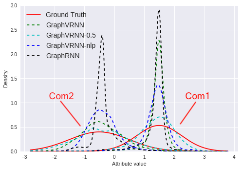
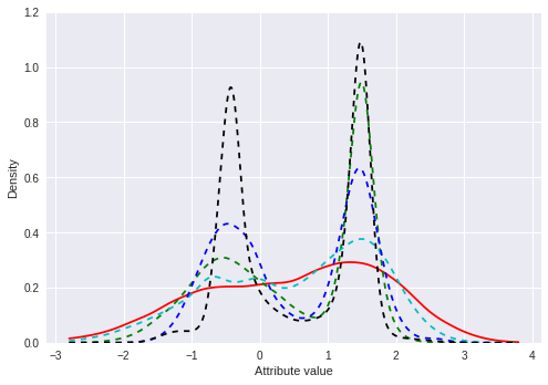
We show the density plot of the generated attributes in each community in Figure 2, and denote the two communities as Com1 and Com2. One can see that GraphRNN simply generates all the attributes around the modes since the model is trained to maximize the likelihood objective with deterministic recurrent networks, lacking the ability to capture the uncertainty faithfully. On the other hand, GraphVRNN approximates the distribution of Com1 well, while giving reasonable approximates of Com2 (Figure 2(left)). We further report the Earth Mover’s distance (the lower the better) between the generated attribute distribution and the true distribution for (1) each community and (2) the whole graph (denoted as All), along with the MMD metric in Table 2. It can be seen that GraphRNN yields good results on learning the graph structures, but approximates the attribute distributions poorly. On the other hand, GraphVRNN shows superior results in the attribute modeling task. Comparing GraphVRNN to GraphVRNN-nlp, the results imply that overall the learned prior network helps capture the attribute distribution better. Additionally, has a crucial impact on attribute generation task. Relaxing to 0.5 allows the prior to be more flexible, improving the approximation on the attribute distribution of the whole graph (Figure 2(right)). To conclude, we show that, equipped with the learned prior network, GraphVRNN is capable of learning graph structures and attribute distributions simultaneously even for large-scale graphs. We include all qualitative results in Appendix C.
4 Conclusion
We proposed GraphVRNN, a variational recurrent network for graph generation. Through modeling the probabilistic latent factors of the graph data, we show that GraphVRNN is capable of modeling the intricate and convoluted distribution of synthetic graph datasets. One future direction of this work is to experiment GraphVRNN in real-world applications (e.g. molecules generation, knowledge graph construction). In contrast to the artificially constructed dataset, the real-world data challenges the model to learn complex or even irregular patterns among both graph structure and attributes, which may necessitate the need of adopting strong priors [19]. We leave this direction for the future work.
References
- Chung et al. [2015] Junyoung Chung, Kyle Kastner, Laurent Dinh, Kratarth Goel, Aaron C Courville, and Yoshua Bengio. A recurrent latent variable model for sequential data. In NeurIPS, 2015.
- Dinh et al. [2017] Laurent Dinh, Jascha Sohl-Dickstein, and Samy Bengio. Density estimation using real nvp. In ICLR, 2017.
- Fabius and van Amersfoort [2015] Otto Fabius and Joost R van Amersfoort. Variational recurrent auto-encoders. In ICLR, 2015.
- Goodfellow et al. [2014] Ian Goodfellow, Jean Pouget-Abadie, Mehdi Mirza, Bing Xu, David Warde-Farley, Sherjil Ozair, Aaron Courville, and Yoshua Bengio. Generative adversarial nets. In NeurIPS, 2014.
- Hamilton et al. [2017] Will Hamilton, Zhitao Ying, and Jure Leskovec. Inductive representation learning on large graphs. In NeurIPS, 2017.
- Jin et al. [2018] Wengong Jin, Regina Barzilay, and Tommi Jaakkola. Junction tree variational autoencoder for molecular graph generation. In ICML, 2018.
- Kingma and Ba [2015] Diederik P Kingma and Jimmy Ba. Adam: A method for stochastic optimization. In ICLR, 2015.
- Kingma and Welling [2014] Diederik P Kingma and Max Welling. Auto-encoding variational bayes. In ICLR, 2014.
- Kipf and Welling [2016] Thomas N Kipf and Max Welling. Variational graph auto-encoders. NeurIPS Workshop, 2016.
- Kipf and Welling [2017] Thomas N Kipf and Max Welling. Semi-supervised classification with graph convolutional networks. In ICLR, 2017.
- Li et al. [2018] Yujia Li, Oriol Vinyals, Chris Dyer, Razvan Pascanu, and Peter Battaglia. Learning deep generative models of graphs. In ICLR, 2018.
- Liu et al. [2019] Jenny Liu, Aviral Kumar, Jimmy Ba, Jamie Kiros, and Kevin Swersky. Graph normalizing flows. arXiv preprint arXiv:1905.13177, 2019.
- Madjiheurem and Toni [2019] Sephora Madjiheurem and Laura Toni. Representation learning on graphs: A reinforcement learning application. In AISTATS, 2019.
- Mehrasa et al. [2019] Nazanin Mehrasa, Akash Abdu Jyothi, Thibaut Durand, Jiawei He, Leonid Sigal, and Greg Mori. A variational auto-encoder model for stochastic point processes. In CVPR, 2019.
- Norcliffe-Brown et al. [2018] Will Norcliffe-Brown, Stathis Vafeias, and Sarah Parisot. Learning conditioned graph structures for interpretable visual question answering. In NeurIPS, 2018.
- Simonovsky and Komodakis [2018] Martin Simonovsky and Nikos Komodakis. Graphvae: Towards generation of small graphs using variational autoencoders. In ICANN, 2018.
- Sohn et al. [2015] Kihyuk Sohn, Honglak Lee, and Xinchen Yan. Learning structured output representation using deep conditional generative models. In NeurIPS, 2015.
- Teney et al. [2017] Damien Teney, Lingqiao Liu, and Anton van den Hengel. Graph-structured representations for visual question answering. In CVPR, 2017.
- Xu et al. [2019] Haowen Xu, Wenxiao Chen, Jinlin Lai, Zhihan Li, Youjian Zhao, and Dan Pei. On the necessity and effectiveness of learning the prior of variational auto-encoder. arXiv preprint arXiv:1905.13452, 2019.
- You et al. [2018] Jiaxuan You, Rex Ying, Xiang Ren, William L. Hamilton, and Jure Leskovec. Graphrnn: generating realistic graphs with deep auto-regressive models. In ICML, 2018.
Appendix A Background
A.1 GraphRNN
In GraphRNN, they focus on learning the distribution , the structural pattern of graphs without the attribute matrix . They proposed to reformulate the learning task as a sequence prediction problem. First, they map into a sequence with a breadth-first search (BFS):
| (4) |
where is a sequence under a possible node permutation generated by the BFS policy, and is the adjacency vector between node and its previously generated nodes. The assumption here is that BFS would map the neighboring nodes of within steps, and therefore omits the need of checking all the other nodes. The learning target then becomes :
| (5) | ||||
| (6) |
Equation 6 is factroized and modeled by a node-level and an edge-level RNN that keeps track of the information on previously generated adjacency vectors and edges respectively for node , and is a function that maps sequence back to a graph. The two RNNs predict the adjacency vector sequentially, and put together the predicted to generate the adjacency matrix as the final output.
A.2 Variational Autoencoder
Variational Autoencoder (VAE) [8] is a probabilistic generative model with a latent variable which can be used to approximate likelihood of data . The generation is performed by sampling from a latent space using the prior distribution . The sampled code is next decoded through a conditional distribution to reconstruct . Given this, the likelihood of data can be obtained as . However, this is interactable to compute. Thus, is approximated by a variational lower bound as bellow:
| (7) |
This formulation gives an autoencoder structure composed of an inference network and a generation network to encode and decode data. In the inference network, a proposal posterior is learned instead of the intractable true posterior to sample . This sample is next decoded through the generation module to reconstruct . denotes the Kullback-Leibler (KL) divergence between the prior and the proposal distribution. This can be also interpreted as a regularizer for the reconstruction loss.
In vanilla VAE, the proposal posterior is modeled as diagonal normal distribution and the prior is the standard normal distribution . This gives an analytical solution for the KL divergence. To train this VAE, and are modeled as neural networks, and the parameters and are learned by optimizing 7 using the re-parameterization trick [8]
Conditional VAE (CVAE) [17] is an extension to VAE which approximates the conditional distribution . The variational lower bound for CVAE is defined as:
| (8) |
Appendix B Model Details
B.1 Network Modules
For nodel-level RNN and edge-level RNN, we uses a 4-layer GRU unit with a hidden size of 128 and 16 respectively as in [20]. The prior and posterior networks both consist of a 3-layer MLP with ReLU non-linearity for hidden layers, and mapped the output of node-level RNN into a 64-dim latent vector . Similarly, the attribute decoder adopts a 3-layer MLP network, and take as input the , the hidden state of node-level RNN and the predicted adjacency vector to generate the note attribute . We use binary cross-entropy and mean squared error as the reconstruction losses for and respectively. For small size graph, we follow the practice in [20] to half the hidden size of the node-level RNN.
For GraphRNN, the input of attribute decoder is simply and .
B.2 Experiment Settings
We use the official GraphRNN Github111GraphRNN: https://github.com/JiaxuanYou/graph-generation repository provided by the authors for training the baseline models, generating the synthetic dataset set and evaluating the MMD metric. We follow the same hyperparameter settings suggested in [20]: in all experiments, we use Adam optimizer [7] with batch size 32 (32 graphs per batch). The learning rate is set to 0.001, and decay it by 0.3 at training steps 12800 and 32000. In all experiments, we only consider or , without doing any hyperparameter search.
Appendix C Qualitative Result
| Ego-small | ||
 |
 |
 |
| Com-small | ||
 |
 |
 |
| Com-mix | ||
 |
 |
 |
| Com-attr | ||
 |
 |
 |
| (a) Training samples | (b) GraphVRNN | (c) GraphRNN |
C.1 Dataset details
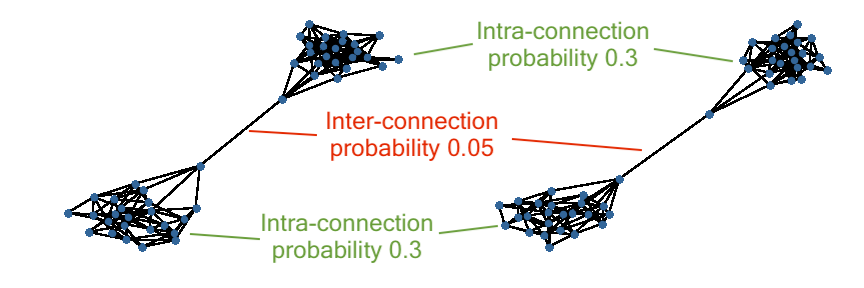
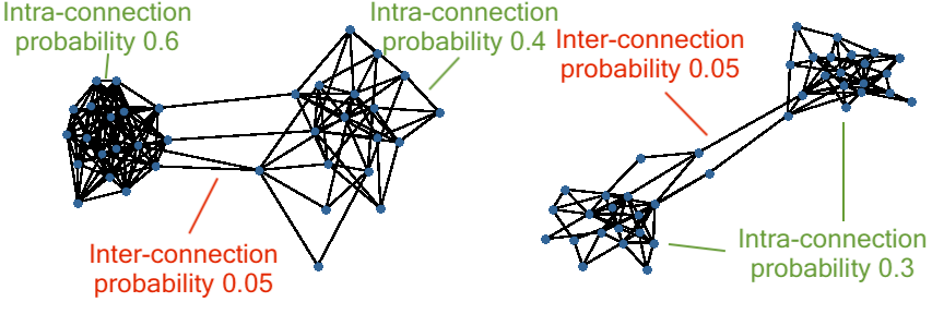
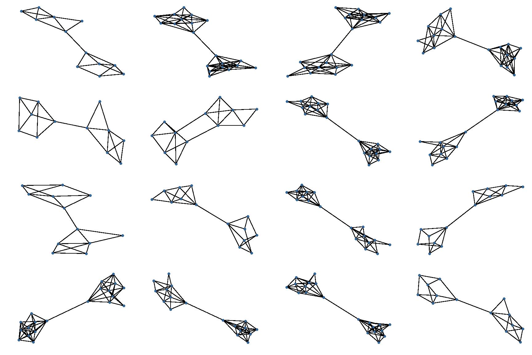
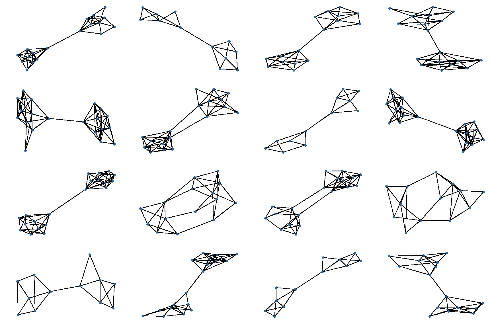
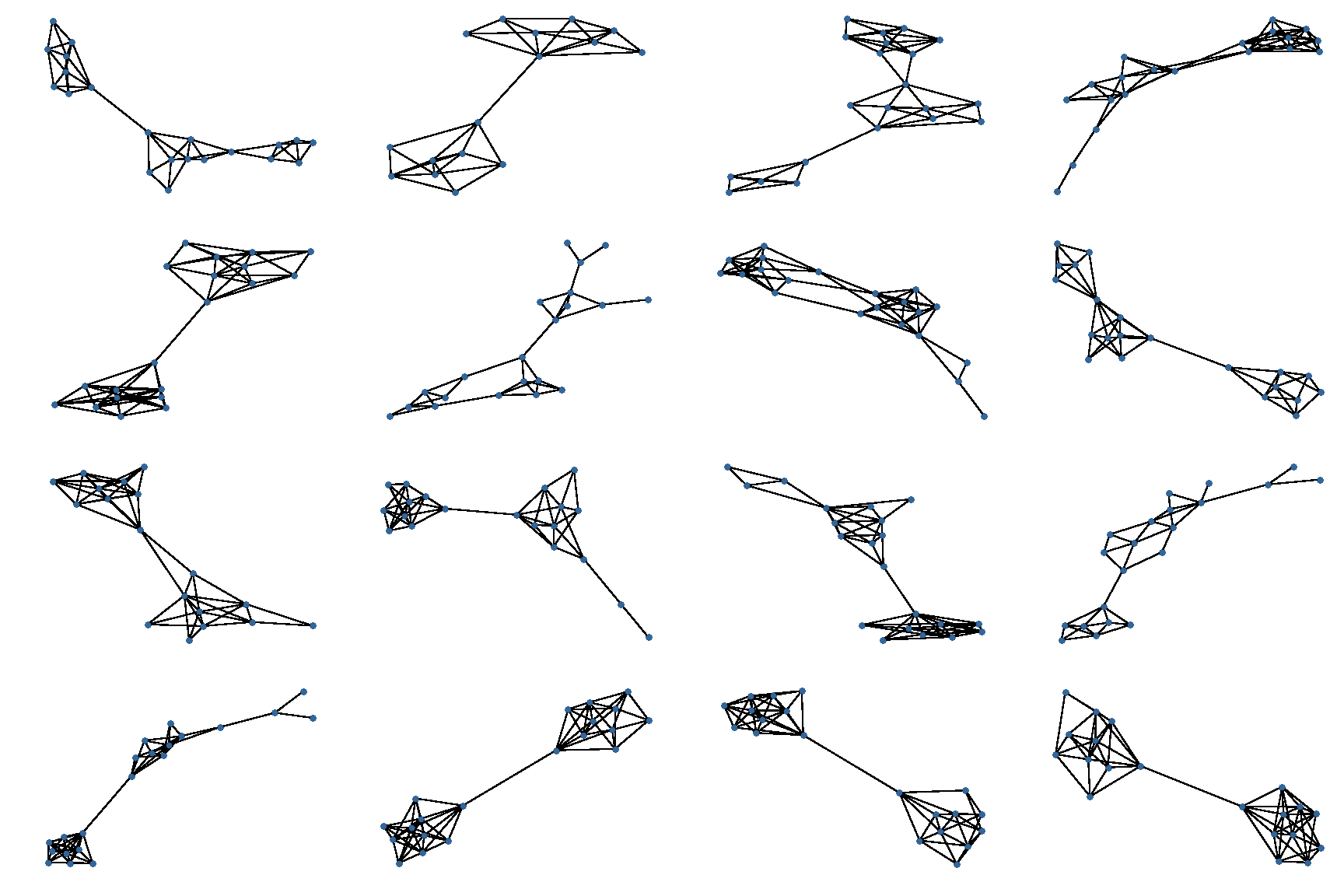
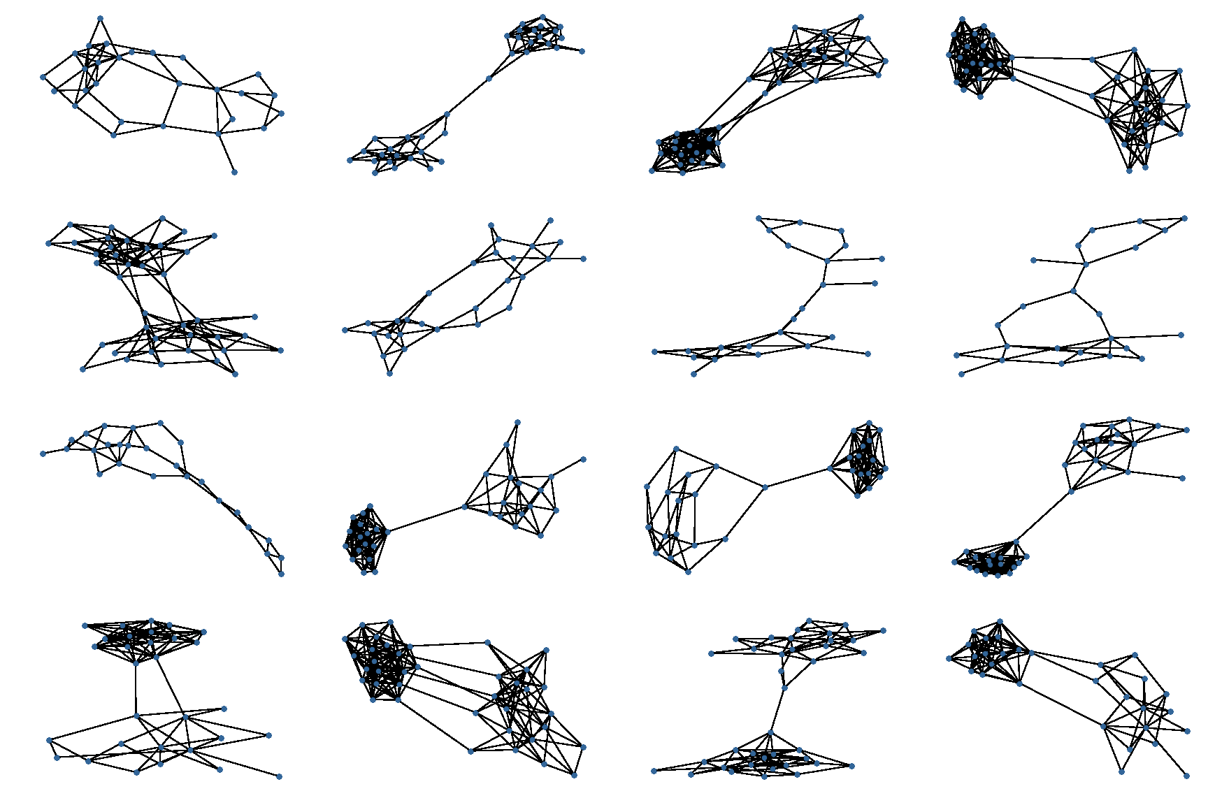
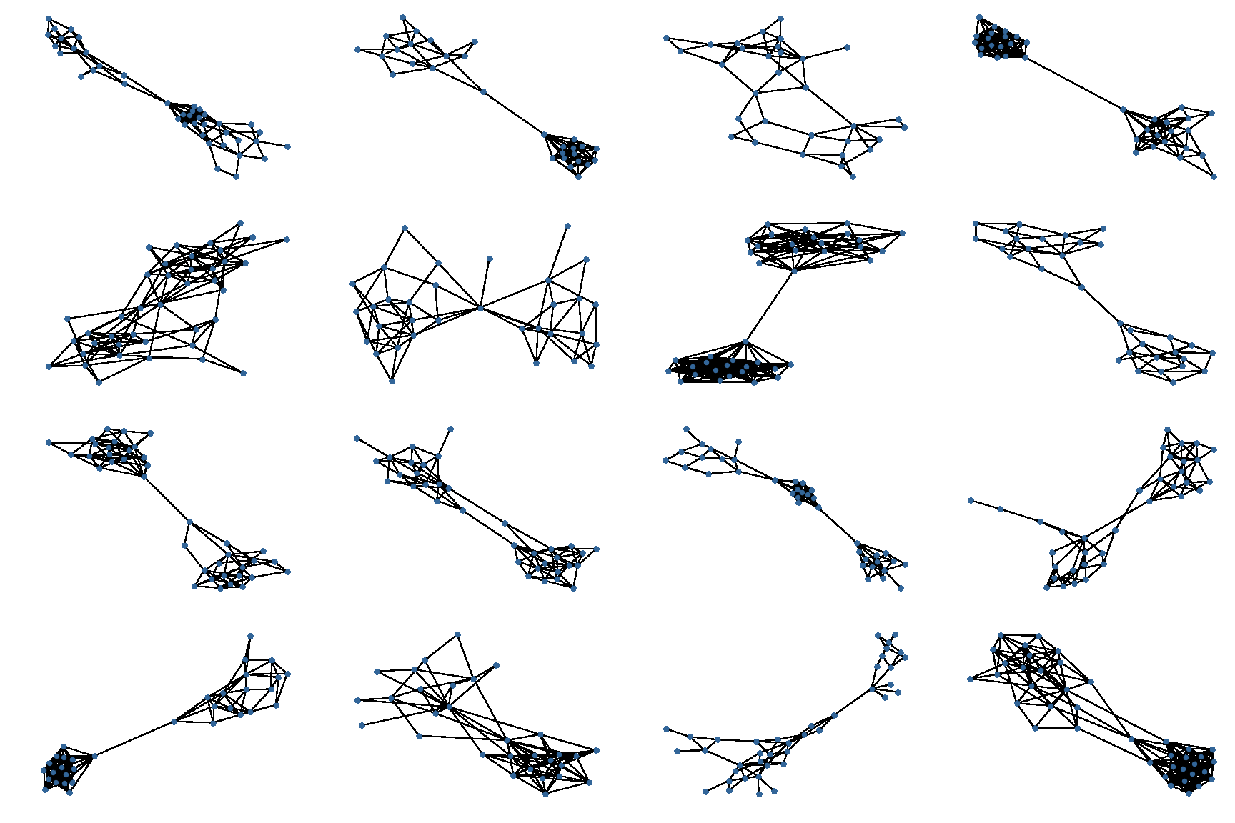
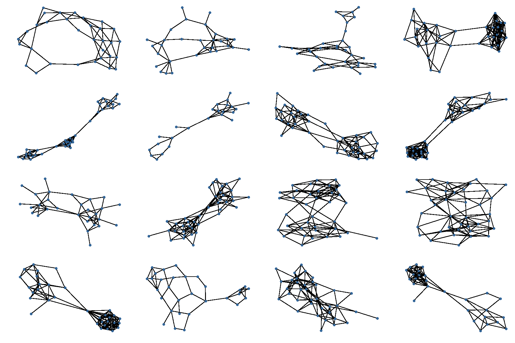
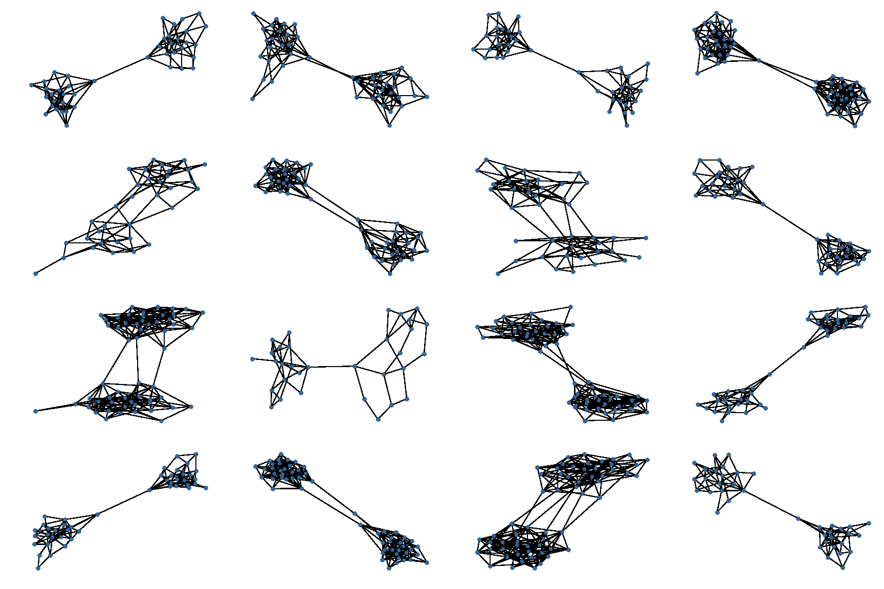
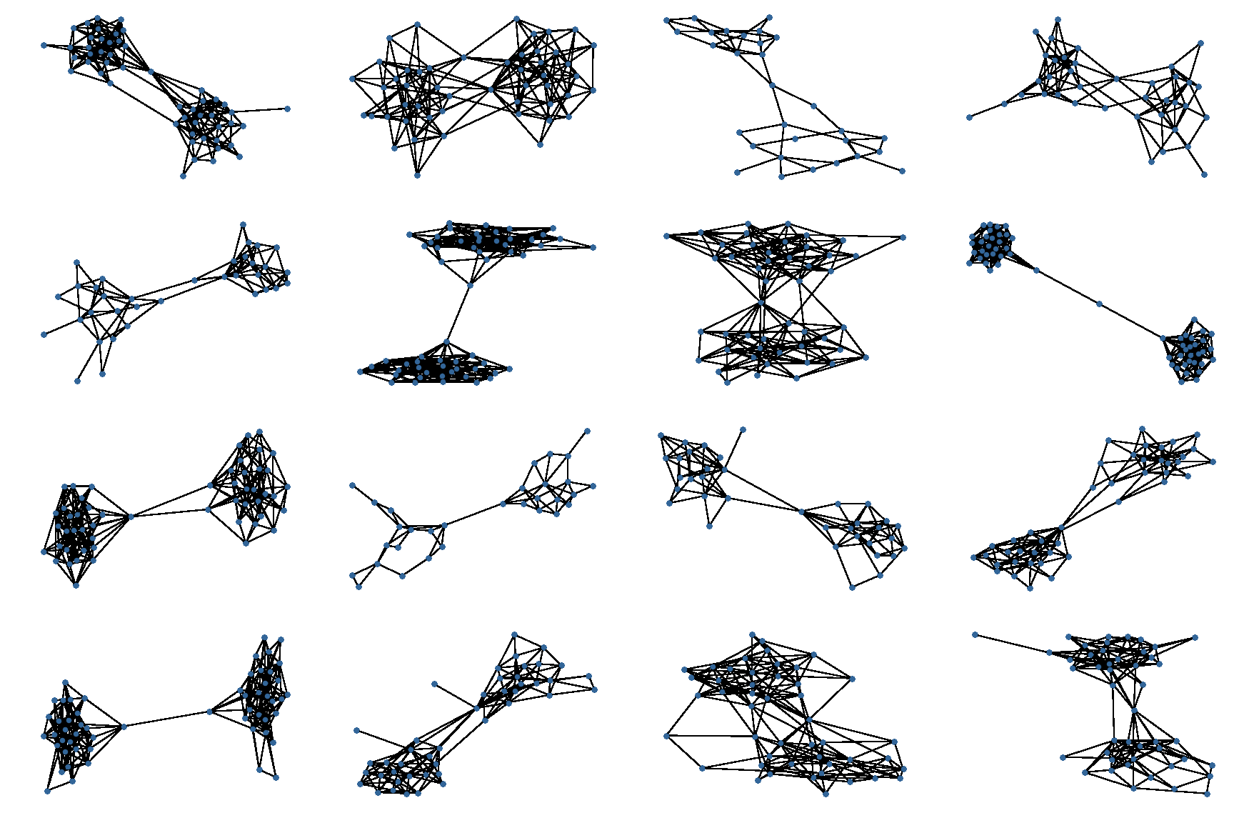
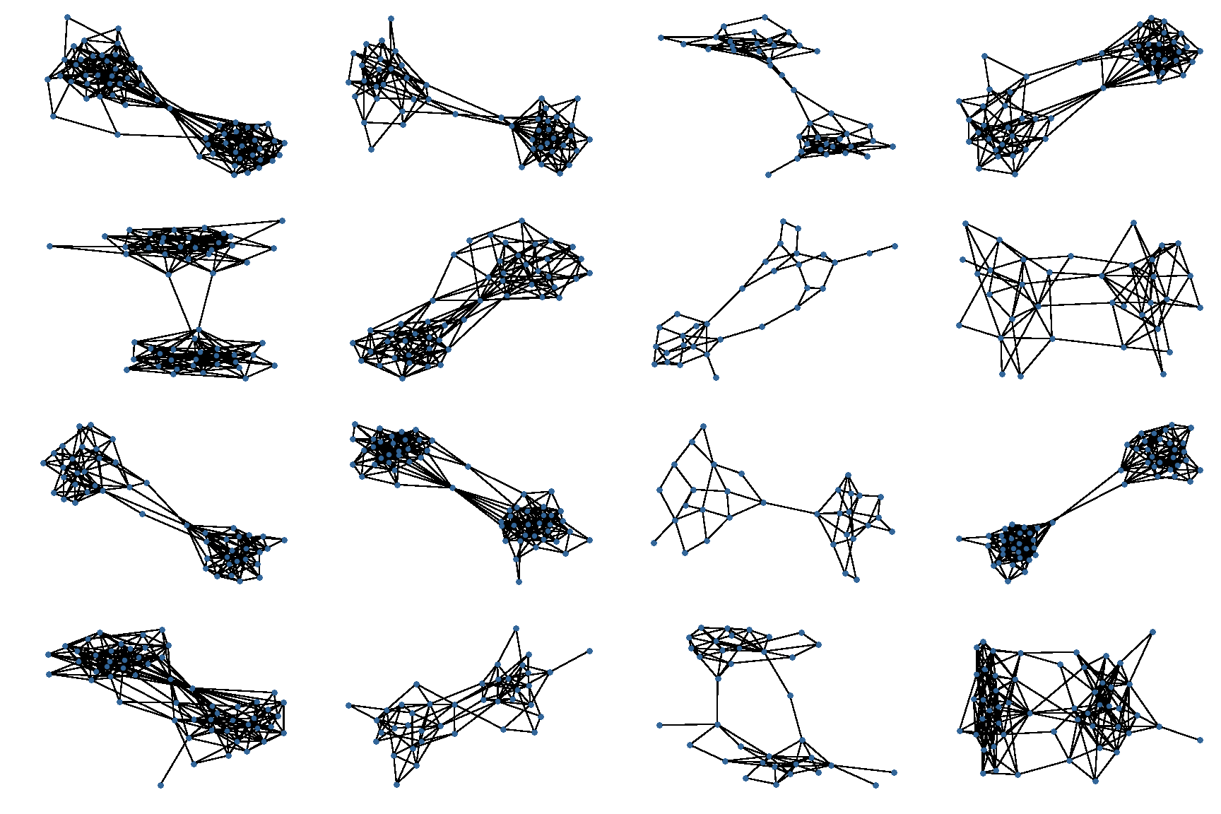
In Figure 3, we show two illustrative examples of the 2-community datasets (namely Com-small, Com-mix and Com-attr) considered in Section 3. For these datasets, each graph consists of two communities. The edge connection within each community is determined by the intra-connection probability, while the connection across the two communities is determined by the inter-connection probability. For Com-attr, the two communities have the same intra-connection probability 0.3 (and 0.7 for Com-small dataset), as shown in Figure 3(a). On the other hand, the intra-connection probability is not necessarily the same. As illustrated in Figure 3(b), there exists two kinds of graphs in Com-mix: one with different intra-connection probabilities for the two communities (0.6 and 0.4), and the other with the same intra-connection probabilities.
C.2 Qualitative results
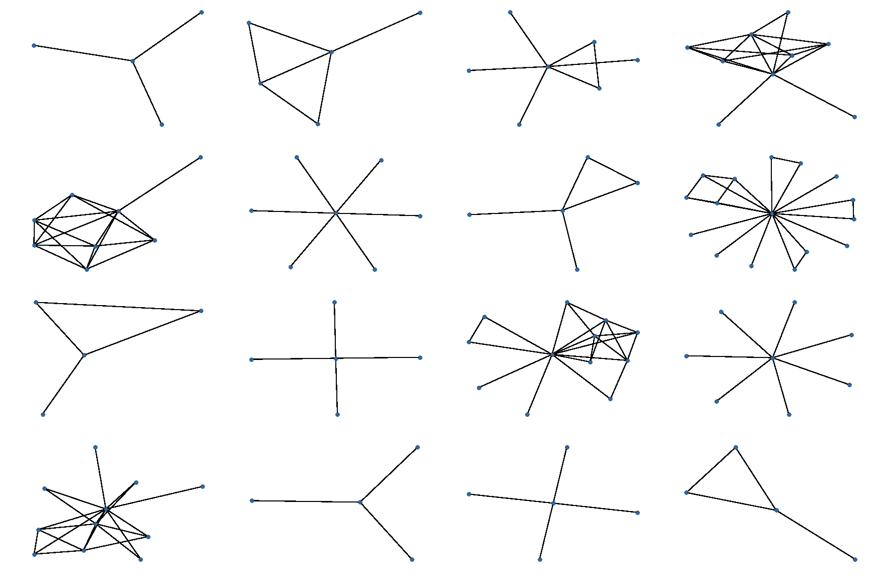
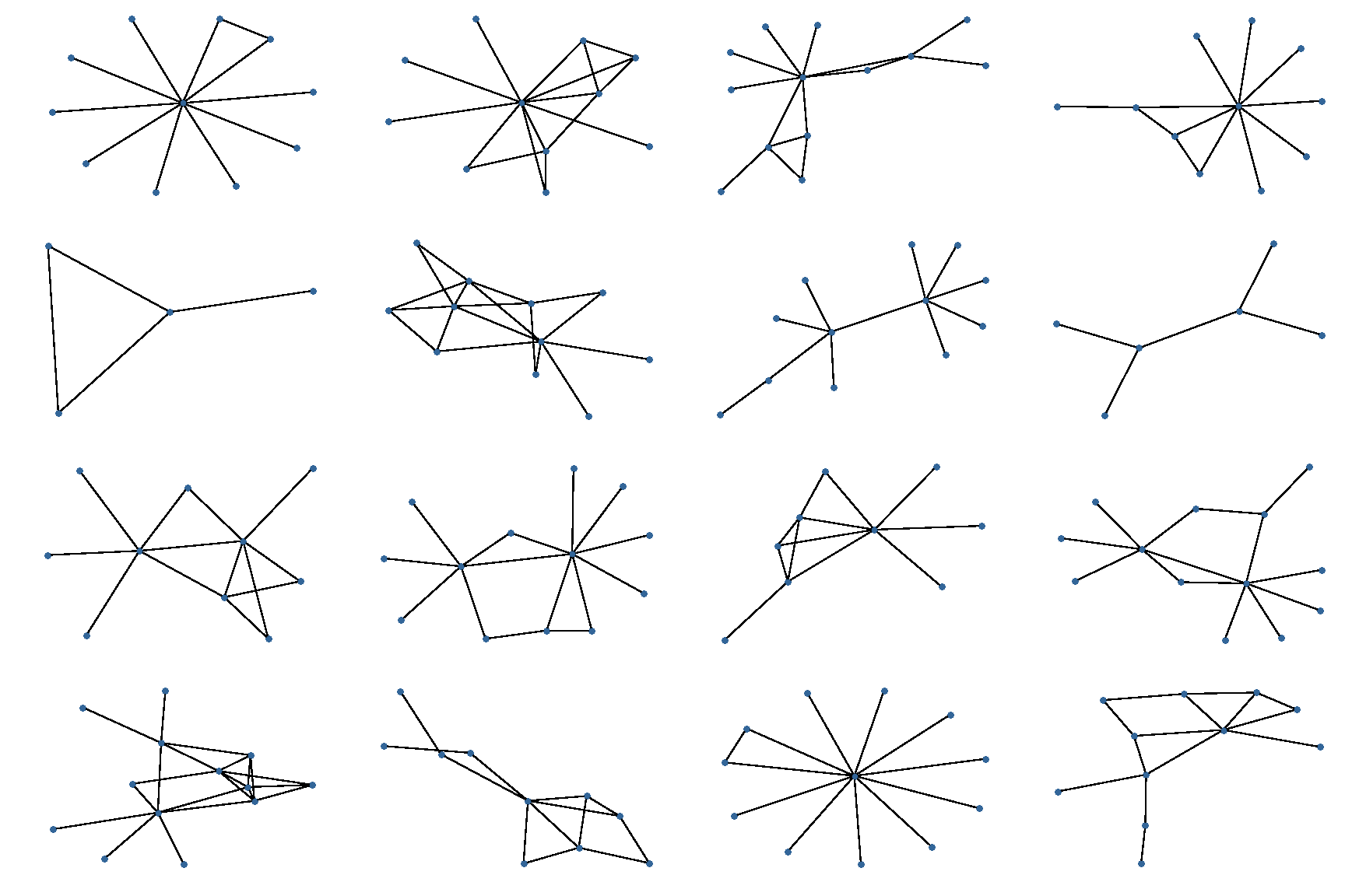
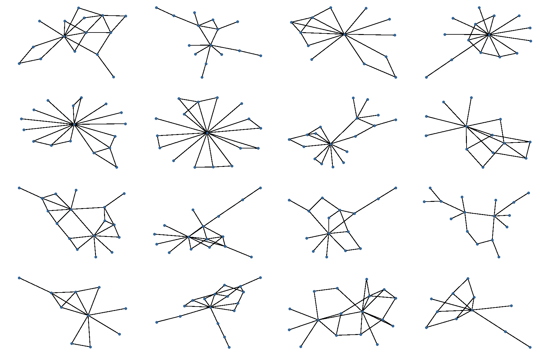
We present the graphs generated from GraphVRNN and GraphRNN in Figure 4. For each dataset, we pick the best model out of the 5 training runs, and randomly select 16 graphs from the generated samples.