Machine learning strategies for path-planning microswimmers in turbulent flows
Abstract
We develop an adversarial-reinforcement learning scheme for microswimmers in statistically homogeneous and isotropic turbulent fluid flows, in both two (2D) and three dimensions (3D). We show that this scheme allows microswimmers to find non-trivial paths, which enable them to reach a target on average in less time than a naïve microswimmer, which tries, at any instant of time and at a given position in space, to swim in the direction of the target. We use pseudospectral direct numerical simulations (DNSs) of the 2D and 3D (incompressible) Navier-Stokes equations to obtain the turbulent flows. We then introduce passive microswimmers that try to swim along a given direction in these flows; the microswimmers do not affect the flow, but they are advected by it. Two, non-dimensional, control parameters play important roles in our learning scheme: (a) the ratio of the microswimmer’s bare velocity and the root-mean-square (rms) velocity of the turbulent fluid; and (b) the product of the microswimmer-response time and the rms vorticity of the fluid. We show that the average time required for the microswimmers to reach the target, by using our adversarial-learning scheme, eventually reduces below the average time taken by microswimmers that follow the naïve strategy.
I Introduction
Machine-learning techniques and advances in computational facilities have led to significant improvements in obtaining solutions to optimization problems, e.g., to problems in path planning and optimal transport, referred to in control systems as Zermelo’s navigation problem Zermelo . With vast amounts of data available from experiments and simulations in fluid dynamics, machine-learning techniques are being used to extract information that is useful to control and optimize flows ML_FM . Recent studies include the use of reinforcement learning, in fluid-flow settings, e.g., (a) to optimise the soaring of a glider in thermal currents Soaring and (b) the development of an optimal scheme in two- (2D) and three-dimensional (3D) fluid flows that are time independent PRL ; 3D . Optimal locomotion, in response to stimuli, is also important in biological systems ranging from cells and micro-organisms Dusenbery ; Durham ; Michalec to birds, animals, and fish Fish ; such locomotion is often termed taxis Barrows .
It behooves us, therefore, to explore machine-learning strategies for optimal path planning by microswimmers in turbulent fluid flows. We initiate such a study for microswimmers in 2D and 3D turbulent flows. In particular, we consider a dynamic-path-planning problem that seeks to minimize the average time taken by microswimmers to reach a given target, while moving in a turbulent fluid flow that is statistically homogeneous and isotropic. We develop a novel, multi-swimmer, adversarial--learning algorithm to optimise the motion of such microswimmers that try to swim towards a specified target (or targets). Our adversarial--learning approach ensures that the microswimmers perform at least as well as those that adopt the following naïve strategy: at any instant of time and at a given position in space, a naïve microswimmer tries to point in the direction of the target. We examine the efficacy of this approach as a function of the following two dimensionless control parameters: (a) , where the microswimmer’s bare velocity is and the the turbulent fluid has the root-mean-square velocity ; and (b) , where is the microswimmer-response time and the rms vorticity of the fluid. We show, by extensive direct numerical simulations (DNSs), that the average time , required by a microswimmer to reach a target at a fixed distance, is lower, if it uses our adversarial--learning scheme, than if it uses the naïve strategy.
II Background flow and microswimmer dynamics
For the low-Mach-number flows we consider, the fluid-flow velocity satisfies the incompressible Navier-Stokes (NS) equation. In two dimensions (2D), we write the NS equations in the conventional vorticity-stream-function form, which accounts for incompressibility in 2D RP_Review :
| (1) |
here, is the fluid velocity, is the kinematic viscosity, is the coefficient of friction (present in 2D, e.g., because of air drag or bottom friction) and the vorticity , which is normal to in 2D. The 3D incompressible NS equations are
| (2) |
is the pressure and the density of the incompressible fluid is taken to be ; the large-scale forcing (large-scale random forcing in 2D) or (constant energy injection in 3D) maintains the statistically steady, homogeneous, and isotropic turbulence, for which it is natural to use periodic boundary conditions.
We consider a collection of passive, non-interacting microswimmers in the turbulent flow; and are the position and swimming direction of the microswimmer. Each microswimmer is assigned a target located at . We are interested in minimizing the time required by a microswimmer, which is released at a distance from its target, to approach within a small distance of this target. The microswimmer’s position and swimming direction evolve as follows Pedley :
| (3) | |||||
| (4) |
here, we use bi-linear (tri-linear) interpolation in 2D (3D) to determine the fluid velocity at the microswimmer’s position from eq. 2; is the swimming velocity, is the time-scale associated with the microswimmer to align with the flow, and is the control direction. Equation 4 implies that tries to align along . We define the following non-dimensional control parameters: , where is the root-mean-square () fluid flow velocity, and , where ; denotes the root-mean-square vorticity.
III Adversarial -learning for smart microswimmers
Designing a strategy consists in choosing appropriately the control direction , as a function of the instantaneous state of the microswimmer, in order to minimize the mean arrival time . To develop a tractable framework for -learning, we use a finite number of states by discretizing the fluid vorticity at the microswimmer’s location into 3 ranges of values labelled by and the angle , between and , into 4 ranges , as shown in fig 1. The choice of is then reduced to a map from to an action set, , which we also discretize into the following four possible actions: , where is the unit vector pointing from the swimmer to its target and . Therefore, for the naïve strategy , . This strategy is optimal if : Microswimmers have an almost ballistic dynamics and move swiftly to the target. For , vortices affect the microswimmers substantially, so we have to develop a nontrivial -learning strategy, in which is a function of and .
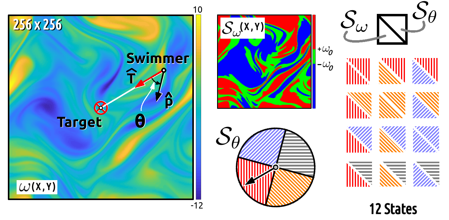
In our -learning scheme, we assign a quality value to each state-action binary relation of microswimmer as follows: , where and ; and we use the -greedy method Watkins (with parameter ), in which the control direction is chosen from the probability distribution , where and is the Dirac delta function. At each iteration, is calculated as above and the microswimmer evolution is performed by using eqs. 3 and 4. In the canonical -learning approach, during the learning process, each of the ’s are evolved by using the Bellman equation Sutton below, whenever there is a state change, i.e., :
| (5) |
where and are learning parameters that are set to optimal values after some numerical exploration (see tab. 1), and is the reward function. For the path-planning problem we define , where . According to eq. 5, any for which is positive can be a solution, and there exist many such solutions that are sub-optimal compared to the naïve strategy.
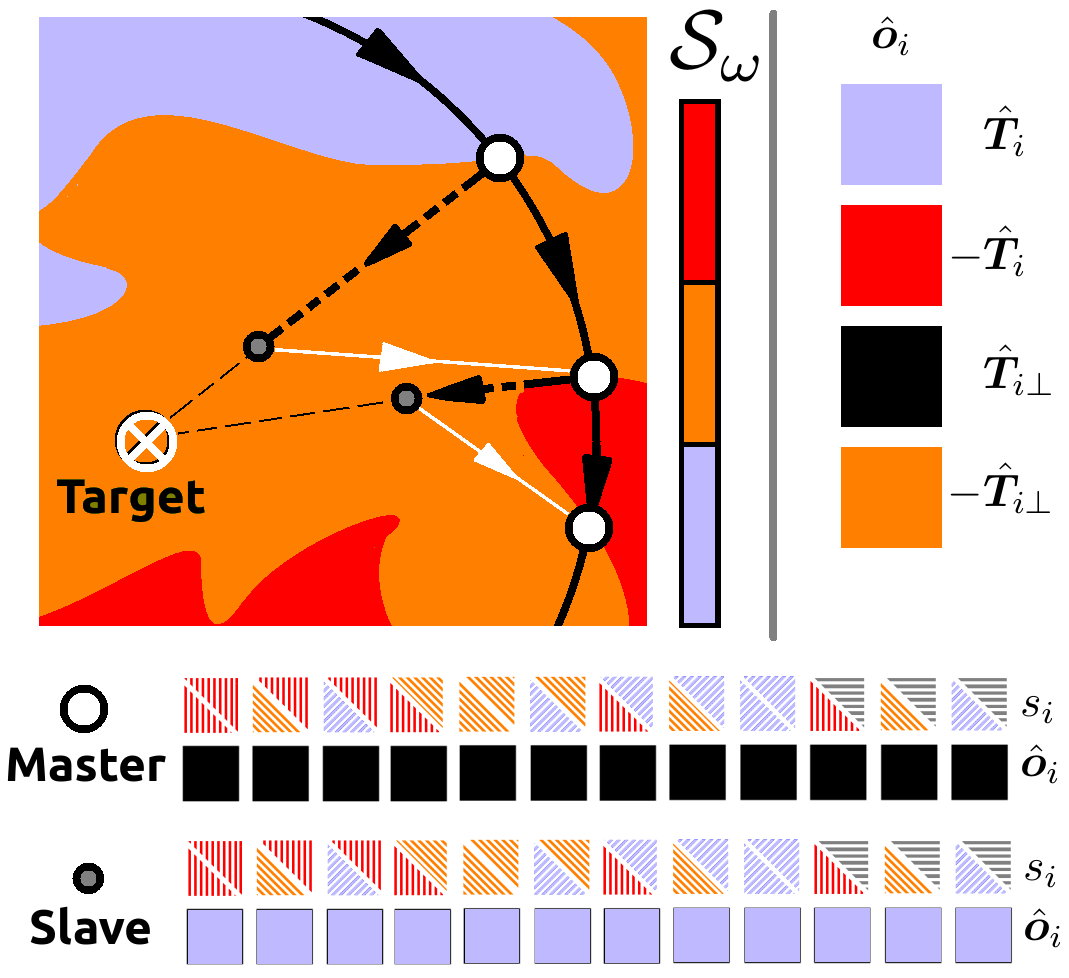
To reduce the solution space, we propose an adversarial scheme: Each microswimmer, the master, is accompanied by a slave microswimmer, with position , that shares the same target at , and follows the naïve strategy, i.e., . Now, whenever the master undergoes a state change, the corresponding slave’s position and direction are re-initialized to that of the master, i.e., if , then and (see fig. 2). Then the reward function for the master microswimmer is given by ; i.e., only those changes that improve on the naïve startegy are favored.
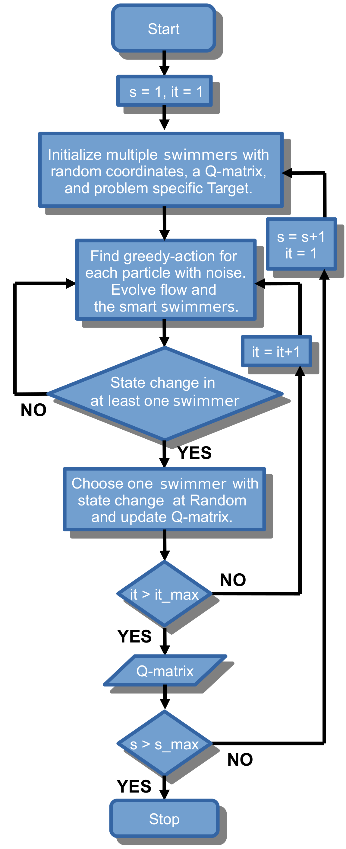
In the conventional -learning approach Watkins ; Survey , the matrices of each microswimmer evolve independently; this matrix is updated only after a state change, so a large number of iterations are required for the convergence of . To speed-up this learning process, we use the following multi-swimmer, parallel-learning scheme: all the microswimmers share a common matrix, i.e., . At each iteration, we choose one microswimmer at random, from the set of microswimmers that have undergone a state change, to update the corresponding element of the matrix (flow chart in Appendix A); this ensures that the matrix is updated at almost every iteration and so it converges rapidly.
IV Numerical simulation
We use a pseudospectral DNS canuto ; pramanareview , with the dealiasing rule to solve eqs. 1 and 2. For time marching we use a third-order Runge-Kutta scheme in 2D and the exponential Adams-Bashforth time-integration scheme in 3D; the time step is chosen such that the Courant-Friedrichs-Lewy (CFL) condition is satisfied. Table 2 gives the parameters for our DNSs in 2D and 3D, such as the number of collocation points and the Taylor-microscale Reynolds numbers , where the Taylor microscale .
| 2D | 3D | |
|---|---|---|
IV.1 Naïve microswimmers
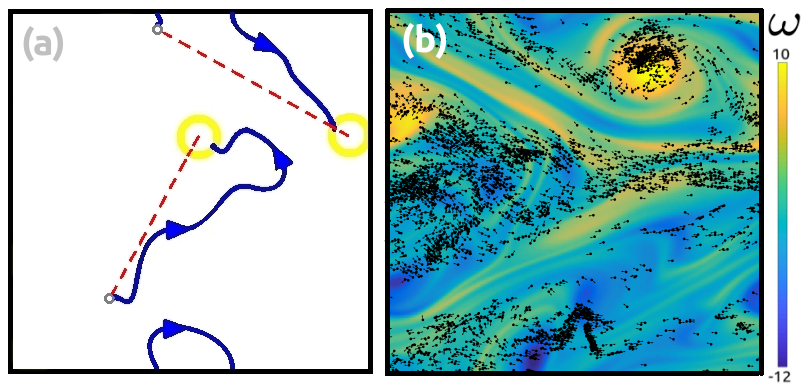
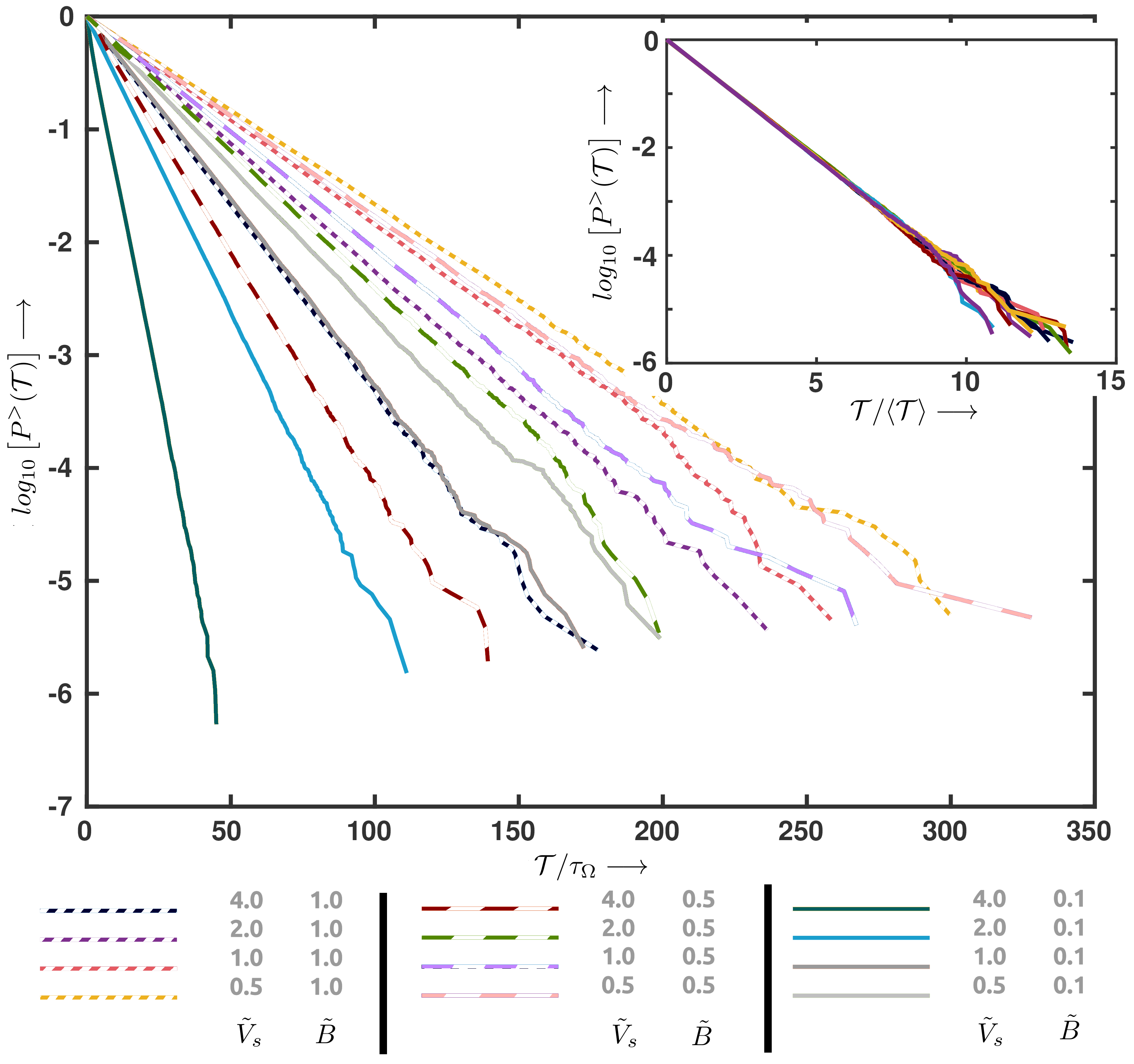
The average time taken by the microswimmers to reach their targets is (see fig. 3). If is the unit vector pointing from the microswimmer to the target, then for we expect the naïve strategy, i.e., , to be the optimal one. For , we observe that the naïve strategy leads to the trapping of microswimmers (fig. 3(b)) and gives rise to exponential tails in the arrival-time () probability distribution function (PDF); in fig. 4 we plot the associated complementary cumulative distribution function (CCDF) , where is the probability of particle arrival in the time interval and is the time since initialization of the microswimmer. As a consequence of trapping, is dominated by the exponential tail of the distribution, as can be seen from fig. 4.
IV.2 Smart microswimmers
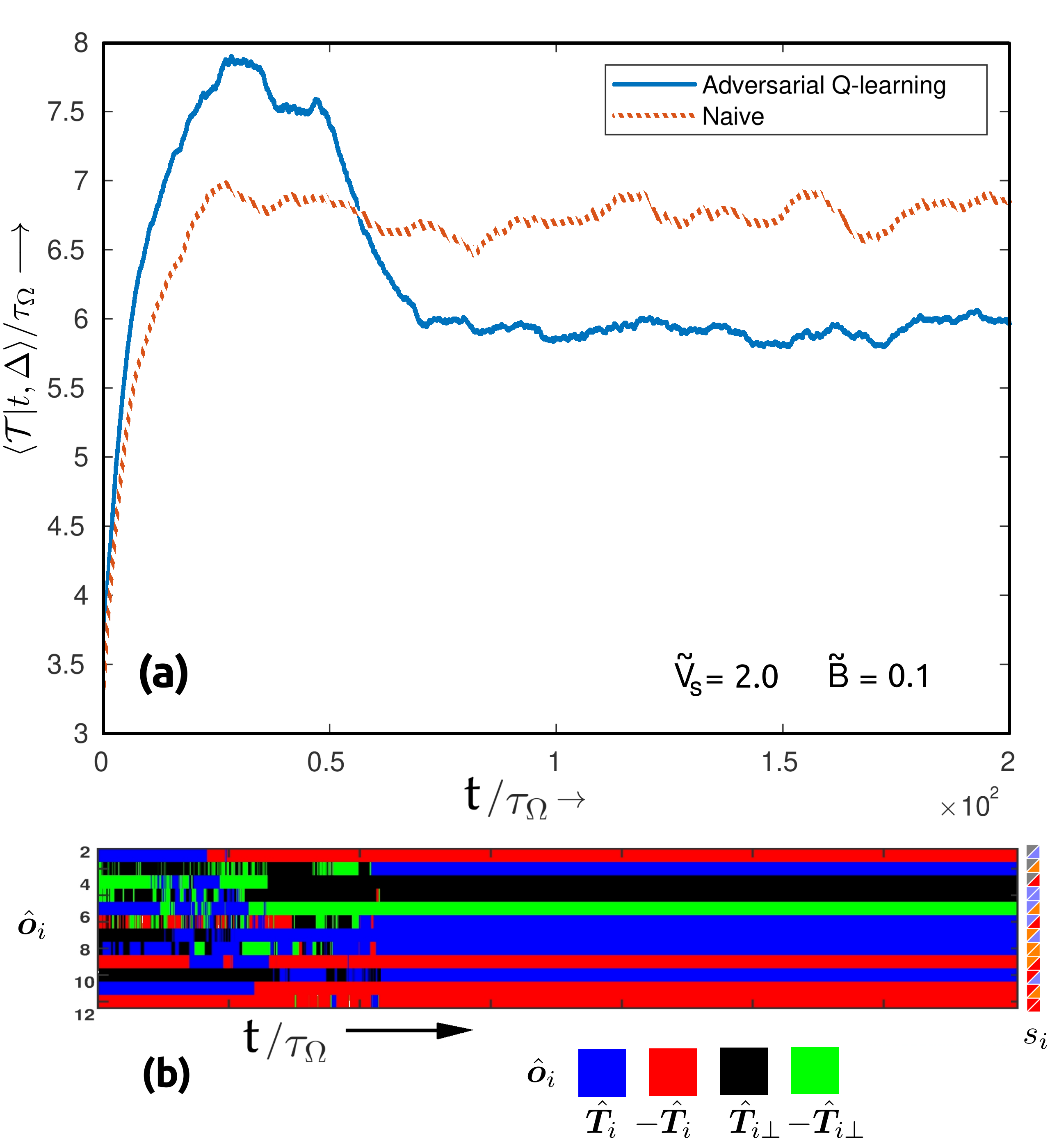
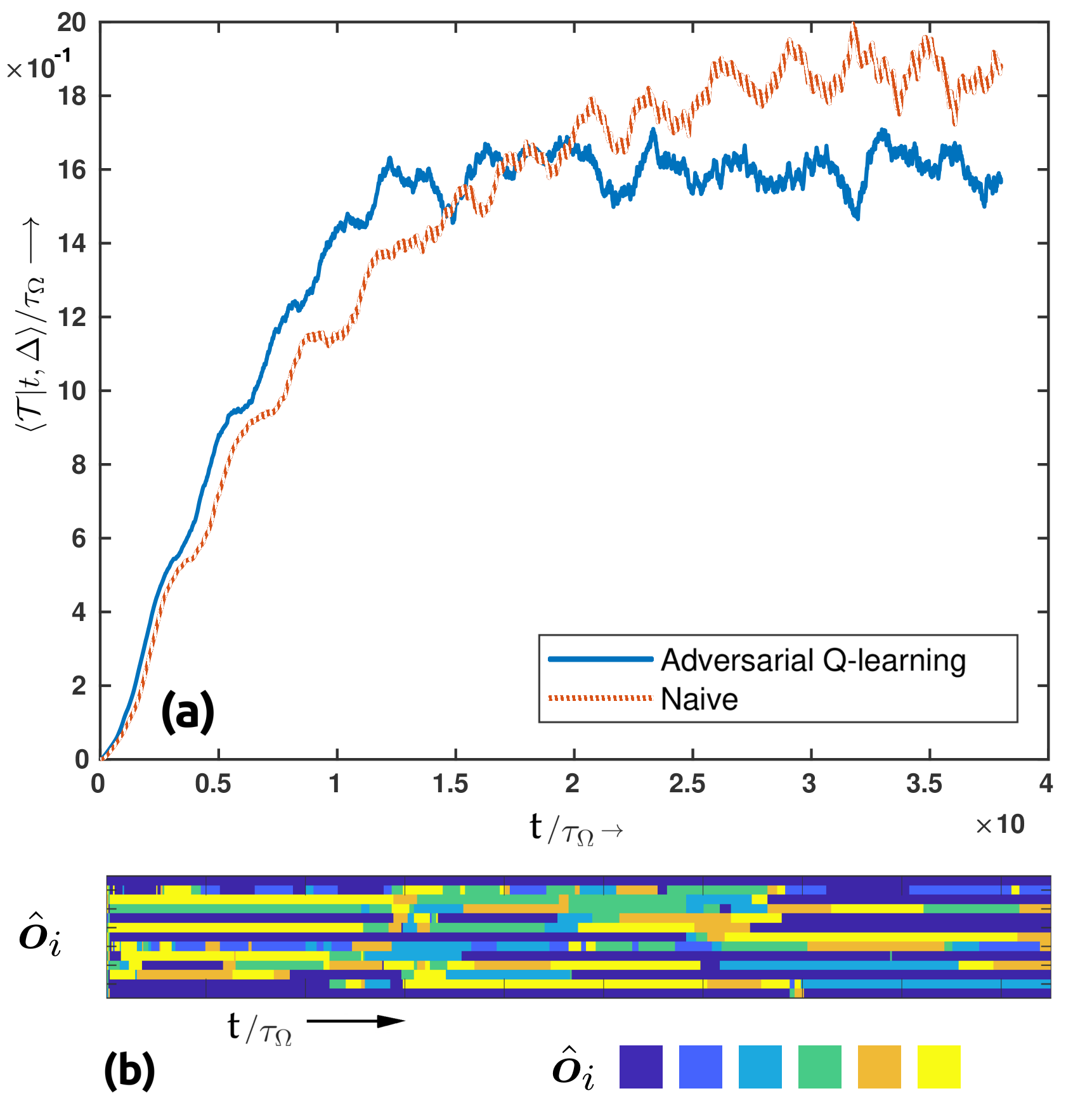
In our approach, the random initial positions of the microswimmers ensures that they explore different states without reinitialization for each epoch. Hence, we present results with 10000 microswimmers, for a single epoch. In our single-epoch approach, the control map reaches a steady state once the learning process is complete (fig. 5(b)). We would like to clarify here that, in our study, the training is performed in the fully turbulent time-dependent flow; even though this is more difficult than training in a temporally frozen flow, the gains, relative to the naïve strategy, justify this additional level of difficulty.
We use the adversarial -learning approach outlined above (parameter values in tab. 1) to arrive at the optimal scheme for path-planning in a 2D turbulent flow. To quantify the performance of the smart microswimmers, we introduce equal numbers of smart (master-slave pairs) and naïve microswimmers into the flow. The scheme presented here pits -learning against the naïve strategy and enables the adversarial algorithm to find a strategy that can out-perform the naïve one. (Without the adversarial approach, the final strategy that is obtained may end up being sub-optimal.)
V Results
The elements of evolve during the initial-training stage, so also evolves in time until the system reaches a statistically steady state (in which the elements of do not change). Hence, also changes during the initial-training stage; to capture this time dependence, we define , where is the time taken by the microswimmer, since its intialization, to arrive at its target at the time instant and is the number of microswimmers that reach their targets at time instant . We find that shows large fluctuations; so we average it over a time window and define . The initial growth in arises because . The plots in figs. 5(a) and 7 show the time evolution of for the smart and naïve microswimmers. Note that becomes a constant, for large , in fig. 5(b); this implies that the elements of have settled down to their steady-state values.
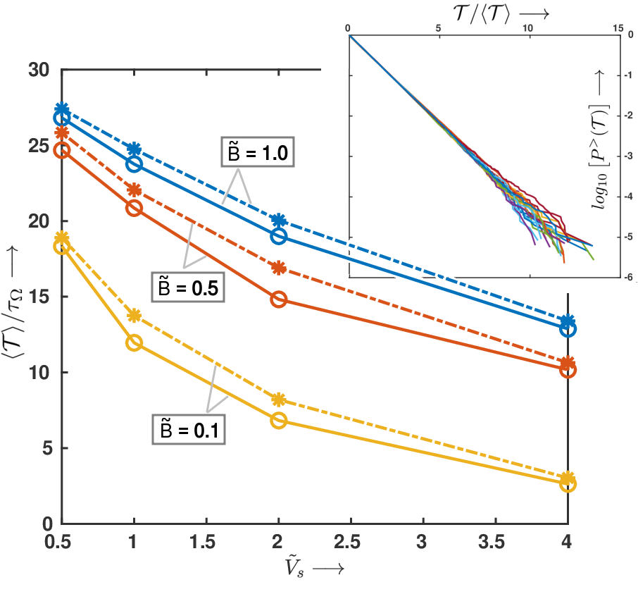
Figures 5(a), and 5(b) show the evolution of and , respectively, for the naïve strategy and our adversarial--learning scheme. After the initial learning phase, the -learning algorithm explores different , before it settles down to a steady state. It is not obvious, a priori, if there exists a stable, non-trivial, optimal strategy, for microswimmers in turbulent flows, that could out-perform the naïve strategy. The plot in fig. 6 shows the improved performance of our adversarial--learning scheme over the naïve strategy, for different values of and ; in these plots we use , so that the initial transient behavior in learning is excluded. The inset in fig. 6 shows that has an exponential tail, just like the naïve scheme in fig. 4, which implies the smart microswimmers also get trapped; but a lower value of implies they are able to escape from the traps faster than microswimmers that employ the naïve strategy. Note that the presence of a possible noise in the measurement of the discrete vorticity should not change our findings because of the coarse discretization we use in defining the states.
In a 3D turbulent flow, we also obtain such an improvement, with our adversarial -learning approach, over the naïve strategy. The details about the 3D flows, parameters, and the definitions of states and actions are given in Appendix B. In fig. 7 we show a representative plot, for the performance measure, which demonstrates this improvement in the 3D case (cf. fig. 5 for a 2D turbulent flow).
VI Conclusions
We have shown that the generic -learning approach can be adopted to solve control problems arising in complex dynamical systems. In HJB , global information of the flows has been used for path-planning problems in autonomous-underwater-vehicles navigation to improve their efficiency, based on the Hamilton-Jacobi-Bellmann approach. In contrast, we present a scheme that uses only the local flow parameters for the path planning.
The flow parameters (tab. 2) and the learning parameters (tab. 1) have a significant impact on the performance of our adversarial--learning method. Even the choice of observables that we use to define the states can be changed and experimented with. Furthermore, the discretization process can be eliminated by using deep-learning approaches, which can handle continuous inputs and outputs Deep_Q . Our formulation of the optimal-path-planning problem for microswimmers in a turbulent flow is a natural starting point for detailed studies of control problems in turbulent flows.
VII Discussion
We were made aware of BB during the writing of this manuscript, where they tackle the problem using an Actor-Critic reinforcement learning scheme.
We contrast, below, our reinforcement- learning approach with that of Ref. BB .
-
•
Reference BB uses 900 discrete states, which are defined based on the approximate location of the microswimmer. By contrast, our scheme uses only the local vorticity (), at the position of the microswimmer, and the orientation (); after discretization, we retain only 12 states. In analogy with navigation parlance, Ref. BB uses a GPS and our approach uses a light-house along with a local-vorticity measurement.
-
•
In Ref. BB , the states are sensed periodically and the elements of are updated at every sensing instant. In constrast, we monitor the states continuously and update the elements of only when there is a state change. If the periodicity of sensing is smaller than the rate of change in states of the microswimmer, both schemes should show similar convergence behaviors.
-
•
Reference BB uses a conventional, episode-based training approach, which is sequential, whereas we use multiple microswimmers to perform parallel training.
-
•
Reference BB uses an actor-critic approach, whereas we use an adversarial-learning method.
Acknowledgements.
We thank DST, CSIR (India), BRNS, and the Indo-French Centre for Applied Mathematics (IFCAM) for support.References
- (1) E. Zermelo Über das navigationsproblem bei ruhender oder veränderlicher windverteilung, ZAMM-Journal of Applied Mathematics and Mechanics/Zeitschrift für Angewandte Mathematik und Mechanik 11(2):114–124 (1931).
- (2) S. Brunton, B. Noack, P. Koumoutsakos, Machine Learning for Fluid Mechanics, arXiv e-prints p. arXiv:1905.11075.
- (3) G. Reddy, A. Celani, T. J. Sejnowski, M. Vergassola, Learning to soar in turbulent environments, Proceedings of the National Academy of Sciences 113(33):E4877–E4884 (2016).
- (4) S. Colabrese, K. Gustavsson, A. Celani, L. Biferale, Flow navigation by smart microswimmers via reinforcement learning, Physical review letters 118(15):158004 (2017).
- (5) K. Gustavsson, L. Biferale, A. Celani, S. Colabrese, Finding efficient swimming strategies in a three-dimensional chaotic flow by reinforcement learning, The European Physical Journal E 40(12):110 (2017)
- (6) D. Dusenbery, Living at Micro Scale: The Unexpected Physics of Being Small, (Harvard University Press) (2009).
- (7) W. M. Durham, et al., Turbulence drives microscale patches of motile phytoplankton, Nature communications 4:2148 (2013).
- (8) F. G. Michalec, S. Souissi, M. Holzner, Turbulence triggers vigorous swimming but hinders motion strategy in planktonic copepods, Journal of the Royal Society Interface 12(106):20150158 (2015).
- (9) S. Verma, G. Novati, P. Koumoutsakos, Efficient collective swimming by harnessing vortices through deep reinforcement learning, Proceedings of the National Academy of Sciences of the United States of America 115(23):5849—5854 (2018).
- (10) E. Barrows, Animal Behavior Desk Reference: A Dictionary of Animal Behavior, Ecology, and Evolution, Third Edition, (Taylor & Francis) (2011).
- (11) R. Pandit, et al., An overview of the statistical properties of two-dimensional turbulence in fluids with particles, conducting fluids, fluids with polymer additives, binary-fluid mixtures, and superfluids, Physics of Fluids 29(11):111112 (2017).
- (12) T. J. Pedley, J. O. Kessler, Hydrodynamic phenomena in suspensions of swimming microorganisms, Annual Review of Fluid Mechanics 24(1):313–358 (1992).
- (13) R. S. Sutton, A. G. Barto, Reinforcement learning: An introduction, (Cambridge, MA: MIT Press) (2011).
- (14) C. J. Watkins, P. Dayan, Technical note: Q-learning, Machine Learning 8(3):279–292 (1992).
- (15) L. P. Kaelbling, M. L. Littman, A. W. Moore, Reinforcement learning: A survey, Journal of artificial intelligence research 4:237–285 (1996).
- (16) See Supplementary material.
- (17) C. Canuto, M. Y. Hussaini, A. Quarteroni, T. A. Zang, Spectral methods, (Springer) (2006).
- (18) R. Pandit, P. Perlekar, S. S. Ray, Statistical properties of turbulence: an overview, Pramana 73(1):157 (2009).
- (19) D. Kularatne, S. Bhattacharya, M. A. Hsieh, Optimal path planning in time-varying flows using adaptive discretization, IEEE Robotics and Automation Letters 3(1):458–465 (2018).
- (20) T. P. Lillicrap, et al., Continuous control with deep reinforcement learning, arXiv preprint arXiv:1509.02971.
- (21) L. Biferale, et al., Zermelo’s problem: Optimal point-to-point navigation in 2D turbulent flows using reinforcement learning, Chaos 29, 103138 (2019).
- (22) C. Watkins, Learning from Delayed Rewards, PhD thesis, University of Cambridge, Cambridge, England (1989).
Appendix A Flowchart
Figure 8 shows the sequence of processes involved in our adversarial--learning scheme. Here stands for the iteration number and is the number of sessions. We use a greedy action in which the action corresponding to the maximum value in the matrix, for the state of the microswimmer, is performed; -greedy step ensures with probability that the non-optimal action is chosen. Furthermore, we find that episodic updating of the values on the matrix lead to a deterioration of performance; therefore, we use continuous updating of .
Appendix B State and action definitions for 3D turbulent flow
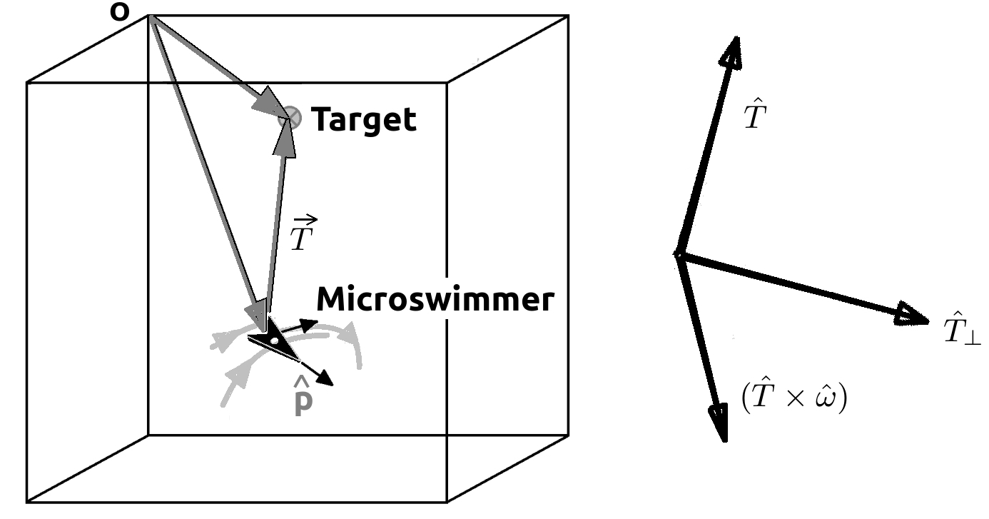
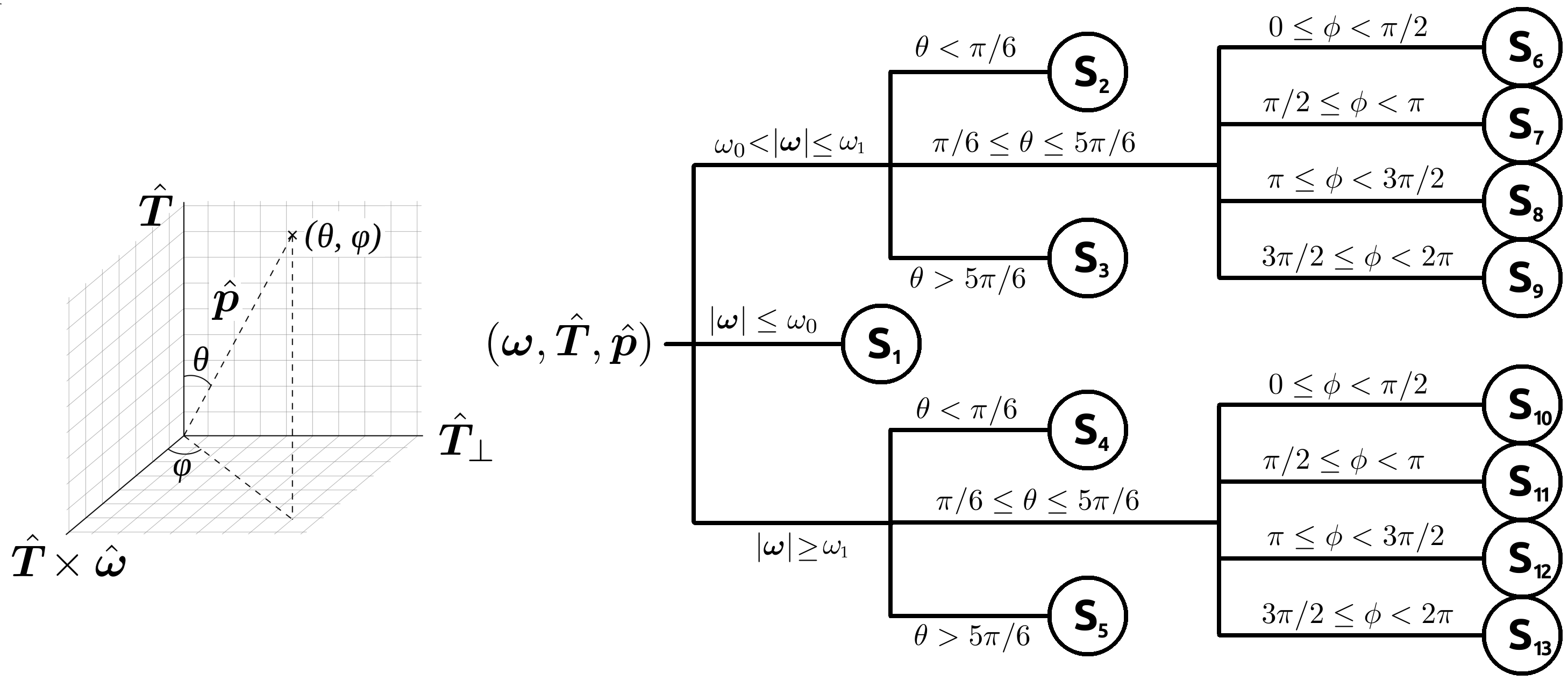
From our DNS of the 3D Navier-Stokes equation we obtain a statistically steady, homogeneous-isotropic turbulent flow in a periodic domain. We introduce passive microswimmers into this flow. To define the states, we fix a coordinate triad, defined by as shown in fig. 9; here, is the unit vector pointing from the microswimmer to the target, is the vorticity pseudo-vector, and is defined by the conditions and . This coordinate system is ill-defined if is parallel to . To implement our -learning in 3D, we define 13 states: (see fig. 10); and 6 actions, . Consequently, the matrix is an array of size .
