Elastic multipole method for describing linear deformation of
infinite 2D solid structures with circular holes and inclusions

Siddhartha Sarkar Department of Electrical Engineering, Princeton University, Princeton, NJ 08544, USA    Matjaž Čebron Faculty of Mechanical Engineering, University of Ljubljana, SI-1000 Ljubljana, Slovenia    Miha Brojan miha.brojan@fs.uni-lj.si Faculty of Mechanical Engineering, University of Ljubljana, SI-1000 Ljubljana, Slovenia    Andrej Košmrlj andrej@princeton.edu Department of Mechanical and Aerospace Engineering, Princeton University, Princeton, NJ 08544, USA Princeton Institute for the Science and Technology of Materials, Princeton University, Princeton, NJ 08544, USA
Abstract

Elastic materials with holes and inclusions are important in a large variety of contexts ranging from construction material to biological membranes. More recently, they have also been exploited in mechanical metamaterials, where the geometry of highly deformable structures is responsible for their unusual properties, such as negative Poisson’s ratio, mechanical cloaking, and tunable phononic band gaps. Understanding how such structures deform in response to applied external loads is thus crucial for designing novel mechanical metamaterials. Here we present a method for predicting the linear response of infinite 2D solid structures with circular holes and inclusions by employing analogies with electrostatics. Just like an external electric field induces polarization (dipoles, quadrupoles and other multipoles) of conductive and dielectric objects, external stress induces elastic multipoles inside holes and inclusions. Stresses generated by these induced elastic multipoles then lead to interactions between holes and inclusions, which induce additional polarization and thus additional deformation of holes and inclusions. We present a method that expands the induced polarization in a series of elastic multipoles, which systematically takes into account the interactions of inclusions and holes with the external stress field and also between them. The results of our method show good agreement with both linear finite element simulations and experiments.

I Introduction

Elastic materials with holes and inclusions have been studied extensively in materials science. Typically, the goal is to homogenize the microscale distribution of holes and inclusions to obtain effective material properties on the macroscale Eshelby ; Hashin ; Castaneda ; Torquato , where the detailed micropattern of deformations and stresses is ignored. On the other hand, it has recently been recognized that the microscale interactions between proteins embedded in biological membranes can promote the assembly of ordered protein structures ProteinAssembly2 ; ProteinAssembly ; Haselwandter and can also facilitate the entry of virus particles into cells Protein . Furthermore, in mechanical metamaterials bertoldi2017flexible , the geometry, topology and contrasting elastic properties of different materials are exploited to achieve extraordinary functionalities, such as shape morphing ShapeMorph ; ShapeMorph2 , mechanical cloaking Cloaking ; Cloaking2 ; Cloaking3 , negative Poisson’s ratio almgren1985isotropic ; lakes1987foam ; Auxetic2 ; Auxetic ; babaee20133d , negative thermal expansion NegativeThermalExpansion ; NegativeThermalExpansion2 , effective negative swelling NegativeSwelling ; NegativeSwelling2 ; NegativeSwelling3 , and tunable phononic band gaps BandGap3 ; BandGap ; BandGap2 . At the heart of these functionalities are deformation patterns of such materials with holes and inclusions. Therefore, understanding how these structures deform under applied external load is crucial for the design of novel metamaterials.
Refer to caption
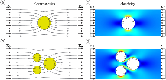
Figure 1: Induction in electrostatics and elasticity. (a,b) Induced polarization due to the external electric field 𝐄0subscript𝐄0\mathbf{E}_{0} of (a) a single and (b) multiple conducting spheres (yellow). The resultant electric field lines are shown in grey color. (c,d) Induced quadrupoles due to external uniaxial compressive stress σ0subscript𝜎0\sigma_{0} in (c) a single and (d) multiple circular holes (white disks) embedded in an elastic matrix. Heat maps show the von Mises stress field, where red and blue colors indicate regions of high and low von Mises stress, respectively.

Linear deformations of infinite thin plates with circular holes under external load have been studied extensively over the years Green ; Haddon ; Ukadgaonker ; Ting ; Hoang08 . The solution for one hole can be easily obtained using standard techniques Barber and the solution for two holes can be constructed with conformal maps and complex analysis Haddon . Green demonstrated how to construct a solution for infinite thin plates with any number of holes Green by expanding the Airy stress function around each hole in terms of the Michell solution for biharmonic functions Michell . However, it remained unclear how this procedure could be generalized to finite structures with boundaries.

Deformations of thin membranes with infinitely rigid inclusions have also received a lot of attention, especially in the context of rigid proteins embedded in biological membranes goulian1993long ; park1996interactions ; golestanian1996fluctuationPRE ; golestanian1996fluctuationEPL ; weikl1998interaction ; ProteinAssembly ; yolcu2012membrane ; Deserno ; Haselwandter ; Protein ; Purohit . Several different approaches were developed to study the elastic and entropic interactions between inclusions, such as multipole expansion goulian1993long , the effective field theory approach yolcu2012membrane ; Deserno , and homogenization Protein . Even though these articles considered membrane bending, the governing equation for the out-of-plane displacement is also biharmonic to the lowest order. Hence these methods could be adapted to investigate the in-plane deformations of plates with rigid inclusions.

In two companion papers, we have generalized Green’s method Green by employing analogies with electrostatics to describe the linear response of a thin elastic plate (plane stress) or an infinitely thick elastic matrix (plane strain) with embedded cylindrical holes and inclusions, which can be treated as a 2D problem with circular holes and inclusions. Just like a polarized conductive object in an external electric field can be described by induced dipole (see Fig. 1a), a hole deformed by the external load can be described by induced elastic quadrupoles (see Fig. 1c). Circular inclusions in the elastic matrix under external load are analogous to dielectric objects in an external electric field. When multiple conductive objects are placed in an external electric field, the induced polarizations generate additional electric fields, which lead to further charge redistribution on the surface of conductive objects (see Fig. 1b). Similarly, induced quadrupoles in deformed holes generate additional stresses in the elastic matrix, which lead to further deformations of holes (see Fig. 1d).

In this paper, we present a method to describe linear deformations of circular holes and inclusions embedded in an infinite 2D elastic matrix under small external loads by systematically expanding induced polarization of each hole/inclusion in terms of elastic multipoles that are related to terms in the Michell solution for biharmonic functions Michell . The results of this method are compared with linear finite element simulations and experiments. We show that the error decreases exponentially as the maximum degree of elastic multipoles is increased. In the companion paper sarkar2020image , we describe how this method can be generalized to finite size structures by employing ideas of image charges, which become important for holes and inclusions near boundaries.

The remaining part of the paper is organized as follows. In Section II, we review the analogy between electrostatics and 2D linear elasticity and introduce important concepts borrowed from electrostatics. In Section III, we describe the method for evaluating linear deformation of structures with holes and inclusions under external load, which is compared with linear finite element simulations and experiments. In Section IV, we give concluding remarks and comment on the extensions of this method to the nonlinear deformation regime, which is also important for the analysis of mechanical metamaterials.

II Analogy between electrostatics and 2D linear elasticity

The analogy between electrostatics and 2D linear elasticity can be recognized, when the governing equations are formulated in terms of the electric potential U𝑈U Jackson and the Airy stress function χ𝜒\chi Barber , respectively, which are summarized in Table 1. The measurable fields, namely the electric field 𝐄𝐄\mathbf{E} and the stress tensor field σijsubscript𝜎𝑖𝑗\sigma_{ij}, are obtained by taking spatial derivatives of these scalar functions, as shown in Eqs. (1) and (1), where ϵijsubscriptitalic-ϵ𝑖𝑗\epsilon_{ij} is the permutation symbol (ϵ12=ϵ21=1,ϵ11=ϵ22=0formulae-sequencesubscriptitalic-ϵ12subscriptitalic-ϵ211subscriptitalic-ϵ11subscriptitalic-ϵ220\epsilon_{12}=-\epsilon_{21}=1,\epsilon_{11}=\epsilon_{22}=0) and summation over repeated indices is implied. The most compelling aspect of the formulations in terms of scalar functions U𝑈U and χ𝜒\chi is that Faraday’s law in electrostatics in Eq. (1) and the force balance in elasticity in Eq. (1) are automatically satisfied. Moreover, the governing equations for these scalar functions take simple forms as shown in Eqs. (1) and (1). Equation (1) describes the well known Gauss’s law, where ρesubscript𝜌𝑒\rho_{e} is the electric charge density and ϵesubscriptitalic-ϵ𝑒\epsilon_{e} is the permittivity of the material. The analogous Eq. (1) in elasticity describes the (in)compatibility conditions Chaikin ; moshe2014plane , where E𝐸E is the 2D Young’s modulus and ρ𝜌\rho is the elastic charge density associated with defects, which are sources of incompatibility. In the absence of electric charges (ρe=0subscript𝜌𝑒0\rho_{e}=0) the electric potential U𝑈U is a harmonic function (see Eq. (1)), while in the absence of defects (ρ=0𝜌0\rho=0) the Airy stress function χ𝜒\chi is a biharmonic function (see Eq. (1)).

Table 1: Comparison between equations in electrostatics and 2D linear elasticity
Electrostatics Elasticity
Scalar potentials U𝑈U χ𝜒\chi
Fields 𝐄=U𝐄bold-∇𝑈\mathbf{E}=-\bm{\nabla}U (1) σij=ϵikϵjl2χxkxlsubscript𝜎𝑖𝑗subscriptitalic-ϵ𝑖𝑘subscriptitalic-ϵ𝑗𝑙superscript2𝜒subscript𝑥𝑘subscript𝑥𝑙\sigma_{ij}=\epsilon_{ik}\epsilon_{jl}\frac{\partial^{2}\chi}{\partial x_{k}\partial x_{l}} (2)
Properties of scalar functions ×𝐄=×U=𝟎bold-∇𝐄bold-∇bold-∇𝑈0\bm{\nabla}\times\mathbf{E}=-\bm{\nabla}\times\bm{\nabla}U=\mathbf{0} (3) σijxj=ϵikϵjlxj2χxkxl=0subscript𝜎𝑖𝑗subscript𝑥𝑗subscriptitalic-ϵ𝑖𝑘subscriptitalic-ϵ𝑗𝑙subscript𝑥𝑗superscript2𝜒subscript𝑥𝑘subscript𝑥𝑙0\frac{\partial\sigma_{ij}}{\partial x_{j}}=\epsilon_{ik}\epsilon_{jl}\frac{\partial}{\partial x_{j}}\frac{\partial^{2}\chi}{\partial x_{k}\partial x_{l}}=0 (4)
Governing equations ΔU=ρe/ϵeΔ𝑈subscript𝜌𝑒subscriptitalic-ϵ𝑒\Delta U=-\rho_{e}/\epsilon_{e} (5) ΔΔχ=EρΔΔ𝜒𝐸𝜌\Delta\Delta\chi=E\rho (6)

When a conductive object is placed in an external electric field, it gets polarized due to the redistribution of charges (see Fig. 1a). This induced polarization generates an additional electric field outside the conductive object, which can be expanded in terms of fictitious multipoles (dipole, quadrupole, and other multipoles) located at the center of the conductive object Jackson . Note that the induced polarization does not include a monopole charge, because the total topological charge is conserved Jackson . Similarly, a hole or inclusion embedded in an elastic matrix gets polarized when the external load is applied (see Fig. 1c). The additional stresses in the elastic matrix due to this induced polarization can again be expanded in terms of fictitious elastic multipoles (quadrupoles and other multipoles) located at the center of hole/inclusion. In elasticity, the induced polarization does not include disclinations (topological monopole) and dislocations (topological dipole), which are topological defects Chaikin . In order to demonstrate this, we first briefly present the multipoles and induction in electrostatics and describe the meaning of their counterparts in elasticity.
Refer to caption
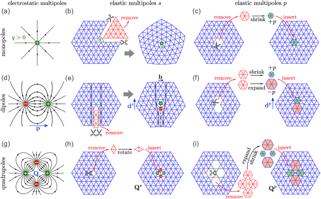
Figure 2: Multipoles in electrostatics and 2D elasticity. (a) An electrostatic monopole with positive charge q𝑞q (green) generates an outward radial electric field (black lines). For a monopole with negative charge, the direction of the electric field is reversed. (b) In 2D elasticity a disclination defect (topological monopole) with charge s𝑠s forms upon removal (s>0𝑠0s>0) or insertion (s<0𝑠0s<0) of a wedge of material (red), where |s|𝑠|s| is the wedge angle. (c) In 2D elasticity, a non-topological monopole p>0𝑝0p>0 (p<0𝑝0p<0) corresponds to a local isotropic contraction (expansion) of the material. (d) An electrostatic dipole 𝐩𝐩\mathbf{p} is formed when a positive (green) and a negative (red) charge of equal magnitude are brought close together. The resulting electric field lines are shown with black lines. (e) In 2D elasticity, a dislocation (topological dipole) forms upon removal or insertion of a semi-infinite strip of material of width |𝐛|𝐛|\mathbf{b}| and is represented by the Burgers vector 𝐛𝐛\mathbf{b}. In a triangular lattice, the dislocation corresponds to two adjacent disclinations of opposite charges. The two black lines indicate the positions of points before and after the removal of a semi-infinite strip (red) from crystal. A dipole moment 𝐝ssuperscript𝐝𝑠\mathbf{d}^{s} can be defined in the direction from negative to positive disclination and its magnitude is equal to the distance between two disclinations times the magnitude of charge of each disclination. (f) In 2D elasticity, a non-topological dipole 𝐝psuperscript𝐝𝑝\mathbf{d}^{p} is formed when a positive (green) and a negative (red) non-topological charge of equal magnitude are brought close together. (g) An electrostatic quadrupole 𝐐𝐐\mathbf{Q} consisting of four charges at the vertices of a square with opposite charges at the adjacent vertices. The resulting electric field lines are shown with black lines. (h) In 2D elasticity, a quadrupole 𝐐ssuperscript𝐐𝑠\mathbf{Q}^{s} is represented by four disclinations at the vertices of a square with opposite charges at the adjacent vertices. Due to the quadrupole 𝐐ssuperscript𝐐𝑠\mathbf{Q}^{s}, material locally expands in the direction of positive disclinations and locally contracts in the direction of negative disclinations, while the total area remains locally unchanged. (i) In 2D elasticity, a quadrupole 𝐐psuperscript𝐐𝑝\mathbf{Q}^{p} is represented by four non-topological monopoles at the vertices of a square with opposite charges at the adjacent vertices.

II.1 Monopoles

In electrostatics, a topological monopole is defined as the electric charge density distribution proportional to the Dirac delta function, i.e. ρe=qδ(𝐱𝐱0)subscript𝜌𝑒𝑞𝛿𝐱subscript𝐱0\rho_{e}=q\delta(\mathbf{x}-\mathbf{x}_{0}), where q𝑞q is the charge and 𝐱0subscript𝐱0\mathbf{x}_{0} denotes its position. The electric potential Um(𝐱𝐱0|q)subscript𝑈𝑚𝐱conditionalsubscript𝐱0𝑞U_{m}(\mathbf{x}-\mathbf{x}_{0}|q) in 2D is then obtained by solving the governing equation as Jackson

ΔUm=qϵeδ(𝐱𝐱0)Um(𝐱𝐱0|q)=q2πϵeln|𝐱𝐱0|.formulae-sequenceΔsubscript𝑈𝑚𝑞subscriptitalic-ϵ𝑒𝛿𝐱subscript𝐱0subscript𝑈𝑚𝐱conditionalsubscript𝐱0𝑞𝑞2𝜋subscriptitalic-ϵ𝑒𝐱subscript𝐱0\Delta U_{m}=-\frac{q}{\epsilon_{e}}\delta(\mathbf{x}-\mathbf{x}_{0})\quad\Longrightarrow\quad U_{m}(\mathbf{x}-\mathbf{x}_{0}|q)=-\frac{q}{2\pi\epsilon_{e}}\ln|\mathbf{x}-\mathbf{x}_{0}|. (7)

For the positive monopole charge, the electric field 𝐄m=Umsubscript𝐄𝑚bold-∇subscript𝑈𝑚\mathbf{E}_{m}=-\bm{\nabla}U_{m} is pointing radially outward (see Fig. 2a). Note that the total charge is topologically conserved Jackson .

Similarly, we can define a topological monopole in 2D elasticity as the charge density proportional to the Dirac delta function, i.e. ρ=sδ(𝒙𝒙0)𝜌𝑠𝛿𝒙subscript𝒙0\rho=s\delta(\bm{x}-\bm{x}_{0}), where s𝑠s is the charge and 𝐱0subscript𝐱0\mathbf{x}_{0} denotes its position. Topological monopoles are called disclinations and their Airy stress function χms(𝐱𝐱0|s)superscriptsubscript𝜒𝑚𝑠𝐱conditionalsubscript𝐱0𝑠\chi_{m}^{s}(\mathbf{x}-\mathbf{x}_{0}|s) can be obtained by solving the governing equation as Chaikin ; Moshe2

ΔΔχms=Esδ(𝐱𝐱0)χms(𝐱𝐱0|s)=Es8π|𝐱𝐱0|2(ln|𝐱𝐱0|1/2).formulae-sequenceΔΔsuperscriptsubscript𝜒𝑚𝑠𝐸𝑠𝛿𝐱subscript𝐱0superscriptsubscript𝜒𝑚𝑠𝐱conditionalsubscript𝐱0𝑠𝐸𝑠8𝜋superscript𝐱subscript𝐱02𝐱subscript𝐱012\Delta\Delta\chi_{m}^{s}=Es\delta(\mathbf{x}-\mathbf{x}_{0})\quad\Longrightarrow\quad\chi_{m}^{s}(\mathbf{x}-\mathbf{x}_{0}|s)=\frac{Es}{8\pi}|\mathbf{x}-\mathbf{x}_{0}|^{2}\big{(}\ln|\mathbf{x}-\mathbf{x}_{0}|-1/2\big{)}. (8)

The physical interpretation of topological monopoles in 2D elasticity comes from condensed matter theory. When a wedge with angle s𝑠s is cut out from a 2D elastic material and the newly created boundaries of the remaining material are glued together, a positive disclination defect of charge s𝑠s is formed (see Fig. 2b). The negative disclination with charge s<0𝑠0s<0 corresponds to the insertion of a wedge with angle |s|𝑠|s|. The stresses generated by these operations are described with the Airy stress function in Eq. (8). Chaikin ; Moshe2

Unlike in electrostatics, we can also define a non-topological monopole in 2D elasticity as the charge density proportional to ρ=pΔ0δ(𝒙𝒙0)𝜌𝑝subscriptΔ0𝛿𝒙subscript𝒙0\rho=p\Delta_{0}\delta(\bm{x}-\bm{x}_{0}), where p𝑝p is the charge, 𝐱0subscript𝐱0\mathbf{x}_{0} denotes its position, and Δ0subscriptΔ0\Delta_{0} corresponds to the Laplace operator with respect to 𝐱0subscript𝐱0\mathbf{x}_{0}. The corresponding Airy stress function χmp(𝐱𝐱0|p)superscriptsubscript𝜒𝑚𝑝𝐱conditionalsubscript𝐱0𝑝\chi_{m}^{p}(\mathbf{x}-\mathbf{x}_{0}|p) can be obtained by solving the governing equation as Moshe2

ΔΔχmp=EpΔ0δ(𝐱𝐱0)χmp(𝐱𝐱0|p)=Ep2π(ln(|𝐱𝐱0|)+1/2).formulae-sequenceΔΔsuperscriptsubscript𝜒𝑚𝑝𝐸𝑝subscriptΔ0𝛿𝐱subscript𝐱0superscriptsubscript𝜒𝑚𝑝𝐱conditionalsubscript𝐱0𝑝𝐸𝑝2𝜋𝐱subscript𝐱012\Delta\Delta\chi_{m}^{p}=Ep\Delta_{0}\delta(\mathbf{x}-\mathbf{x}_{0})\quad\Longrightarrow\quad\chi_{m}^{p}(\mathbf{x}-\mathbf{x}_{0}|p)=\frac{Ep}{2\pi}(\ln(|\mathbf{x}-\mathbf{x}_{0}|)+1/2). (9)

Note that the Airy stress functions for the non-topological monopole p𝑝p and for the topological monopole s𝑠s are related via χmp(𝐱𝐱0|p)=Δ0χms(𝐱𝐱0|p)superscriptsubscript𝜒𝑚𝑝𝐱conditionalsubscript𝐱0𝑝subscriptΔ0superscriptsubscript𝜒𝑚𝑠𝐱conditionalsubscript𝐱0𝑝\chi_{m}^{p}(\mathbf{x}-\mathbf{x}_{0}|p)=\Delta_{0}\chi_{m}^{s}(\mathbf{x}-\mathbf{x}_{0}|p). The constant term in Eq. (9) does not generate any stresses and can thus be omitted. A positive (negative) non-topological monopole with charge p>0𝑝0p>0 (p<0𝑝0p<0) is related to a local isotropic contraction (expansion) of the material (see Fig 2c). Moshe1 ; Moshe2

II.2 Dipoles

An electrostatic dipole is formed at 𝐱0subscript𝐱0\mathbf{x}_{0} when two opposite charges ±qplus-or-minus𝑞\pm q are located at 𝐱±=𝐱0±𝐚/2subscript𝐱plus-or-minusplus-or-minussubscript𝐱0𝐚2\mathbf{x}_{\pm}=\mathbf{x}_{0}\pm\mathbf{a}/2 (see Fig. 2d). The electric potential for a dipole in 2D is thus

Ud(𝐱𝐱0|𝐩)=Um(𝐱𝐱+|q)+Um(𝐱𝐱|q)\xlongrightarrow|𝐚|0𝐩(𝐱𝐱𝟎)2πϵe|𝐱𝐱0|2,subscript𝑈𝑑𝐱conditionalsubscript𝐱0𝐩subscript𝑈𝑚𝐱conditionalsubscript𝐱𝑞subscript𝑈𝑚𝐱conditionalsubscript𝐱𝑞\xlongrightarrow𝐚0𝐩𝐱subscript𝐱02𝜋subscriptitalic-ϵ𝑒superscript𝐱subscript𝐱02U_{d}(\mathbf{x}-\mathbf{x}_{0}|\mathbf{p})=U_{m}(\mathbf{x}-\mathbf{x}_{+}|q)+U_{m}(\mathbf{x}-\mathbf{x}_{-}|-q)\ \xlongrightarrow{{|\mathbf{a}|\to 0}}\ \frac{\mathbf{p}\cdot(\mathbf{x}-\mathbf{x_{0}})}{2\pi\epsilon_{e}|\mathbf{x}-\mathbf{x}_{0}|^{2}}, (10)

where we introduced the dipole moment 𝐩=q𝐚𝐩𝑞𝐚\mathbf{p}=q\mathbf{a}Jackson Note that in electrostatics dipoles and all higher-order multipoles are non-topological Jackson .

Similarly, a dipole 𝐝s=s𝐚superscript𝐝𝑠𝑠𝐚\mathbf{d}^{s}=s\mathbf{a} in 2D elasticity is formed when two disclination defects of opposite charges ±splus-or-minus𝑠\pm s are located at 𝐱±=𝐱0±𝐚/2subscript𝐱plus-or-minusplus-or-minussubscript𝐱0𝐚2\mathbf{x}_{\pm}=\mathbf{x}_{0}\pm\mathbf{a}/2 (see Fig. 2e). Dipoles are called dislocations and their Airy stress function is Chaikin

χds(𝐱𝐱0|𝐝s)=χms(𝐱𝐱+|s)+χms(𝐱𝐱|s)\xlongrightarrow|𝐚|0E4π𝐝𝐬(𝐱𝐱0)ln|𝐱𝐱0|.subscriptsuperscript𝜒𝑠𝑑𝐱conditionalsubscript𝐱0superscript𝐝𝑠superscriptsubscript𝜒𝑚𝑠𝐱conditionalsubscript𝐱𝑠superscriptsubscript𝜒𝑚𝑠𝐱conditionalsubscript𝐱𝑠\xlongrightarrow𝐚0𝐸4𝜋superscript𝐝𝐬𝐱subscript𝐱0𝐱subscript𝐱0\chi^{s}_{d}(\mathbf{x}-\mathbf{x}_{0}|\mathbf{d}^{s})=\chi_{m}^{s}(\mathbf{x}-\mathbf{x}_{+}|s)+\chi_{m}^{s}(\mathbf{x}-\mathbf{x}_{-}|-s)\ \xlongrightarrow{{|\mathbf{a}|\to 0}}\ -\frac{E}{4\pi}\mathbf{d^{s}}\cdot(\mathbf{x}-\mathbf{x}_{0})\ln|\mathbf{x}-\mathbf{x}_{0}|. (11)

Dislocation is a topological defect, which forms upon removal or insertion of a semi-infinite strip of material of width |𝐛|𝐛|\mathbf{b}| (see Fig. 2e). Note that dislocations are conventionally represented by the Burgers vector 𝐛𝐛\mathbf{b}, which is equal to the dipole moment 𝐝ssuperscript𝐝𝑠\mathbf{d}^{s} rotated by 90, i.e. bi=ϵijdjssubscript𝑏𝑖subscriptitalic-ϵ𝑖𝑗superscriptsubscript𝑑𝑗𝑠b_{i}=\epsilon_{ij}d_{j}^{s}Chaikin ; Moshe2

In 2D elasticity, we can define another non-topological dipole 𝐝p=p𝐚superscript𝐝𝑝𝑝𝐚\mathbf{d}^{p}=p\mathbf{a}, which is formed when two non-topological monopoles of opposite charges ±pplus-or-minus𝑝\pm p are located at 𝐱±=𝐱0±𝐚/2subscript𝐱plus-or-minusplus-or-minussubscript𝐱0𝐚2\mathbf{x}_{\pm}=\mathbf{x}_{0}\pm\mathbf{a}/2 (see Fig. 2f). Their Airy stress function is

χdp(𝐱𝐱0|𝐝p)=χmp(𝐱𝐱+|p)+χmp(𝐱𝐱|p)\xlongrightarrow|𝐚|0E2π𝐝p(𝐱𝐱0)|𝐱𝐱0|2.subscriptsuperscript𝜒𝑝𝑑𝐱conditionalsubscript𝐱0superscript𝐝𝑝superscriptsubscript𝜒𝑚𝑝𝐱conditionalsubscript𝐱𝑝superscriptsubscript𝜒𝑚𝑝𝐱conditionalsubscript𝐱𝑝\xlongrightarrow𝐚0𝐸2𝜋superscript𝐝𝑝𝐱subscript𝐱0superscript𝐱subscript𝐱02\chi^{p}_{d}(\mathbf{x}-\mathbf{x}_{0}|\mathbf{d}^{p})=\chi_{m}^{p}(\mathbf{x}-\mathbf{x}_{+}|p)+\chi_{m}^{p}(\mathbf{x}-\mathbf{x}_{-}|-p)\ \xlongrightarrow{{|\mathbf{a}|\to 0}}\ -\frac{E}{2\pi}\frac{\mathbf{d}^{p}\cdot(\mathbf{x}-\mathbf{x}_{0})}{|\mathbf{x}-\mathbf{x}_{0}|^{2}}. (12)

II.3 Quadrupoles

An electrostatic quadrupole 𝐐𝐐\mathbf{Q} in 2D is formed when two positive and negative charges are placed symmetrically around 𝐱0subscript𝐱0\mathbf{x}_{0}, such that charges qi=q(1)isubscript𝑞𝑖𝑞superscript1𝑖q_{i}=q(-1)^{i} are placed at positions 𝐱i=𝐱0+a(cos(θ+iπ/2),sin(θ+iπ/2))subscript𝐱𝑖subscript𝐱0𝑎𝜃𝑖𝜋2𝜃𝑖𝜋2\mathbf{x}_{i}=\mathbf{x}_{0}+a\big{(}\cos(\theta+i\pi/2),\sin(\theta+i\pi/2)\big{)}, where i{0,1,2,3}𝑖0123i\in\{0,1,2,3\} and angle θ𝜃\theta describes the orientation of quadrupole (see Fig. 2g). The electric potential of the quadrupole is thus

UQ(r,φ|Q,θ)=i=03Um(𝐱𝐱i|qi)\xlongrightarrowa0Qcos(2(φθ))πϵer2,subscript𝑈𝑄𝑟conditional𝜑𝑄𝜃superscriptsubscript𝑖03subscript𝑈𝑚𝐱conditionalsubscript𝐱𝑖subscript𝑞𝑖\xlongrightarrow𝑎0𝑄2𝜑𝜃𝜋subscriptitalic-ϵ𝑒superscript𝑟2U_{Q}(r,\varphi|Q,\theta)=\sum_{i=0}^{3}U_{m}(\mathbf{x}-\mathbf{x}_{i}|q_{i})\ \xlongrightarrow{{a\to 0}}\ \frac{Q\cos\big{(}2(\varphi-\theta)\big{)}}{\pi\epsilon_{e}r^{2}}, (13)

where we introduced the quadrupole moment Q=qa2𝑄𝑞superscript𝑎2Q=qa^{2} and polar coordinates (r=(xx0)2+(yy0)2𝑟superscript𝑥subscript𝑥02superscript𝑦subscript𝑦02r=\sqrt{(x-x_{0})^{2}+(y-y_{0})^{2}}, φ=arctan[(yy0)/(xx0)]𝜑𝑦subscript𝑦0𝑥subscript𝑥0\varphi=\arctan[(y-y_{0})/(x-x_{0})]) centered at 𝐱0subscript𝐱0\mathbf{x}_{0}.

Similarly, an elastic quadrupole 𝐐ssuperscript𝐐𝑠\mathbf{Q}^{s} is formed when two positive and negative disclinations are placed symmetrically around 𝐱0subscript𝐱0\mathbf{x}_{0}, such that disclinations with charges si=s(1)isubscript𝑠𝑖𝑠superscript1𝑖s_{i}=s(-1)^{i} are placed at positions 𝐱i=𝐱0+a(cos(θ+iπ/2),sin(θ+iπ/2))subscript𝐱𝑖subscript𝐱0𝑎𝜃𝑖𝜋2𝜃𝑖𝜋2\mathbf{x}_{i}=\mathbf{x}_{0}+a\big{(}\cos(\theta+i\pi/2),\sin(\theta+i\pi/2)\big{)}, where i{0,1,2,3}𝑖0123i\in\{0,1,2,3\} and angle θ𝜃\theta describes the orientation of quadrupole (see Fig. 2h). The Airy stress function for quadrupole 𝐐ssuperscript𝐐𝑠\mathbf{Q}^{s} in polar coordinates is thus

χQs(r,φ|Qs,θ)=i=03χms(𝐱𝐱i|si)\xlongrightarrowa0EQscos(2(φθ))4π,superscriptsubscript𝜒𝑄𝑠𝑟conditional𝜑superscript𝑄𝑠𝜃superscriptsubscript𝑖03superscriptsubscript𝜒𝑚𝑠𝐱conditionalsubscript𝐱𝑖subscript𝑠𝑖\xlongrightarrow𝑎0𝐸superscript𝑄𝑠2𝜑𝜃4𝜋\chi_{Q}^{s}(r,\varphi|Q^{s},\theta)=\sum_{i=0}^{3}\chi_{m}^{s}(\mathbf{x}-\mathbf{x}_{i}|s_{i})\ \xlongrightarrow{{a\to 0}}\ \frac{EQ^{s}\cos\big{(}2(\varphi-\theta)\big{)}}{4\pi}, (14)

where we introduced the quadrupole moment Qs=sa2superscript𝑄𝑠𝑠superscript𝑎2Q^{s}=sa^{2}. The elastic quadrupole 𝐐ssuperscript𝐐𝑠\mathbf{Q}^{s} causes the material to locally expand in the θ𝜃\theta direction and locally contract in the orthogonal direction (see Fig. 2h). Note that the quadrupole 𝐐ssuperscript𝐐𝑠\mathbf{Q}^{s} is non-topological Moshe1 ; Moshe2 .

In elasticity, we can define another quadrupole 𝐐psuperscript𝐐𝑝\mathbf{Q}^{p}, which is formed when two positive and negative non-topological monopoles are placed symmetrically around 𝐱0subscript𝐱0\mathbf{x}_{0}, such that non-topological charges pi=p(1)isubscript𝑝𝑖𝑝superscript1𝑖p_{i}=p(-1)^{i} are placed at positions 𝐱i=𝐱0+a(cos(θ+iπ/2),sin(θ+iπ/2))subscript𝐱𝑖subscript𝐱0𝑎𝜃𝑖𝜋2𝜃𝑖𝜋2\mathbf{x}_{i}=\mathbf{x}_{0}+a\big{(}\cos(\theta+i\pi/2),\sin(\theta+i\pi/2)\big{)}, where i{0,1,2,3}𝑖0123i\in\{0,1,2,3\} and angle θ𝜃\theta describes the orientation of quadrupole (see Fig. 2i). The Airy stress function for quadrupole 𝐐psuperscript𝐐𝑝\mathbf{Q}^{p} in polar coordinates is thus

χQp(r,φ|Qp,θ)=i=03χmp(𝐱𝐱i|pi)\xlongrightarrowa0EQpcos(2(φθ))πr2,superscriptsubscript𝜒𝑄𝑝𝑟conditional𝜑superscript𝑄𝑝𝜃superscriptsubscript𝑖03superscriptsubscript𝜒𝑚𝑝𝐱conditionalsubscript𝐱𝑖subscript𝑝𝑖\xlongrightarrow𝑎0𝐸superscript𝑄𝑝2𝜑𝜃𝜋superscript𝑟2\chi_{Q}^{p}(r,\varphi|Q^{p},\theta)=\sum_{i=0}^{3}\chi_{m}^{p}(\mathbf{x}-\mathbf{x}_{i}|p_{i})\ \xlongrightarrow{{a\to 0}}\ \frac{EQ^{p}\cos\big{(}2(\varphi-\theta)\big{)}}{\pi r^{2}}, (15)

where we introduced the quadrupole moment Qp=pa2superscript𝑄𝑝𝑝superscript𝑎2Q^{p}=pa^{2}.

II.4 Higher-order multipoles

The procedure described in the previous sections can be generalized to define higher-order multipoles 𝐐nssubscriptsuperscript𝐐𝑠𝑛\mathbf{Q}^{s}_{n} and 𝐐npsubscriptsuperscript𝐐𝑝𝑛\mathbf{Q}^{p}_{n}. In 2D the quadrupole 𝐐ssuperscript𝐐𝑠\mathbf{Q}^{s} is generalized by placing n𝑛n positive and n𝑛n negative disclinations symmetrically around 𝐱0subscript𝐱0\mathbf{x}_{0}, such that disclinations of charges si=s(1)isubscript𝑠𝑖𝑠superscript1𝑖s_{i}=s(-1)^{i} are placed at positions 𝐱i=𝐱0+a(cos(θ+iπ/n),sin(θ+iπ/n))subscript𝐱𝑖subscript𝐱0𝑎𝜃𝑖𝜋𝑛𝜃𝑖𝜋𝑛\mathbf{x}_{i}=\mathbf{x}_{0}+a\big{(}\cos(\theta+i\pi/n),\sin(\theta+i\pi/n)\big{)}, where i{0,1,,2n1}𝑖012𝑛1i~{}\in~{}\{0,1,\ldots,2n-1\} and angle θ𝜃\theta describes the orientation of multipole. The Airy stress functions for such multipoles 𝐐nssubscriptsuperscript𝐐𝑠𝑛\mathbf{Q}^{s}_{n} in polar coordinates are

χns(r,φ|Qns,θ)=i=02n1χms(𝐱𝐱i|si)\xlongrightarrowa0EQnscos(n(φθ))4(n1)πrn2,superscriptsubscript𝜒𝑛𝑠𝑟conditional𝜑superscriptsubscript𝑄𝑛𝑠𝜃superscriptsubscript𝑖02𝑛1superscriptsubscript𝜒𝑚𝑠𝐱conditionalsubscript𝐱𝑖subscript𝑠𝑖\xlongrightarrow𝑎0𝐸superscriptsubscript𝑄𝑛𝑠𝑛𝜑𝜃4𝑛1𝜋superscript𝑟𝑛2\chi_{n}^{s}(r,\varphi|Q_{n}^{s},\theta)=\sum_{i=0}^{2n-1}\chi_{m}^{s}(\mathbf{x}-\mathbf{x}_{i}|s_{i})\ \xlongrightarrow{{a\to 0}}\ \frac{EQ_{n}^{s}\cos\big{(}n(\varphi-\theta)\big{)}}{4(n-1)\pi r^{n-2}}, (16)

where we introduced the multipole moment Qns=sansuperscriptsubscript𝑄𝑛𝑠𝑠superscript𝑎𝑛Q_{n}^{s}=sa^{n}.

The quadrupole 𝐐psuperscript𝐐𝑝\mathbf{Q}^{p} is generalized to higher-order multipoles by placing n𝑛n positive and n𝑛n negative non-topological monopoles symmetrically around 𝐱0subscript𝐱0\mathbf{x}_{0}, such that charges of strength pi=p(1)isubscript𝑝𝑖𝑝superscript1𝑖p_{i}=p(-1)^{i} are placed at positions 𝐱i=𝐱0+a(cos(θ+iπ/n),sin(θ+iπ/n))subscript𝐱𝑖subscript𝐱0𝑎𝜃𝑖𝜋𝑛𝜃𝑖𝜋𝑛\mathbf{x}_{i}=\mathbf{x}_{0}+a\big{(}\cos(\theta+i\pi/n),\sin(\theta+i\pi/n)\big{)}, where i{0,1,,2n1}𝑖012𝑛1i~{}\in~{}\{0,1,\ldots,2n-1\} and angle θ𝜃\theta describes the orientation of multipole. The Airy stress functions for such multipoles 𝐐npsubscriptsuperscript𝐐𝑝𝑛\mathbf{Q}^{p}_{n} in polar coordinates are

χnp(r,φ|Qnp,θ)=i=02n1χmp(𝐱𝐱i|pi)\xlongrightarrowa0EQnpcos(n(φθ))πrn,superscriptsubscript𝜒𝑛𝑝𝑟conditional𝜑superscriptsubscript𝑄𝑛𝑝𝜃superscriptsubscript𝑖02𝑛1superscriptsubscript𝜒𝑚𝑝𝐱conditionalsubscript𝐱𝑖subscript𝑝𝑖\xlongrightarrow𝑎0𝐸superscriptsubscript𝑄𝑛𝑝𝑛𝜑𝜃𝜋superscript𝑟𝑛\chi_{n}^{p}(r,\varphi|Q_{n}^{p},\theta)=\sum_{i=0}^{2n-1}\chi_{m}^{p}(\mathbf{x}-\mathbf{x}_{i}|p_{i})\ \xlongrightarrow{{a\to 0}}\ -\frac{EQ_{n}^{p}\cos\big{(}n(\varphi-\theta)\big{)}}{\pi r^{n}}, (17)

where we introduced the multipole moment Qnp=pansuperscriptsubscript𝑄𝑛𝑝𝑝superscript𝑎𝑛Q_{n}^{p}=pa^{n}.

II.5 Multipoles vs. the Michell solution for biharmonic functions

The elastic multipoles of types s𝑠s and p𝑝p introduced in the previous sections are closely related to the general solution of the biharmonic equation ΔΔχ=0ΔΔ𝜒0\Delta\Delta\chi=0, due to Michell Michell , which is given in polar coordinates (r,φ)𝑟𝜑(r,\varphi) as

χ(r,φ)=A0r2+B0r2lnr+C0lnr+Iφ+(A1r+B1r1+B1rφ+C1r3+D1rlnr)cosφ+(E1r+F1r1+F1rφ+G1r3+H1rlnr)sinφ+n=2(Anrn+Bnrn+Cnrn+2+Dnrn+2)cos(nφ)+n=2(Enrn+Fnrn+Gnrn+2+Hnrn+2)sin(nφ).𝜒𝑟𝜑subscript𝐴0superscript𝑟2subscript𝐵0superscript𝑟2𝑟subscript𝐶0𝑟𝐼𝜑subscript𝐴1𝑟subscript𝐵1superscript𝑟1superscriptsubscript𝐵1𝑟𝜑subscript𝐶1superscript𝑟3subscript𝐷1𝑟𝑟𝜑subscript𝐸1𝑟subscript𝐹1superscript𝑟1superscriptsubscript𝐹1𝑟𝜑subscript𝐺1superscript𝑟3subscript𝐻1𝑟𝑟𝜑superscriptsubscript𝑛2subscript𝐴𝑛superscript𝑟𝑛subscript𝐵𝑛superscript𝑟𝑛subscript𝐶𝑛superscript𝑟𝑛2subscript𝐷𝑛superscript𝑟𝑛2𝑛𝜑superscriptsubscript𝑛2subscript𝐸𝑛superscript𝑟𝑛subscript𝐹𝑛superscript𝑟𝑛subscript𝐺𝑛superscript𝑟𝑛2subscript𝐻𝑛superscript𝑟𝑛2𝑛𝜑\begin{split}\chi(r,\varphi)&=A_{0}r^{2}+B_{0}r^{2}\ln r+C_{0}\ln r+I\varphi\\ &\phantom{=}+(A_{1}r+B_{1}r^{-1}+B_{1}^{\prime}r\varphi+C_{1}r^{3}+D_{1}r\ln r)\cos\varphi\\ &\phantom{=}+(E_{1}r+F_{1}r^{-1}+F_{1}^{\prime}r\varphi+G_{1}r^{3}+H_{1}r\ln r)\sin\varphi\\ &\phantom{=}+\sum_{n=2}^{\infty}(A_{n}r^{n}+B_{n}r^{-n}+C_{n}r^{n+2}+D_{n}r^{-n+2})\cos(n\varphi)\\ &\phantom{=}+\sum_{n=2}^{\infty}(E_{n}r^{n}+F_{n}r^{-n}+G_{n}r^{n+2}+H_{n}r^{-n+2})\sin(n\varphi).\end{split} (18)

The Michell solution above contains the Airy stress functions corresponding to multipoles located at the origin: disclination (r2lnrsuperscript𝑟2𝑟r^{2}\ln r), dislocation (rlnrcosφ𝑟𝑟𝜑r\ln r\cos\varphi, rlnrsinφ𝑟𝑟𝜑r\ln r\sin\varphi), non-topological monopole (lnr𝑟\ln r), non-topological dipole (cosφ/r𝜑𝑟\cos\varphi/r, sinφ/r𝜑𝑟\sin\varphi/r), quadrupole 𝐐ssuperscript𝐐𝑠\mathbf{Q}^{s} (cos(2φ)2𝜑\cos(2\varphi), sin(2φ)2𝜑\sin(2\varphi)), quadrupole 𝐐psuperscript𝐐𝑝\mathbf{Q}^{p} (cos(2φ)/r22𝜑superscript𝑟2\cos(2\varphi)/r^{2}, sin(2φ)/r22𝜑superscript𝑟2\sin(2\varphi)/r^{2}), as well as all higher-order multipoles 𝐐nssubscriptsuperscript𝐐𝑠𝑛\mathbf{Q}^{s}_{n} and 𝐐npsubscriptsuperscript𝐐𝑝𝑛\mathbf{Q}^{p}_{n} (see Eqs. (16, 17)). Note that the Michell solution also contains terms that increase faster than r2superscript𝑟2r^{2} far away from the origin. These terms are associated with stresses that increase away from the origin and can be interpreted as multipoles located at infinity Moshe6 . Due to the connection with elastic multipoles we refer to coefficients Ai,Bi,,Hisubscript𝐴𝑖subscript𝐵𝑖subscript𝐻𝑖A_{i},B_{i},\dots,H_{i} in the Michell solution as the amplitudes of multipoles.

II.6 Induction

As mentioned previously, the external electric field induces polarization in conducting and dielectric objects. Similarly, external stress induces elastic quadrupoles inside holes and inclusions. To make this analogy concrete, we first demonstrate how external electric field in 2D polarizes a single conductive or dielectric disk, and then discuss how external stress induces quadrupoles inside a circular hole or inclusion.

Let us consider a perfectly conductive disk of radius R𝑅R in a uniform external electric field (𝐄=E0𝐱^𝐄subscript𝐸0bold-^𝐱\mathbf{E}=E_{0}\bm{\mathbf{\hat{x}}}) in 2D. This electric field provides a driving force for mobile charges on the disk, which are redistributed until the resulting tangential component of the total electric field at the circumference of the disk is zero. This means that the electric potential is constant on the circumference (r=R𝑟𝑅r=R). Assuming that the electric potential is zero on the circumference of the disk and that the resultant electric field approaches the background field far away from the disk, we can solve the governing Eq. (1) with ρe=0subscript𝜌𝑒0\rho_{e}=0 in polar coordinates to find that the electric potential is Uintot(r,φ)=0superscriptsubscript𝑈intot𝑟𝜑0U_{\text{in}}^{\text{tot}}(r,\varphi)=0 inside the conductive disk (r<R𝑟𝑅r<R) and that the electric potential Uouttot(r,φ)superscriptsubscript𝑈outtot𝑟𝜑U_{\text{out}}^{\text{tot}}(r,\varphi) outside the conductive disk (r>R𝑟𝑅r>R) is given by Smythe

Uouttot(r,φ)=E0rcosφ+E0R2rcosφ,superscriptsubscript𝑈outtot𝑟𝜑subscript𝐸0𝑟𝜑subscript𝐸0superscript𝑅2𝑟𝜑\begin{split}U_{\text{out}}^{\text{tot}}(r,\varphi)&=-E_{0}r\cos\varphi+E_{0}\frac{R^{2}}{r}\cos\varphi,\end{split} (19)

where the origin of the coordinate system is at the center of the conductive disk. The first term in the above Eq. (19) for the electric potential Uouttot(r,φ)superscriptsubscript𝑈outtot𝑟𝜑U_{\text{out}}^{\text{tot}}(r,\varphi) outside the conductive disk is due to the external electric field and the second term can be interpreted as the electric potential of an induced electrostatic dipole at the center of the disk (see Eq. (10) and Fig. 1a). This analysis can be generalized to a dielectric disk with dielectric constant ϵinsubscriptitalic-ϵin\epsilon_{\text{in}} that is embedded in a material with the dielectric constant ϵoutsubscriptitalic-ϵout\epsilon_{\text{out}} in a uniform external electric field (𝐄=E0𝐱^𝐄subscript𝐸0bold-^𝐱\mathbf{E}=E_{0}\bm{\mathbf{\hat{x}}}). The electric potentials inside and outside the disk are then given by Smythe

Uintot(r,φ)superscriptsubscript𝑈intot𝑟𝜑\displaystyle U_{\text{in}}^{\text{tot}}(r,\varphi) =E0rcosφ+E0(ϵinϵout)(ϵin+ϵout)rcosφ,absentsubscript𝐸0𝑟𝜑subscript𝐸0subscriptitalic-ϵinsubscriptitalic-ϵoutsubscriptitalic-ϵinsubscriptitalic-ϵout𝑟𝜑\displaystyle=-E_{0}r\cos\varphi+E_{0}\frac{(\epsilon_{\text{in}}-\epsilon_{\text{out}})}{(\epsilon_{\text{in}}+\epsilon_{\text{out}})}r\cos\varphi, (20a)
Uouttot(r,φ)superscriptsubscript𝑈outtot𝑟𝜑\displaystyle U_{\text{out}}^{\text{tot}}(r,\varphi) =E0rcosφ+E0(ϵinϵout)(ϵin+ϵout)R2rcosφ.absentsubscript𝐸0𝑟𝜑subscript𝐸0subscriptitalic-ϵinsubscriptitalic-ϵoutsubscriptitalic-ϵinsubscriptitalic-ϵoutsuperscript𝑅2𝑟𝜑\displaystyle=-E_{0}r\cos\varphi+E_{0}\frac{(\epsilon_{\text{in}}-\epsilon_{\text{out}})}{(\epsilon_{\text{in}}+\epsilon_{\text{out}})}\frac{R^{2}}{r}\cos\varphi. (20b)

The first terms in both Uintotsuperscriptsubscript𝑈intotU_{\text{in}}^{\text{tot}} and Uouttotsuperscriptsubscript𝑈outtotU_{\text{out}}^{\text{tot}} correspond to the external electric field, whereas the second terms can be interpreted as induced dipoles. The expression in Eq. (19) for the conductive disk is recovered in the limit ϵin/ϵoutsubscriptitalic-ϵinsubscriptitalic-ϵout\epsilon_{\text{in}}/\epsilon_{\text{out}}~{}\rightarrow~{}\infty. Note that the resulting electric field inside the dielectric disk is uniform 𝐄intot=Uintot=2E0ϵout/(ϵin+ϵout)𝐱^subscriptsuperscript𝐄totinbold-∇subscriptsuperscript𝑈totin2subscript𝐸0subscriptitalic-ϵoutsubscriptitalic-ϵinsubscriptitalic-ϵout^𝐱\mathbf{E}^{\text{tot}}_{\text{in}}=-\bm{\nabla}U^{\text{tot}}_{\text{in}}=2E_{0}\epsilon_{\text{out}}/(\epsilon_{\text{in}}+\epsilon_{\text{out}})\mathbf{\hat{x}}.

Similarly, external stress induces multipoles in elastic systems. For example, consider a circular hole of radius R𝑅R embedded in an infinite elastic matrix. Under external stress σxxext=σ0subscriptsuperscript𝜎ext𝑥𝑥subscript𝜎0\sigma^{\textrm{ext}}_{xx}=-\sigma_{0}, the resultant Airy stress function is obtained by solving the governing Eq. (1) with ρ=0𝜌0\rho=0 with the traction-free boundary condition (σrr=σrφ=0subscript𝜎𝑟𝑟subscript𝜎𝑟𝜑0\sigma_{rr}=\sigma_{r\varphi}=0) at the circumference of the hole. The Airy stress function outside the hole (r>R𝑟𝑅r>R) in polar coordinates is given by Kamien

χouttot(r,φ)=σ0r24(1cos(2φ))+σ0R22lnrσ0R22cos(2φ)+σ0R44r2cos(2φ).subscriptsuperscript𝜒totout𝑟𝜑subscript𝜎0superscript𝑟2412𝜑subscript𝜎0superscript𝑅22𝑟subscript𝜎0superscript𝑅222𝜑subscript𝜎0superscript𝑅44superscript𝑟22𝜑\chi^{\text{tot}}_{\text{out}}(r,\varphi)=-\frac{\sigma_{0}r^{2}}{4}\big{(}1-\cos(2\varphi)\big{)}\,+\,{\frac{\sigma_{0}R^{2}}{2}\ln r}\,-\,{\frac{\sigma_{0}R^{2}}{2}\cos(2\varphi)}\,+\,{\frac{\sigma_{0}R^{4}}{4r^{2}}\cos(2\varphi)}. (21)

The above equation for the Airy stress function reveals that the external stress induces a non-topological monopole p𝑝p (Eq. (9)), and quadrupoles 𝐐ssuperscript𝐐𝑠\mathbf{Q}^{s} and 𝐐psuperscript𝐐𝑝\mathbf{Q}^{p} (Eqs. (14,15)) at the center of the hole (see Fig. 1c). Note that unlike in electrostatics, dipoles 𝐝ssuperscript𝐝𝑠\mathbf{d}^{s} are not induced in elasticity. This is because isolated disclinations (topological monopoles) and dislocations (topological dipoles) are formed by insertion or removal of material, which makes them topological defects Chaikin . On the other hand, elastic non-topological monopole p𝑝p and quadrupoles 𝐐ssuperscript𝐐𝑠\mathbf{Q}^{s} and 𝐐psuperscript𝐐𝑝\mathbf{Q}^{p} can be obtained by local material rearrangement and can thus be induced by external loads Moshe1 ; Moshe2 .

The above analysis can be generalized to the case with a circular inclusion of radius R𝑅R made from material with the Young’s modulus Einsubscript𝐸inE_{\textrm{in}} and the Poisson’s ratio νinsubscript𝜈in\nu_{\textrm{in}} that is embedded in an infinite elastic matrix made from material with the Young’s modulus Eoutsubscript𝐸outE_{\textrm{out}} and the Poisson’s ratio νoutsubscript𝜈out\nu_{\textrm{out}}. Under uniaxial compressive stress σxxext=σ0subscriptsuperscript𝜎ext𝑥𝑥subscript𝜎0\sigma^{\textrm{ext}}_{xx}=-\sigma_{0}, the Airy stress function corresponding to the external stress is χext=σ0y2/2=σ0r2(1cos(2φ))/4subscript𝜒extsubscript𝜎0superscript𝑦22subscript𝜎0superscript𝑟212𝜑4\chi_{\text{ext}}=-\sigma_{0}y^{2}/2=-\sigma_{0}r^{2}\big{(}1-\cos(2\varphi)\big{)}/4. Since the Airy stress function due to external stress contains both the axisymmetric and the cos(2φ)2𝜑\cos(2\varphi) term, the Airy stress function due to induced multipoles should have the same angular dependence. Furthermore stresses should remain finite at the center of the inclusion (r=0𝑟0r=0) and also far away from the inclusion (r𝑟r\rightarrow\infty). The total Airy stress function χintot(r,φ)subscriptsuperscript𝜒totin𝑟𝜑\chi^{\text{tot}}_{\text{in}}(r,\varphi) inside (r<R𝑟𝑅r<R) and χouttot(r,φ)subscriptsuperscript𝜒totout𝑟𝜑\chi^{\text{tot}}_{\text{out}}(r,\varphi) outside (r>R𝑟𝑅r>R) the inclusion can thus be written in the following form

χintot(r,φ)=subscriptsuperscript𝜒totin𝑟𝜑absent\displaystyle\chi^{\text{tot}}_{\text{in}}(r,\varphi)= σ0r24(1cos(2φ))+c0r2+a2r2cos(2φ)+c2r4R2cos(2φ),subscript𝜎0superscript𝑟2412𝜑subscript𝑐0superscript𝑟2subscript𝑎2superscript𝑟22𝜑subscript𝑐2superscript𝑟4superscript𝑅22𝜑\displaystyle-\frac{\sigma_{0}r^{2}}{4}\big{(}1-\cos(2\varphi)\big{)}+c_{0}r^{2}+a_{2}r^{2}\cos(2\varphi)+c_{2}\frac{r^{4}}{R^{2}}\cos(2\varphi), (22a)
χouttot(r,φ)=subscriptsuperscript𝜒totout𝑟𝜑absent\displaystyle\chi^{\text{tot}}_{\text{out}}(r,\varphi)= σ0r24(1cos(2φ))+A0R2ln(rR)+C2R2cos(2φ)+A2R4r2cos(2φ).subscript𝜎0superscript𝑟2412𝜑subscript𝐴0superscript𝑅2𝑟𝑅subscript𝐶2superscript𝑅22𝜑subscript𝐴2superscript𝑅4superscript𝑟22𝜑\displaystyle-\frac{\sigma_{0}r^{2}}{4}\big{(}1-\cos(2\varphi)\big{)}+A_{0}R^{2}\ln\left(\frac{r}{R}\right)+C_{2}R^{2}\cos(2\varphi)+A_{2}R^{4}{r}^{-2}\cos(2\varphi). (22b)

The last three terms in Eq. (22b) correspond to the induced non-topological monopole p𝑝p and quadrupoles 𝐐ssuperscript𝐐𝑠\mathbf{Q}^{s} and 𝐐psuperscript𝐐𝑝\mathbf{Q}^{p} at the center of the inclusion, similar to induced multipoles at the center of the hole in Eq. (21). The last three terms in Eq. (22a) can also be interpreted as induced multipoles that are located far away from the inclusion. The unknown coefficients are determined from the boundary conditions, which require that tractions (σrrsubscript𝜎𝑟𝑟\sigma_{rr} and σrφsubscript𝜎𝑟𝜑\sigma_{r\varphi}) and displacements (ursubscript𝑢𝑟u_{r} and uφsubscript𝑢𝜑u_{\varphi}) are continuous at the circumference of the inclusion (r=R𝑟𝑅r=R). Stresses corresponding to the Airy stress function χ(r,φ)𝜒𝑟𝜑\chi(r,\varphi) can be calculated as σrr=r1(χ/r)+r2(2χ/φ2)subscript𝜎𝑟𝑟superscript𝑟1𝜒𝑟superscript𝑟2superscript2𝜒superscript𝜑2\sigma_{rr}=r^{-1}(\partial\chi/\partial r)+r^{-2}(\partial^{2}\chi/\partial\varphi^{2}), σφφ=2χ/r2subscript𝜎𝜑𝜑superscript2𝜒superscript𝑟2\sigma_{\varphi\varphi}=\partial^{2}\chi/\partial r^{2}, and σrφ=(r1χ/φ)/rsubscript𝜎𝑟𝜑superscript𝑟1𝜒𝜑𝑟\sigma_{r\varphi}=-\partial(r^{-1}\partial\chi/\partial\varphi)/\partial r. Table 2 summarizes the stresses corresponding to different terms in the Michell solution Barber .

Table 2: Stresses σijsubscript𝜎𝑖𝑗\sigma_{ij} and displacements uisubscript𝑢𝑖u_{i} corresponding to different terms for the Airy stress function χ𝜒\chi in the Michell solution Barber . The value of Kolosov’s constant for plane stress is κ=(3ν)/(1+ν)𝜅3𝜈1𝜈\kappa=(3-\nu)/(1+\nu) and for plane strain is κ=34ν𝜅34𝜈\kappa=3-4\nu. Here, μ𝜇\mu is the shear modulus and ν𝜈\nu is the Poisson’s ratio.
χ𝜒\chi σrrsubscript𝜎𝑟𝑟\sigma_{rr} σrφsubscript𝜎𝑟𝜑\sigma_{r\varphi} σφφsubscript𝜎𝜑𝜑\sigma_{\varphi\varphi} 2μ(uruφ)2𝜇matrixsubscript𝑢𝑟subscript𝑢𝜑2\mu\begin{pmatrix}u_{r}\\ u_{\varphi}\end{pmatrix}
r2superscript𝑟2r^{2} 222 00 222 r(κ10)𝑟matrix𝜅10r\,\begin{pmatrix}\kappa-1\\ 0\end{pmatrix}
lnr𝑟\ln r r2superscript𝑟2r^{-2} 00 -r2superscript𝑟2r^{-2} r1(10)superscript𝑟1matrix10r^{-1}\,\begin{pmatrix}-1\\ 0\end{pmatrix}
rn+2cos(nφ)superscript𝑟𝑛2𝑛𝜑r^{n+2}\cos(n\varphi) (n+1)(n2)rncos(nφ)𝑛1𝑛2superscript𝑟𝑛𝑛𝜑-(n+1)(n-2)r^{n}\cos(n\varphi) n(n+1)rnsin(nφ)𝑛𝑛1superscript𝑟𝑛𝑛𝜑n(n+1)r^{n}\sin(n\varphi) (n+1)(n+2)rncos(nφ)𝑛1𝑛2superscript𝑟𝑛𝑛𝜑(n+1)(n+2)r^{n}\cos(n\varphi) rn+1((κn1)cos(nφ)(κ+n+1)sin(nφ))superscript𝑟𝑛1matrix𝜅𝑛1𝑛𝜑𝜅𝑛1𝑛𝜑r^{n+1}\,\begin{pmatrix}(\kappa-n-1)\cos(n\varphi)\\ (\kappa+n+1)\sin(n\varphi)\end{pmatrix}
rn+2sin(nφ)superscript𝑟𝑛2𝑛𝜑r^{n+2}\sin(n\varphi) (n+1)(n2)rnsin(nφ)𝑛1𝑛2superscript𝑟𝑛𝑛𝜑-(n+1)(n-2)r^{n}\sin(n\varphi) n(n+1)rncos(nφ)𝑛𝑛1superscript𝑟𝑛𝑛𝜑-n(n+1)r^{n}\cos(n\varphi) (n+1)(n+2)rnsin(nφ)𝑛1𝑛2superscript𝑟𝑛𝑛𝜑(n+1)(n+2)r^{n}\sin(n\varphi) rn+1((κn1)sin(nφ)(κ+n+1)cos(nφ))superscript𝑟𝑛1matrix𝜅𝑛1𝑛𝜑𝜅𝑛1𝑛𝜑r^{n+1}\,\begin{pmatrix}(\kappa-n-1)\sin(n\varphi)\\ -(\kappa+n+1)\cos(n\varphi)\end{pmatrix}
rn+2cos(nφ)superscript𝑟𝑛2𝑛𝜑r^{-n+2}\cos(n\varphi) (n+2)(n1)rncos(nφ)𝑛2𝑛1superscript𝑟𝑛𝑛𝜑-(n+2)(n-1)r^{-n}\cos(n\varphi) n(n1)rnsin(nφ)𝑛𝑛1superscript𝑟𝑛𝑛𝜑-n(n-1)r^{-n}\sin(n\varphi) (n1)(n2)rncos(nφ)𝑛1𝑛2superscript𝑟𝑛𝑛𝜑(n-1)(n-2)r^{-n}\cos(n\varphi) rn+1((κ+n1)cos(nφ)(κn+1)sin(nφ))superscript𝑟𝑛1matrix𝜅𝑛1𝑛𝜑𝜅𝑛1𝑛𝜑r^{-n+1}\,\begin{pmatrix}(\kappa+n-1)\cos(n\varphi)\\ -(\kappa-n+1)\sin(n\varphi)\end{pmatrix}
rn+2sin(nφ)superscript𝑟𝑛2𝑛𝜑r^{-n+2}\sin(n\varphi) (n+2)(n1)rnsin(nφ)𝑛2𝑛1superscript𝑟𝑛𝑛𝜑-(n+2)(n-1)r^{-n}\sin(n\varphi) n(n1)rncos(nφ)𝑛𝑛1superscript𝑟𝑛𝑛𝜑n(n-1)r^{-n}\cos(n\varphi) (n1)(n2)rnsin(nφ)𝑛1𝑛2superscript𝑟𝑛𝑛𝜑(n-1)(n-2)r^{-n}\sin(n\varphi) rn+1((κ+n1)sin(nφ)(κn+1)cos(nφ))superscript𝑟𝑛1matrix𝜅𝑛1𝑛𝜑𝜅𝑛1𝑛𝜑r^{-n+1}\,\begin{pmatrix}(\kappa+n-1)\sin(n\varphi)\\ (\kappa-n+1)\cos(n\varphi)\end{pmatrix}
rncos(nφ)superscript𝑟𝑛𝑛𝜑r^{n}\cos(n\varphi) n(n1)rn2cos(nφ)𝑛𝑛1superscript𝑟𝑛2𝑛𝜑-n(n-1)r^{n-2}\cos(n\varphi) n(n1)rn2sin(nφ)𝑛𝑛1superscript𝑟𝑛2𝑛𝜑n(n-1)r^{n-2}\sin(n\varphi) n(n1)rn2cos(nφ)𝑛𝑛1superscript𝑟𝑛2𝑛𝜑n(n-1)r^{n-2}\cos(n\varphi) rn1(ncos(nφ)nsin(nφ))superscript𝑟𝑛1matrix𝑛𝑛𝜑𝑛𝑛𝜑r^{n-1}\,\begin{pmatrix}-n\cos(n\varphi)\\ n\sin(n\varphi)\end{pmatrix}
rnsin(nφ)superscript𝑟𝑛𝑛𝜑r^{n}\sin(n\varphi) n(n1)rn2sin(nφ)𝑛𝑛1superscript𝑟𝑛2𝑛𝜑-n(n-1)r^{n-2}\sin(n\varphi) n(n1)rn2cos(nφ)𝑛𝑛1superscript𝑟𝑛2𝑛𝜑-n(n-1)r^{n-2}\cos(n\varphi) n(n1)rn2sin(nφ)𝑛𝑛1superscript𝑟𝑛2𝑛𝜑n(n-1)r^{n-2}\sin(n\varphi) rn1(nsin(nφ)ncos(nφ))superscript𝑟𝑛1matrix𝑛𝑛𝜑𝑛𝑛𝜑r^{n-1}\begin{pmatrix}-n\sin(n\varphi)\\ -n\cos(n\varphi)\end{pmatrix}
rncos(nφ)superscript𝑟𝑛𝑛𝜑r^{-n}\cos(n\varphi) n(n+1)rn2cos(nφ)𝑛𝑛1superscript𝑟𝑛2𝑛𝜑-n(n+1)r^{-n-2}\cos(n\varphi) n(n+1)rn2sin(nφ)𝑛𝑛1superscript𝑟𝑛2𝑛𝜑-n(n+1)r^{-n-2}\sin(n\varphi) n(n+1)rn2cos(nφ)𝑛𝑛1superscript𝑟𝑛2𝑛𝜑n(n+1)r^{-n-2}\cos(n\varphi) rn1(ncos(nφ)nsin(nφ))superscript𝑟𝑛1matrix𝑛𝑛𝜑𝑛𝑛𝜑r^{-n-1}\,\begin{pmatrix}n\cos(n\varphi)\\ n\sin(n\varphi)\end{pmatrix}
rnsin(nφ)superscript𝑟𝑛𝑛𝜑r^{-n}\sin(n\varphi) n(n+1)rn2sin(nφ)𝑛𝑛1superscript𝑟𝑛2𝑛𝜑-n(n+1)r^{-n-2}\sin(n\varphi) n(n+1)rn2cos(nφ)𝑛𝑛1superscript𝑟𝑛2𝑛𝜑n(n+1)r^{-n-2}\cos(n\varphi) n(n+1)rn2sin(nφ)𝑛𝑛1superscript𝑟𝑛2𝑛𝜑n(n+1)r^{-n-2}\sin(n\varphi) rn1(nsin(nφ)ncos(nφ))superscript𝑟𝑛1matrix𝑛𝑛𝜑𝑛𝑛𝜑r^{-n-1}\,\begin{pmatrix}n\sin(n\varphi)\\ -n\cos(n\varphi)\end{pmatrix}

The boundary conditions for tractions (σrrsubscript𝜎𝑟𝑟\sigma_{rr} and σrφsubscript𝜎𝑟𝜑\sigma_{r\varphi}) at the circumference of the inclusion are thus written as

σ02+2c0(σ02+2a2)cos(2φ)=σ02+A0(σ02+4C2+6A2)cos(2φ),(σ02+2a2+6c2)sin(2φ)=(σ022C26A2)sin(2φ).formulae-sequencesubscript𝜎022subscript𝑐0subscript𝜎022subscript𝑎22𝜑subscript𝜎02subscript𝐴0subscript𝜎024subscript𝐶26subscript𝐴22𝜑subscript𝜎022subscript𝑎26subscript𝑐22𝜑subscript𝜎022subscript𝐶26subscript𝐴22𝜑\begin{split}-\frac{\sigma_{0}}{2}+2c_{0}-\left(\frac{\sigma_{0}}{2}+2a_{2}\right)\cos(2\varphi)=&-\frac{\sigma_{0}}{2}+A_{0}-\left(\frac{\sigma_{0}}{2}+4C_{2}+6A_{2}\right)\cos(2\varphi),\\ \left(\frac{\sigma_{0}}{2}+2a_{2}+6c_{2}\right)\sin(2\varphi)=&\left(\frac{\sigma_{0}}{2}-2C_{2}-6A_{2}\right)\sin(2\varphi).\end{split} (23)

In order to obtain displacements, we first calculate the strains εrr=((κ+1)σrr(3κ)σφφ)/(8μ)subscript𝜀𝑟𝑟𝜅1subscript𝜎𝑟𝑟3𝜅subscript𝜎𝜑𝜑8𝜇\varepsilon_{rr}=\left((\kappa+1)\sigma_{rr}-(3-\kappa)\sigma_{\varphi\varphi}\right)/(8\mu), εrφ=σrφ/(2μ)subscript𝜀𝑟𝜑subscript𝜎𝑟𝜑2𝜇\varepsilon_{r\varphi}=\sigma_{r\varphi}/(2\mu) and εφφ=((κ+1)σφφ(3κ)σrr)/(8μ)subscript𝜀𝜑𝜑𝜅1subscript𝜎𝜑𝜑3𝜅subscript𝜎𝑟𝑟8𝜇\varepsilon_{\varphi\varphi}=\left((\kappa+1)\sigma_{\varphi\varphi}-(3-\kappa)\sigma_{rr}\right)/(8\mu), where μ=E/[2(1+ν)]𝜇𝐸delimited-[]21𝜈\mu=E/[2(1+\nu)] is the shear modulus and we introduced the Kolosov’s constant κ=(3ν)/(1+ν)𝜅3𝜈1𝜈\kappa=(3-\nu)/(1+\nu) for plane stress and κ=34ν𝜅34𝜈\kappa=3-4\nu for plane strain condition Barber . Displacements ursubscript𝑢𝑟u_{r} and uφsubscript𝑢𝜑u_{\varphi} are then obtained by integrating the strains. Table 2 summarizes the displacements corresponding to different terms in the Michell solution Barber . The boundary conditions for displacements (ursubscript𝑢𝑟u_{r} and uφsubscript𝑢𝜑u_{\varphi}) at the circumference of inclusion are thus written as

(σ04+c0)R(κin1)2μin+(σ022a2+c2(κin3))Rcos(2φ)2μin=R2μout(14σ0(κout1)+A0)+(σ02+C2(κout+1)+2A2)Rcos(2φ)2μout,(σ02+2a2+c2(κin+3))Rsin(2φ)2μin=(σ02C2(κout1)+2A2)Rsin(2φ)2μout.formulae-sequencesubscript𝜎04subscript𝑐0𝑅subscript𝜅in12subscript𝜇insubscript𝜎022subscript𝑎2subscript𝑐2subscript𝜅in3𝑅2𝜑2subscript𝜇in𝑅2subscript𝜇out14subscript𝜎0subscript𝜅out1subscript𝐴0subscript𝜎02subscript𝐶2subscript𝜅out12subscript𝐴2𝑅2𝜑2subscript𝜇outsubscript𝜎022subscript𝑎2subscript𝑐2subscript𝜅in3𝑅2𝜑2subscript𝜇insubscript𝜎02subscript𝐶2subscript𝜅out12subscript𝐴2𝑅2𝜑2subscript𝜇out\begin{split}&\left(-\frac{\sigma_{0}}{4}+c_{0}\right)\frac{R(\kappa_{\textrm{in}}-1)}{2\mu_{\textrm{in}}}+\left(-\frac{\sigma_{0}}{2}-2a_{2}+c_{2}(\kappa_{\textrm{in}}-3)\right)\frac{R\cos(2\varphi)}{2\mu_{\textrm{in}}}=\\ &\hskip 85.35826pt-\frac{R}{{2\mu_{\textrm{out}}}}\,\left(\frac{1}{4}\sigma_{0}(\kappa_{\textrm{out}}-1)+A_{0}\right)+\left(-\frac{\sigma_{0}}{2}+C_{2}(\kappa_{\textrm{out}}+1)+2A_{2}\right)\frac{R\cos(2\varphi)}{2\mu_{\textrm{out}}},\\ &\left(\frac{\sigma_{0}}{2}+2a_{2}+c_{2}(\kappa_{\textrm{in}}+3)\right)\frac{R\sin(2\varphi)}{2\mu_{\textrm{in}}}=\left(\frac{\sigma_{0}}{2}-C_{2}(\kappa_{\textrm{out}}-1)+2A_{2}\right)\frac{R\sin(2\varphi)}{2\mu_{\textrm{out}}}.\end{split} (24)

The boundary conditions in Eqs. (23) and (24) have to be satisfied at every point (φ𝜑\varphi) on the circumference of the inclusion. Thus the coefficients of the Fourier components have to match on both sides of these equations, which allows us to rewrite the boundary conditions as a matrix equation

(100200064020062026R2μout00R(κin1)2μin000RμoutR(κout+1)2μout0RμinR(κin3)2μin0RμoutR(κout1)2μout0RμinR(κin+3)2μin)(A0A2C2c0a2c2)=(000σ0R8((κout1)μout(κin1)μin)σ0R4(1μout1μin)σ0R4(1μout+1μin)).matrix100200064020062026𝑅2subscript𝜇out00𝑅subscript𝜅in12subscript𝜇in000𝑅subscript𝜇out𝑅subscript𝜅out12subscript𝜇out0𝑅subscript𝜇in𝑅subscript𝜅in32subscript𝜇in0𝑅subscript𝜇out𝑅subscript𝜅out12subscript𝜇out0𝑅subscript𝜇in𝑅subscript𝜅in32subscript𝜇inmatrixsubscript𝐴0subscript𝐴2subscript𝐶2subscript𝑐0subscript𝑎2subscript𝑐2matrix000subscript𝜎0𝑅8subscript𝜅out1subscript𝜇outsubscript𝜅in1subscript𝜇insubscript𝜎0𝑅41subscript𝜇out1subscript𝜇insubscript𝜎0𝑅41subscript𝜇out1subscript𝜇in\begin{pmatrix}1&0&0&-2&0&0\\ 0&-6&-4&0&2&0\\ 0&-6&-2&0&-2&-6\\ -\frac{R}{2\mu_{\textrm{out}}}&0&0&-\frac{R(\kappa_{\textrm{in}}-1)}{2\mu_{\textrm{in}}}&0&0\\ 0&\frac{R}{\mu_{\textrm{out}}}&\frac{R(\kappa_{\textrm{out}}+1)}{2\mu_{\textrm{out}}}&0&\frac{R}{\mu_{\textrm{in}}}&-\frac{R(\kappa_{\textrm{in}}-3)}{2\mu_{\textrm{in}}}\\ 0&\frac{R}{\mu_{\textrm{out}}}&-\frac{R(\kappa_{\textrm{out}}-1)}{2\mu_{\textrm{out}}}&0&-\frac{R}{\mu_{\textrm{in}}}&-\frac{R(\kappa_{\textrm{in}}+3)}{2\mu_{\textrm{in}}}\end{pmatrix}\begin{pmatrix}A_{0}\\ A_{2}\\ C_{2}\\ c_{0}\\ a_{2}\\ c_{2}\end{pmatrix}=\begin{pmatrix}0\\ 0\\ 0\\ \frac{\sigma_{0}R}{8}\left(\frac{(\kappa_{\textrm{out}}-1)}{\mu_{\textrm{out}}}-\frac{(\kappa_{\textrm{in}}-1)}{\mu_{\textrm{in}}}\right)\\ \frac{\sigma_{0}R}{4}\left(\frac{1}{\mu_{\textrm{out}}}-\frac{1}{\mu_{\textrm{in}}}\right)\\ \frac{\sigma_{0}R}{4}\left(-\frac{1}{\mu_{\textrm{out}}}+\frac{1}{\mu_{\textrm{in}}}\right)\end{pmatrix}. (25)

By solving the above set of equations we find that the Airy stress functions χintot(r,φ)subscriptsuperscript𝜒totin𝑟𝜑\chi^{\text{tot}}_{\text{in}}(r,\varphi) inside (r<R𝑟𝑅r<R) and χouttot(r,φ)subscriptsuperscript𝜒totout𝑟𝜑\chi^{\text{tot}}_{\text{out}}(r,\varphi) outside (r>R𝑟𝑅r>R) the inclusion are given by

χintot(r,φ)=subscriptsuperscript𝜒totin𝑟𝜑absent\displaystyle\chi^{\text{tot}}_{\text{in}}(r,\varphi)= σ0r24(1cos(2φ))+(μout(κin1)μin(κout1))4(μout(κin1)+2μin)σ0r2(μoutμin)4(μout+μinκout)σ0r2cos(2φ),subscript𝜎0superscript𝑟2412𝜑subscript𝜇outsubscript𝜅in1subscript𝜇insubscript𝜅out14subscript𝜇outsubscript𝜅in12subscript𝜇insubscript𝜎0superscript𝑟2subscript𝜇outsubscript𝜇in4subscript𝜇outsubscript𝜇insubscript𝜅outsubscript𝜎0superscript𝑟22𝜑\displaystyle-\frac{\sigma_{0}r^{2}}{4}\big{(}1-\cos(2\varphi)\big{)}+\frac{(\mu_{\text{out}}(\kappa_{\text{in}}-1)-\mu_{\text{in}}(\kappa_{\text{out}}-1))}{4(\mu_{\text{out}}(\kappa_{\text{in}}-1)+2\mu_{\text{in}})}\,\sigma_{0}r^{2}-\frac{(\mu_{\text{out}}-\mu_{\text{in}})}{4(\mu_{\text{out}}+\mu_{\text{in}}\kappa_{\text{out}})}\,\sigma_{0}r^{2}\cos(2\varphi), (26a)
χouttot(r,φ)=superscriptsubscript𝜒outtot𝑟𝜑absent\displaystyle\chi_{\text{out}}^{\text{tot}}(r,\varphi)= σ0r24(1cos(2φ))+(μout(κin1)μin(κout1))2(μout(κin1)+2μin)σ0R2lnr(μoutμin)2(μout+μinκout)σ0R2cos(2φ)subscript𝜎0superscript𝑟2412𝜑subscript𝜇outsubscript𝜅in1subscript𝜇insubscript𝜅out12subscript𝜇outsubscript𝜅in12subscript𝜇insubscript𝜎0superscript𝑅2𝑟subscript𝜇outsubscript𝜇in2subscript𝜇outsubscript𝜇insubscript𝜅outsubscript𝜎0superscript𝑅22𝜑\displaystyle-\frac{\sigma_{0}r^{2}}{4}\big{(}1-\cos(2\varphi)\big{)}+\frac{(\mu_{\text{out}}(\kappa_{\text{in}}-1)-\mu_{\text{in}}(\kappa_{\text{out}}-1))}{2(\mu_{\text{out}}(\kappa_{\text{in}}-1)+2\mu_{\text{in}})}\,\sigma_{0}R^{2}\ln r-\frac{(\mu_{\text{out}}-\mu_{\text{in}})}{2(\mu_{\text{out}}+\mu_{\text{in}}\kappa_{\text{out}})}\,\sigma_{0}R^{2}\cos(2\varphi)
+(μoutμin)4(μout+μinκout)σ0R4r2cos(2φ).subscript𝜇outsubscript𝜇in4subscript𝜇outsubscript𝜇insubscript𝜅outsubscript𝜎0superscript𝑅4superscript𝑟22𝜑\displaystyle+\frac{(\mu_{\text{out}}-\mu_{\text{in}})}{4(\mu_{\text{out}}+\mu_{\text{in}}\kappa_{\text{out}})}\sigma_{0}R^{4}r^{-2}\cos(2\varphi). (26b)

In the above Eq. (26) for the Airy stress functions the last three terms can again be interpreted as induced non-topological monopole p𝑝p and quadrupoles 𝐐ssuperscript𝐐𝑠\mathbf{Q}^{s} and 𝐐psuperscript𝐐𝑝\mathbf{Q}^{p}. The expression in Eq. (21) for the hole is recovered in the limit μin0subscript𝜇in0\mu_{\textrm{in}}\rightarrow 0. Note that similar to the Eshelby inclusions in 3D Eshelby , the stress field inside the inclusion in 2D is uniform and is given by

σxxinsubscriptsuperscript𝜎in𝑥𝑥\displaystyle\sigma^{\textrm{in}}_{xx} =σ0μin(1+κout)(μoutκin+μin(2+κout))2(μout(κin1)+2μin)(μout+μinκout),absentsubscript𝜎0subscript𝜇in1subscript𝜅outsubscript𝜇outsubscript𝜅insubscript𝜇in2subscript𝜅out2subscript𝜇outsubscript𝜅in12subscript𝜇insubscript𝜇outsubscript𝜇insubscript𝜅out\displaystyle=-\sigma_{0}\,\frac{\mu_{\text{in}}(1+\kappa_{\text{out}})(\mu_{\text{out}}\kappa_{\text{in}}+\mu_{\text{in}}(2+\kappa_{\text{out}}))}{2(\mu_{\text{out}}(\kappa_{\text{in}}-1)+2\mu_{\text{in}})(\mu_{\text{out}}+\mu_{\text{in}}\kappa_{\text{out}})}, (27a)
σyyinsubscriptsuperscript𝜎in𝑦𝑦\displaystyle\sigma^{\textrm{in}}_{yy} =σ0μin(1+κout)(μout(κin2)μin(κout2))2(μout(κin1)+2μin)(μout+μinκout),absentsubscript𝜎0subscript𝜇in1subscript𝜅outsubscript𝜇outsubscript𝜅in2subscript𝜇insubscript𝜅out22subscript𝜇outsubscript𝜅in12subscript𝜇insubscript𝜇outsubscript𝜇insubscript𝜅out\displaystyle=\sigma_{0}\,\frac{\mu_{\text{in}}(1+\kappa_{\text{out}})(\mu_{\text{out}}(\kappa_{\text{in}}-2)-\mu_{\text{in}}(\kappa_{\text{out}}-2))}{2(\mu_{\text{out}}(\kappa_{\text{in}}-1)+2\mu_{\text{in}})(\mu_{\text{out}}+\mu_{\text{in}}\kappa_{\text{out}})}, (27b)
σxyinsubscriptsuperscript𝜎in𝑥𝑦\displaystyle\sigma^{\textrm{in}}_{xy} =0.absent0\displaystyle=0. (27c)

By comparing the above analyses in elasticity and electrostatics, we conclude that holes and inclusions in elasticity are analogous to perfect conductors and dielectrics in electrostatics, respectively.

The problem of induction becomes much more involved when multiple dielectric objects are considered in electrostatics or multiple inclusions in elasticity. This is because dielectric objects and inclusions interact with each other via induced electric fields and stress fields, respectively. In the next Section, we describe how such interactions can be systematically taken into account in elasticity, which enabled us to calculate the magnitudes of induced multipoles in the presence of external load.

III Elastic multipole method

Building on the concepts described above, we have developed a method for calculating the linear deformation of circular inclusions and holes embedded in an infinite elastic matrix under external stress. External stress induces elastic multipoles at the centers of inclusions and holes, and their amplitudes are obtained from the boundary conditions between different materials (continuity of tractions and displacements). In the following Section III.1, we describe the method for the general case where circular inclusions can have different sizes and material properties (holes correspond to zero shear modulus). Note that our method applies to the deformation of cylindrical holes and inclusions embedded in thin plates (plane stress) as well as to cylindrical holes and inclusions embedded in an infinitely thick elastic matrix (plane strain) by appropriately setting the values of the Kolosov’s constant. In Section III.2 we compare the results of our method to the finite element simulations and in Section III.3 they are compared to experiments.

III.1 Method

Let us consider a 2D infinite elastic matrix with the Young’s modulus E0subscript𝐸0E_{0} and the Poisson’s ratio ν0subscript𝜈0\nu_{0}. Embedded in the matrix are N𝑁N circular inclusions with radii Risubscript𝑅𝑖R_{i} centered at positions 𝐱i=(xi,yi)subscript𝐱𝑖subscript𝑥𝑖subscript𝑦𝑖\mathbf{x}_{i}=(x_{i},y_{i}) with Young’s moduli Eisubscript𝐸𝑖E_{i} and Poisson’s ratios νisubscript𝜈𝑖\nu_{i}, where i{1,,N}𝑖1𝑁i\in\{1,\ldots,N\}. Holes are described with zero Young’s modulus (Ei=0subscript𝐸𝑖0E_{i}=0). External stress, represented with the Airy stress function

χext(x,y)=12σxxexty2+12σyyextx2σxyextxy,subscript𝜒ext𝑥𝑦12superscriptsubscript𝜎𝑥𝑥extsuperscript𝑦212superscriptsubscript𝜎𝑦𝑦extsuperscript𝑥2superscriptsubscript𝜎𝑥𝑦ext𝑥𝑦\chi_{\textrm{ext}}(x,y)=\frac{1}{2}\sigma_{xx}^{\textrm{ext}}y^{2}+\frac{1}{2}\sigma_{yy}^{\textrm{ext}}x^{2}-\sigma_{xy}^{\textrm{ext}}xy, (28)

induces non-topological monopoles (p𝑝p), non-topological dipoles (𝐝psuperscript𝐝𝑝\mathbf{d}^{p}), quadrupoles (𝐐ssuperscript𝐐𝑠\mathbf{Q}^{s}, 𝐐psuperscript𝐐𝑝\mathbf{Q}^{p}), and higher-order multipoles (𝐐nssubscriptsuperscript𝐐𝑠𝑛\mathbf{Q}^{s}_{n}, 𝐐npsubscriptsuperscript𝐐𝑝𝑛\mathbf{Q}^{p}_{n}) at the centers of inclusions, as was discussed in Section II.6. Thus the Airy stress function outside the ithsuperscript𝑖thi^{\text{th}} inclusion due to the induced multipoles can be expanded as

χout(ri,φi|𝐚i,out)=Ai,0Ri2ln(riRi)+n=1Ri2[Ai,n(riRi)ncos(nφi)+Bi,n(riRi)nsin(nφi)]+n=2Ri2[Ci,n(riRi)n+2cos(nφi)+Di,n(riRi)n+2sin(nφi)],subscript𝜒outsubscript𝑟𝑖conditionalsubscript𝜑𝑖subscript𝐚𝑖outsubscript𝐴𝑖0superscriptsubscript𝑅𝑖2subscript𝑟𝑖subscript𝑅𝑖superscriptsubscript𝑛1superscriptsubscript𝑅𝑖2delimited-[]subscript𝐴𝑖𝑛superscriptsubscript𝑟𝑖subscript𝑅𝑖𝑛𝑛subscript𝜑𝑖subscript𝐵𝑖𝑛superscriptsubscript𝑟𝑖subscript𝑅𝑖𝑛𝑛subscript𝜑𝑖superscriptsubscript𝑛2superscriptsubscript𝑅𝑖2delimited-[]subscript𝐶𝑖𝑛superscriptsubscript𝑟𝑖subscript𝑅𝑖𝑛2𝑛subscript𝜑𝑖subscript𝐷𝑖𝑛superscriptsubscript𝑟𝑖subscript𝑅𝑖𝑛2𝑛subscript𝜑𝑖\begin{split}\chi_{\text{out}}\big{(}r_{i},\varphi_{i}|\mathbf{a}_{i,\text{out}}\big{)}=&A_{i,0}R_{i}^{2}\ln\left(\frac{r_{i}}{R_{i}}\right)+\sum_{n=1}^{\infty}R_{i}^{2}\left[A_{i,n}\left(\frac{r_{i}}{R_{i}}\right)^{-n}\cos(n\varphi_{i})+B_{i,n}\left(\frac{r_{i}}{R_{i}}\right)^{-n}\sin(n\varphi_{i})\right]\\ &\quad\quad\quad\quad\quad\quad\quad+\sum_{n=2}^{\infty}R_{i}^{2}\left[C_{i,n}\left(\frac{r_{i}}{R_{i}}\right)^{-n+2}\cos(n\varphi_{i})+D_{i,n}\left(\frac{r_{i}}{R_{i}}\right)^{-n+2}\sin(n\varphi_{i})\right],\end{split} (29)

where the origin of polar coordinates (ri=(xxi)2+(yyi)2,φi=arctan[(yyi)/(xxi)])formulae-sequencesubscript𝑟𝑖superscript𝑥subscript𝑥𝑖2superscript𝑦subscript𝑦𝑖2subscript𝜑𝑖𝑦subscript𝑦𝑖𝑥subscript𝑥𝑖(r_{i}=\sqrt{(x-x_{i})^{2}+(y-y_{i})^{2}},\varphi_{i}=\arctan[(y-y_{i})/(x-x_{i})]) is at the center 𝐱isubscript𝐱𝑖\mathbf{x}_{i} of the ithsuperscript𝑖thi^{\text{th}} inclusion and 𝐚i,out={Ai,0,Ai,1,,Bi,1,Bi,2,,Ci,2,Ci,3,,Di,2,Di,3,}subscript𝐚𝑖outsubscript𝐴𝑖0subscript𝐴𝑖1subscript𝐵𝑖1subscript𝐵𝑖2subscript𝐶𝑖2subscript𝐶𝑖3subscript𝐷𝑖2subscript𝐷𝑖3\mathbf{a}_{i,\text{out}}=\{A_{i,0},A_{i,1},\dots,B_{i,1},B_{i,2},\dots,C_{i,2},C_{i,3},\dots,D_{i,2},D_{i,3},\dots\} is the set of amplitudes of induced multipoles. The total Airy stress function outside all inclusions can then be written as

χouttot(x,y|𝐚out)=χext(x,y)+i=1Nχout(ri(x,y),φi(x,y)|𝐚i,out),subscriptsuperscript𝜒totout𝑥conditional𝑦subscript𝐚outsubscript𝜒ext𝑥𝑦superscriptsubscript𝑖1𝑁subscript𝜒outsubscript𝑟𝑖𝑥𝑦conditionalsubscript𝜑𝑖𝑥𝑦subscript𝐚𝑖out\chi^{\text{tot}}_{\text{out}}\big{(}x,y|\mathbf{a}_{\text{out}}\big{)}=\chi_{\text{ext}}(x,y)+\sum_{i=1}^{N}\chi_{\text{out}}\big{(}r_{i}(x,y),\varphi_{i}(x,y)|\mathbf{a}_{i,\text{out}}\big{)}, (30)

where the first term is due to external stress and the summation describes contributions due to induced multipoles at the centers of inclusions. The set of amplitudes of induced multipoles for all inclusions is defined as 𝐚out={𝐚1,out,,𝐚N,out}subscript𝐚outsubscript𝐚1,outsubscript𝐚𝑁out\mathbf{a}_{\text{out}}=\{\mathbf{a}_{\text{1,out}},\cdots,\mathbf{a}_{N,\text{out}}\}.

Similarly, we expand the induced Airy stress function inside the ithsuperscript𝑖thi^{\text{th}} inclusion as

χin(ri,φi|𝐚i,in)=n=2Ri2[ai,n(riRi)ncos(nφi)+bi,n(riRi)nsin(nφi)]+ci,0ri2+n=1Ri2[ci,n(riRi)n+2cos(nφi)+di,n(riRi)n+2sin(nφi)],subscript𝜒insubscript𝑟𝑖conditionalsubscript𝜑𝑖subscript𝐚𝑖insuperscriptsubscript𝑛2superscriptsubscript𝑅𝑖2delimited-[]subscript𝑎𝑖𝑛superscriptsubscript𝑟𝑖subscript𝑅𝑖𝑛𝑛subscript𝜑𝑖subscript𝑏𝑖𝑛superscriptsubscript𝑟𝑖subscript𝑅𝑖𝑛𝑛subscript𝜑𝑖subscript𝑐𝑖0superscriptsubscript𝑟𝑖2superscriptsubscript𝑛1superscriptsubscript𝑅𝑖2delimited-[]subscript𝑐𝑖𝑛superscriptsubscript𝑟𝑖subscript𝑅𝑖𝑛2𝑛subscript𝜑𝑖subscript𝑑𝑖𝑛superscriptsubscript𝑟𝑖subscript𝑅𝑖𝑛2𝑛subscript𝜑𝑖\begin{split}\chi_{\text{in}}\big{(}r_{i},\varphi_{i}|\mathbf{a}_{i,\text{in}}\big{)}&=\phantom{+c_{i,0}r_{i}^{2}+}\sum_{n=2}^{\infty}R_{i}^{2}\left[a_{i,n}\left(\frac{r_{i}}{R_{i}}\right)^{n}\cos(n\varphi_{i})+b_{i,n}\left(\frac{r_{i}}{R_{i}}\right)^{n}\sin(n\varphi_{i})\right]\\ &\phantom{=}+c_{i,0}r_{i}^{2}+\sum_{n=1}^{\infty}R_{i}^{2}\left[c_{i,n}\left(\frac{r_{i}}{R_{i}}\right)^{n+2}\cos(n\varphi_{i})+d_{i,n}\left(\frac{r_{i}}{R_{i}}\right)^{n+2}\sin(n\varphi_{i})\right],\end{split} (31)

where we kept only the terms that generate finite stresses at the center of inclusion and omitted constant and linear terms {1,ricosφi,risinφi}1subscript𝑟𝑖subscript𝜑𝑖subscript𝑟𝑖subscript𝜑𝑖\{1,r_{i}\cos\varphi_{i},r_{i}\sin\varphi_{i}\} that correspond to zero stresses. The set of amplitudes of induced multipoles is represented as 𝐚i,in={ai,2,ai,3,,bi,2,bi,3,,ci,0,ci,1,,di,1,di,2,}subscript𝐚𝑖insubscript𝑎𝑖2subscript𝑎𝑖3subscript𝑏𝑖2subscript𝑏𝑖3subscript𝑐𝑖0subscript𝑐𝑖1subscript𝑑𝑖1subscript𝑑𝑖2\mathbf{a}_{i,\text{in}}=\{a_{i,2},a_{i,3},\dots,b_{i,2},b_{i,3},\dots,c_{i,0},c_{i,1},\dots,d_{i,1},d_{i,2},\dots\}. The total Airy stress function inside the ithsuperscript𝑖thi^{\text{th}} inclusion is thus

χintot(x,y|𝐚i,in)=χext(x,y)+χin(ri(x,y),φi(x,y)|𝐚i,in),subscriptsuperscript𝜒totin𝑥conditional𝑦subscript𝐚𝑖insubscript𝜒ext𝑥𝑦subscript𝜒insubscript𝑟𝑖𝑥𝑦conditionalsubscript𝜑𝑖𝑥𝑦subscript𝐚𝑖in\chi^{\text{tot}}_{\text{in}}\big{(}x,y|\mathbf{a}_{i,\text{in}}\big{)}=\chi_{\text{ext}}(x,y)+\chi_{\text{in}}\big{(}r_{i}(x,y),\varphi_{i}(x,y)|\mathbf{a}_{i,\text{in}}\big{)}, (32)

where the first term is due to external stress and the second term is due to induced multipoles.

The amplitudes of induced multipoles 𝐚i,outsubscript𝐚𝑖out\mathbf{a}_{i,\text{out}} and 𝐚i,insubscript𝐚𝑖in\mathbf{a}_{i,\text{in}} are obtained by satisfying the boundary conditions that tractions and displacements are continuous across the circumference of each inclusion

σin,rrtot(ri=Ri,φi|𝐚i,in)superscriptsubscript𝜎in𝑟𝑟totsubscript𝑟𝑖subscript𝑅𝑖conditionalsubscript𝜑𝑖subscript𝐚𝑖in\displaystyle\sigma_{\text{in},rr}^{\text{tot}}\big{(}r_{i}=R_{i},\varphi_{i}|\mathbf{a}_{i,\text{in}}\big{)} =σout,rrtot(ri=Ri,φi|𝐚out),absentsuperscriptsubscript𝜎out𝑟𝑟totsubscript𝑟𝑖subscript𝑅𝑖conditionalsubscript𝜑𝑖subscript𝐚out\displaystyle=\sigma_{\text{out},rr}^{\text{tot}}\big{(}r_{i}=R_{i},\varphi_{i}|\mathbf{a}_{\text{out}}\big{)}, (33a)
σin,rφtot(ri=Ri,φi|𝐚i,in)superscriptsubscript𝜎in𝑟𝜑totsubscript𝑟𝑖subscript𝑅𝑖conditionalsubscript𝜑𝑖subscript𝐚𝑖in\displaystyle\sigma_{\text{in},r\varphi}^{\text{tot}}\big{(}r_{i}=R_{i},\varphi_{i}|\mathbf{a}_{i,\text{in}}\big{)} =σout,rφtot(ri=Ri,φi|𝐚out),absentsuperscriptsubscript𝜎out𝑟𝜑totsubscript𝑟𝑖subscript𝑅𝑖conditionalsubscript𝜑𝑖subscript𝐚out\displaystyle=\sigma_{\text{out},r\varphi}^{\text{tot}}\big{(}r_{i}=R_{i},\varphi_{i}|\mathbf{a}_{\text{out}}\big{)}, (33b)
uin,rtot(ri=Ri,φi|𝐚i,in)superscriptsubscript𝑢in𝑟totsubscript𝑟𝑖subscript𝑅𝑖conditionalsubscript𝜑𝑖subscript𝐚𝑖in\displaystyle u_{\text{in},r}^{\text{tot}}\big{(}r_{i}=R_{i},\varphi_{i}|\mathbf{a}_{i,\text{in}}\big{)} =uout,rtot(ri=Ri,φi|𝐚out),absentsuperscriptsubscript𝑢out𝑟totsubscript𝑟𝑖subscript𝑅𝑖conditionalsubscript𝜑𝑖subscript𝐚out\displaystyle=u_{\text{out},r}^{\text{tot}}\big{(}r_{i}=R_{i},\varphi_{i}|\mathbf{a}_{\text{out}}\big{)}, (33c)
uin,φtot(ri=Ri,φi|𝐚i,in)superscriptsubscript𝑢in𝜑totsubscript𝑟𝑖subscript𝑅𝑖conditionalsubscript𝜑𝑖subscript𝐚𝑖in\displaystyle u_{\text{in},\varphi}^{\text{tot}}\big{(}r_{i}=R_{i},\varphi_{i}|\mathbf{a}_{i,\text{in}}\big{)} =uout,φtot(ri=Ri,φi|𝐚out),absentsuperscriptsubscript𝑢out𝜑totsubscript𝑟𝑖subscript𝑅𝑖conditionalsubscript𝜑𝑖subscript𝐚out\displaystyle=u_{\text{out},\varphi}^{\text{tot}}\big{(}r_{i}=R_{i},\varphi_{i}|\mathbf{a}_{\text{out}}\big{)}, (33d)

where stresses and displacements are obtained from the total Airy stress functions χintot(x,y|𝐚i,in)subscriptsuperscript𝜒totin𝑥conditional𝑦subscript𝐚𝑖in\chi^{\text{tot}}_{\text{in}}\big{(}x,y|\mathbf{a}_{i,\text{in}}\big{)} inside the ithsuperscript𝑖thi^{\text{th}} inclusion (see Eq. (32)) and χouttot(x,y|𝐚out)subscriptsuperscript𝜒totout𝑥conditional𝑦subscript𝐚out\chi^{\text{tot}}_{\text{out}}\big{(}x,y|\mathbf{a}_{\text{out}}\big{)} outside all inclusions (see Eq. (30)). In the boundary conditions for the ithsuperscript𝑖thi^{\text{th}} inclusion in the above Eq. (33), we can easily take into account contributions due to the induced multipoles 𝐚i,insubscript𝐚𝑖in\mathbf{a}_{i,\text{in}} and 𝐚i,outsubscript𝐚𝑖out\mathbf{a}_{i,\text{out}} in this inclusion and due to external stresses σxxextsuperscriptsubscript𝜎𝑥𝑥ext\sigma_{xx}^{\textrm{ext}}, σyyextsuperscriptsubscript𝜎𝑦𝑦ext\sigma_{yy}^{\textrm{ext}}, and σxyextsuperscriptsubscript𝜎𝑥𝑦ext\sigma_{xy}^{\textrm{ext}} after rewriting the corresponding Airy stress function χext(x,y)subscript𝜒ext𝑥𝑦\chi_{\textrm{ext}}(x,y) in Eq. (28) in polar coordinates centered at the ithsuperscript𝑖thi^{\text{th}} inclusion as

χext(ri,φi)=14(σxxext+σyyext)ri214(σxxextσyyext)ri2cos(2φi)12σxyextri2sin(2φi).subscript𝜒extsubscript𝑟𝑖subscript𝜑𝑖14superscriptsubscript𝜎𝑥𝑥extsuperscriptsubscript𝜎𝑦𝑦extsuperscriptsubscript𝑟𝑖214superscriptsubscript𝜎𝑥𝑥extsuperscriptsubscript𝜎𝑦𝑦extsuperscriptsubscript𝑟𝑖22subscript𝜑𝑖12superscriptsubscript𝜎𝑥𝑦extsuperscriptsubscript𝑟𝑖22subscript𝜑𝑖\chi_{\textrm{ext}}(r_{i},\varphi_{i})=\frac{1}{4}(\sigma_{xx}^{\textrm{ext}}+\sigma_{yy}^{\textrm{ext}})r_{i}^{2}-\frac{1}{4}(\sigma_{xx}^{\textrm{ext}}-\sigma_{yy}^{\textrm{ext}})r_{i}^{2}\cos(2\varphi_{i})-\frac{1}{2}\sigma_{xy}^{\textrm{ext}}r_{i}^{2}\sin(2\varphi_{i}). (34)

Contributions to stresses and displacements in the boundary conditions for the ithsuperscript𝑖thi^{\text{th}} inclusion in Eq. (33) due to the Airy stress functions χin(ri,φi|𝐚i,in)subscript𝜒insubscript𝑟𝑖conditionalsubscript𝜑𝑖subscript𝐚𝑖in\chi_{\text{in}}\big{(}r_{i},\varphi_{i}|\mathbf{a}_{i,\text{in}}\big{)}, χout(ri,φi|𝐚i,out)subscript𝜒outsubscript𝑟𝑖conditionalsubscript𝜑𝑖subscript𝐚𝑖out\chi_{\text{out}}\big{(}r_{i},\varphi_{i}|\mathbf{a}_{i,\text{out}}\big{)}, and χext(ri,φi)subscript𝜒extsubscript𝑟𝑖subscript𝜑𝑖\chi_{\textrm{ext}}(r_{i},\varphi_{i}) can be taken into account with the help of Table 2. However, it is not straightforward to consider the contributions due to the induced multipoles 𝐚j,outsubscript𝐚𝑗out\mathbf{a}_{j,\text{out}} for other inclusions (ji𝑗𝑖j\neq i), because the corresponding Airy stress functions χout(rj,φj|𝐚j,out)subscript𝜒outsubscript𝑟𝑗conditionalsubscript𝜑𝑗subscript𝐚𝑗out\chi_{\text{out}}\big{(}r_{j},\varphi_{j}|\mathbf{a}_{j,\text{out}}\big{)} in Eq. (29) are written in the polar coordinates centered at 𝐱jsubscript𝐱𝑗\mathbf{x}_{j}. The polar coordinates (rj,φj)subscript𝑟𝑗subscript𝜑𝑗(r_{j},\varphi_{j}) centered at the jthsuperscript𝑗thj^{\text{th}} inclusion can be expressed in terms of polar coordinates (ri,φi)subscript𝑟𝑖subscript𝜑𝑖(r_{i},\varphi_{i}) centered at the ithsuperscript𝑖thi^{\text{th}} inclusion as

rj(ri,φi)=ri2+aij22riaijcos(φiθij),φj(ri,φi)=π+θijarctan[risin(φiθij)(aijricos(φiθij))],formulae-sequencesubscript𝑟𝑗subscript𝑟𝑖subscript𝜑𝑖superscriptsubscript𝑟𝑖2superscriptsubscript𝑎𝑖𝑗22subscript𝑟𝑖subscript𝑎𝑖𝑗subscript𝜑𝑖subscript𝜃𝑖𝑗subscript𝜑𝑗subscript𝑟𝑖subscript𝜑𝑖𝜋subscript𝜃𝑖𝑗subscript𝑟𝑖subscript𝜑𝑖subscript𝜃𝑖𝑗subscript𝑎𝑖𝑗subscript𝑟𝑖subscript𝜑𝑖subscript𝜃𝑖𝑗\begin{split}r_{j}(r_{i},\varphi_{i})&=\sqrt{r_{i}^{2}+a_{ij}^{2}-2r_{i}a_{ij}\cos(\varphi_{i}-\theta_{ij})},\\ \varphi_{j}(r_{i},\varphi_{i})&=\pi+\theta_{ij}-\arctan\left[\frac{r_{i}\sin(\varphi_{i}-\theta_{ij})}{\big{(}a_{ij}-r_{i}\cos(\varphi_{i}-\theta_{ij})\big{)}}\right],\end{split} (35)

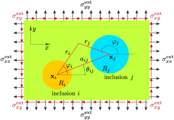
where aij=(xixj)2+(yiyj)2subscript𝑎𝑖𝑗superscriptsubscript𝑥𝑖subscript𝑥𝑗2superscriptsubscript𝑦𝑖subscript𝑦𝑗2a_{ij}=\sqrt{(x_{i}-x_{j})^{2}+(y_{i}-y_{j})^{2}} is the distance between the centers of the ithsuperscript𝑖thi^{\text{th}} and jthsuperscript𝑗thj^{\text{th}} inclusion and θij=arctan[(yjyi)/(xjxi)]subscript𝜃𝑖𝑗subscript𝑦𝑗subscript𝑦𝑖subscript𝑥𝑗subscript𝑥𝑖\theta_{ij}=\arctan[(y_{j}-y_{i})/(x_{j}-x_{i})] is the angle between the line joining the centers of inclusions and the x𝑥x-axis, as shown in Fig. 3.

Refer to caption
Figure 3: Illustration of external load (σxxextsuperscriptsubscript𝜎𝑥𝑥ext\sigma_{xx}^{\text{ext}}, σyyextsuperscriptsubscript𝜎𝑦𝑦ext\sigma_{yy}^{\text{ext}}, σxyextsuperscriptsubscript𝜎𝑥𝑦ext\sigma_{xy}^{\text{ext}}) and polar coordinates (ri,φisubscript𝑟𝑖subscript𝜑𝑖r_{i},\varphi_{i}) and (rj,φjsubscript𝑟𝑗subscript𝜑𝑗r_{j},\varphi_{j}) relative to the centers 𝐱isubscript𝐱𝑖\mathbf{x}_{i} of the ithsuperscript𝑖thi^{\text{th}} inclusion (orange disk) with radius Risubscript𝑅𝑖R_{i} and 𝐱jsubscript𝐱𝑗\mathbf{x}_{j} of the jthsuperscript𝑗thj^{\text{th}} inclusion (blue disk) with radius Rjsubscript𝑅𝑗R_{j}, respectively. Here, aijsubscript𝑎𝑖𝑗a_{ij} is the separation distance between the ithsuperscript𝑖thi^{\text{th}} and jthsuperscript𝑗thj^{\text{th}} inclusion and θijsubscript𝜃𝑖𝑗\theta_{ij} is the angle between the line joining their centers and the x𝑥x-axis.

The Airy stress function due to the induced multipoles centered at the jthsuperscript𝑗thj^{\text{th}} inclusion can be expanded in Taylor series around the center of the ithsuperscript𝑖thi^{\text{th}} inclusion as Green

χout(rj(ri,φi),φj(ri,φi)|𝐚j,out)=n=2Rj2rinaijn[cos(nφi)fcn(Rj/aij,θij|𝐚j,out)+sin(nφi)fsn(Rj/aij,θij|𝐚j,out)]+n=0Rj2rin+2aijn+2[cos(nφi)gcn(Rj/aij,θij|𝐚j,out)+sin(nφi)gsn(Rj/aij,θij|𝐚j,out)],subscript𝜒outsubscript𝑟𝑗subscript𝑟𝑖subscript𝜑𝑖conditionalsubscript𝜑𝑗subscript𝑟𝑖subscript𝜑𝑖subscript𝐚j,outsuperscriptsubscript𝑛2superscriptsubscript𝑅𝑗2superscriptsubscript𝑟𝑖𝑛superscriptsubscript𝑎𝑖𝑗𝑛delimited-[]𝑛subscript𝜑𝑖subscriptsuperscript𝑓𝑛𝑐subscript𝑅𝑗subscript𝑎𝑖𝑗conditionalsubscript𝜃𝑖𝑗subscript𝐚𝑗out𝑛subscript𝜑𝑖subscriptsuperscript𝑓𝑛𝑠subscript𝑅𝑗subscript𝑎𝑖𝑗conditionalsubscript𝜃𝑖𝑗subscript𝐚𝑗outsuperscriptsubscript𝑛0superscriptsubscript𝑅𝑗2superscriptsubscript𝑟𝑖𝑛2superscriptsubscript𝑎𝑖𝑗𝑛2delimited-[]𝑛subscript𝜑𝑖subscriptsuperscript𝑔𝑛𝑐subscript𝑅𝑗subscript𝑎𝑖𝑗conditionalsubscript𝜃𝑖𝑗subscript𝐚𝑗out𝑛subscript𝜑𝑖subscriptsuperscript𝑔𝑛𝑠subscript𝑅𝑗subscript𝑎𝑖𝑗conditionalsubscript𝜃𝑖𝑗subscript𝐚𝑗out\begin{split}\chi_{\text{out}}\big{(}r_{j}(r_{i},\varphi_{i}),\varphi_{j}(r_{i},\varphi_{i})|\mathbf{a}_{\textrm{j,out}}\big{)}=&\quad\sum_{n=2}^{\infty}R_{j}^{2}\frac{r_{i}^{n}}{a_{ij}^{n}}\Big{[}\cos(n\varphi_{i})f^{n}_{c}\left(R_{j}/a_{ij},\theta_{ij}|\mathbf{a}_{j,\textrm{out}}\right)+\sin(n\varphi_{i})f^{n}_{s}\left(R_{j}/a_{ij},\theta_{ij}|\mathbf{a}_{j,\textrm{out}}\right)\Big{]}\\ &+\sum_{n=0}^{\infty}R_{j}^{2}\frac{r_{i}^{n+2}}{a_{ij}^{n+2}}\Big{[}\cos(n\varphi_{i})g^{n}_{c}\left(R_{j}/a_{ij},\theta_{ij}|\mathbf{a}_{j,\textrm{out}}\right)+\sin(n\varphi_{i})g^{n}_{s}\left(R_{j}/a_{ij},\theta_{ij}|\mathbf{a}_{j,\textrm{out}}\right)\Big{]},\end{split} (36)

where we omitted constant and linear terms {1,ricosφi,risinφi}1subscript𝑟𝑖subscript𝜑𝑖subscript𝑟𝑖subscript𝜑𝑖\{1,r_{i}\cos\varphi_{i},r_{i}\sin\varphi_{i}\} that correspond to zero stresses and we introduced functions

fcn(Rj/aij,θij|𝐚j,out)subscriptsuperscript𝑓𝑛𝑐subscript𝑅𝑗subscript𝑎𝑖𝑗conditionalsubscript𝜃𝑖𝑗subscript𝐚𝑗out\displaystyle f^{n}_{c}\left(R_{j}/a_{ij},\theta_{ij}|\mathbf{a}_{j,\textrm{out}}\right) =m=0(Rjmaijm[Aj,m𝒜nm(θij)+Bj,mnm(θij)]+Rjm2aijm2[Cj,m𝒞nm(θij)+Dj,m𝒟nm(θij)]),absentsuperscriptsubscript𝑚0superscriptsubscript𝑅𝑗𝑚superscriptsubscript𝑎𝑖𝑗𝑚delimited-[]subscript𝐴𝑗𝑚superscriptsubscript𝒜𝑛𝑚subscript𝜃𝑖𝑗subscript𝐵𝑗𝑚superscriptsubscript𝑛𝑚subscript𝜃𝑖𝑗superscriptsubscript𝑅𝑗𝑚2superscriptsubscript𝑎𝑖𝑗𝑚2delimited-[]subscript𝐶𝑗𝑚superscriptsubscript𝒞𝑛𝑚subscript𝜃𝑖𝑗subscript𝐷𝑗𝑚superscriptsubscript𝒟𝑛𝑚subscript𝜃𝑖𝑗\displaystyle=\sum_{m=0}^{\infty}\left(\frac{R_{j}^{m}}{a_{ij}^{m}}\Big{[}A_{j,m}\mathcal{A}_{n}^{m}(\theta_{ij})+B_{j,m}\mathcal{B}_{n}^{m}(\theta_{ij})\Big{]}+\frac{R_{j}^{m-2}}{a_{ij}^{m-2}}\Big{[}C_{j,m}\mathcal{C}_{n}^{m}(\theta_{ij})+D_{j,m}\mathcal{D}_{n}^{m}(\theta_{ij})\Big{]}\right), (37a)
fsn(Rj/aij,θij|𝐚j,out)subscriptsuperscript𝑓𝑛𝑠subscript𝑅𝑗subscript𝑎𝑖𝑗conditionalsubscript𝜃𝑖𝑗subscript𝐚𝑗out\displaystyle f^{n}_{s}\left(R_{j}/a_{ij},\theta_{ij}|\mathbf{a}_{j,\textrm{out}}\right) =m=0(Rjmaijm[Aj,mnm(θij)Bj,m𝒜nm(θij)]+Rjm2aijm2[Cj,m𝒟nm(θij)Dj,m𝒞nm(θij)]),absentsuperscriptsubscript𝑚0superscriptsubscript𝑅𝑗𝑚superscriptsubscript𝑎𝑖𝑗𝑚delimited-[]subscript𝐴𝑗𝑚superscriptsubscript𝑛𝑚subscript𝜃𝑖𝑗subscript𝐵𝑗𝑚superscriptsubscript𝒜𝑛𝑚subscript𝜃𝑖𝑗superscriptsubscript𝑅𝑗𝑚2superscriptsubscript𝑎𝑖𝑗𝑚2delimited-[]subscript𝐶𝑗𝑚superscriptsubscript𝒟𝑛𝑚subscript𝜃𝑖𝑗subscript𝐷𝑗𝑚superscriptsubscript𝒞𝑛𝑚subscript𝜃𝑖𝑗\displaystyle=\sum_{m=0}^{\infty}\left(\frac{R_{j}^{m}}{a_{ij}^{m}}\Big{[}A_{j,m}\mathcal{B}_{n}^{m}(\theta_{ij})-B_{j,m}\mathcal{A}_{n}^{m}(\theta_{ij})\Big{]}+\frac{R_{j}^{m-2}}{a_{ij}^{m-2}}\Big{[}C_{j,m}\mathcal{D}_{n}^{m}(\theta_{ij})-D_{j,m}\mathcal{C}_{n}^{m}(\theta_{ij})\Big{]}\right), (37b)
gcn(Rj/aij,θij|𝐚j,out)subscriptsuperscript𝑔𝑛𝑐subscript𝑅𝑗subscript𝑎𝑖𝑗conditionalsubscript𝜃𝑖𝑗subscript𝐚𝑗out\displaystyle g^{n}_{c}\left(R_{j}/a_{ij},\theta_{ij}|\mathbf{a}_{j,\textrm{out}}\right) =m=2Rjm2aijm2[Cj,mnm(θij)+Dj,mnm(θij)],absentsuperscriptsubscript𝑚2superscriptsubscript𝑅𝑗𝑚2superscriptsubscript𝑎𝑖𝑗𝑚2delimited-[]subscript𝐶𝑗𝑚superscriptsubscript𝑛𝑚subscript𝜃𝑖𝑗subscript𝐷𝑗𝑚superscriptsubscript𝑛𝑚subscript𝜃𝑖𝑗\displaystyle=\sum_{m=2}^{\infty}\frac{R_{j}^{m-2}}{a_{ij}^{m-2}}\Big{[}C_{j,m}\mathcal{E}_{n}^{m}(\theta_{ij})+D_{j,m}\mathcal{F}_{n}^{m}(\theta_{ij})\Big{]}, (37c)
gsn(Rj/aij,θij|𝐚j,out)subscriptsuperscript𝑔𝑛𝑠subscript𝑅𝑗subscript𝑎𝑖𝑗conditionalsubscript𝜃𝑖𝑗subscript𝐚𝑗out\displaystyle g^{n}_{s}\left(R_{j}/a_{ij},\theta_{ij}|\mathbf{a}_{j,\textrm{out}}\right) =m=2Rjm2aijm2[Cj,mnm(θij)Dj,mnm(θij)].absentsuperscriptsubscript𝑚2superscriptsubscript𝑅𝑗𝑚2superscriptsubscript𝑎𝑖𝑗𝑚2delimited-[]subscript𝐶𝑗𝑚superscriptsubscript𝑛𝑚subscript𝜃𝑖𝑗subscript𝐷𝑗𝑚superscriptsubscript𝑛𝑚subscript𝜃𝑖𝑗\displaystyle=\sum_{m=2}^{\infty}\frac{R_{j}^{m-2}}{a_{ij}^{m-2}}\Big{[}C_{j,m}\mathcal{F}_{n}^{m}(\theta_{ij})-D_{j,m}\mathcal{E}_{n}^{m}(\theta_{ij})\Big{]}. (37d)

In the above Eq. (37), we set Bj,0=Cj,0=Dj,0=Cj,1=Dj,1=0subscript𝐵𝑗0subscript𝐶𝑗0subscript𝐷𝑗0subscript𝐶𝑗1subscript𝐷𝑗10B_{j,0}=C_{j,0}=D_{j,0}=C_{j,1}=D_{j,1}=0 and introduced coefficients 𝒜nm(θij)superscriptsubscript𝒜𝑛𝑚subscript𝜃𝑖𝑗\mathcal{A}_{n}^{m}(\theta_{ij}), nm(θij)superscriptsubscript𝑛𝑚subscript𝜃𝑖𝑗\mathcal{B}_{n}^{m}(\theta_{ij}), 𝒞nm(θij)superscriptsubscript𝒞𝑛𝑚subscript𝜃𝑖𝑗\mathcal{C}_{n}^{m}(\theta_{ij}), 𝒟nm(θij)superscriptsubscript𝒟𝑛𝑚subscript𝜃𝑖𝑗\mathcal{D}_{n}^{m}(\theta_{ij}), nm(θij)superscriptsubscript𝑛𝑚subscript𝜃𝑖𝑗\mathcal{E}_{n}^{m}(\theta_{ij}), and nm(θij)superscriptsubscript𝑛𝑚subscript𝜃𝑖𝑗\mathcal{F}_{n}^{m}(\theta_{ij}) that are summarized in Table 3.

Table 3: Coefficients for the expansion of the Airy stress function χout(rj(ri,φi),φj(ri,φi)|𝐚j,out)subscript𝜒outsubscript𝑟𝑗subscript𝑟𝑖subscript𝜑𝑖conditionalsubscript𝜑𝑗subscript𝑟𝑖subscript𝜑𝑖subscript𝐚j,out\chi_{\text{out}}\big{(}r_{j}(r_{i},\varphi_{i}),\varphi_{j}(r_{i},\varphi_{i})|\mathbf{a}_{\textrm{j,out}}\big{)} in Eqs. (36-37).
n2𝑛2n\geq 2 𝒜n0(θij)=1ncos(nθij)superscriptsubscript𝒜𝑛0subscript𝜃𝑖𝑗1𝑛𝑛subscript𝜃𝑖𝑗\mathcal{A}_{n}^{0}(\theta_{ij})=-\frac{1}{n}\cos(n\theta_{ij}) n0(θij)=1nsin(nθij)superscriptsubscript𝑛0subscript𝜃𝑖𝑗1𝑛𝑛subscript𝜃𝑖𝑗\mathcal{B}_{n}^{0}(\theta_{ij})=-\frac{1}{n}\sin(n\theta_{ij})
n2,m1formulae-sequence𝑛2𝑚1n\geq 2,m\geq 1 𝒜nm(θij)=(1)m(m+n1n)cos((m+n)θij)superscriptsubscript𝒜𝑛𝑚subscript𝜃𝑖𝑗superscript1𝑚binomial𝑚𝑛1𝑛𝑚𝑛subscript𝜃𝑖𝑗\mathcal{A}_{n}^{m}(\theta_{ij})=(-1)^{m}{{m+n-1}\choose{n}}\cos\big{(}(m+n)\theta_{ij}\big{)} nm(θij)=(1)m(m+n1n)sin((m+n)θij)superscriptsubscript𝑛𝑚subscript𝜃𝑖𝑗superscript1𝑚binomial𝑚𝑛1𝑛𝑚𝑛subscript𝜃𝑖𝑗\mathcal{B}_{n}^{m}(\theta_{ij})=(-1)^{m}{{m+n-1}\choose{n}}\sin\big{(}(m+n)\theta_{ij}\big{)}
n0,m2formulae-sequence𝑛0𝑚2n\geq 0,m\geq 2 𝒞nm(θij)=(1)m(m+n2n)cos((m+n)θij)superscriptsubscript𝒞𝑛𝑚subscript𝜃𝑖𝑗superscript1𝑚binomial𝑚𝑛2𝑛𝑚𝑛subscript𝜃𝑖𝑗\mathcal{C}_{n}^{m}(\theta_{ij})=(-1)^{m}{{m+n-2}\choose{n}}\cos\big{(}(m+n)\theta_{ij}\big{)} 𝒟nm(θij)=(1)m(m+n2n)sin((m+n)θij)superscriptsubscript𝒟𝑛𝑚subscript𝜃𝑖𝑗superscript1𝑚binomial𝑚𝑛2𝑛𝑚𝑛subscript𝜃𝑖𝑗\mathcal{D}_{n}^{m}(\theta_{ij})=(-1)^{m}{{m+n-2}\choose{n}}\sin\big{(}(m+n)\theta_{ij}\big{)}
n0,m2formulae-sequence𝑛0𝑚2n\geq 0,m\geq 2 nm(θij)=(1)m1(m+n1n+1)cos((m+n)θij)superscriptsubscript𝑛𝑚subscript𝜃𝑖𝑗superscript1𝑚1binomial𝑚𝑛1𝑛1𝑚𝑛subscript𝜃𝑖𝑗\mathcal{E}_{n}^{m}(\theta_{ij})=(-1)^{m-1}{{m+n-1}\choose{n+1}}\cos\big{(}(m+n)\theta_{ij}\big{)} nm(θij)=(1)m1(m+n1n+1)sin((m+n)θij)superscriptsubscript𝑛𝑚subscript𝜃𝑖𝑗superscript1𝑚1binomial𝑚𝑛1𝑛1𝑚𝑛subscript𝜃𝑖𝑗\mathcal{F}_{n}^{m}(\theta_{ij})=(-1)^{m-1}{{m+n-1}\choose{n+1}}\sin\big{(}(m+n)\theta_{ij}\big{)}

Next, we calculate stresses and displacements at the circumference of the ithsuperscript𝑖thi^{\text{th}} inclusion by using expressions for the Airy stress functions χext(ri,φi)subscript𝜒extsubscript𝑟𝑖subscript𝜑𝑖\chi_{\textrm{ext}}(r_{i},\varphi_{i}) due to external stresses in Eq. (34), χin(ri,φi|𝐚i,in)subscript𝜒insubscript𝑟𝑖conditionalsubscript𝜑𝑖subscript𝐚𝑖in\chi_{\text{in}}\big{(}r_{i},\varphi_{i}|\mathbf{a}_{i,\text{in}}\big{)} and χout(ri,φi|𝐚i,out)subscript𝜒outsubscript𝑟𝑖conditionalsubscript𝜑𝑖subscript𝐚𝑖out\chi_{\text{out}}\big{(}r_{i},\varphi_{i}|\mathbf{a}_{i,\text{out}}\big{)} in Eqs. (31) and (29) due to induced multipoles for the ithsuperscript𝑖thi^{\text{th}} inclusion, and χout(rj,φj|𝐚j,out)subscript𝜒outsubscript𝑟𝑗conditionalsubscript𝜑𝑗subscript𝐚𝑗out\chi_{\text{out}}\big{(}r_{j},\varphi_{j}|\mathbf{a}_{j,\text{out}}\big{)} in Eq. (36) due to the induced multipoles for the jthsuperscript𝑗thj^{\text{th}} inclusion (ji𝑗𝑖j\neq i) . With the help of Table 2, which shows how to convert each term of the Airy stress function to stresses and displacements, we obtain

σin,rrtot(ri=Ri,φi|𝐚i,in)superscriptsubscript𝜎in𝑟𝑟totsubscript𝑟𝑖subscript𝑅𝑖conditionalsubscript𝜑𝑖subscript𝐚𝑖in\displaystyle\sigma_{\text{in},rr}^{\text{tot}}\big{(}r_{i}=R_{i},\varphi_{i}|\mathbf{a}_{i,\text{in}}\big{)} =12(σxxext+σyyext)+12(σxxextσyyext)cos(2φi)+σxyextsin(2φi)+2ci,0absent12superscriptsubscript𝜎𝑥𝑥extsuperscriptsubscript𝜎𝑦𝑦ext12superscriptsubscript𝜎𝑥𝑥extsuperscriptsubscript𝜎𝑦𝑦ext2subscript𝜑𝑖superscriptsubscript𝜎𝑥𝑦ext2subscript𝜑𝑖2subscript𝑐𝑖0\displaystyle={\color[rgb]{1,0,0}\frac{1}{2}(\sigma_{xx}^{\textrm{ext}}+\sigma_{yy}^{\textrm{ext}})+\frac{1}{2}(\sigma_{xx}^{\textrm{ext}}-\sigma_{yy}^{\textrm{ext}})\cos(2\varphi_{i})+\sigma_{xy}^{\textrm{ext}}\sin(2\varphi_{i})}+{\color[rgb]{0,0,1}2c_{i,0}}
n=1[n(n1)(ai,ncos(nφi)+bi,nsin(nφi))+(n+1)(n2)(ci,ncos(nφi)+di,nsin(nφi))],superscriptsubscript𝑛1delimited-[]𝑛𝑛1subscript𝑎𝑖𝑛𝑛subscript𝜑𝑖subscript𝑏𝑖𝑛𝑛subscript𝜑𝑖𝑛1𝑛2subscript𝑐𝑖𝑛𝑛subscript𝜑𝑖subscript𝑑𝑖𝑛𝑛subscript𝜑𝑖\displaystyle{\color[rgb]{0,0,1}-\sum_{n=1}^{\infty}\Big{[}n(n-1)\big{(}a_{i,n}\cos(n\varphi_{i})+b_{i,n}\sin(n\varphi_{i})\big{)}+(n+1)(n-2)\big{(}c_{i,n}\cos(n\varphi_{i})+d_{i,n}\sin(n\varphi_{i})\big{)}\Big{]}}, (38a)
σout,rrtot(ri=Ri,φi|𝐚out)superscriptsubscript𝜎out𝑟𝑟totsubscript𝑟𝑖subscript𝑅𝑖conditionalsubscript𝜑𝑖subscript𝐚out\displaystyle\sigma_{\text{out},rr}^{\text{tot}}\big{(}r_{i}=R_{i},\varphi_{i}|\mathbf{a}_{\text{out}}\big{)} =12(σxxext+σyyext)+12(σxxextσyyext)cos(2φi)+σxyextsin(2φi)+Ai,0absent12superscriptsubscript𝜎𝑥𝑥extsuperscriptsubscript𝜎𝑦𝑦ext12superscriptsubscript𝜎𝑥𝑥extsuperscriptsubscript𝜎𝑦𝑦ext2subscript𝜑𝑖superscriptsubscript𝜎𝑥𝑦ext2subscript𝜑𝑖subscript𝐴𝑖0\displaystyle={\color[rgb]{1,0,0}\frac{1}{2}(\sigma_{xx}^{\textrm{ext}}+\sigma_{yy}^{\textrm{ext}})+\frac{1}{2}(\sigma_{xx}^{\textrm{ext}}-\sigma_{yy}^{\textrm{ext}})\cos(2\varphi_{i})+\sigma_{xy}^{\textrm{ext}}\sin(2\varphi_{i})}+{\color[rgb]{0,0,1}A_{i,0}}
n=1[n(n+1)(Ai,ncos(nφi)+Bi,nsin(nφi))+(n+2)(n1)(Ci,ncos(nφi)+Di,nsin(nφi))]superscriptsubscript𝑛1delimited-[]𝑛𝑛1subscript𝐴𝑖𝑛𝑛subscript𝜑𝑖subscript𝐵𝑖𝑛𝑛subscript𝜑𝑖𝑛2𝑛1subscript𝐶𝑖𝑛𝑛subscript𝜑𝑖subscript𝐷𝑖𝑛𝑛subscript𝜑𝑖\displaystyle{\color[rgb]{0,0,1}-\sum_{n=1}^{\infty}\Big{[}n(n+1)\big{(}A_{i,n}\cos(n\varphi_{i})+B_{i,n}\sin(n\varphi_{i})\big{)}+(n+2)(n-1)\big{(}C_{i,n}\cos(n\varphi_{i})+D_{i,n}\sin(n\varphi_{i})\big{)}\Big{]}}
jin=2Rj2Rin2aijnn(n1)[cos(nφi)fcn(Rj/aij,θij|𝐚j,out)+sin(nφi)fsn(Rj/aij,θij|𝐚j,out)]subscript𝑗𝑖superscriptsubscript𝑛2superscriptsubscript𝑅𝑗2superscriptsubscript𝑅𝑖𝑛2superscriptsubscript𝑎𝑖𝑗𝑛𝑛𝑛1delimited-[]𝑛subscript𝜑𝑖subscriptsuperscript𝑓𝑛𝑐subscript𝑅𝑗subscript𝑎𝑖𝑗conditionalsubscript𝜃𝑖𝑗subscript𝐚𝑗out𝑛subscript𝜑𝑖subscriptsuperscript𝑓𝑛𝑠subscript𝑅𝑗subscript𝑎𝑖𝑗conditionalsubscript𝜃𝑖𝑗subscript𝐚𝑗out\displaystyle{\color[rgb]{0,0.6,0}-\sum_{j\neq i}\sum_{n=2}^{\infty}\frac{R_{j}^{2}R_{i}^{n-2}}{a_{ij}^{n}}n(n-1)\Big{[}\cos(n\varphi_{i})f^{n}_{c}\big{(}R_{j}/a_{ij},\theta_{ij}|\mathbf{a}_{j,\textrm{out}}\big{)}+\sin(n\varphi_{i})f^{n}_{s}\big{(}R_{j}/a_{ij},\theta_{ij}|\mathbf{a}_{j,\textrm{out}}\big{)}\Big{]}}
jin=0Rj2Rinaijn+2(n+1)(n2)[cos(nφi)gcn(Rj/aij,θij|𝐚j,out)+sin(nφi)gsn(Rj/aij,θij|𝐚j,out)],subscript𝑗𝑖superscriptsubscript𝑛0superscriptsubscript𝑅𝑗2superscriptsubscript𝑅𝑖𝑛superscriptsubscript𝑎𝑖𝑗𝑛2𝑛1𝑛2delimited-[]𝑛subscript𝜑𝑖subscriptsuperscript𝑔𝑛𝑐subscript𝑅𝑗subscript𝑎𝑖𝑗conditionalsubscript𝜃𝑖𝑗subscript𝐚𝑗out𝑛subscript𝜑𝑖subscriptsuperscript𝑔𝑛𝑠subscript𝑅𝑗subscript𝑎𝑖𝑗conditionalsubscript𝜃𝑖𝑗subscript𝐚𝑗out\displaystyle{\color[rgb]{0,0.6,0}-\sum_{j\neq i}\sum_{n=0}^{\infty}\frac{R_{j}^{2}R_{i}^{n}}{a_{ij}^{n+2}}(n+1)(n-2)\Big{[}\cos(n\varphi_{i})g^{n}_{c}\big{(}R_{j}/a_{ij},\theta_{ij}|\mathbf{a}_{j,\textrm{out}}\big{)}+\sin(n\varphi_{i})g^{n}_{s}\big{(}R_{j}/a_{ij},\theta_{ij}|\mathbf{a}_{j,\textrm{out}}\big{)}\Big{]}}, (38b)
σin,rφtot(ri=Ri,φi|𝐚i,in)superscriptsubscript𝜎in𝑟𝜑totsubscript𝑟𝑖subscript𝑅𝑖conditionalsubscript𝜑𝑖subscript𝐚𝑖in\displaystyle\sigma_{\text{in},r\varphi}^{\text{tot}}\big{(}r_{i}=R_{i},\varphi_{i}|\mathbf{a}_{i,\text{in}}\big{)} =12(σxxextσyyext)sin(2φi)+σxyextcos(2φi)absent12superscriptsubscript𝜎𝑥𝑥extsuperscriptsubscript𝜎𝑦𝑦ext2subscript𝜑𝑖superscriptsubscript𝜎𝑥𝑦ext2subscript𝜑𝑖\displaystyle={\color[rgb]{1,0,0}-\frac{1}{2}(\sigma_{xx}^{\textrm{ext}}-\sigma_{yy}^{\textrm{ext}})\sin(2\varphi_{i})+\sigma_{xy}^{\textrm{ext}}\cos(2\varphi_{i})}
+n=1[n(n1)(ai,nsin(nφi)bi,ncos(nφi))+n(n+1)(ci,nsin(nφi)di,ncos(nφi))],superscriptsubscript𝑛1delimited-[]𝑛𝑛1subscript𝑎𝑖𝑛𝑛subscript𝜑𝑖subscript𝑏𝑖𝑛𝑛subscript𝜑𝑖𝑛𝑛1subscript𝑐𝑖𝑛𝑛subscript𝜑𝑖subscript𝑑𝑖𝑛𝑛subscript𝜑𝑖\displaystyle{\color[rgb]{0,0,1}+\sum_{n=1}^{\infty}\Big{[}n(n-1)\big{(}a_{i,n}\sin(n\varphi_{i})-b_{i,n}\cos(n\varphi_{i})\big{)}+n(n+1)\big{(}c_{i,n}\sin(n\varphi_{i})-d_{i,n}\cos(n\varphi_{i})\big{)}\Big{]}}, (38c)
σout,rφtot(ri=Ri,φi|𝐚out)superscriptsubscript𝜎out𝑟𝜑totsubscript𝑟𝑖subscript𝑅𝑖conditionalsubscript𝜑𝑖subscript𝐚out\displaystyle\sigma_{\text{out},r\varphi}^{\text{tot}}\big{(}r_{i}=R_{i},\varphi_{i}|\mathbf{a}_{\text{out}}\big{)} =12(σxxextσyyext)sin(2φi)+σxyextcos(2φi)absent12superscriptsubscript𝜎𝑥𝑥extsuperscriptsubscript𝜎𝑦𝑦ext2subscript𝜑𝑖superscriptsubscript𝜎𝑥𝑦ext2subscript𝜑𝑖\displaystyle={\color[rgb]{1,0,0}-\frac{1}{2}(\sigma_{xx}^{\textrm{ext}}-\sigma_{yy}^{\textrm{ext}})\sin(2\varphi_{i})+\sigma_{xy}^{\textrm{ext}}\cos(2\varphi_{i})}
n=1[n(n+1)(Ai,nsin(nφi)Bi,ncos(nφi))+n(n1)(Ci,nsin(nφi)Di,ncos(nφi))]superscriptsubscript𝑛1delimited-[]𝑛𝑛1subscript𝐴𝑖𝑛𝑛subscript𝜑𝑖subscript𝐵𝑖𝑛𝑛subscript𝜑𝑖𝑛𝑛1subscript𝐶𝑖𝑛𝑛subscript𝜑𝑖subscript𝐷𝑖𝑛𝑛subscript𝜑𝑖\displaystyle{\color[rgb]{0,0,1}-\sum_{n=1}^{\infty}\Big{[}n(n+1)\big{(}A_{i,n}\sin(n\varphi_{i})-B_{i,n}\cos(n\varphi_{i})\big{)}+n(n-1)\big{(}C_{i,n}\sin(n\varphi_{i})-D_{i,n}\cos(n\varphi_{i})\big{)}\Big{]}}
+jin=2Rj2Rin2aijnn(n1)[sin(nφi)fcn(Rj/aij,θij|𝐚j,out)cos(nφi)fsn(Rj/aij,θij|𝐚j,out)]subscript𝑗𝑖superscriptsubscript𝑛2superscriptsubscript𝑅𝑗2superscriptsubscript𝑅𝑖𝑛2superscriptsubscript𝑎𝑖𝑗𝑛𝑛𝑛1delimited-[]𝑛subscript𝜑𝑖subscriptsuperscript𝑓𝑛𝑐subscript𝑅𝑗subscript𝑎𝑖𝑗conditionalsubscript𝜃𝑖𝑗subscript𝐚𝑗out𝑛subscript𝜑𝑖subscriptsuperscript𝑓𝑛𝑠subscript𝑅𝑗subscript𝑎𝑖𝑗conditionalsubscript𝜃𝑖𝑗subscript𝐚𝑗out\displaystyle{\color[rgb]{0,0.6,0}+\sum_{j\neq i}\sum_{n=2}^{\infty}\frac{R_{j}^{2}R_{i}^{n-2}}{a_{ij}^{n}}n(n-1)\Big{[}\sin(n\varphi_{i})f^{n}_{c}\big{(}R_{j}/a_{ij},\theta_{ij}|\mathbf{a}_{j,\textrm{out}}\big{)}-\cos(n\varphi_{i})f^{n}_{s}\big{(}R_{j}/a_{ij},\theta_{ij}|\mathbf{a}_{j,\textrm{out}}\big{)}\Big{]}}
+jin=0Rj2Rinaijn+2n(n+1)[sin(nφi)gcn(Rj/aij,θij|𝐚j,out)cos(nφi)gsn(Rj/aij,θij|𝐚j,out)],subscript𝑗𝑖superscriptsubscript𝑛0superscriptsubscript𝑅𝑗2superscriptsubscript𝑅𝑖𝑛superscriptsubscript𝑎𝑖𝑗𝑛2𝑛𝑛1delimited-[]𝑛subscript𝜑𝑖subscriptsuperscript𝑔𝑛𝑐subscript𝑅𝑗subscript𝑎𝑖𝑗conditionalsubscript𝜃𝑖𝑗subscript𝐚𝑗out𝑛subscript𝜑𝑖subscriptsuperscript𝑔𝑛𝑠subscript𝑅𝑗subscript𝑎𝑖𝑗conditionalsubscript𝜃𝑖𝑗subscript𝐚𝑗out\displaystyle{\color[rgb]{0,0.6,0}+\sum_{j\neq i}\sum_{n=0}^{\infty}\frac{R_{j}^{2}R_{i}^{n}}{a_{ij}^{n+2}}n(n+1)\Big{[}\sin(n\varphi_{i})g^{n}_{c}\big{(}R_{j}/a_{ij},\theta_{ij}|\mathbf{a}_{j,\textrm{out}}\big{)}-\cos(n\varphi_{i})g^{n}_{s}\big{(}R_{j}/a_{ij},\theta_{ij}|\mathbf{a}_{j,\textrm{out}}\big{)}\Big{]}}, (38d)
2μiRiuin,rtot(ri=Ri,φi|𝐚i,in)2subscript𝜇𝑖subscript𝑅𝑖superscriptsubscript𝑢in𝑟totsubscript𝑟𝑖subscript𝑅𝑖conditionalsubscript𝜑𝑖subscript𝐚𝑖in\displaystyle\frac{2\mu_{i}}{R_{i}}\,u_{\text{in},r}^{\text{tot}}\big{(}r_{i}=R_{i},\varphi_{i}|\mathbf{a}_{i,\text{in}}\big{)} =14(σxxext+σyyext)(κi1)+12(σxxextσyyext)cos(2φi)+σxyextsin(2φi)+ci,0(κi1)absent14superscriptsubscript𝜎𝑥𝑥extsuperscriptsubscript𝜎𝑦𝑦extsubscript𝜅𝑖112superscriptsubscript𝜎𝑥𝑥extsuperscriptsubscript𝜎𝑦𝑦ext2subscript𝜑𝑖superscriptsubscript𝜎𝑥𝑦ext2subscript𝜑𝑖subscript𝑐𝑖0subscript𝜅𝑖1\displaystyle={\color[rgb]{1,0,0}\frac{1}{4}(\sigma_{xx}^{\textrm{ext}}+\sigma_{yy}^{\textrm{ext}})(\kappa_{i}-1)+\frac{1}{2}(\sigma_{xx}^{\textrm{ext}}-\sigma_{yy}^{\textrm{ext}})\cos(2\varphi_{i})+\sigma_{xy}^{\textrm{ext}}\sin(2\varphi_{i})}+{\color[rgb]{0,0,1}c_{i,0}(\kappa_{i}-1)}
n=1[n(ai,ncos(nφi)+bi,nsin(nφi))+(n+1κi)(ci,ncos(nφi)+di,nsin(nφi))],superscriptsubscript𝑛1delimited-[]𝑛subscript𝑎𝑖𝑛𝑛subscript𝜑𝑖subscript𝑏𝑖𝑛𝑛subscript𝜑𝑖𝑛1subscript𝜅𝑖subscript𝑐𝑖𝑛𝑛subscript𝜑𝑖subscript𝑑𝑖𝑛𝑛subscript𝜑𝑖\displaystyle{\color[rgb]{0,0,1}-\sum_{n=1}^{\infty}\Big{[}n\big{(}a_{i,n}\cos(n\varphi_{i})+b_{i,n}\sin(n\varphi_{i})\big{)}+(n+1-\kappa_{i})\big{(}c_{i,n}\cos(n\varphi_{i})+d_{i,n}\sin(n\varphi_{i})\big{)}\Big{]}}, (38e)
2μ0Riuout,rtot(ri=Ri,φi|𝐚out)2subscript𝜇0subscript𝑅𝑖superscriptsubscript𝑢out𝑟totsubscript𝑟𝑖subscript𝑅𝑖conditionalsubscript𝜑𝑖subscript𝐚out\displaystyle\frac{2\mu_{0}}{R_{i}}\,u_{\text{out},r}^{\text{tot}}\big{(}r_{i}=R_{i},\varphi_{i}|\mathbf{a}_{\text{out}}\big{)} =14(σxxext+σyyext)(κ01)+12(σxxextσyyext)cos(2φi)+σxyextsin(2φi)Ai,0absent14superscriptsubscript𝜎𝑥𝑥extsuperscriptsubscript𝜎𝑦𝑦extsubscript𝜅0112superscriptsubscript𝜎𝑥𝑥extsuperscriptsubscript𝜎𝑦𝑦ext2subscript𝜑𝑖superscriptsubscript𝜎𝑥𝑦ext2subscript𝜑𝑖subscript𝐴𝑖0\displaystyle={\color[rgb]{1,0,0}\frac{1}{4}(\sigma_{xx}^{\textrm{ext}}+\sigma_{yy}^{\textrm{ext}})(\kappa_{0}-1)+\frac{1}{2}(\sigma_{xx}^{\textrm{ext}}-\sigma_{yy}^{\textrm{ext}})\cos(2\varphi_{i})+\sigma_{xy}^{\textrm{ext}}\sin(2\varphi_{i})}{\color[rgb]{0,0,1}-A_{i,0}}
+n=1[n(Ai,ncos(nφi)+Bi,nsin(nφi))+(κ0+n1)(Ci,ncos(nφi)+Di,nsin(nφi))]superscriptsubscript𝑛1delimited-[]𝑛subscript𝐴𝑖𝑛𝑛subscript𝜑𝑖subscript𝐵𝑖𝑛𝑛subscript𝜑𝑖subscript𝜅0𝑛1subscript𝐶𝑖𝑛𝑛subscript𝜑𝑖subscript𝐷𝑖𝑛𝑛subscript𝜑𝑖\displaystyle{\color[rgb]{0,0,1}+\sum_{n=1}^{\infty}\Big{[}n\big{(}A_{i,n}\cos(n\varphi_{i})+B_{i,n}\sin(n\varphi_{i})\big{)}+(\kappa_{0}+n-1)\big{(}C_{i,n}\cos(n\varphi_{i})+D_{i,n}\sin(n\varphi_{i})\big{)}\Big{]}}
jin=2Rj2Rin2aijnn[cos(nφi)fcn(Rj/aij,θij|𝐚j,out)+sin(nφi)fsn(Rj/aij,θij|𝐚j,out)]subscript𝑗𝑖superscriptsubscript𝑛2superscriptsubscript𝑅𝑗2superscriptsubscript𝑅𝑖𝑛2superscriptsubscript𝑎𝑖𝑗𝑛𝑛delimited-[]𝑛subscript𝜑𝑖subscriptsuperscript𝑓𝑛𝑐subscript𝑅𝑗subscript𝑎𝑖𝑗conditionalsubscript𝜃𝑖𝑗subscript𝐚𝑗out𝑛subscript𝜑𝑖subscriptsuperscript𝑓𝑛𝑠subscript𝑅𝑗subscript𝑎𝑖𝑗conditionalsubscript𝜃𝑖𝑗subscript𝐚𝑗out\displaystyle{\color[rgb]{0,0.6,0}-\sum_{j\neq i}\sum_{n=2}^{\infty}\frac{R_{j}^{2}R_{i}^{n-2}}{a_{ij}^{n}}n\Big{[}\cos(n\varphi_{i})f^{n}_{c}\big{(}R_{j}/a_{ij},\theta_{ij}|\mathbf{a}_{j,\textrm{out}}\big{)}+\sin(n\varphi_{i})f^{n}_{s}\big{(}R_{j}/a_{ij},\theta_{ij}|\mathbf{a}_{j,\textrm{out}}\big{)}\Big{]}}
+jin=0Rj2Rinaijn+2(κ0n1)[cos(nφi)gcn(Rj/aij,θij|𝐚j,out)+sin(nφi)gsn(Rj/aij,θij|𝐚j,out)],subscript𝑗𝑖superscriptsubscript𝑛0superscriptsubscript𝑅𝑗2superscriptsubscript𝑅𝑖𝑛superscriptsubscript𝑎𝑖𝑗𝑛2subscript𝜅0𝑛1delimited-[]𝑛subscript𝜑𝑖subscriptsuperscript𝑔𝑛𝑐subscript𝑅𝑗subscript𝑎𝑖𝑗conditionalsubscript𝜃𝑖𝑗subscript𝐚𝑗out𝑛subscript𝜑𝑖subscriptsuperscript𝑔𝑛𝑠subscript𝑅𝑗subscript𝑎𝑖𝑗conditionalsubscript𝜃𝑖𝑗subscript𝐚𝑗out\displaystyle{\color[rgb]{0,0.6,0}+\sum_{j\neq i}\sum_{n=0}^{\infty}\frac{R_{j}^{2}R_{i}^{n}}{a_{ij}^{n+2}}(\kappa_{0}-n-1)\Big{[}\cos(n\varphi_{i})g^{n}_{c}\big{(}R_{j}/a_{ij},\theta_{ij}|\mathbf{a}_{j,\textrm{out}}\big{)}+\sin(n\varphi_{i})g^{n}_{s}\big{(}R_{j}/a_{ij},\theta_{ij}|\mathbf{a}_{j,\textrm{out}}\big{)}\Big{]}}, (38f)
2μiRiuin,φtot(ri=Ri,φi|𝐚i,in)2subscript𝜇𝑖subscript𝑅𝑖superscriptsubscript𝑢in𝜑totsubscript𝑟𝑖subscript𝑅𝑖conditionalsubscript𝜑𝑖subscript𝐚𝑖in\displaystyle\frac{2\mu_{i}}{R_{i}}\,u_{\text{in},\varphi}^{\text{tot}}\big{(}r_{i}=R_{i},\varphi_{i}|\mathbf{a}_{i,\text{in}}\big{)} =12(σxxextσyyext)sin(2φi)+σxyextcos(2φi)absent12superscriptsubscript𝜎𝑥𝑥extsuperscriptsubscript𝜎𝑦𝑦ext2subscript𝜑𝑖superscriptsubscript𝜎𝑥𝑦ext2subscript𝜑𝑖\displaystyle={\color[rgb]{1,0,0}-\frac{1}{2}(\sigma_{xx}^{\textrm{ext}}-\sigma_{yy}^{\textrm{ext}})\sin(2\varphi_{i})+\sigma_{xy}^{\textrm{ext}}\cos(2\varphi_{i})}
+n=1[n(ai,nsin(nφi)bi,ncos(nφi))+(κi+n+1)(ci,nsin(nφi)di,ncos(nφi))],superscriptsubscript𝑛1delimited-[]𝑛subscript𝑎𝑖𝑛𝑛subscript𝜑𝑖subscript𝑏𝑖𝑛𝑛subscript𝜑𝑖subscript𝜅𝑖𝑛1subscript𝑐𝑖𝑛𝑛subscript𝜑𝑖subscript𝑑𝑖𝑛𝑛subscript𝜑𝑖\displaystyle{\color[rgb]{0,0,1}+\sum_{n=1}^{\infty}\Big{[}n\big{(}a_{i,n}\sin(n\varphi_{i})-b_{i,n}\cos(n\varphi_{i})\big{)}+(\kappa_{i}+n+1)\big{(}c_{i,n}\sin(n\varphi_{i})-d_{i,n}\cos(n\varphi_{i})\big{)}\Big{]}}, (38g)
2μ0Riuout,φtot(ri=Ri,φi|𝐚out)2subscript𝜇0subscript𝑅𝑖superscriptsubscript𝑢out𝜑totsubscript𝑟𝑖subscript𝑅𝑖conditionalsubscript𝜑𝑖subscript𝐚out\displaystyle\frac{2\mu_{0}}{R_{i}}\,u_{\text{out},\varphi}^{\text{tot}}\big{(}r_{i}=R_{i},\varphi_{i}|\mathbf{a}_{\text{out}}\big{)} =12(σxxextσyyext)sin(2φi)+σxyextcos(2φi)absent12superscriptsubscript𝜎𝑥𝑥extsuperscriptsubscript𝜎𝑦𝑦ext2subscript𝜑𝑖superscriptsubscript𝜎𝑥𝑦ext2subscript𝜑𝑖\displaystyle={\color[rgb]{1,0,0}-\frac{1}{2}(\sigma_{xx}^{\textrm{ext}}-\sigma_{yy}^{\textrm{ext}})\sin(2\varphi_{i})+\sigma_{xy}^{\textrm{ext}}\cos(2\varphi_{i})}
+n=1[n(Ai,nsin(nφi)Bi,ncos(nφi))(κ0n+1)(Ci,nsin(nφi)Di,ncos(nφi))]superscriptsubscript𝑛1delimited-[]𝑛subscript𝐴𝑖𝑛𝑛subscript𝜑𝑖subscript𝐵𝑖𝑛𝑛subscript𝜑𝑖subscript𝜅0𝑛1subscript𝐶𝑖𝑛𝑛subscript𝜑𝑖subscript𝐷𝑖𝑛𝑛subscript𝜑𝑖\displaystyle{\color[rgb]{0,0,1}+\sum_{n=1}^{\infty}\Big{[}n\big{(}A_{i,n}\sin(n\varphi_{i})-B_{i,n}\cos(n\varphi_{i})\big{)}-(\kappa_{0}-n+1)\big{(}C_{i,n}\sin(n\varphi_{i})-D_{i,n}\cos(n\varphi_{i})\big{)}\Big{]}}
+jin=2Rj2Rin2aijnn[sin(nφi)fcn(Rj/aij,θij|𝐚j,out)cos(nφi)fsn(Rj/aij,θij|𝐚j,out)]subscript𝑗𝑖superscriptsubscript𝑛2superscriptsubscript𝑅𝑗2superscriptsubscript𝑅𝑖𝑛2superscriptsubscript𝑎𝑖𝑗𝑛𝑛delimited-[]𝑛subscript𝜑𝑖subscriptsuperscript𝑓𝑛𝑐subscript𝑅𝑗subscript𝑎𝑖𝑗conditionalsubscript𝜃𝑖𝑗subscript𝐚𝑗out𝑛subscript𝜑𝑖subscriptsuperscript𝑓𝑛𝑠subscript𝑅𝑗subscript𝑎𝑖𝑗conditionalsubscript𝜃𝑖𝑗subscript𝐚𝑗out\displaystyle{\color[rgb]{0,0.6,0}+\sum_{j\neq i}\sum_{n=2}^{\infty}\frac{R_{j}^{2}R_{i}^{n-2}}{a_{ij}^{n}}n\Big{[}\sin(n\varphi_{i})f^{n}_{c}\big{(}R_{j}/a_{ij},\theta_{ij}|\mathbf{a}_{j,\textrm{out}}\big{)}-\cos(n\varphi_{i})f^{n}_{s}\big{(}R_{j}/a_{ij},\theta_{ij}|\mathbf{a}_{j,\textrm{out}}\big{)}\Big{]}}
+jin=0Rj2Rinaijn+2(κ0+n+1)[sin(nφi)gcn(Rj/aij,θij|𝐚j,out)cos(nφi)gsn(Rj/aij,θij|𝐚j,out)].subscript𝑗𝑖superscriptsubscript𝑛0superscriptsubscript𝑅𝑗2superscriptsubscript𝑅𝑖𝑛superscriptsubscript𝑎𝑖𝑗𝑛2subscript𝜅0𝑛1delimited-[]𝑛subscript𝜑𝑖subscriptsuperscript𝑔𝑛𝑐subscript𝑅𝑗subscript𝑎𝑖𝑗conditionalsubscript𝜃𝑖𝑗subscript𝐚𝑗out𝑛subscript𝜑𝑖subscriptsuperscript𝑔𝑛𝑠subscript𝑅𝑗subscript𝑎𝑖𝑗conditionalsubscript𝜃𝑖𝑗subscript𝐚𝑗out\displaystyle{\color[rgb]{0,0.6,0}+\sum_{j\neq i}\sum_{n=0}^{\infty}\frac{R_{j}^{2}R_{i}^{n}}{a_{ij}^{n+2}}(\kappa_{0}+n+1)\Big{[}\sin(n\varphi_{i})g^{n}_{c}\big{(}R_{j}/a_{ij},\theta_{ij}|\mathbf{a}_{j,\textrm{out}}\big{)}-\cos(n\varphi_{i})g^{n}_{s}\big{(}R_{j}/a_{ij},\theta_{ij}|\mathbf{a}_{j,\textrm{out}}\big{)}\Big{]}}. (38h)

Colors in the above equations correspond to the Airy stress functions χext(ri,φi)subscript𝜒extsubscript𝑟𝑖subscript𝜑𝑖\chi_{\textrm{ext}}(r_{i},\varphi_{i}), χin(ri,φi|𝐚i,in)subscript𝜒insubscript𝑟𝑖conditionalsubscript𝜑𝑖subscript𝐚𝑖in\chi_{\text{in}}\big{(}r_{i},\varphi_{i}|\mathbf{a}_{i,\text{in}}\big{)}, χout(ri,φi|𝐚i,out)subscript𝜒outsubscript𝑟𝑖conditionalsubscript𝜑𝑖subscript𝐚𝑖out\chi_{\text{out}}\big{(}r_{i},\varphi_{i}|\mathbf{a}_{i,\text{out}}\big{)}, and χout(rj,φj|𝐚j,out)subscript𝜒outsubscript𝑟𝑗conditionalsubscript𝜑𝑗subscript𝐚𝑗out\chi_{\text{out}}\big{(}r_{j},\varphi_{j}|\mathbf{a}_{j,\text{out}}\big{)}. We introduced the shear modulus μi=Ei/[2(1+νi)]subscript𝜇𝑖subscript𝐸𝑖delimited-[]21subscript𝜈𝑖\mu_{i}=E_{i}/[2(1+\nu_{i})] and the Kolosov’s constant κisubscript𝜅𝑖\kappa_{i} for the ithsuperscript𝑖thi^{\text{th}} inclusion, where the value of Kolosov’s constant is κi=(3νi)/(1+νi)subscript𝜅𝑖3subscript𝜈𝑖1subscript𝜈𝑖\kappa_{i}=(3-\nu_{i})/(1+\nu_{i}) for plane stress and κi=34νisubscript𝜅𝑖34subscript𝜈𝑖\kappa_{i}=3-4\nu_{i} for plane strain conditions Barber . Similarly, we define the shear modulus μ0=E0/[2(1+ν0)]subscript𝜇0subscript𝐸0delimited-[]21subscript𝜈0\mu_{0}=E_{0}/[2(1+\nu_{0})] and the Kolosov’s constant κ0subscript𝜅0\kappa_{0} for the elastic matrix.

The boundary conditions in Eq. (33) have to be satisfied at every point (φisubscript𝜑𝑖\varphi_{i}) on the circumference of the ithsuperscript𝑖thi^{\text{th}} inclusion. Thus the coefficients of the Fourier modes {1,cos(nφi),sin(nφi)}1𝑛subscript𝜑𝑖𝑛subscript𝜑𝑖\{1,\cos(n\varphi_{i}),\sin(n\varphi_{i})\} have to match in the expansions of tractions and displacements in Eq. (38), similar to what was done for the case with the single inclusion in Section II.6. This enables us to construct a matrix equation for the set of amplitudes {𝐚i,out,𝐚i,in}subscript𝐚𝑖outsubscript𝐚𝑖in\{\mathbf{a}_{i,\textrm{out}},\mathbf{a}_{i,\textrm{in}}\} of induced multipoles in the form (see also Fig. 4)

(𝐌out,ijtrac,𝐌in,ijtrac𝐌out,ijdisp,𝐌in,ijdisp)(𝐚j,out𝐚j,in)=(𝟎𝐛idisp),matrixsuperscriptsubscript𝐌out𝑖𝑗tracsuperscriptsubscript𝐌in𝑖𝑗tracsuperscriptsubscript𝐌out𝑖𝑗dispsuperscriptsubscript𝐌in𝑖𝑗dispmatrixsubscript𝐚𝑗outsubscript𝐚𝑗inmatrix0superscriptsubscript𝐛𝑖disp\begin{pmatrix}\mathbf{M}_{\text{out},ij}^{\text{trac}},&\mathbf{M}_{\text{in},ij}^{\text{trac}}\\ \mathbf{M}_{\text{out},ij}^{\text{disp}},&\mathbf{M}_{\text{in},ij}^{\text{disp}}\\ \end{pmatrix}\begin{pmatrix}\mathbf{a}_{j,\textrm{out}}\\ \mathbf{a}_{j,\textrm{in}}\\ \end{pmatrix}=\begin{pmatrix}\mathbf{0}\\ \mathbf{b}_{i}^{\text{disp}}\\ \end{pmatrix}, (39)

where the summation over inclusions j𝑗j is implied.

Refer to caption
Figure 4: Structure of the system of Equations (39) for the amplitudes 𝐚i,outsubscript𝐚𝑖out\mathbf{a}_{i,\textrm{out}} and 𝐚i,insubscript𝐚𝑖in\mathbf{a}_{i,\textrm{in}} of the induced multipoles for inclusions i{1,,N}𝑖1𝑁i\in\{1,\ldots,N\}. The matrix 𝐌𝐌\mathbf{M} is divided into 4N24superscript𝑁24N^{2} blocks, where the blocks 𝐌out,ijtracsuperscriptsubscript𝐌out𝑖𝑗trac\mathbf{M}_{\text{out},ij}^{\text{trac}} and 𝐌in,ijtracsuperscriptsubscript𝐌in𝑖𝑗trac\mathbf{M}_{\text{in},ij}^{\text{trac}} correspond to the boundary conditions for tractions around the circumference of the ithsuperscript𝑖thi^{\text{th}} inclusion in Eq. (33a, 33b), and the blocks 𝐌out,ijdispsuperscriptsubscript𝐌out𝑖𝑗disp\mathbf{M}_{\text{out},ij}^{\text{disp}} and 𝐌in,ijdispsuperscriptsubscript𝐌in𝑖𝑗disp\mathbf{M}_{\text{in},ij}^{\text{disp}} correspond to the boundary conditions for displacements around the circumference of the ithsuperscript𝑖thi^{\text{th}} inclusion in Eq. (33c, 33d). The red boxes mark the blocks with ij𝑖𝑗i\neq j that account for the interactions between different inclusions. The effect of external stresses is contained in vectors 𝐛idispsuperscriptsubscript𝐛𝑖disp\mathbf{b}_{i}^{\text{disp}}. See text for detailed description of elements represented in this system of equations.

The top and bottom rows of the matrix 𝐌𝐌\mathbf{M} in the above equation are obtained from the boundary conditions in Eq. (33) for tractions (superscript ‘trac’) and displacements (superscript ‘disp’), respectively. The left and right columns of the matrix 𝐌𝐌\mathbf{M} describe the effect of the induced multipoles 𝐚i,outsubscript𝐚𝑖out\mathbf{a}_{i,\textrm{out}} and 𝐚j,insubscript𝐚𝑗in\mathbf{a}_{j,\textrm{in}}, respectively. The entries in matrices 𝐌out,iitracsuperscriptsubscript𝐌out𝑖𝑖trac\mathbf{M}_{\text{out},ii}^{\text{trac}} and 𝐌in,iitracsuperscriptsubscript𝐌in𝑖𝑖trac\mathbf{M}_{\text{in},ii}^{\text{trac}} for the ithsuperscript𝑖thi^{\text{th}} inclusion are numbers that depend on the degrees of induced multipoles. The entries in matrices 𝐌out,iidispsuperscriptsubscript𝐌out𝑖𝑖disp\mathbf{M}_{\text{out},ii}^{\text{disp}} and 𝐌in,iidispsuperscriptsubscript𝐌in𝑖𝑖disp\mathbf{M}_{\text{in},ii}^{\text{disp}} for the ithsuperscript𝑖thi^{\text{th}} inclusion depend on the degrees of induced multipoles, the radius of inclusion Risubscript𝑅𝑖R_{i} and the material properties of the inclusion (μi,κisubscript𝜇𝑖subscript𝜅𝑖\mu_{i},\kappa_{i}) and elastic matrix (μ0,κ0subscript𝜇0subscript𝜅0\mu_{0},\kappa_{0}). Matrices 𝐌out,ijtracsuperscriptsubscript𝐌out𝑖𝑗trac\mathbf{M}_{\text{out},ij}^{\text{trac}} and 𝐌out,ijdispsuperscriptsubscript𝐌out𝑖𝑗disp\mathbf{M}_{\text{out},ij}^{\text{disp}} encode interactions between the inclusions i𝑖i and j𝑗j. The entries in these matrices depend on the degrees of induced multipoles, the radii Risubscript𝑅𝑖R_{i} and Rjsubscript𝑅𝑗R_{j} of inclusions, the angle θijsubscript𝜃𝑖𝑗\theta_{ij} and the separation distance aijsubscript𝑎𝑖𝑗a_{ij} between the inclusions (see Fig. 3). In addition to that, the entries in matrix 𝐌out,ijdispsuperscriptsubscript𝐌out𝑖𝑗disp\mathbf{M}_{\text{out},ij}^{\text{disp}} also depend on the material properties of the elastic matrix (μ0,κ0subscript𝜇0subscript𝜅0\mu_{0},\kappa_{0}). Note that the other matrices are zero, i.e. 𝐌in,ijtrac=𝐌in,ijdisp=0superscriptsubscript𝐌in𝑖𝑗tracsuperscriptsubscript𝐌in𝑖𝑗disp0\mathbf{M}_{\text{in},ij}^{\text{trac}}=\mathbf{M}_{\text{in},ij}^{\text{disp}}=0. The entries in vector 𝐛idispsuperscriptsubscript𝐛𝑖disp\mathbf{b}_{i}^{\text{disp}} depend on the magnitude of external stresses (σxxextsuperscriptsubscript𝜎𝑥𝑥ext\sigma_{xx}^{\text{ext}}, σyyextsuperscriptsubscript𝜎𝑦𝑦ext\sigma_{yy}^{\text{ext}}, σxyextsuperscriptsubscript𝜎𝑥𝑦ext\sigma_{xy}^{\text{ext}}), the degrees of induced multipoles, the radius of inclusion Risubscript𝑅𝑖R_{i}, and the material properties of the inclusion (μi,κisubscript𝜇𝑖subscript𝜅𝑖\mu_{i},\kappa_{i}) and elastic matrix (μ0,κ0subscript𝜇0subscript𝜅0\mu_{0},\kappa_{0}). Note that in 𝐛idispsuperscriptsubscript𝐛𝑖disp\mathbf{b}_{i}^{\text{disp}} the only nonzero entries are the ones that correspond to Fourier modes 111, cos(2φi)2subscript𝜑𝑖\cos(2\varphi_{i}), and sin(2φi)2subscript𝜑𝑖\sin(2\varphi_{i}).

In order to numerically solve the system of equations for induced multipoles in Eq. (39) we truncate the multipole expansion at degree nmaxsubscript𝑛maxn_{\text{max}}. For each inclusion i𝑖i, there are 4nmax14subscript𝑛max14n_{\text{max}}-1 unknown amplitudes of multipoles 𝐚i,out={Ai,0,Ai,1,,Ai,nmax,Bi,1,Bi,2,,Bi,nmax,Ci,2,Ci,3,,Ci,nmax,Di,2,Di,3,,Di,nmax}subscript𝐚𝑖outsubscript𝐴𝑖0subscript𝐴𝑖1subscript𝐴𝑖subscript𝑛maxsubscript𝐵𝑖1subscript𝐵𝑖2subscript𝐵𝑖subscript𝑛maxsubscript𝐶𝑖2subscript𝐶𝑖3subscript𝐶𝑖subscript𝑛maxsubscript𝐷𝑖2subscript𝐷𝑖3subscript𝐷𝑖subscript𝑛max\mathbf{a}_{i,\text{out}}=\{A_{i,0},A_{i,1},\dots,A_{i,n_{\text{max}}},B_{i,1},B_{i,2},\dots,B_{i,n_{\text{max}}},C_{i,2},C_{i,3},\dots,C_{i,n_{\text{max}}},D_{i,2},D_{i,3},\dots,D_{i,n_{\text{max}}}\} and 4nmax14subscript𝑛max14n_{\text{max}}-1 unknown amplitudes of multipoles 𝐚i,in={ai,2,ai,3,,ai,nmax,bi,2,bi,3,,bi,nmax,ci,0,ci,1,,ci,nmax,di,1,di,2,,di,nmax}subscript𝐚𝑖insubscript𝑎𝑖2subscript𝑎𝑖3subscript𝑎𝑖subscript𝑛maxsubscript𝑏𝑖2subscript𝑏𝑖3subscript𝑏𝑖subscript𝑛maxsubscript𝑐𝑖0subscript𝑐𝑖1subscript𝑐𝑖subscript𝑛maxsubscript𝑑𝑖1subscript𝑑𝑖2subscript𝑑𝑖subscript𝑛max\mathbf{a}_{i,\text{in}}=\{a_{i,2},a_{i,3},\dots,a_{i,n_{\text{max}}},b_{i,2},b_{i,3},\dots,b_{i,n_{\text{max}}},c_{i,0},c_{i,1},\dots,c_{i,n_{\text{max}}},d_{i,1},d_{i,2},\dots,d_{i,n_{\text{max}}}\}. Furthermore, we truncate the Taylor expansion for the Airy stress function χout(rj(ri,φi),φj(ri,φi)|𝐚j,out)subscript𝜒outsubscript𝑟𝑗subscript𝑟𝑖subscript𝜑𝑖conditionalsubscript𝜑𝑗subscript𝑟𝑖subscript𝜑𝑖subscript𝐚𝑗out\chi_{\text{out}}\big{(}r_{j}(r_{i},\varphi_{i}),\varphi_{j}(r_{i},\varphi_{i})|\mathbf{a}_{j,\textrm{out}}\big{)} in Eq. (36) at the same order nmaxsubscript𝑛maxn_{\text{max}}. By matching the coefficients of the Fourier modes {1\{1, cosφisubscript𝜑𝑖\cos\varphi_{i}, sinφisubscript𝜑𝑖\sin\varphi_{i}, \ldots , cos(nmaxφi)subscript𝑛maxsubscript𝜑𝑖\cos(n_{\text{max}}\varphi_{i}), sin(nmaxφi)}\sin(n_{\text{max}}\varphi_{i})\} in the expansions for tractions and displacements in Eq. (38) around the circumference of the ithsuperscript𝑖thi^{\text{th}} inclusion, we in principle get 2(2nmax+1)22subscript𝑛max12(2n_{\text{max}}+1) equations from tractions and 2(2nmax+1)22subscript𝑛max12(2n_{\text{max}}+1) equations from displacements. However, the zero Fourier modes for σrφsubscript𝜎𝑟𝜑\sigma_{r\varphi} and uφsubscript𝑢𝜑u_{\varphi} are equal to zero. Furthermore, the coefficients of Fourier modes cosφisubscript𝜑𝑖\cos\varphi_{i} and sinφisubscript𝜑𝑖\sin\varphi_{i} are identical for each of the σrrsubscript𝜎𝑟𝑟\sigma_{rr}, σrφsubscript𝜎𝑟𝜑\sigma_{r\varphi}, ursubscript𝑢𝑟u_{r}, and uφsubscript𝑢𝜑u_{\varphi} in Eq. (38). By removing the equations that do not provide new information, the dimensions of matrices 𝐌out,ijtracsuperscriptsubscript𝐌out𝑖𝑗trac\mathbf{M}_{\text{out},ij}^{\text{trac}}, 𝐌in,ijtracsuperscriptsubscript𝐌in𝑖𝑗trac\mathbf{M}_{\text{in},ij}^{\text{trac}}, 𝐌out,ijdispsuperscriptsubscript𝐌out𝑖𝑗disp\mathbf{M}_{\text{out},ij}^{\text{disp}}, and 𝐌in,ijdispsuperscriptsubscript𝐌in𝑖𝑗disp\mathbf{M}_{\text{in},ij}^{\text{disp}}, become (4nmax1)×(4nmax1)4subscript𝑛max14subscript𝑛max1(4n_{\text{max}}-1)\times(4n_{\text{max}}-1). Thus Eq. (39) describes the system of N(8nmax2)𝑁8subscript𝑛max2N(8n_{\text{max}}-2) equations for the amplitudes of the induced multipoles {𝐚1,out,𝐚1,in,,𝐚N,out,𝐚N,in}subscript𝐚1outsubscript𝐚1insubscript𝐚𝑁outsubscript𝐚𝑁in\{\mathbf{a}_{1,\text{out}},\mathbf{a}_{1,\text{in}},\ldots,\mathbf{a}_{N,\text{out}},\mathbf{a}_{N,\text{in}}\}. The solution of this system of equations gives amplitudes of induced multipoles, which are linear functions of applied loads σxxextsuperscriptsubscript𝜎𝑥𝑥ext\sigma_{xx}^{\text{ext}}, σyyextsuperscriptsubscript𝜎𝑦𝑦ext\sigma_{yy}^{\text{ext}}, and σxyextsuperscriptsubscript𝜎𝑥𝑦ext\sigma_{xy}^{\text{ext}}. These amplitudes are then used to obtain the Airy stress functions χintot(x,y|𝐚i,in)subscriptsuperscript𝜒totin𝑥conditional𝑦subscript𝐚𝑖in\chi^{\text{tot}}_{\text{in}}\big{(}x,y|\mathbf{a}_{i,\text{in}}\big{)} in Eq. (32) inside inclusions and χouttot(x,y|𝐚out)subscriptsuperscript𝜒totout𝑥conditional𝑦subscript𝐚out\chi^{\text{tot}}_{\text{out}}\big{(}x,y|\mathbf{a}_{\text{out}}\big{)} in Eq. (30) outside inclusions, which enables us to calculate stresses and displacements everywhere in the structure. The accuracy of the obtained results depends on the number nmaxsubscript𝑛maxn_{\text{max}} for the maximum degree of induced multipoles, where larger nmaxsubscript𝑛maxn_{\text{max}} yields more accurate results. In the next two Sections, we compare the results of the elastic multipole method described above with linear finite element simulations and experiments.

III.2 Comparison with linear finite element simulations

First, we tested the elastic multipole method for two circular inclusions embedded in an infinite plate subjected to uniaxial stress (Fig. 5) and shear stress (Fig. 6). The two inclusions had identical diameters d𝑑d and they were centered at (±a/2,0)plus-or-minus𝑎20(\pm a/2,0). Three different values of the separation distance a𝑎a between the inclusions were considered: a=2d𝑎2𝑑a=2d, a=1.4d𝑎1.4𝑑a=1.4d, and a=1.1d𝑎1.1𝑑a=1.1d. The left and right inclusions were chosen to be more flexible (E1/E0=0.25subscript𝐸1subscript𝐸00.25E_{1}/E_{0}=0.25) and stiffer (E2/E0=4subscript𝐸2subscript𝐸04E_{2}/E_{0}=4) than the outer matrix with the Young’s modulus E0subscript𝐸0E_{0}, respectively. We used plane stress condition with Kolosov’s constants κi=(3νi)/(1+νi)subscript𝜅𝑖3subscript𝜈𝑖1subscript𝜈𝑖\kappa_{i}=(3-\nu_{i})/(1+\nu_{i}), where Poisson’s ratios of the left and right inclusions, and the outer material were ν1=0.45subscript𝜈10.45\nu_{1}=0.45, ν2=0.15subscript𝜈20.15\nu_{2}=0.15, and ν0=0.3subscript𝜈00.3\nu_{0}=0.3, respectively. The values of the applied uniaxial stress and shear stress were σxxext/E0=0.25superscriptsubscript𝜎𝑥𝑥extsubscript𝐸00.25\sigma_{xx}^{\text{ext}}/E_{0}=-0.25 (Fig. 5) and σxyext/E0=0.1superscriptsubscript𝜎𝑥𝑦extsubscript𝐸00.1\sigma_{xy}^{\text{ext}}/E_{0}=0.1 (Fig. 6), respectively. Such large values of external loads were used only to exaggerate deformations. Note that in practical experiments these loads would cause nonlinear deformation.

In Figs. 5 and 6 we show contours of deformed inclusions and spatial distributions of stresses for different values of the separation distance a𝑎a between the inclusions, where the results from elastic multipole method were compared with linear finite element simulations on a square domain of size 400d×400d400𝑑400𝑑400d\times 400d (see Appendix A for details). When the inclusions are far apart, they interact weakly, as can be seen from the expansion of stresses and displacements in Eq. (38), where the terms describing interactions between the inclusions i𝑖i and j𝑗j contain powers of Ri/aij1much-less-thansubscript𝑅𝑖subscript𝑎𝑖𝑗1R_{i}/a_{ij}\ll 1 and Rj/aij1much-less-thansubscript𝑅𝑗subscript𝑎𝑖𝑗1R_{j}/a_{ij}\ll 1. This is the case for the separation distance a=2d𝑎2𝑑a=2d, where we find that the contours of deformed inclusions have elliptical shapes (see Figs. 5b and 6b) and stresses inside the inclusions are uniform (see Figs. 5e,h and 6e,h), which is characteristic for isolated inclusions (see Eq. (27) and Eshelby ). Furthermore, the von Mises stress distribution (σvM=σxx2σxxσyy+σyy2+3σxy2subscript𝜎vMsuperscriptsubscript𝜎𝑥𝑥2subscript𝜎𝑥𝑥subscript𝜎𝑦𝑦superscriptsubscript𝜎𝑦𝑦23superscriptsubscript𝜎𝑥𝑦2\sigma_{\text{vM}}=\sqrt{\sigma_{xx}^{2}-\sigma_{xx}\sigma_{yy}+\sigma_{yy}^{2}+3\sigma_{xy}^{2}}) around the more flexible left inclusion (see Fig. 5e,h) is similar to that of an isolated hole under uniaxial stress (see Fig. 1c). For the stiffer right inclusion, the locations of the maxima and minima in the von Mises stress distribution are reversed (see Fig. 5e,h) because the amplitudes of induced multipoles have the opposite sign (see Eq. (26)).
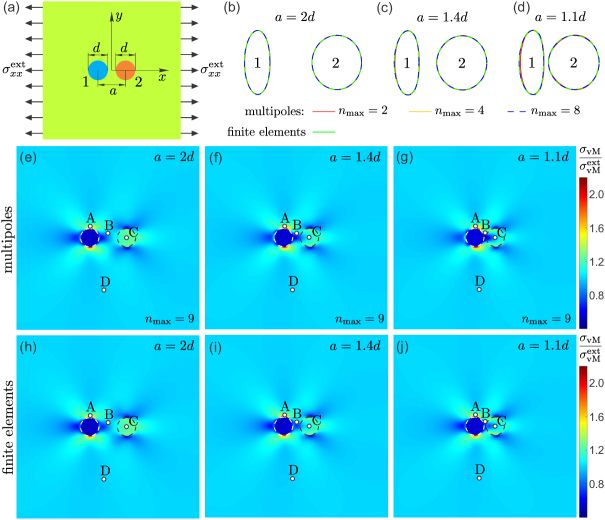
Refer to caption
Figure 5: Deformation of an infinite elastic plate with two circular inclusions under uniaxial stress σxxextsuperscriptsubscript𝜎𝑥𝑥ext\sigma_{xx}^{\text{ext}} and plane stress condition. (a) Schematic image describing the initial undeformed shape of the structure and applied load σxxext=0.25E0superscriptsubscript𝜎𝑥𝑥ext0.25subscript𝐸0\sigma_{xx}^{\text{ext}}=-0.25E_{0}. The diameters of both inclusions (blue and orange disks) are d𝑑d and the separation distance between their centers is a𝑎a. The Young’s moduli of the left and right inclusions are E1/E0=0.25subscript𝐸1subscript𝐸00.25E_{1}/E_{0}=0.25 and E2/E0=4subscript𝐸2subscript𝐸04E_{2}/E_{0}=4, respectively, where E0subscript𝐸0E_{0} is the Young’s modulus of the outer material. Poisson’s ratios of the left and right inclusions and the outer material are ν1=0.45subscript𝜈10.45\nu_{1}=0.45, ν2=0.15subscript𝜈20.15\nu_{2}=0.15, and ν0=0.3subscript𝜈00.3\nu_{0}=0.3, respectively. (b-d) Contours of the deformed inclusions for different values of the separation distance a/d=2𝑎𝑑2a/d=2, 1.41.41.4, and 1.11.11.1. The solid red, yellow and dashed blue lines show the contours obtained with elastic multipole method for nmax=2subscript𝑛max2n_{\text{max}}=2, 444, and 888, respectively. Green solid lines show the contours obtained with linear finite element simulations. (e-j) von Mises stress (σvMsubscript𝜎vM\sigma_{\text{vM}}) distributions obtained with (e-g) elastic multipole method (nmax=9subscript𝑛max9n_{\text{max}}=9) and (h-j) linear finite element simulations for different separation distances of inclusions a/d𝑎𝑑a/d. von Mises stress distributions are normalized with the value of von Mises stress σvMext=|σxxext|superscriptsubscript𝜎vMextsuperscriptsubscript𝜎𝑥𝑥ext\sigma_{\text{vM}}^{\text{ext}}=|\sigma_{xx}^{\text{ext}}| due to the applied load. Four marked points A-D were chosen for the quantitative comparison of stresses and displacements between elastic multipole method and finite element simulations. See Table 4 for details.
Refer to caption
Figure 6: Deformation of an infinite elastic plate with two circular inclusions under shear stress σxyextsuperscriptsubscript𝜎𝑥𝑦ext\sigma_{xy}^{\text{ext}} and plane stress condition. (a) Schematic image describing the initial undeformed shape of the structure and applied load σxyext=0.1E0superscriptsubscript𝜎𝑥𝑦ext0.1subscript𝐸0\sigma_{xy}^{\text{ext}}=0.1E_{0}, where E0subscript𝐸0E_{0} is the Young’s modulus of the outer material. The diameter of both inclusions (blue and orange disks) is d𝑑d and the separation distance between their centers is a𝑎a. Material properties are the same as in Fig. 5. (b-d) Contours of the deformed inclusions for different values of the separation distance a/d=2𝑎𝑑2a/d=2, 1.41.41.4, and 1.11.11.1. The solid red, yellow and dashed blue lines show the contours obtained with elastic multipole method for nmax=2subscript𝑛max2n_{\text{max}}=2, 444, and 888, respectively. Green solid lines show the contours obtained with finite element simulations. (e-j) von Mises stress (σvMsubscript𝜎vM\sigma_{\text{vM}}) distributions obtained with (e-g) elastic multipole method (nmax=9subscript𝑛max9n_{\text{max}}=9) and (h-j) linear finite element simulations for different separation distances of inclusions a/d𝑎𝑑a/d. von Mises stress distributions are normalized with the value of von Mises stress σvMext=3|σxyext|superscriptsubscript𝜎vMext3superscriptsubscript𝜎𝑥𝑦ext\sigma_{\text{vM}}^{\text{ext}}=\sqrt{3}|\sigma_{xy}^{\text{ext}}| due to the applied load. Four marked points A-D were chosen for the quantitative comparison of stresses and displacements between elastic multipole method and finite element simulation. See Table 5 for details.

Similar patterns in the von Mises stress distribution are observed when the structure is under external shear, but they are rotated by 45 (see Fig. 6e,h). When inclusions are far apart (a=2d𝑎2𝑑a=2d), the contours of deformed inclusions can be accurately described already with multipoles up to degree nmax=2subscript𝑛max2n_{\text{max}}=2 (see Figs. 5b and 6b). This degree of multipoles is sufficient because external stresses σxxextsuperscriptsubscript𝜎𝑥𝑥ext\sigma_{xx}^{\text{ext}} and σxyextsuperscriptsubscript𝜎𝑥𝑦ext\sigma_{xy}^{\text{ext}} couple only to the Fourier modes 111, cos2φi2subscript𝜑𝑖\cos 2\varphi_{i}, and sin2φi2subscript𝜑𝑖\sin 2\varphi_{i} in the expansion for stresses and displacements in Eq. (38). As the inclusions are moved closer together (a=1.4d𝑎1.4𝑑a=1.4d and a=1.1d𝑎1.1𝑑a=1.1d), they interact more strongly. As a consequence, the contours of deformed inclusions become progressively more non-elliptical and higher order of multipoles are needed to accurately describe their shapes (see Figs. 5c,d and 6c,d). Furthermore, the stress distribution inside the right inclusion becomes nonuniform (see Figs. 5f,g,i,j and 6f,g,i,j). Note that von Mises stress distributions look similar far from inclusions regardless of the separation distance a𝑎a (see Figs. 5 and 6), because they are dictated by the lowest order induced multipoles, i.e. by non-topological monopoles (p𝑝p), non-topological dipoles (𝐝psuperscript𝐝𝑝\mathbf{d}^{p}) and quadrupoles (𝐐ssuperscript𝐐𝑠\mathbf{Q}^{s}, 𝐐psuperscript𝐐𝑝\mathbf{Q}^{p}).

Table 4: Quantitative comparison for the values of von Mises stresses σvMsubscript𝜎vM\sigma_{\text{vM}} and displacements 𝐮𝐮\mathbf{u} at points A-D (defined in Fig. 5) obtained with the elastic multipole method (EMP) and finite element simulations (FEM) for uniaxially compressed samples with two inclusions of diameter d𝑑d for different values of their separation distance a𝑎a. von Mises stresses σvMsubscript𝜎vM\sigma_{\text{vM}} are normalized with the value of von Mises stress σvMext=|σxxext|superscriptsubscript𝜎vMextsuperscriptsubscript𝜎𝑥𝑥ext\sigma_{\text{vM}}^{\text{ext}}=|\sigma_{xx}^{\text{ext}}| due to the applied uniaxial compression. Displacements 𝐮𝐮\mathbf{u} are normalized with the characteristic scale of deformation dσvMext/E0𝑑superscriptsubscript𝜎vMextsubscript𝐸0d\sigma_{\text{vM}}^{\text{ext}}/E_{0}, where E0subscript𝐸0E_{0} is the Young’s modulus of the elastic matrix. The relative percent errors ϵitalic-ϵ\epsilon between the two methods are calculated as 100×(σvMEMPσvMFEM)/σvMFEM100superscriptsubscript𝜎vMEMPsuperscriptsubscript𝜎vMFEMsuperscriptsubscript𝜎vMFEM100\times(\sigma_{\text{vM}}^{\text{EMP}}-\sigma_{\text{vM}}^{\text{FEM}})/\sigma_{\text{vM}}^{\text{FEM}} and 100×(|𝐮|EMP|𝐮|FEM)/|𝐮|FEM100superscript𝐮EMPsuperscript𝐮FEMsuperscript𝐮FEM100\times(|\mathbf{u}|^{\text{EMP}}-|\mathbf{u}|^{\text{FEM}})/|\mathbf{u}|^{\text{FEM}}.
separation a=2d𝑎2𝑑a=2d separation a=1.4d𝑎1.4𝑑a=1.4d separation a=1.1d𝑎1.1𝑑a=1.1d
stress σvM/σvMextsubscript𝜎vMsuperscriptsubscript𝜎vMext\sigma_{\text{vM}}/\sigma_{\text{vM}}^{\text{ext}} disp. |𝐮|/[dσvMext/E0]𝐮delimited-[]𝑑superscriptsubscript𝜎vMextsubscript𝐸0|\mathbf{u}|/[d\sigma_{\text{vM}}^{\text{ext}}/E_{0}] stress σvM/σvMextsubscript𝜎vMsuperscriptsubscript𝜎vMext\sigma_{\text{vM}}/\sigma_{\text{vM}}^{\text{ext}} disp. |𝐮|/[dσvMext/E0]𝐮delimited-[]𝑑superscriptsubscript𝜎vMextsubscript𝐸0|\mathbf{u}|/[d\sigma_{\text{vM}}^{\text{ext}}/E_{0}] stress σvM/σvMextsubscript𝜎vMsuperscriptsubscript𝜎vMext\sigma_{\text{vM}}/\sigma_{\text{vM}}^{\text{ext}} disp. |𝐮|/[dσvMext/E0]𝐮delimited-[]𝑑superscriptsubscript𝜎vMextsubscript𝐸0|\mathbf{u}|/[d\sigma_{\text{vM}}^{\text{ext}}/E_{0}]
EMP FEM ϵitalic-ϵ\epsilon (%)(\%) EMP FEM ϵ(%)\epsilon(\%) EMP FEM ϵitalic-ϵ\epsilon (%)(\%) EMP FEM ϵ(%)\epsilon(\%) EMP FEM ϵ(%)\epsilon(\%) EMP FEM ϵ(%)\epsilon(\%)
A 1.419 1.416 0.2 1.442 1.442 0.0 1.424 1.419 0.5 1.265 1.264 0.1 1.439 1.426 0.9 1.223 1.220 0.3
B 0.940 0.947 0.7 0.082 0.081 0.5 0.940 0.959 1.9 0.116 0.116 0.7 0.887 0.91 2.7 0.127 0.126 1.0
C 1.213 1.216 0.3 0.654 0.653 0.1 1.083 1.092 0.8 0.275 0.274 0.3 0.933 0.948 1.5 0.122 0.122 0.3
D 0.997 0.997 0.0 1.144 1.144 0.0 0.994 0.994 0.0 1.250 1.250 0.0 0.992 0.992 0.0 1.363 1.363 0.0
Table 5: Quantitative comparison for the values of von Mises stresses σvMsubscript𝜎vM\sigma_{\text{vM}} and displacements 𝐮𝐮\mathbf{u} at points A-D (defined in Fig. 6) obtained with the elastic multipole method (EMP) and finite element simulations (FEM) for sheared samples with two inclusions of diameter d𝑑d for different values of their separation distance a𝑎a. von Mises stresses σvMsubscript𝜎vM\sigma_{\text{vM}} are normalized with the value of von Mises stress σvMext=3|σxyext|superscriptsubscript𝜎vMext3superscriptsubscript𝜎𝑥𝑦ext\sigma_{\text{vM}}^{\text{ext}}=\sqrt{3}|\sigma_{xy}^{\text{ext}}| due to the applied shear. Displacements 𝐮𝐮\mathbf{u} are normalized with the characteristic scale of deformation dσvMext/E0𝑑superscriptsubscript𝜎vMextsubscript𝐸0d\sigma_{\text{vM}}^{\text{ext}}/E_{0}, where E0subscript𝐸0E_{0} is the Young’s modulus of the elastic matrix. The relative percent errors ϵitalic-ϵ\epsilon between the two methods are calculated as 100×(σvMEMPσvMFEM)/σvMFEM100superscriptsubscript𝜎vMEMPsuperscriptsubscript𝜎vMFEMsuperscriptsubscript𝜎vMFEM100\times(\sigma_{\text{vM}}^{\text{EMP}}-\sigma_{\text{vM}}^{\text{FEM}})/\sigma_{\text{vM}}^{\text{FEM}} and 100×(|𝐮|EMP|𝐮|FEM)/|𝐮|FEM100superscript𝐮EMPsuperscript𝐮FEMsuperscript𝐮FEM100\times(|\mathbf{u}|^{\text{EMP}}-|\mathbf{u}|^{\text{FEM}})/|\mathbf{u}|^{\text{FEM}}.
separation a=2d𝑎2𝑑a=2d separation a=1.4d𝑎1.4𝑑a=1.4d separation a=1.1d𝑎1.1𝑑a=1.1d
stress σvM/σvMextsubscript𝜎vMsuperscriptsubscript𝜎vMext\sigma_{\text{vM}}/\sigma_{\text{vM}}^{\text{ext}} disp. |𝐮|/[dσvMext/E0]𝐮delimited-[]𝑑superscriptsubscript𝜎vMextsubscript𝐸0|\mathbf{u}|/[d\sigma_{\text{vM}}^{\text{ext}}/E_{0}] stress σvM/σvMextsubscript𝜎vMsuperscriptsubscript𝜎vMext\sigma_{\text{vM}}/\sigma_{\text{vM}}^{\text{ext}} disp. |𝐮|/[dσvMext/E0]𝐮delimited-[]𝑑superscriptsubscript𝜎vMextsubscript𝐸0|\mathbf{u}|/[d\sigma_{\text{vM}}^{\text{ext}}/E_{0}] stress σvM/σvMextsubscript𝜎vMsuperscriptsubscript𝜎vMext\sigma_{\text{vM}}/\sigma_{\text{vM}}^{\text{ext}} disp. |𝐮|/[dσvMext/E0]𝐮delimited-[]𝑑superscriptsubscript𝜎vMextsubscript𝐸0|\mathbf{u}|/[d\sigma_{\text{vM}}^{\text{ext}}/E_{0}]
EMP FEM ϵitalic-ϵ\epsilon (%)(\%) EMP FEM ϵitalic-ϵ\epsilon (%)(\%) EMP FEM ϵitalic-ϵ\epsilon (%)(\%) EMP FEM ϵitalic-ϵ\epsilon (%)(\%) EMP FEM ϵitalic-ϵ\epsilon (%)(\%) EMP FEM ϵitalic-ϵ\epsilon (%)(\%)
A 1.027 1.026 0.1 1.167 1.166 0.1 1.051 1.047 0.4 1.132 1.131 0.1 1.085 1.076 0.9 1.159 1.156 0.2
B 1.045 1.050 0.5 0.387 0.387 0.2 1.065 1.081 1.5 0.379 0.377 0.5 1.106 1.134 2.5 0.371 0.368 0.8
C 1.415 1.419 0.2 0.159 0.159 0.0 1.469 1.481 0.8 0.280 0.279 0.2 1.512 1.533 1.4 0.407 0.405 0.4
D 1.016 1.016 0.0 4.235 4.235 0.0 1.016 1.016 0.0 4.265 4.265 0.0 1.020 1.020 0.0 4.275 4.275 0.0
Refer to caption
Figure 7: Normalized errors and amplitudes of induced multipoles for the structures with two inclusions with diameters d𝑑d and the separation distance a𝑎a under (a) uniaxial stress σxxextsuperscriptsubscript𝜎𝑥𝑥ext\sigma_{xx}^{\text{ext}} (see Fig. 5) and (b) shear stress σxyextsuperscriptsubscript𝜎𝑥𝑦ext\sigma_{xy}^{\text{ext}} (see Fig. 6). The normalized errors for displacements ϵdisp(nmax)subscriptitalic-ϵdispsubscript𝑛max\epsilon_{\text{disp}}(n_{\text{max}}) (blue lines) and stresses ϵstress(nmax)subscriptitalic-ϵstresssubscript𝑛max\epsilon_{\text{stress}}(n_{\text{max}}) (red lines) are defined in Eq. (40). Absolute values of the amplitudes of induced multipoles {𝐚1,out,𝐚2,out}subscript𝐚1outsubscript𝐚2out\{\mathbf{a}_{1,\text{out}},\mathbf{a}_{2,\text{out}}\} for nmax=9subscript𝑛max9n_{\text{max}}=9. In (a) the amplitudes are normalized as a~n=an/σxxextsubscript~𝑎𝑛subscript𝑎𝑛superscriptsubscript𝜎𝑥𝑥ext\tilde{a}_{n}=a_{n}/\sigma_{xx}^{\text{ext}}, c~n=cn/σxxextsubscript~𝑐𝑛subscript𝑐𝑛superscriptsubscript𝜎𝑥𝑥ext\tilde{c}_{n}=c_{n}/\sigma_{xx}^{\text{ext}}, A~n=An/σxxextsubscript~𝐴𝑛subscript𝐴𝑛superscriptsubscript𝜎𝑥𝑥ext\tilde{A}_{n}=A_{n}/\sigma_{xx}^{\text{ext}}, and C~n=Cn/σxxextsubscript~𝐶𝑛subscript𝐶𝑛superscriptsubscript𝜎𝑥𝑥ext\tilde{C}_{n}=C_{n}/\sigma_{xx}^{\text{ext}}. The dark and light blue colored bars correspond to the positive (an,cn,An,Cn>0subscript𝑎𝑛subscript𝑐𝑛subscript𝐴𝑛subscript𝐶𝑛0a_{n},c_{n},A_{n},C_{n}>0) and negative (an,cn,An,Cn<0subscript𝑎𝑛subscript𝑐𝑛subscript𝐴𝑛subscript𝐶𝑛0a_{n},c_{n},A_{n},C_{n}<0) amplitudes for inclusion 1, respectively. Similarly, the red and orange colored bars correspond to the positive and negative amplitudes for inclusion 2, respectively. Note that the amplitudes of multipoles bisubscript𝑏𝑖b_{i}, disubscript𝑑𝑖d_{i}, Bisubscript𝐵𝑖B_{i}, and Disubscript𝐷𝑖D_{i} are zero due to the symmetry of the problem. In (b) the amplitudes are normalized as b~n=bn/σxyextsubscript~𝑏𝑛subscript𝑏𝑛superscriptsubscript𝜎𝑥𝑦ext\tilde{b}_{n}=b_{n}/\sigma_{xy}^{\text{ext}}, d~n=dn/σxyextsubscript~𝑑𝑛subscript𝑑𝑛superscriptsubscript𝜎𝑥𝑦ext\tilde{d}_{n}=d_{n}/\sigma_{xy}^{\text{ext}}, B~n=Bn/σxyextsubscript~𝐵𝑛subscript𝐵𝑛superscriptsubscript𝜎𝑥𝑦ext\tilde{B}_{n}=B_{n}/\sigma_{xy}^{\text{ext}}, and D~n=Dn/σxyextsubscript~𝐷𝑛subscript𝐷𝑛superscriptsubscript𝜎𝑥𝑦ext\tilde{D}_{n}=D_{n}/\sigma_{xy}^{\text{ext}}. The dark and light blue colored bars correspond to the positive (bn,dn,Bn,Dn>0subscript𝑏𝑛subscript𝑑𝑛subscript𝐵𝑛subscript𝐷𝑛0b_{n},d_{n},B_{n},D_{n}>0) and negative (bn,dn,Bn,Dn<0subscript𝑏𝑛subscript𝑑𝑛subscript𝐵𝑛subscript𝐷𝑛0b_{n},d_{n},B_{n},D_{n}<0) amplitudes for inclusion 1, respectively. Similarly, the red and orange colored bars correspond to the positive and negative amplitudes for inclusion 2, respectively. Note that the amplitudes of multipoles aisubscript𝑎𝑖a_{i}, cisubscript𝑐𝑖c_{i}, Aisubscript𝐴𝑖A_{i}, and Cisubscript𝐶𝑖C_{i} are zero due to the symmetry of the problem.

To determine the proper number for the maximum degree nmaxsubscript𝑛maxn_{\text{max}} of induced multipoles we performed a convergence analysis for the spatial distributions of displacements 𝐮(nmax)(x,y)superscript𝐮subscript𝑛max𝑥𝑦\mathbf{u}^{(n_{\text{max}})}(x,y) and von Mises stresses σvM(nmax)(x,y)subscriptsuperscript𝜎subscript𝑛maxvM𝑥𝑦\sigma^{(n_{\text{max}})}_{\text{vM}}(x,y). Displacements and von Mises stresses were evaluated at Np=1001×1001subscript𝑁𝑝10011001N_{p}=1001\times 1001 points on a square grid of size 10d×10d10𝑑10𝑑10d\times 10d surrounding the inclusions, i.e. at the points (xi,yj)=(id/100,jd/100)subscript𝑥𝑖subscript𝑦𝑗𝑖𝑑100𝑗𝑑100(x_{i},y_{j})=\left(id/100,jd/100\right), where i,j{500,499,,500}𝑖𝑗500499500i,j\in\{-500,-499,\ldots,500\}. The normalized errors for displacements ϵdisp(nmax)subscriptitalic-ϵdispsubscript𝑛max\epsilon_{\text{disp}}(n_{\text{max}}) and stresses ϵstress(nmax)subscriptitalic-ϵstresssubscript𝑛max\epsilon_{\text{stress}}(n_{\text{max}}) were obtained by calculating the relative changes of the spatial distributions of displacements and von Mises stresses when the maximum degree nmaxsubscript𝑛maxn_{\text{max}} of induced multipoles is increased by one. The normalized errors are given by SpecMethod

ϵdisp(nmax)subscriptitalic-ϵdispsubscript𝑛max\displaystyle\epsilon_{\text{disp}}(n_{\text{max}}) =1Np[i,j|(𝐮(nmax+1)(xi,yj)𝐮(nmax)(xi,yj)dσvMext/E0)2|]1/2,absent1subscript𝑁𝑝superscriptdelimited-[]subscript𝑖𝑗superscriptsuperscript𝐮subscript𝑛max1subscript𝑥𝑖subscript𝑦𝑗superscript𝐮subscript𝑛maxsubscript𝑥𝑖subscript𝑦𝑗𝑑superscriptsubscript𝜎vMextsubscript𝐸0212\displaystyle=\frac{1}{\sqrt{N_{p}}}\left[\sum_{i,j}\left|\left(\frac{\mathbf{u}^{(n_{\text{max}}+1)}(x_{i},y_{j})-\mathbf{u}^{(n_{\text{max}})}(x_{i},y_{j})}{d\,\sigma_{\text{vM}}^{\text{ext}}/E_{0}}\right)^{2}\right|\right]^{1/2}, (40a)
ϵstress(nmax)subscriptitalic-ϵstresssubscript𝑛max\displaystyle\epsilon_{\text{stress}}(n_{\text{max}}) =1Np[i,j(σvM(nmax+1)(xi,yj)σvM(nmax)(xi,yj)σvMext)2]1/2.absent1subscript𝑁𝑝superscriptdelimited-[]subscript𝑖𝑗superscriptsubscriptsuperscript𝜎subscript𝑛max1vMsubscript𝑥𝑖subscript𝑦𝑗subscriptsuperscript𝜎subscript𝑛maxvMsubscript𝑥𝑖subscript𝑦𝑗superscriptsubscript𝜎vMext212\displaystyle=\frac{1}{\sqrt{N_{p}}}\left[\sum_{i,j}\left(\frac{\sigma^{(n_{\text{max}}+1)}_{\text{vM}}(x_{i},y_{j})-\sigma^{(n_{\text{max}})}_{\text{vM}}(x_{i},y_{j})}{\sigma_{\text{vM}}^{\text{ext}}}\right)^{2}\right]^{1/2}. (40b)

Here, displacements and von Mises stresses are normalized by the characteristic scales dσvMext/E0𝑑superscriptsubscript𝜎vMextsubscript𝐸0d\sigma_{\text{vM}}^{\text{ext}}/E_{0} and σvMextsuperscriptsubscript𝜎vMext\sigma_{\text{vM}}^{\text{ext}}, respectively, where d𝑑d is the diameter of inclusions, σvMextsuperscriptsubscript𝜎vMext\sigma_{\text{vM}}^{\text{ext}} is the value of the von Mises stress due to external load, and E0subscript𝐸0E_{0} is the Young’s modulus of the surrounding matrix. The normalized errors are plotted in Fig. 7. As the maximum degree nmaxsubscript𝑛maxn_{\text{max}} of induced multipoles is increased, the normalized errors for displacements ϵdisp(nmax)subscriptitalic-ϵdispsubscript𝑛max\epsilon_{\text{disp}}(n_{\text{max}}) and stresses ϵstress(nmax)subscriptitalic-ϵstresssubscript𝑛max\epsilon_{\text{stress}}(n_{\text{max}}) decrease exponentially. Since the induced elastic multipoles form the basis for the biharmonic equation, this is akin to the spectral method, which is exponentially convergent when the functions and the boundaries are smooth SpecMethod . The normalized errors for displacements are lower than the errors for stresses (see Fig. 7) because stresses are related to spatial derivatives of displacements. Note that the normalized errors decrease more slowly when inclusions are brought close together and their interactions become important (see Fig. 7). This is also reflected in the amplitudes 𝐚1,insubscript𝐚1in\mathbf{a}_{1,\text{in}}, 𝐚2,insubscript𝐚2in\mathbf{a}_{2,\text{in}}, 𝐚1,outsubscript𝐚1out\mathbf{a}_{1,\text{out}}, and 𝐚2,outsubscript𝐚2out\mathbf{a}_{2,\text{out}} of the induced multipoles, which decrease exponentially with the degree of multipoles and they decrease more slowly when inclusions are closer (see Fig. 7).

Results from the elastic multipole method were compared with linear finite element simulations, and very good agreement is achieved already for nmax=9subscript𝑛max9n_{\text{max}}=9 even when inclusions are very close together (a=1.1d𝑎1.1𝑑a=1.1d, see Figs. 5 and 6). To make the comparison with finite elements more quantitative, we compared the values of displacements and stresses at 4 different points: A – at the edge of the left inclusion, B – in between the inclusions, C – at the center of the right inclusion, and D – far away from both inclusions (see Figs. 5 and 6). For all 4 points, the error increases when inclusions are brought closer together (see Tables 4 and 5). Of the 4 different points, we find that the errors are the largest at point B, which is strongly influenced by induced multipoles from both inclusions. For the smallest separation distance a=1.1d𝑎1.1𝑑a=1.1d between the inclusions, the errors for the von Mises stress at point B are 2.7%percent2.72.7\% and 2.5%percent2.52.5\% for the uniaxial and shear loads, respectively. These errors can be further reduced by increasing the number nmaxsubscript𝑛maxn_{\text{max}} for the maximum degree of multipoles, e.g. for nmax=14subscript𝑛max14n_{\text{max}}=14 the errors for von Mises stress at point B are reduced to 1.2%percent1.21.2\% and 1.1%percent1.11.1\% for the uniaxial and shear loads, respectively.
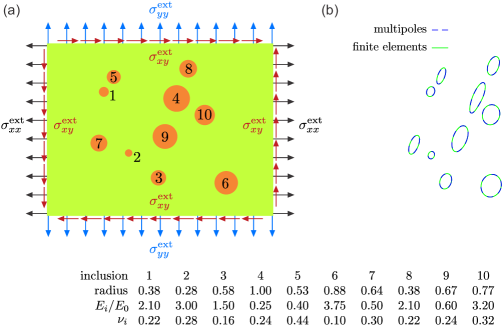
Refer to caption
Figure 8: Deformation of an infinite elastic plate with ten circular inclusions (orange disks) under general external stress. (a) Schematic image describing the initial undeformed shape of the structure and applied external loads: σxxext/E0=0.25superscriptsubscript𝜎𝑥𝑥extsubscript𝐸00.25\sigma_{xx}^{\text{ext}}/E_{0}=-0.25, σyyext/E0=0.05superscriptsubscript𝜎𝑦𝑦extsubscript𝐸00.05\sigma_{yy}^{\text{ext}}/E_{0}=0.05, and σxyext/E0=0.10superscriptsubscript𝜎𝑥𝑦extsubscript𝐸00.10\sigma_{xy}^{\text{ext}}/E_{0}=0.10, where E0subscript𝐸0E_{0} is the Young’s modulus of the outer material. The plane stress condition was used. The radii and material properties (Young’s moduli Eisubscript𝐸𝑖E_{i} and Poisson’s ratios νisubscript𝜈𝑖\nu_{i}) of inclusions are provided in the table below the schematic image. The radii of inclusions are normalized by the radius of the largest inclusion. The Young’s moduli are normalized by the Young’s modulus of the outer material E0subscript𝐸0E_{0}. The value of Poisson’s ratio for the outer material was ν0=0.3subscript𝜈00.3\nu_{0}=0.3. (b) Contours of deformed inclusions. The blue dashed lines show the results obtained with the elastic multipole method (nmax=6subscript𝑛max6n_{\text{max}}=6). The green solid lines correspond to the deformed contours obtained with linear finite element simulations.

To demonstrate the full potential of the elastic multipole method, we also considered the deformation of an infinite plate with N=10𝑁10N=10 inclusions of different sizes and material properties subjected to general external stress load under plane stress condition (see Fig. 8). The contours of deformed inclusions obtained with finite element simulations (green solid lines) and elastic multipole method with nmax=6subscript𝑛max6n_{\text{max}}=6 (blue dashed lines) are in very good agreement. Note that the results for the elastic multipole method were obtained by solving the linear system of only N(8nmax2)=460𝑁8subscript𝑛max2460N(8n_{\text{max}}-2)=460 equations for the amplitudes of the induced multipoles described in Eq. (39), which is significantly smaller than the number of degrees of freedom required for finite element simulations.

III.3 Comparison with experiments

Finally, we also tested the elastic multipole method against experiments. Experimental samples were prepared by casting Elite Double 32 (Zhermack) elastomers with the measured Young’s modulus E0=0.97subscript𝐸00.97E_{0}=0.97 MPa and assumed Poisson’s ratio ν=0.49𝜈0.49\nu=0.49 babaee20133d . Molds were fabricated from 5 mm thick acrylic plates with laser-cut circular holes, which were then filled with acrylic cylinders in the assembled molds to create cylindrical holes in the elastomer samples. Approximately 30 min after casting, the molds were disassembled and the solid samples were placed in a convection oven at 40 C for 12 hours for further curing. The cylindrical inclusions made from acrylic (Young’s modulus E=2.9𝐸2.9E=2.9 GPa, Poisson’s ratio ν=0.37𝜈0.37\nu=0.37 acrylic ) were inserted into the holes of the elastomer samples and they were glued by a cyanoacrylate adhesive.

Refer to caption
Figure 9: Experimental systems for displacement controlled compressive tests. (a) A mechanism for compression of rubber samples (green slab) sits on top of a flatbed photo scanner, which is used to extract the contours of deformed holes/inclusions. The zoomed-in photo on the left shows a 3D-printed plastic wrench that was used for the precise control of screw turns. (b) Setup for extracting strain fields via digital image correlation (DIC). The surface of the sample was painted with speckle patterns. The sample was then compressed with steel plates of the testing machine and photos of speckle patterns were used to extract the displacement field on the front surface of the slab. The zoomed-in photo on the right shows the rubber sample with one hole and one inclusion (indicated with a red dashed circle) mounted between two parallel plates of the testing machine.

We designed two compressive testing systems (see Fig. 9) to compare the contours of deformed holes and inclusions and strain fields with predictions made by the elastic multipole method. In Fig. 9a, we first present an experimental system for extracting the contours of deformed holes and inclusions in compressed experimental samples. The system comprises a custom-made loading mechanism and a flatbed photo scanner. Displacement loading is applied in 0.5 mm increments via 180superscript180180^{\circ} turns of the M10x1 screw (metric thread with 10 mm diameter and 1 mm pitch) in the mechanism, which is controlled by a 3D-printed plastic wrench (see the inset of Fig. 9a). The loading mechanism was placed on an Epson V550 photo scanner to scan the surface of deformed samples and silicone oil was applied between the sample and the glass surface of the scanner to reduce friction between them. Scanned images were post-processed with Corel PHOTO-PAINT X8 and the Image Processing Toolbox in MATLAB 2018b. First, the dust particles and air bubbles trapped in a thin film of silicone oil were digitally removed from the scanned images. Scanned grayscale images were then converted to black and white binary images from which the contours were obtained with MATLAB.

Second, we present a system for capturing the displacement and strain fields in compressed samples via digital image correlation (DIC) technique (see Fig. 9b). Black and white speckle patterns were spray-painted onto the surface of samples with slow-drying acrylic paint to prevent the speckle pattern from hardening too quickly, which could lead to delamination under applied compressive loads. Using a Zwick Z050 universal material testing machine, we applied a compressive displacement in 0.2 mm increments, where again a silicone oil was applied between the steel plates and the elastomer samples to prevent sticking and to reduce friction. A Nikon D5600 photo camera was used at each step to take a snapshot of the compressed sample (see Fig. 9b). These photos were then used to calculate the displacements and strain fields with Ncorr, an open-source 2D DIC MATLAB based software. DIC

We analyzed uniaxially compressed 100 mm×100 mm×25 mm100 mm100 mm25 mm100\text{ mm}\times 100\text{ mm}\times 25\text{ mm} elastomer structures with three different configurations (horizontal, vertical and inclined at 45superscript4545^{\circ} angle) of two holes with identical diameters d=8.11𝑑8.11d=8.11 mm and their separation distance a=9.50𝑎9.50a=9.50 mm (see Fig. 10a-c). Holes were placed near the centers of elastomer structures to minimize the effects of boundaries. The structures were relatively thick (252525 mm) to prevent the out-of-plane buckling. The contours of deformed holes in compressed experimental samples under external strain εyyext=0.05superscriptsubscript𝜀𝑦𝑦ext0.05\varepsilon_{yy}^{\text{ext}}=-0.05 were compared with those obtained with elastic multipole method and finite element simulations (see Fig. 10d-f). For the elastic multipole method, we used external stress σyyext=E0εyyextsuperscriptsubscript𝜎𝑦𝑦extsubscript𝐸0superscriptsubscript𝜀𝑦𝑦ext\sigma_{yy}^{\text{ext}}=E_{0}\varepsilon_{yy}^{\text{ext}} (σxxextσxyext0superscriptsubscript𝜎𝑥𝑥extsuperscriptsubscript𝜎𝑥𝑦ext0\sigma_{xx}^{\text{ext}}\approx\sigma_{xy}^{\text{ext}}\approx 0 due to reduced friction) and plane stress condition was assumed since the experimental samples were free to expand in the out-of-plane direction. Linear finite element simulations were performed for finite-size (100 mm×100 mm100 mm100 mm100\text{ mm}\times 100\text{ mm}) 2D structures with circular holes under plane stress condition. In finite element simulations, samples were compressed by prescribing a uniform displacement in the y𝑦y-direction on the upper and lower surfaces, while allowing nodes on these surfaces to move freely in the x𝑥x-direction. The midpoint of the bottom edge was constrained to prevent rigid body translations in the x𝑥x-direction.

Refer to caption
Figure 10: Uniaxial vertical compression of elastic structures with holes and inclusions. (a-c) Schematic images describing the initial undeformed shapes of structures with two holes (white disks) in three different configurations (horizontal, vertical and inclined at 45superscript4545^{\circ}) and applied external strain εyyext=0.05superscriptsubscript𝜀𝑦𝑦ext0.05\varepsilon_{yy}^{\text{ext}}=-0.05. Deformed contours of holes obtained with elastic multipole method (nmax=10subscript𝑛max10n_{\text{max}}=10, blue dashed lines), experiments (orange solid lines), and finite element simulations (solid green lines). (d-f) Schematic images describing the initial undeformed shapes of structures with one hole (white disks) and one inclusion (orange disks) in three different configurations (horizontal, vertical and inclined at 45superscript4545^{\circ}), and applied external strain εyyext=0.05superscriptsubscript𝜀𝑦𝑦ext0.05\varepsilon_{yy}^{\text{ext}}=-0.05. Deformed contours of holes and inclusions obtained with elastic multipole method (nmax=10subscript𝑛max10n_{\text{max}}=10, blue dashed lines), experiments (orange solid lines), and finite element simulations (solid green lines). In all cases, the size of samples was 100 mm×100 mm×25 mm100 mm100 mm25 mm100\text{ mm}\times 100\text{ mm}\times 25\text{ mm}, the diameters of each hole/inclusion were d=8.11 mm𝑑8.11 mmd=8.11\text{ mm}, and their separation distances were a=9.50 mm𝑎9.50 mma=9.50\text{ mm}.
Refer to caption
Figure 11: Equivalent von Mises strain fields εvMsubscript𝜀vM\varepsilon_{\text{vM}} (see Eq. (41)) for uniaxially vertically compressed elastic structures with two holes (white disks) in three different configurations (horizontal, vertical, inclined at 45superscript4545^{\circ}) introduced in Fig. 10. Equivalent von Mises strain fields εvMsubscript𝜀vM\varepsilon_{\text{vM}} were obtained with (a-c) elastic multipole method (nmax=10subscript𝑛max10n_{\text{max}}=10), (d-f) finite element simulations, and (g-i) DIC analysis of experiments. Note that the strain data was corrupted near the edges for some samples due to oil stains on the speckle patterns near the boundary. For this reason, we omitted the affected border regions (grey frames) in heat maps (g-i). Four marked points A-D were chosen for the quantitative comparison of strains εvMsubscript𝜀vM\varepsilon_{\text{vM}}. See Table 6 for details.

The contours of deformed holes obtained in experiments agree very well with those obtained with elastic multipole method (nmax=10subscript𝑛max10n_{\text{max}}=10) and linear finite element simulations for all three configurations of holes (see Fig. 10a-c). We also compared the equivalent von Mises strain fields defined as Barber

εvM=σvME=11+νεxx2εxxεyy+εyy2+3εxy2+ν(1ν)2(εxx+εyy)2subscript𝜀vMsubscript𝜎vM𝐸11𝜈superscriptsubscript𝜀𝑥𝑥2subscript𝜀𝑥𝑥subscript𝜀𝑦𝑦superscriptsubscript𝜀𝑦𝑦23superscriptsubscript𝜀𝑥𝑦2𝜈superscript1𝜈2superscriptsubscript𝜀𝑥𝑥subscript𝜀𝑦𝑦2\varepsilon_{\text{vM}}=\frac{\sigma_{\text{vM}}}{E}=\frac{1}{1+\nu}\sqrt{\varepsilon_{xx}^{2}-\varepsilon_{xx}\varepsilon_{yy}+\varepsilon_{yy}^{2}+3\varepsilon_{xy}^{2}+\frac{\nu}{(1-\nu)^{2}}(\varepsilon_{xx}+\varepsilon_{yy})^{2}} (41)

that were obtained with elastic multipole method (nmax=10subscript𝑛max10n_{\text{max}}=10), finite element simulations, and DIC analyses of experiments (see Fig. 11). For all three configurations of holes, the strain fields agree very well between the elastic multipole method (Fig. 11a-c) and finite element simulations (Fig. 11d-f). The strain fields for experimental samples are qualitatively similar, but they differ quantitatively near the holes as can be seen from heat maps in Fig. 11g-i. The quantitative comparison of strains at four different points A-D (marked in Fig. 11) showed a relative error of 2224%percent44\% between elastic multipole method and finite elements, and a relative error of 0014%percent1414\% between elastic multipole method and experiments (see Table 6). The discrepancy between elastic multipole method and finite element simulations is attributed to the finite size effects. For elastic multipole method, we assumed an infinite domain, while finite domains were modeled in finite element simulations to mimic experiments. Since the domains are relatively small, interactions of induced elastic multipoles with boundaries become important, which is discussed in detail in the companion paper sarkar2020image . The discrepancy between experiments and elastic multipole method is also attributed to the confounding effects of nonlinear deformation due to moderately large compression (εyyext=0.05superscriptsubscript𝜀𝑦𝑦ext0.05\varepsilon_{yy}^{\text{ext}}=-0.05), 3D deformation due to relatively thick samples, fabrication imperfections, nonzero friction between the sample and the mounting grips of the testing machine, the alignment of camera with the sample (2D DIC system was used), and the errors resulting from the choice of DIC parameters (see e.g. YuPan ; Sutton ).
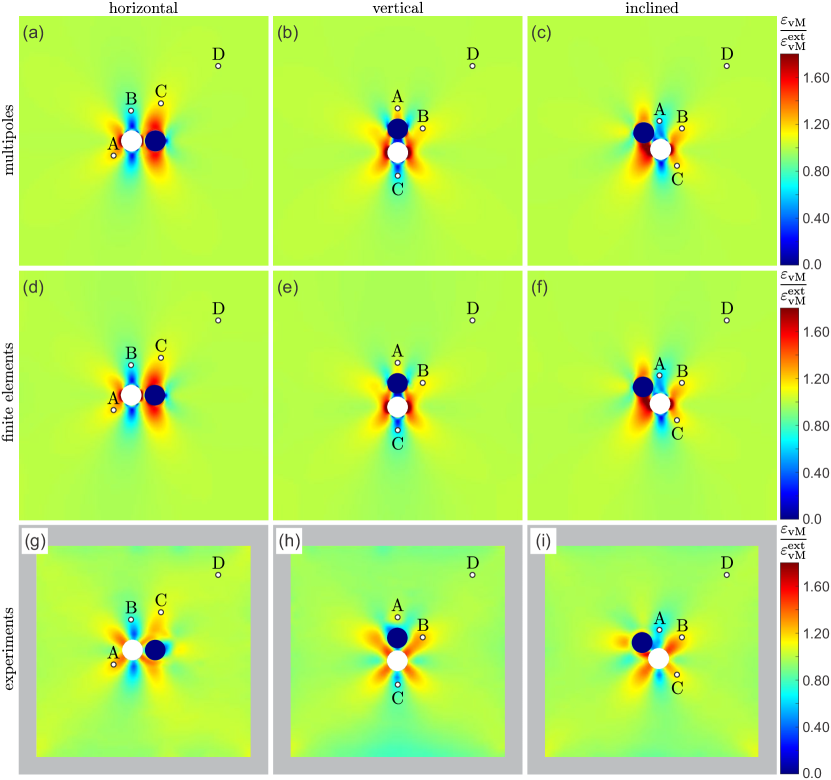
Refer to caption
Figure 12: Equivalent von Mises strain fields εvMsubscript𝜀vM\varepsilon_{\text{vM}} (see Eq. (41)) for uniaxially vertically compressed elastic structures with one hole (white disks) and one inclusion (blue disks) in three different configurations (horizontal, vertical, inclined at 45superscript4545^{\circ}) introduced in Fig. 10. Equivalent von Mises strain fields εvMsubscript𝜀vM\varepsilon_{\text{vM}} were obtained with (a-c) elastic multipole method (nmax=10subscript𝑛max10n_{\text{max}}=10), (d-f) linear finite element simulations, and (g-i) DIC analysis of experiments. Note that the strain data was corrupted near the edges for some samples due to oil stains on the speckle patterns near the boundary. For this reason, we omitted the affected border regions (grey frames) in heat maps (g-i). Four marked points A-D were chosen for the quantitative comparison of strains εvMsubscript𝜀vM\varepsilon_{\text{vM}}. See Table 7 for details.
Table 6: Quantitative comparison for the values of equivalent von Mises strains εvMsubscript𝜀vM\varepsilon_{\text{vM}} normalized with the value for the applied external load εvMextsuperscriptsubscript𝜀vMext\varepsilon_{\text{vM}}^{\text{ext}} at points A-D (defined in Fig. 11) in compressed samples with two holes in three different configurations (horizontal, vertical, inclined) obtained with elastic multipole method (EMP), finite element simulations (FEM) and DIC analysis of experiments (EXP). The relative percent errors between EMP and FEM were calculated as 100×(εvM(EMP)εvM(FEM))/εvM(FEM)100superscriptsubscript𝜀vM(EMP)superscriptsubscript𝜀vM(FEM)superscriptsubscript𝜀vM(FEM)100\times(\varepsilon_{\text{vM}}^{\text{(EMP)}}-\varepsilon_{\text{vM}}^{\text{(FEM)}})/\varepsilon_{\text{vM}}^{\text{(FEM)}}. The relative percent errors between EMP and EXP were calculated as 100×(εvM(EMP)εvM(EXP))/εvM(EXP)100superscriptsubscript𝜀vM(EMP)superscriptsubscript𝜀vM(EXP)superscriptsubscript𝜀vM(EXP)100\times(\varepsilon_{\text{vM}}^{\text{(EMP)}}-\varepsilon_{\text{vM}}^{\text{(EXP)}})/\varepsilon_{\text{vM}}^{\text{(EXP)}}.
points horizontal vertical inclined
strain εvM/ϵvMextsubscript𝜀vMsuperscriptsubscriptitalic-ϵvMext\varepsilon_{\text{vM}}/\epsilon_{\text{vM}}^{\text{ext}} error of EMP (%) strain εvM/ϵvMextsubscript𝜀vMsuperscriptsubscriptitalic-ϵvMext\varepsilon_{\text{vM}}/\epsilon_{\text{vM}}^{\text{ext}} error of EMP (%) strain εvM/ϵvMextsubscript𝜀vMsuperscriptsubscriptitalic-ϵvMext\varepsilon_{\text{vM}}/\epsilon_{\text{vM}}^{\text{ext}} error of EMP (%)
EMP FEM EXP FEM EXP EMP FEM EXP FEM EXP EMP FEM EXP FEM EXP
A 1.17 1.14 1.17 2.6 0.2 1.14 1.12 1.12 2.0 2.3 1.19 1.16 1.18 2.6 0.7
B 1.07 1.04 1.11 2.7 3.8 0.71 0.69 0.73 2.0 3.3 0.63 0.61 0.63 3.9 0.3
C 1.05 1.03 0.92 2.5 14.1 1.23 1.21 1.12 1.7 10.2 1.21 1.18 1.15 2.7 4.9
D 1.03 1.00 0.98 2.8 4.5 1.02 1.00 1.00 1.6 2.0 1.03 1.00 0.99 2.8 4.2
Table 7: Quantitative comparison for the values of equivalent von Mises strains εvMsubscript𝜀vM\varepsilon_{\text{vM}} normalized with the value for the applied external load εvMextsuperscriptsubscript𝜀vMext\varepsilon_{\text{vM}}^{\text{ext}} at points A-D (defined in Fig. 12) in compressed samples with one hole and one inclusion in three different configurations (horizontal, vertical, inclined) obtained with elastic multipole method (EMP), finite element simulations (FEM) and DIC analysis of experiments (EXP). The relative percent errors between EMP and FEM were calculated as 100×(εvM(EMP)εvM(FEM))/εvM(FEM)100superscriptsubscript𝜀vM(EMP)superscriptsubscript𝜀vM(FEM)superscriptsubscript𝜀vM(FEM)100\times(\varepsilon_{\text{vM}}^{\text{(EMP)}}-\varepsilon_{\text{vM}}^{\text{(FEM)}})/\varepsilon_{\text{vM}}^{\text{(FEM)}}. The relative percent errors between EMP and EXP were calculated as 100×(εvM(EMP)εvM(EXP))/εvM(EXP)100superscriptsubscript𝜀vM(EMP)superscriptsubscript𝜀vM(EXP)superscriptsubscript𝜀vM(EXP)100\times(\varepsilon_{\text{vM}}^{\text{(EMP)}}-\varepsilon_{\text{vM}}^{\text{(EXP)}})/\varepsilon_{\text{vM}}^{\text{(EXP)}}.
points horizontal vertical inclined
strain εvM/ϵvMextsubscript𝜀vMsuperscriptsubscriptitalic-ϵvMext\varepsilon_{\text{vM}}/\epsilon_{\text{vM}}^{\text{ext}} error of EMP (%) strain εvM/ϵvMextsubscript𝜀vMsuperscriptsubscriptitalic-ϵvMext\varepsilon_{\text{vM}}/\epsilon_{\text{vM}}^{\text{ext}} error of EMP (%) strain εvM/ϵvMextsubscript𝜀vMsuperscriptsubscriptitalic-ϵvMext\varepsilon_{\text{vM}}/\epsilon_{\text{vM}}^{\text{ext}} error of EMP (%)
EMP FEM EXP FEM EXP EMP FEM EXP FEM EXP EMP FEM EXP FEM EXP
A 1.21 1.20 1.23 0.7 1.1 1.11 1.07 1.06 3.9 4.5 0.61 0.59 0.57 4.8 7.0
B 0.70 0.70 0.62 0.6 11.9 1.14 1.14 1.27 0.5 10.1 1.18 1.15 1.18 2.4 0.5
C 1.14 1.13 1.09 0.7 4.0 0.57 0.56 0.61 1.4 6.3 1.16 1.15 1.17 0.7 1.2
D 1.01 1.00 0.97 0.2 3.7 1.00 0.99 0.97 1.0 3.3 1.00 0.99 0.96 0.8 4.0

Experiments were repeated with relatively rigid inclusions (Einc/E0=3000subscript𝐸incsubscript𝐸03000E_{\text{inc}}/E_{0}=3000), where the samples described above were reused. Acrylic (PMMA) rods were inserted into one of the holes and glued with a cyanoacrylate adhesive for each of the samples. The contours of deformed holes obtained in experiments matched very well with those obtained with elastic multipole method (nmax=10subscript𝑛max10n_{\text{max}}=10) and finite element simulations for all three configurations of holes and inclusions (see Fig. 10d-f). A relatively good agreement was also obtained for strain fields (see Fig. 12), where the strains inside rigid inclusions are very small (dark blue color). The quantitative comparison of strains at four different points A-D (marked in Fig. 12) showed a relative error of 00-5%percent55\% between elastic multipole method and finite elements, and a relative error of 00-12%percent1212\% between elastic multipole method and experiments (see Table 7).

IV Conclusion

In this paper, we demonstrated how induction and multipole expansion, which are common concepts in electrostatics, can be effectively used also for analyzing the linear deformation of infinite 2D elastic structures with circular holes and inclusions for both plane stress and plane strain conditions. Unlike in electrostatics, there are two different types of multipoles 𝐐nssuperscriptsubscript𝐐𝑛𝑠\mathbf{Q}_{n}^{s} and 𝐐npsuperscriptsubscript𝐐𝑛𝑝\mathbf{Q}_{n}^{p} in elasticity, which are derived from topological monopoles s𝑠s (disclinations) and non-topological monopoles p𝑝p. This is due to the biharmonic nature of the Airy stress function. The external load can induce all of these multipoles except for the topological defects called disclinations (topological monopole s𝑠s) and dislocations (topological dipole 𝐝ssuperscript𝐝𝑠\mathbf{d}^{s}).

The multipole expansion is a so-called far-field method and is thus extremely efficient when holes and inclusions are far apart. In this case, very accurate results can be obtained by considering only induced quadrupoles, because the effect of higher-order multipoles decays more rapidly at large distances. When holes and inclusions are closer together, their interactions via induced higher-order multipoles become important as well. The accuracy of the results increases exponentially with the maximum degree of elastic multipoles, which is also the case in electrostatics, and this is characteristic for spectral methods SpecMethod .

Note that the Stokes flows in 2D can also be described in terms of the biharmonic equations of the stream function Stream . Hence, it may seem that the multipole method described above could be adapted for Stokes flows around rigid and deformable obstacles. However, this is not possible due to the Stokes’ paradox, which is the phenomenon that there can be no creeping flow of a fluid around a disk in 2D Stream .

The elastic multipole method presented here was limited to deformations of infinite structures with holes and inclusions of circular shapes. It can be generalized to deformations of finite size structures by employing the concept of image charges from electrostatics, which is discussed in detail in the companion paper sarkar2020image . This method can also be adapted to describe deformations of structures with non-circular holes and inclusions, and can in principle be generalized to describe deformations of curved thin shells with inclusions.

While the elastic multipole method presented here focused only on linear deformation, similar concepts can also be useful for describing the post-buckling deformation of mechanical metamaterials. Previously, it was demonstrated that the buckled patterns of structures with periodic arrays of holes Kamien ; matsumoto2012patterns ; Auxetic ; Moshe3 , square frames Moshe4 ; Moshe5 and kirigami slits Moshe4 can be qualitatively described with interacting quadrupoles. Furthermore, the approach with elastic quadrupoles has recently been extended to the nonlinear regime of compressed structures with periodic arrays of holes, which can estimate the initial linear deformation, the critical buckling load, as well as the buckling mode Moshe6 . The accuracy of these results could be further improved by expanding the induced fields to higher-order multipoles. Thus, the elastic multipole method has the potential to significantly advance our understanding of deformation patterns in structures with holes and inclusions.

Acknowledgements

This work was supported by NSF through the Career Award DMR-1752100 and by the Slovenian Research Agency through the grant P2-0263. We would like to acknowledge useful discussions with Michael Moshe (Hebrew University) and thank Jonas Trojer (University of Ljubljana) for the help with experiments.

Appendix A Linear finite element simulations

Linear analyses in finite element simulations were performed with the commercial software Ansys® Mechanical, Release 17.2. Geometric models of plates with holes and inclusions were discretized with 2D eight-node, quadratic elements of type PLANE183 set to the plane stress state option. The material for plates and inclusions was modeled as a linear isotropic elastic material. To minimize the effect of boundaries for the comparison with the elastic multipole method, which considers an infinite domain, we chose a sufficiently large square-shaped domain of size L=400d𝐿400𝑑L=400d, where d𝑑d is the diameter of inclusions. To ensure high accuracy, we used a fine mesh with 360 quadratic elements evenly spaced around the circumference of each inclusion. To keep the total number of elements at a manageable number, the size of the elements increased at a rate of 2%percent22\% per element, when moving away from inclusions, up to the largest elements at the domain boundaries with an edge length of L/200𝐿200L/200. To prevent rigid body motions of the whole structure, we fixed the following 3 degrees of freedom: the displacement vector at the center of the square domain was specified to be zero (ux(0,0)=0subscript𝑢𝑥000u_{x}(0,0)=0, uy(0,0)=0subscript𝑢𝑦000u_{y}(0,0)=0); the midpoint of the left edge of the square domain was constrained to move only in the x𝑥x-direction (uy(L/2,0)=0subscript𝑢𝑦𝐿200u_{y}(-L/2,0)=0). For consistency with finite element simulations, we imposed the same set of constraints (ux(0,0)=0subscript𝑢𝑥000u_{x}(0,0)=0, uy(0,0)=0subscript𝑢𝑦000u_{y}(0,0)=0, uy(L/2,0)=0subscript𝑢𝑦𝐿200u_{y}(-L/2,0)=0) for the elastic multipole method. This was done in two steps. After obtaining the displacement field (uxEMP(x,y),uyEMP(x,y))superscriptsubscript𝑢𝑥EMP𝑥𝑦superscriptsubscript𝑢𝑦EMP𝑥𝑦(u_{x}^{\text{EMP}}(x,y),u_{y}^{\text{EMP}}(x,y)) with the elastic multipole method, we first subtracted the displacement (uxEMP(0,0),uyEMP(0,0))superscriptsubscript𝑢𝑥EMP00superscriptsubscript𝑢𝑦EMP00(u_{x}^{\text{EMP}}(0,0),u_{y}^{\text{EMP}}(0,0)) at each point

uxEMP(x,y)superscriptsubscriptsuperscript𝑢𝑥EMP𝑥𝑦\displaystyle{u^{\prime}}_{x}^{\text{EMP}}(x,y) =uxEMP(x,y)uxEMP(0,0),absentsuperscriptsubscript𝑢𝑥EMP𝑥𝑦superscriptsubscript𝑢𝑥EMP00\displaystyle=u_{x}^{\text{EMP}}(x,y)-u_{x}^{\text{EMP}}(0,0), (42a)
uyEMP(x,y)superscriptsubscriptsuperscript𝑢𝑦EMP𝑥𝑦\displaystyle{u^{\prime}}_{y}^{\text{EMP}}(x,y) =uyEMP(x,y)uyEMP(0,0),absentsuperscriptsubscript𝑢𝑦EMP𝑥𝑦superscriptsubscript𝑢𝑦EMP00\displaystyle=u_{y}^{\text{EMP}}(x,y)-u_{y}^{\text{EMP}}(0,0), (42b)

to ensure that the center of the square domain is fixed (uxEMP(0,0)=uyEMP(0,0)=0superscriptsubscriptsuperscript𝑢𝑥EMP00superscriptsubscriptsuperscript𝑢𝑦EMP000{u^{\prime}}_{x}^{\text{EMP}}(0,0)={u^{\prime}}_{y}^{\text{EMP}}(0,0)=0). For this updated displacement field, the coordinates of points in the deformed configuration are x(x,y)=x+uxEMP(x,y)superscript𝑥𝑥𝑦𝑥superscriptsubscriptsuperscript𝑢𝑥EMP𝑥𝑦x^{\prime}(x,y)=x+{u^{\prime}}_{x}^{\text{EMP}}(x,y) and y(x,y)=y+uyEMP(x,y)superscript𝑦𝑥𝑦𝑦superscriptsubscriptsuperscript𝑢𝑦EMP𝑥𝑦y^{\prime}(x,y)=y+{u^{\prime}}_{y}^{\text{EMP}}(x,y). To impose the last constraint (uy(L/2,0)=0subscript𝑢𝑦𝐿200u_{y}(-L/2,0)=0), this new deformed configuration was then rotated anticlockwise by the angle θ=tan1(uyEMP(L/2,0)/[L/2uxEMP(L/2,0)])𝜃superscript1superscriptsubscriptsuperscript𝑢𝑦EMP𝐿20delimited-[]𝐿2superscriptsubscriptsuperscript𝑢𝑥EMP𝐿20\theta=\tan^{-1}({u^{\prime}}_{y}^{\text{EMP}}(-L/2,0)/[L/2-{u^{\prime}}_{x}^{\text{EMP}}(-L/2,0)]) around the origin of the coordinate system as

x′′(x,y)superscript𝑥′′𝑥𝑦\displaystyle x^{\prime\prime}(x,y) =x(x,y)cosθy(x,y)sinθx+u′′xEMP(x,y),absentsuperscript𝑥𝑥𝑦𝜃superscript𝑦𝑥𝑦𝜃𝑥superscriptsubscriptsuperscript𝑢′′𝑥EMP𝑥𝑦\displaystyle=x^{\prime}(x,y)\cos\theta-y^{\prime}(x,y)\sin\theta\equiv x+{u^{\prime\prime}}_{x}^{\text{EMP}}(x,y), (43a)
y′′(x,y)superscript𝑦′′𝑥𝑦\displaystyle y^{\prime\prime}(x,y) =x(x,y)sinθ+y(x,y)cosθy+u′′yEMP(x,y).absentsuperscript𝑥𝑥𝑦𝜃superscript𝑦𝑥𝑦𝜃𝑦superscriptsubscriptsuperscript𝑢′′𝑦EMP𝑥𝑦\displaystyle=x^{\prime}(x,y)\sin\theta+y^{\prime}(x,y)\cos\theta\equiv y+{u^{\prime\prime}}_{y}^{\text{EMP}}(x,y). (43b)

The set of displacement fields u′′xEMP(x,y)superscriptsubscriptsuperscript𝑢′′𝑥EMP𝑥𝑦{u^{\prime\prime}}_{x}^{\text{EMP}}(x,y) and u′′yEMP(x,y)superscriptsubscriptsuperscript𝑢′′𝑦EMP𝑥𝑦{u^{\prime\prime}}_{y}^{\text{EMP}}(x,y) was then used for comparison with finite element simulations.

References

  • (1) J. D. Eshelby, “The determination of the elastic field of an ellipsoidal inclusion, and related problems,” Proceedings of the Royal Society of London A: Mathematical, Physical and Engineering Sciences, vol. 241, no. 1226, pp. 376–396, 1957.
  • (2) Z. Hashin and S. Shtrikman, “A variational approach to the theory of the elastic behaviour of multiphase materials,” Journal of the Mechanics and Physics of Solids, vol. 11, no. 2, pp. 127–140, 1963.
  • (3) P. P. Castañeda and J. R. Willis, “The effect of spatial distribution on the effective behavior of composite materials and cracked media,” Journal of the Mechanics and Physics of Solids, vol. 43, no. 12, pp. 1919–1951, 1995.
  • (4) S. Torquato, Random Heterogeneous Materials: Microstructure and Macroscopic Properties. Interdisciplinary applied mathematics, vol. 16, Springer, 2002.
  • (5) B. J. Reynwar, G. Illya, V. A. Harmandaris, M. M. Müller, K. Kremer, and M. Deserno, “Aggregation and vesiculation of membrane proteins by curvature-mediated interactions,” Nature, vol. 447, pp. 461–464, 2007.
  • (6) K. S. Kim, J. Neu, and G. Oster, “Curvature-mediated interactions between membrane proteins,” Biophysical Journal, vol. 75, no. 5, pp. 2274–2291, 1998.
  • (7) O. Kahraman, P. D. Koch, W. S. Klug, and C. A. Haselwandter, “Bilayer-thickness-mediated interactions between integral membrane proteins,” Physical Review E, vol. 93, no. 4, p. 042410, 2016.
  • (8) H. Agrawal, M. Zelisko, L. Liu, and P. Sharma, “Rigid proteins and softening of biological membranes—with application to HIV-induced cell membrane softening,” Scientific Reports, vol. 6, p. 25412, 2016.
  • (9) K. Bertoldi, V. Vitelli, J. Christensen, and M. van Hecke, “Flexible mechanical metamaterials,” Nature Reviews Materials, vol. 2, no. 11, p. 17066, 2017.
  • (10) R. M. Neville, F. Scarpa, and A. Pirrera, “Shape morphing kirigami mechanical metamaterials,” Scientific Reports, vol. 6, p. 31067, 2016.
  • (11) E. Siéfert, E. Reyssat, J. Bico, and B. Roman, “Bio-inspired pneumatic shape-morphing elastomers,” Nature Materials, vol. 18, no. 1, pp. 24–28, 2019.
  • (12) T. Bückmann, M. Thiel, M. Kadic, R. Schittny, and M. Wegener, “An elasto-mechanical unfeelability cloak made of pentamode metamaterials,” Nature Communications, vol. 5, p. 4130, 2014.
  • (13) T. Bückmann, M. Kadic, R. Schittny, and M. Wegener, “Mechanical cloak design by direct lattice transformation,” Proceedings of the National Academy of Sciences, vol. 112, no. 16, pp. 4930–4934, 2015.
  • (14) S. A. Cummer, J. Christensen, and A. Alù, “Controlling sound with acoustic metamaterials,” Nature Reviews Materials, vol. 1, no. 3, p. 16001, 2016.
  • (15) R. F. Almgren, “An isotropic three-dimensional structure with Poisson’s ratio =1absent1=-1,” Journal of Elasticity, vol. 15, pp. 427–430, 1985.
  • (16) R. Lakes, “Foam structures with a negative Poisson’s ratio,” Science, vol. 235, pp. 1038–1041, 1987.
  • (17) K. Bertoldi, P. M. Reis, S. Willshaw, and T. Mullin, “Negative Poisson’s ratio behavior induced by an elastic instability,” Advanced Materials, vol. 22, no. 3, pp. 361–366, 2010.
  • (18) J. Shim, S. Shan, A. Košmrlj, S. H. Kang, E. R. Chen, J. C. Weaver, and K. Bertoldi, “Harnessing instabilities for design of soft reconfigurable auxetic/chiral materials,” Soft Matter, vol. 9, pp. 8198–8202, 2013.
  • (19) S. Babaee, J. Shim, J. C. Weaver, E. R. Chen, N. Patel, and K. Bertoldi, “3D soft metamaterials with negative Poisson’s ratio,” Advanced Materials, vol. 25, no. 36, pp. 5044–5049, 2013.
  • (20) Q. Wang, J. A. Jackson, Q. Ge, J. B. Hopkins, C. M. Spadaccini, and N. X. Fang, “Lightweight mechanical metamaterials with tunable negative thermal expansion,” Physical Review Letters, vol. 117, p. 175901, 2016.
  • (21) L. Wu, B. Li, and J. Zhou, “Isotropic negative thermal expansion metamaterials,” ACS Applied Materials & Interfaces, vol. 8, no. 27, pp. 17721–17727, 2016.
  • (22) J. Liu, T. Gu, S. Shan, S. H. Kang, J. C. Weaver, and K. Bertoldi, “Harnessing buckling to design architected materials that exhibit effective negative swelling,” Advanced Materials, vol. 28, no. 31, pp. 6619–6624, 2016.
  • (23) H. Zhang, X. Guo, J. Wu, D. Fang, and Y. Zhang, “Soft mechanical metamaterials with unusual swelling behavior and tunable stress-strain curves,” Science Advances, vol. 4, no. 6, 2018.
  • (24) M. Curatolo, “Effective negative swelling of hydrogel-solid composites,” Extreme Mechanics Letters, vol. 25, pp. 46–52, 2018.
  • (25) K. Bertoldi and M. C. Boyce, “Mechanically triggered transformations of phononic band gaps in periodic elastomeric structures,” Physical Review B, vol. 77, p. 052105, 2008.
  • (26) P. Wang, J. Shim, and K. Bertoldi, “Effects of geometric and material nonlinearities on tunable band gaps and low-frequency directionality of phononic crystals,” Physical Review B, vol. 88, p. 014304, 2013.
  • (27) J. Shim, P. Wang, and K. Bertoldi, “Harnessing instability-induced pattern transformation to design tunable phononic crystals,” International Journal of Solids and Structures, vol. 58, pp. 52–61, 2015.
  • (28) A. E. Green, “General bi-harmonic analysis for a plate containing circular holes,” Proceedings of the Royal Society of London A: Mathematical, Physical and Engineering Sciences, vol. 176, no. 964, pp. 121–139, 1940.
  • (29) R. A. W. Haddon, “Stresses in an infinite plate with two unequal circular holes,” The Quarterly Journal of Mechanics and Applied Mathematics, vol. 20, no. 3, pp. 277–291, 1967.
  • (30) V. G. Ukadgaonker, “Stress analysis of a plate containing two circular holes having tangential stresses,” AIAA Journal, vol. 18, no. 1, pp. 125–128, 1980.
  • (31) K. Ting, K. T. Chen, and W. S. Yang, “Applied alternating method to analyze the stress concentration around interacting multiple circular holes in an infinite domain,” International Journal of Solids and Structures, vol. 36, no. 4, pp. 533–556, 1999.
  • (32) S. K. Hoang and Y. N. Abousleiman, “Extended Green’s solution for the stresses in an infinite plate with two equal or unequal circular holes,” Journal of Applied Mechanics, vol. 75, no. 3, p. 031016, 2008.
  • (33) J. R. Barber, Elasticity. Solid Mechanics and Its Applications, Springer Netherlands, 2002.
  • (34) J. H. Michell, “On the direct determination of stress in an elastic solid, with application to the theory of plates,” Proceedings of the London Mathematical Society, vol. s1-31, no. 1, pp. 100–124, 1899.
  • (35) M. Goulian, R. Bruinsma, and P. Pincus, “Long-range forces in heterogeneous fluid membranes,” EPL (Europhysics Letters), vol. 22, no. 2, pp. 145–150, 1993.
  • (36) J.-M. Park and T. Lubensky, “Interactions between membrane inclusions on fluctuating membranes,” Journal de Physique I France, vol. 6, no. 9, pp. 1217–1235, 1996.
  • (37) R. Golestanian, M. Goulian, and M. Kardar, “Fluctuation-induced interactions between rods on a membrane,” Physical Review E, vol. 54, no. 6, p. 6725, 1996.
  • (38) R. Golestanian, M. Goulian, and M. Kardar, “Fluctuation-induced interactions between rods on membranes and interfaces,” EPL (Europhysics Letters), vol. 33, no. 3, pp. 241–246, 1996.
  • (39) T. R. Weikl, M. M. Kozlov, and W. Helfrich, “Interaction of conical membrane inclusions: effect of lateral tension,” Physical Review E, vol. 57, no. 6, p. 6988, 1998.
  • (40) C. Yolcu and M. Deserno, “Membrane-mediated interactions between rigid inclusions: an effective field theory,” Physical Review E, vol. 86, no. 3, p. 031906, 2012.
  • (41) C. Yolcu, R. C. Haussman, and M. Deserno, “The effective field theory approach towards membrane-mediated interactions between particles,” Advances in Colloid and Interface Science, vol. 208, pp. 89–109, 2014.
  • (42) X. Liang and P. K. Purohit, “A method to compute elastic and entropic interactions of membrane inclusions,” Extreme Mechanics Letters, vol. 18, pp. 29–35, 2018.
  • (43) S. Sarkar, M. Čebron, M. Brojan, and A. Košmrlj, “Method of image charges for describing linear deformation of bounded 2D solid structures with circular holes and inclusions,” arXiv preprint arXiv:2004.01044, 2020.
  • (44) J. D. Jackson, Classical electrodynamics. Wiley New York, 3rd ed., 1999.
  • (45) P. M. Chaikin and T. C. Lubensky, Principles of Condensed Matter Physics. Cambridge University Press, 2000.
  • (46) M. Moshe, E. Sharon, and R. Kupferman, “The plane stress state of residually stressed bodies: a stress function approach,” arXiv preprint arXiv:1409.6594, 2014.
  • (47) R. Kupferman, M. Moshe, and J. P. Solomon, “Metric description of singular defects in isotropic materials,” Archive for Rational Mechanics and Analysis, vol. 216, no. 3, pp. 1009–1047, 2015.
  • (48) M. Moshe, E. Sharon, and R. Kupferman, “Elastic interactions between two-dimensional geometric defects,” Physical Review E, vol. 92, no. 6, p. 062403, 2015.
  • (49) Y. Bar-Sinai, G. Librandi, K. Bertoldi, and M. Moshe, “Geometric charges and nonlinear elasticity of soft metamaterials,” arXiv preprint arXiv:1910.01953, 2019.
  • (50) W. R. Smythe, “Two-dimensional potential distributions,” in Static and Dynamic Electricity, ch. 4, pp. 63–120, Taylor & Francis, 1988.
  • (51) E. A. Matsumoto and R. D. Kamien, “Elastic-instability triggered pattern formation,” Physical Review E, vol. 80, no. 2, p. 021604, 2009.
  • (52) D. Gottlieb and S. A. Orszag, Numerical Analysis of Spectral Methods. Society for Industrial and Applied Mathematics, 1977.
  • (53) http://www.matweb.com/search/datasheet.aspx?bassnum=O1303. Accessed on March 2020.
  • (54) J. Blaber, B. Adair, and A. Antoniou, “Ncorr: open-source 2D digital image correlation MATLAB software,” Experimental Mechanics, vol. 55, no. 6, pp. 1105–1122, 2015.
  • (55) L. Yu and B. Pan, “The errors in digital image correlation due to overmatched shape functions,” Measurement Science and Technology, vol. 26, no. 4, p. 045202, 2015.
  • (56) M. A. Sutton, J. H. Yan, V. Tiwari, H. W. Schreier, and J. J. Orteu, “The effect of out-of-plane motion on 2D and 3D digital image correlation measurements,” Optics and Lasers in Engineering, vol. 46, no. 10, pp. 746–757, 2008.
  • (57) W. E. Langlois and M. O. Deville, Slow viscous flow. Springer, 2014.
  • (58) E. A. Matsumoto and R. D. Kamien, “Patterns on a roll: A method of continuous feed nanoprinting,” Soft Matter, vol. 8, no. 43, pp. 11038–11041, 2012.
  • (59) G. Librandi, M. Moshe, Y. Lahini, and K. Bertoldi, “Porous mechanical metamaterials as interacting elastic charges,” arXiv preprint arXiv:1709.00328, 2017.
  • (60) M. Moshe, E. Esposito, S. Shankar, B. Bircan, I. Cohen, D. R. Nelson, and M. J. Bowick, “Kirigami mechanics as stress relief by elastic charges,” Physical Review Letters, vol. 122, p. 048001, 2019.
  • (61) M. Moshe, E. Esposito, S. Shankar, B. Bircan, I. Cohen, D. R. Nelson, and M. J. Bowick, “Nonlinear mechanics of thin frames,” Physical Review E, vol. 99, p. 013002, 2019.