Quantum-classical dynamical distance and quantumness of quantum walks

Abstract

We introduce a fidelity-based measure $\hbox{D}_{\hbox{\tiny QC}}(t)$ to quantify the differences between the dynamics of classical (CW) and quantum (QW) walks over a graph. We provide universal, graph-independent, analytic expressions of this quantum-classical dynamical distance, showing that at short times $\hbox{D}_{\hbox{\tiny QC}}(t)$ is proportional to the coherence of the walker, i.e. a genuine quantum feature, whereas for long times it depends only on the size of the graph. At intermediate times, $\hbox{D}_{\hbox{\tiny QC}}(t)$ does depend on the graph topology through its algebraic connectivity. Our results show that the difference in the dynamical behaviour of classical and quantum walks is entirely due to the emergence of quantum features at short times. In the long time limit, quantumness and the different nature of the generators of the dynamics, e.g. the open system nature of CW and the unitary nature of QW, are instead contributing equally.

I Introduction

Classical and quantum walks provide powerful tools to describe the transport of charge, information or energy in several systems of interest for a wide spectrum of disciplines, ranging from quantum computing to biological physics Venegas12 ; mulken11 ; ambainis03 ; childs09 . In these contexts, in order to understand the very nature of the underlying dynamics, a question often arises on how to compare and assess the different behaviors of classical and quantum walks on a given structure. Quantum walks are also very useful to build quantum algorithms gut98 ; ambainis07 ; childs2004 ; tamascelli14 , and a comparison with the corresponding classical random walks is crucial to assess the possible quantum enhancement due to the faster spreading of probability distributions. As a consequence, the differences between classical and a quantum walk have been analyzed quite extensively, with short-and long-time behavior studied in both scenarios childs02 ; konno05 ; facc13 ; reza18 ; Szigeti19 ; kop19 . Signatures of the nonclassicality of the evolution involve the ballistic propagation of the quantum walker, compared to the classical diffusive analogue mulken , and their measurement-induced disturbance or the presence of non-classical correlations, i.e. discord, in bipartite systems rao11 . The effects of classical noise on the gradual loss of quantum features has been also investigated ben1 ; ben2

Classical and quantum walkers evolve indeed differently over a given graph. In particular, classical random walks are open systems where randomness may be ascribed to the interaction with some external source of noise, whereas the evolution of a quantum walker is unitary. A crucial question thus arises on whether the different behaviour of classical and quantum walks corresponds to the appearance of some genuine quantum feature or it is just due to the different nature of their dynamics. In order to answer the question, we here introduce and discuss a fidelity-based measure, denoted by $\hbox{D}_{\hbox{\tiny QC}}(t)$, to quantify the difference between the dynamics of a classical walker on a given graph and that of the corresponding quantum walker. We discuss some universal properties of our measure, and provide analytic expressions for short and long times. Our results show that at short times the difference is indeed due to the appearance of a quantum feature, i.e. coherence, whereas in the long times limit quantumness plays only a partial role. In this regime, $\hbox{D}_{\hbox{\tiny QC}}$ also contains a term given by the distance between the probability distributions over the graph and, overall, it depends only on the size of the graph. As we will see, the behaviour of $\hbox{D}_{\hbox{\tiny QC}}$ at intermediate times does instead depend on the graph topology through its algebraic connectivity.

Continuous-time quantum walks (CT-QW) are usually introduced as the quantum generalization of continuous-time Markov chains, also called classical random walks (CT-RW). However, while the classical random walk is described though the evolution of a probability distribution, governed by a transition matrix (thus being an open system by construction), the CT-QW dynamics is unitary with the Hamiltonian, given by the graph Laplacian, governing the evolution of the probability amplitudes fahri98 . Moreover, for regular lattices (i.e. graphs where each vertex has the same number of neighbors) the graph Laplacian is the discrete version of the continuous-space Laplacian thus it describes the evolution of a free particle on a discretized space wong16 . On the contrary, for more general and complex graphs, the graph Laplacian cannot be straightforwardly associated to the classical Hamiltonian of a free particle.

The paper is structured as follows: In Section II we introduce the notion of QC-distance and prove that the involved maximization problem may be solved exactly. In Section III we discuss the behaviour of the QC-distance at short and long times, deriving asymptotic, graph-independent expressions, whereas in Section IV we instead discuss some of its graph dependent features. Section V is devoted to analyze quantitatively the role of coherence and classical fidelity in determining the value of the QC-distance. Section VI closes the paper with some concluding remarks.

II Quantum-classical dynamical distance

Let us consider a finite undirected graph $G(V,E)$, where $V$ is the set of vertices and $E$ the set of edges. The state of the classical walker at a given time is described by the probability vector $\vec{p}(t)=e^{\nu Lt}\vec{p}(0)$, where $\vec{p}(0)$ is the initial probability distribution over the vertices, $\nu$ is the transition rate and $L$ is the transfer matrix, also known as the Laplacian of the graph newman , i.e. a symmetric matrix whose rows (or columns) sum to zero. In particular, $L_{jk}=1$ (with $j\neq k$) if the nodes $j$ and $k$ are connected by an edge and $L_{jk}=0$ if they are not. The diagonal elements of $L$ are given by $L_{jj}=-d_{j}$, where $d_{j}$ is the degree of node $j$, i.e. the number of edges connecting $j$ to other nodes. Given an initially localized probability distribution over the site $j$, and using a quantum mechanical notation, the evolution of a CT-RW may be described by the mixed state

$$\mathcal{E}_{\textsc{c}}(\rho_{j})=\sum_{k}p_{kj}(t)\outerproduct{k}{k},$$ (1)

where $p_{kj}(t)=\bra{k}e^{\nu Lt}\ket{j}$ is the transition probability from site $j$ to site $k$, $p_{kj}(0)=\delta_{kj}$, and the initial localized state is $\rho_{j}=\outerproduct{j}{j}$. The orthonormal basis $\{\ket{k}\}_{k=1}^{N}$ describes localized states of the walker on one of the $N$ sites of the graph. The completely-positive map $\mathcal{E}_{\textsc{c}}$ describes the dynamics of the CT-RW. An initially localised quantum walker evolves instead unitarily, and the evolved state is given by the pure state

$$\mathcal{E}_{\textsc{q}}(\rho_{j})=\outerproduct{\psi_{j}(t)}{\psi_{j}(t)},\quad\ket{\psi_{j}(t)}=\sum_{k}\alpha_{kj}(t)\ket{k}$$ (2)

where the coefficients $\alpha_{kj}(t)=\matrixelement{k}{e^{i\nu Lt}}{j}$ represent the transition (tunnelling) amplitudes between nodes $j$ and $k$ fahri98 .

As it is apparent from Eqs. (1) and (2) the two evolutions lead to completely different final states. First of all, the classically evolved state of the CT-QW is always a mixed state, while for the CT-QW we have a pure state at all times. In addition, quantum evolution admits superpositions of states and interference effects, which lead to dramatically different evolutions compared to the CT-RW. In turn, we remind that in the classical case the Laplacian is just the transfer matrix of the Markov chain, whereas for CT-QW $L$ is the effective Hamiltonian of the walker, i.e. we have $H=-\nu L$. Hereafter, and without loss of generality (since it corresponds to fixing the time unit), we set the transition rate $\nu=1$.

In order to quantify the differences between the classical and the quantum dynamics of the walker, and to assess whether they may be ascribed to the appearance of genuine quantum features, we introduce a fidelity-based measure of dynamical distance (QC-distance) for a quantum walker on a graph, and investigate its behavior in time. The QC-distance $\hbox{D}_{\hbox{\tiny QC}}(t)$ of a quantum walker on a graph $G$ is defined as

$$\hbox{D}_{\hbox{\tiny QC}}(t)\equiv 1-\min_{\rho_{\textsc{c}}}\mathcal{F}\big{(}\mathcal{E}_{\textsc{c}}(\rho_{\textsc{c}}),\mathcal{E}_{\textsc{q}}(\rho_{\textsc{c}})\big{)},$$ (3)

where $\rho_{\textsc{c}}$ represents an initial classical state of the walker, i.e. a diagonal density matrix whose elements give the initial probability distribution over the graph $G$. The quantity $\mathcal{F}\left(\mathcal{E_{C}}(\rho_{\textsc{c}}),\mathcal{E_{Q}}(\rho_{\textsc{c}})\right)$ is the quantum fidelity Jozsa94 ; rag01 ; gil05 ; chen18 between the two states obtained evolving $\rho_{\textsc{c}}$ using the quantum and the classical map, respectively, i.e. $\mathcal{F}(\rho_{1},\rho_{2})=\left[\Tr\sqrt{\sqrt{\rho_{1}}\rho_{2}\sqrt{\rho_{1}}}\right]^{2}.$ Notice that in the definition (3) we take the minimum of the fidelity over all initial classical states. This is to capture the intuition that the QC-distance should be large if at least one classical states is evolving very differently under the two dynamical maps. According to its definition, the QC-distance $\hbox{D}_{\hbox{\tiny QC}}(t)$ is a positive quantity bounded between 0 and 1.

Let us now prove that for any graph the initial state that gives the minimum in Eq. (3) is a localized state, i.e. a state of the form $\rho_{j}=\outerproduct{j}{j}$.

Theorem 1.

The initial classical state attaining the minimum in Eq. (3) is a localized state $\rho_{j}=\outerproduct{j}{j}$.

Proof: Let us consider a generic classical state $\rho_{\textsc{c}}=\sum_{k}z_{k}\rho_{k}$, with $\rho_{k}=\outerproduct{k}{k}$. The coefficients $\{z_{k}\}$ give the initial probability distribution of the walker over the graph sites, satisfying the normalization condition $\sum_{k}z_{k}=1$. In order to evaluate the QC-distance of the walker, we need to find the state $\rho_{c}$ that minimizes the fidelity between the evolved CT-RW and the CT-QW, described respectively by the quantum maps $\mathcal{E}_{\textsc{c}}(\rho_{\textsc{c}})$ and $\mathcal{E}_{\textsc{q}}(\rho_{\textsc{c}})$. The strong concavity property uhlmann00 applied to the square root of the fidelity gives:

$$\sqrt{\mathcal{F}({\mathcal{E_{\textsc{c}}}(\rho_{\textsc{c}}),\mathcal{E_{\textsc{q}}}(\rho_{\textsc{c}})})} \geq\sum_{k}\!z_{k}\!\sqrt{\!\mathcal{F}({\mathcal{E}_{\textsc{c}}(\rho_{k}),\mathcal{E}_{\textsc{q}}(\rho_{k})})}$$ (4)

where we omitted the explicit dependency on time. For future convenience let us also introduce the shorthand $\mathcal{F}_{k}=\mathcal{F}(\mathcal{E}_{\textsc{c}}(\rho_{k}),\mathcal{E}_{\textsc{q}}(\rho_{k}))$ for the fidelity between the classical and the quantum evolved state of a walker initially localized on site $k$. For regular graphs, i.e. graphs where each vertex has the same number of neighbors, all nodes are equivalent and the fidelity does not depend on the initial site $k$, hence $F_{k}=F_{0}$. Therefore, thanks to the monotonicity of the square root and to the normalization condition, we have: i) ${\mathcal{F}\left(\mathcal{E_{\textsc{c}}}(\rho_{\textsc{c}}),\mathcal{E_{\textsc{q}}}(\rho_{\textsc{c}})\right)}\geq{F_{0}}$, and ii) the minimum is obtained for an initially localized state. For non-regular graphs, we have the same conclusion since $\sum_{k}z_{k}\sqrt{F_{k}}$ is a convex combination of limited functions, and thus its minimum is given by

$$\min_{k}\sum_{k}z_{k}\sqrt{\mathcal{F}_{k}}=\min_{k}\sqrt{\mathcal{F}_{k}}\,,$$ (5)

i.e. it is achieved by an initially localized state. $\blacksquare$

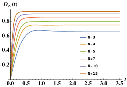
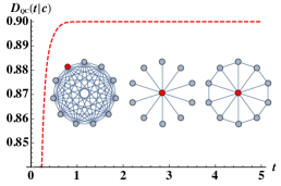
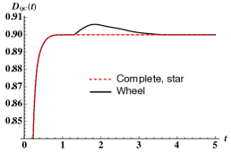
Figure 1: Left panel: QC-distance for complete graphs of different sizes $N$. Central panel: the quantity $\hbox{D}_{\hbox{\tiny QC}}(t|c)$ for the complete, star and wheel graphs, starting from the initial central site $\ket{c}$, depicted in red in the insets. Right panel: QC-distance for the graphs of the central panel.

III Universal properties of the QC-distance

As already mentioned above, the QC-distance $\hbox{D}_{\hbox{\tiny QC}}(t)$ is a positive quantity bounded between 0 and 1. Since we know from theorem 1 that the optimal initial state achieving the maximum in (3) is a localized state $\rho_{j}$, let us analyze the temporal behavior and properties of the fidelity

$$\mathcal{F}_{j}(t)=\sum_{k}p_{kj}(t)|\alpha_{kj}(t)|^{2}$$ (6)

for a walker initially localized on the node $j$. This expression allows us to explore the behavior of the conditional distances $\hbox{D}_{\hbox{\tiny QC}}(t|j)=1-\mathcal{F}_{j}(t)$ in different regimes. In particular, in the short-time limit $t\ll 1$, we find that $\hbox{D}_{\hbox{\tiny QC}}(t|j)$ depends only on the degree of the corresponding node, i.e. $d_{j}=-\bra{j}L\ket{j}$, as follows

$$\hbox{D}_{\hbox{\tiny QC}}(t\ll 1|j)=d_{j}t+O(t^{2})\,.$$ (7)

This result is obtained by expanding the transition probabilities $p_{kj}(t)$ and the tunneling amplitudes $\alpha_{kj}(t)$ up to first order in time

$$p_{kj}(t) =\delta_{kj}+t\matrixelement{k}{L}{j}+O(t^{2})$$ (8)

$$\alpha_{kj}(t) =\delta_{kj}+it\matrixelement{k}{L}{j}+O(t^{2})\,,$$ (9)

and then substituting these expression in $\mathcal{F}_{j}(t)$, with the reminder that the off-diagonal elements of $L$ are positive, while the diagonal ones are negative. The meaning of Eq. (7) is that the more connected the initial node is, the larger is the difference betweeen the dynamics of a QW and a RW on the given graph. The QC-distance $\hbox{D}_{\hbox{\tiny QC}}(t)=\max_{j}\hbox{D}_{\hbox{\tiny QC}}(t|j)$ for a given graph is thus determined by the vertex with maximum degree.

Concerning the behaviour for large times, we notice that for a classical walker the distribution over the nodes tends to the flat distribution, i.e. for $t\gg 1$ we have $\mathcal{E}_{\textsc{c}}(\rho_{\textsc{c}})=\mathbb{I}/N$, $\forall\rho_{\textsc{c}}$. In turn, we have $\mathcal{F}_{j}=1/N$, $\forall j$ and therefore we can rewrite the QC-distance in the long-time regime as

$$\hbox{D}_{\hbox{\tiny QC}}(t\gg 1)\simeq 1-\frac{1}{N}\,,$$ (10)

independently on the topology of the graph.

The physical interpretation of the above results is rather clear: at short times what really matters is the connecttivity of the initial node. This is a local phenomenon and does not depend on the dimension of the graph. As time passes, classical and quantum walkers evolve, and explore the whole graph until the CT-RW achieves the stationary uniform distribution over the graph, while the CT-QW periodically evolves both in populations and coherences. This leads to a stationary value for the QC-distance, depending only on the size of the graph, which is a global property. This is illustrated in the left panel of Fig. 1, where we display, as an example, the behavior of the QC-distance as a function of time for complete graphs of different sizes. The initial slope of the curves at short times is the vertex degree, while at long times the stationary value $1-1/N$ is reached.

The intermediate-time behavior of $\hbox{D}_{\hbox{\tiny QC}}(t)$ is related to the topology of the graph, with the main contribution coming from its algebraic connectivity. In order to see this, we notice that the squared amplitudes $|\alpha_{kj}(t)|^{2}$ are bounded (and oscillating) functions, whereas the classical transition probabilities may be written as

$$p_{kj}(t) =\sum_{s=0}^{N}e^{-|\lambda_{s}|t}\langle k|\lambda_{s}\rangle\langle\lambda_{s}|j\rangle$$

$$=\delta_{kj}+\sum_{s=1}^{N}e^{-|\lambda_{s}|t}\langle k|\lambda_{s}\rangle\langle\lambda_{s}|j\rangle\,,$$ (11)

where we have introduced the eigenvalues and eigenvectors of the Laplacian $L=\sum_{s}\lambda_{s}|\lambda_{s}\rangle\langle\lambda_{s}|$ and already took into account that the smallest (in modulus) eigenvalue of a Laplacian is always zero. The dominant term in $p_{kj}(t)$ and, in turn, in the fidelity, is thus the one containing $|\lambda_{1}|$, which is usually referred to as the Fiedler value or Fiedler eigenvalue of the Laplacian, providing an overall algebraic quantification of the connectivity of the graph fiedler .

IV Graph-dependent properties of the QC-distance

The definition of the QC-distance involves a maximization over the initial state of the walker. There may be, however, situations where the $\hbox{D}_{\hbox{\tiny QC}}(t|j)$ themselves may be of interest, e.g. when there exists a privileged node to start with, and we want to assess the effect of different topologies. This kind of situation is illustrated in the central and right panels of Fig. 1, where we compare the behavior of $\hbox{D}_{\hbox{\tiny QC}}(t|c)$ for the complete, star and wheel graphs, $\ket{c}$ being the central node (see the red points in the inset). As shown in the central panel, $\hbox{D}_{\hbox{\tiny QC}}(t|c)$ is the same for all graphs, since they all have a central node $\ket{c}$ with degree $N-1$ and there is at least a localized preparation on all graphs leading to the same dynamics. On the other hand, if we look at the QC-distance $\hbox{D}_{\hbox{\tiny QC}}(t)$, we see that for the wheel graph it departs from the others curves in a certain time interval. In fact, it increases linearly at short times according to Eq. (7), whereas, as time grows, the proportionality is lost and the topology of the graph plays a role in the behavior of the NC. This is physically consistent, since $\hbox{D}_{\hbox{\tiny QC}}(t)$ distance aims to quantify a property of the graph itself rather than the properties of specific preparations.

Let us illustrate this behaviour with a different example, i.e. we consider different graphs with a fixed size, say $N=11$, and different connectivity. In particular, we start by consider a a ring graph, where all the nodes have degree equal to two and then select one node, e.g. $\ket{1}$ and take random connected graphs with increasing number of links, i.e. we increase the node degree $d_{1}$. The behaviour of $\hbox{D}_{\hbox{\tiny QC}}(t|1)$ is shown in Fig. 2. At short times, the ring graph has the lowest value of $\hbox{D}_{\hbox{\tiny QC}}(t|1)$, but then it shows a maximum value in time, which is higher compared to the other graphs. In other words, the evolution of a quantum walker on a ring graph is initially closer to its classical counterpart compared to other graphs with larger $d_{1}$, but then, for larger times, it becomes more nonclassical, i.e. it departs more from the classical dynamics compared to the other considered graphs. The insets show some of the considered graphs with degrees $d_{1}=2,6,10$, respectively.

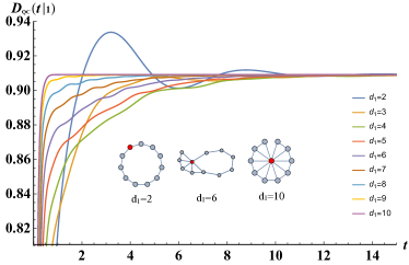
Figure 2: The distance $\hbox{D}_{\hbox{\tiny QC}}(t|1)$ for different graphs having the same size $N=11$ and different degree of node $1$. The blue oscillating line denotes $\hbox{D}_{\hbox{\tiny QC}}(t|1)$ for the ring graph. The insets show some of the considered graphs with degrees $d_{1}=2,6,10$ respectively. The plot shows that for short times the ring graph has the lowest value of $\hbox{D}_{\hbox{\tiny QC}}(t|1)$, whereas at later times its $\hbox{D}_{\hbox{\tiny QC}}(t|1)$ is larger than those of the other graphs, i.e. it departs more from the classical dynamics.

Depending on the application at hand, one may be also interested in assessing the average dynamics over a graph. To this aim, let us also briefly discuss another notion of QC-distance, taking into account the role of different initial positions. This is the average of $\hbox{D}_{\hbox{\tiny QC}}(t|j)$ over the localized states, i.e.

$$\overline{\hbox{D}}_{\hbox{\tiny QC}}(t)=\frac{1}{N}\sum_{k=1}^{N}\hbox{D}_{\hbox{\tiny QC}}(t|j),$$ (12)

which may be naturally referred to as the average QC-distance. For regular graphs, it coincides with $\hbox{D}_{\hbox{\tiny QC}}(t)$, whereas for non-regular graphs it accounts for the fact that a walker initially localized on different nodes may evolve very differently. The behaviour of $\overline{\hbox{D}}_{\hbox{\tiny QC}}(t)$ may be easily recovered from the previous analysis. We have ${\overline{\hbox{D}}_{\hbox{\tiny QC}}}(t\gg 1)\simeq\overline{d}\,t$ for short times, where $\overline{d}$ is the average degree of the graph and ${\overline{\hbox{D}}_{\hbox{\tiny QC}}}(t)(t\gg 1)\simeq 1-\frac{1}{N}$ for long times.

   

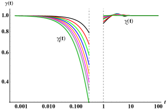
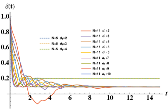
Figure 3: Left panel: the ratios $\gamma_{\text{\tiny S}}(t)$ and $\gamma_{\text{\tiny L}}(t)$ between the exact QC-distance and its asymptotic expressions derived from (LABEL:final_cfr) for short and long times for several graphs of size $N=11$. The plot illustrates the fact that the range of validity of the short time expression $\hbox{D}_{\hbox{\tiny QC}}^{\text{\tiny S}}(t|j)$ depends quite strongly on the kind of graph, whereas the convergence to the asymptotic value $\hbox{D}_{\hbox{\tiny QC}}^{\text{\tiny L}}(t)=1-1/N$ is almost independent on the graph, and it is achieved quite rapidly. Right panel: the difference $\delta(t)$ between the classical distance and the renormalized coherence for the several graphs of size $N=11$ and $N=5$. Here the convergence time increases with the size of the graph, still being independent on its topology.

V The role of coherence and classical fidelity

The QC-distance quantifies how much the evolution of a quantum walker on a graph differs from its CT-RW counterpart. A question arises on whether this difference is due to the appearance of genuine quantum features, or it is just due to differences in the two maps $\mathcal{E}_{\textsc{c}}$ and $\mathcal{E}_{\textsc{q}}$. As we will see the answer is not trivial and time-dependent. Let us briefly recall the notion of coherence of a quantum state, a genuine quantum property with no classical analogue. Coherence may be properly quantified by the sum of the off-diagonal elements of the density matrix, i.e. plenio14 $C(t)\equiv\sum_{k\neq j}\absolutevalue{\rho_{kj}(t)}$. For the dynamics of a quantum walker the natural basis to consider is that of localized states. The coherence at time $t$ is thus given by

$$C_{j}(t)=\left(\sum_{k}\absolutevalue{\alpha_{kj}(t)}\right)^{2}-1,$$ (13)

where the index $j$ refers to the localized initial state of the quantum walker. By construction, any classical state of the form (1) has zero coherence, i.e. it is incoherent. By expanding this expression for short times, up to first order, and comparing it with the expression of nonclassicality in Eq. (7) we find

$$\hbox{D}_{\hbox{\tiny QC}}(t\ll 1|j)=\frac{1}{2}C_{j}(t)\,.$$

It follows that the initial behavior of the QC-distance at short times is governed solely by the amount of coherence created by the dynamics. In other words, the difference in the dynamics may be fully attributed to the appearance of genuine quantum features. On the other hand, this is no longer true at later times, where a substantial contribution to $\hbox{D}_{\hbox{\tiny QC}}(t)$ is due to differences in the distribution over sites. In order to prove this statement, let us introduce the classical fidelity between the probability distributions over the sites of CT-RW and CT-QW, i.e.

$$G_{j}(t)=\sum_{k}\sqrt{p_{kj}(t)|\alpha_{kj}(t)|^{2}}\,.$$ (14)

For large times $p_{kj}(t)\simeq 1/N$, and thus we have

$$\sqrt{N}G_{j}(t){\simeq}\sum_{k}|\alpha_{kj}(t)|\,$$

and, in turn,

$$N\,G_{j}^{2}(t)-C_{j}(t){\simeq}1\,.$$

Since for large times $\hbox{D}_{\hbox{\tiny QC}}(t|j)\simeq 1-1/N$, we may summarize the above results as follows

$$\hbox{D}_{\hbox{\tiny QC}}(t|j)=\begin{cases}\hbox{D}_{\hbox{\tiny QC}}^{\text{\tiny S}}(t|j)\equiv\frac{1}{2}\,{C_{j}(t)}&t\ll 1\\ &\\ \hbox{D}_{\hbox{\tiny QC}}^{\text{\tiny L}}(t|j)\equiv 1-G_{j}^{2}(t)+\frac{1}{N}\,{C_{j}(t)}&t\gg 1\end{cases}\,,$$ (15)

from which, after maximizing over nodes, we obtain the asymptotic expression of $\hbox{D}_{\hbox{\tiny QC}}(t)$ in terms of coherence and classical fidelity. Eq. (LABEL:final_cfr) shows that that for short times a nonzero QC-distance may be ascribed to the appearance of coherence, whereas for long times quantum features accounts only partially for the difference between the two dynamics. In this regime, QC-distance is the sum of the normalised coherence and the distance between the probability distributions over the nodes of the graph. We also remark that $\hbox{D}_{\hbox{\tiny QC}}(t)$ no longer depends on the topology of the consider graph, but rather only on its size. In order to assess the generality of this statement, and the range of validity of Eq. (LABEL:final_cfr), we have considered different classes of graphs and evaluated the ratios

$$\gamma_{\text{\tiny K}}(t)=\hbox{D}_{\hbox{\tiny QC}}(t)/\hbox{D}_{\hbox{\tiny QC}}^{\text{\tiny K}}(t)\,\qquad K=S,L\,,$$

between the exact QC-distance (calculated numerically) and its limiting expressions derived from Eq. (LABEL:final_cfr) for short and long times. In the left panel of Fig. 3 we report the two values of $\gamma$ for a set of random graphs of size $N=11$. As it is apparent from the plot, the range of validity of the short time expression $\hbox{D}_{\hbox{\tiny QC}}^{\text{\tiny S}}(t|j)$ depends quite strongly on the kind of graph, whereas the convergence to the asymptotic value $\hbox{D}_{\hbox{\tiny QC}}^{\text{\tiny L}}(t)=1-1/N$ is almost independent on the graph, and it is achieved quite rapidly. The same rapid convergence to the value $\delta(t)=1/N$ may be seen for the difference $\delta(t)=G^{2}(t)-C(t)/N$ between the square of the classical fidelity and the size-normalized coherence (see the right panel of Fig. 3). Here the convergence time increases with the size of the graph, still being independent on its topology.

VI Discussion and conclusions

We have introduced a fidelity-based measure, termed QC-distance $\hbox{D}_{\hbox{\tiny QC}}(t)$, to properly compare the dynamical behaviour of classical and quantum walks over a graph, also discussing the role of size and topology of the graph. Our results show that at short times, the QC-distance of quantum walks is proportional to the local connectivity, and in turn to coherence, i.e. to the appearance of a genuine quantum feature. On the other hand, in the long time limit, quantumness plays only a partial role, since the QC-distance is the sum of a size-normalised measure of coherence and the classical distance between the probability distributions over the graph. The graph topology is not relevant in those two limiting regimes, whereas it plays a role in determining the QC-distance at intermediate times. Notice that the two terms in $\hbox{D}_{\hbox{\tiny QC}}^{L}(t)$ are approximately of the same magnitude, i.e. coherence and classical distance contribute almost equally to the QC-distance.

From the physical point of view, the behavior of $\hbox{D}_{\hbox{\tiny QC}}(t)$ tells us that the difference between CT-RW and CT-QW may be initially ascribed to the ability of a quantum walker to tunnel between sites, whereas for longer times coherence cannot fully account for the difference in the dynamics. In this regime, QC-distance is also due to the periodic nature of CT-QW dynamics, compared to the diffusive one of CT-RW, which leads to an equilibrium state. In other words, the differences in the long times dynamics should be equally ascribed to the appearance of quantum features, as well as to the different nature (open vs closed system) of the two dynamical models.

We put forward our measure as a tool in assessing the role of quantum features in the dynamics of quantum complex networks and in the design of quantum protocols over graphs. We also believe that it paves the way to define the nature and the amount of quantumness in many particle quantum walks.

References

- (1) S. E. Venegas-Andraca, Quantum walks: a comprehensive review, Quantum Inf. Process. 11, 1015 (2012).
- (2) O. Mülken and A. Blumen, Continuous-Time Quantum Walks: Models for Coherent Transport on Complex Networks, Phys. Rep. 502, 37 (2011).
- (3) A. Ambainis, quantum walks and their algorithmic applications, Int. J. Quantum Inf. 1, 507 (2003).
- (4) A. M. Childs, Universal Computation by Quantum Walk, Phys. Rev. Lett. 102, 180501 (2009).
- (5) E. Farhi and S. Gutmann, Analog analogue of a digital quantum computation, Phys. Rev. A 57, 2403 (1998).
- (6) A. Ambainis, Quantum Walk Algorithm for Element Distinctness, SIAM J. Comput. 37, 210 (2007).
- (7) A. M. Childs, J. Goldstone, Spatial search by quantum walk, Phys. Rev. A 70, 022314 (2004).
- (8) D. Tamascelli and L. Zanetti, A quantum-walk-inspired adiabatic algorithm for solving graph isomorphism problems, J. Phys. A 47, 325302 (2014).
- (9) A. M. Childs, E. Farhi and S. Gutmann, Quantum Inf. Proc., 1, 35 (2002).
- (10) N. Konno, Limit theorem for continuous-time quantum walk on the line, Phys. Rev. E 72, 026113 (2005).
- (11) M. Faccin, T. Johnson, J. Biamonte, S. Kais, and P. Migdał, Degree Distribution in Quantum Walks on Complex Networks, Phys. Rev. X 3, 041007 (2013).
- (12) F. Shahbeigi, S. J. Akhtarshenas, A. T. Rezakhani, How Quantum is a Quantum Walk, arXiv:1802.07027
- (13) B. E. Szigeti, G. Homa, Z. Zimborás, N. Barankai, Short time behavior of continuous time quantum walks on graphs, Phys. Rev. A 100, 062320 (2019)
- (14) T. Kopyciuk, M. Lewandowski, P. Kurzynski, re- and post-selection paradoxes in quantum walks, arXiv:1905.13501
- (15) O. Mülken and A. Blumen, Spacetime structures of continuous-time quantum walks, Phys. Rev. E 71, 036128 (2005).
- (16) Balaji R. Rao, R. Srikanth, C. M. Chandrashekar, and S. Banerjee, Quantumness of noisy quantum walks: A comparison between measurement-induced disturbance and quantum discord, Phys. Rev. A 83, 064302 (2011).
- (17) C. Benedetti, F. Buscemi, P. Bordone, M. G. A. Paris, Non-Markovian continuous-time quantum walks on lattices with dynamical noise, Phys. Rev. A 93, 042313 (2016).
- (18) C. Benedetti, M. A. C. Rossi, M. G. A. Paris, Continuous-time quantum walks on dynamical percolation graphs, EPL 124, 60001 (2018).
- (19) E. Farhi and S. Gutmann, Quantum computation and decision trees, Phys. Rev. A 58, 915 (1998).
- (20) T. G. Wong, L. Tarrataca, and N. Nahimov, Quantum Inf. Process. 15, 4029 (2016).
- (21) M. Newman, Networks: An Introduction (Oxford University Press, 2010).
- (22) R. Jozsa , Fidelity for Mixed Quantum States, J. Mod. Opt. 41, 2315 (1994).
- (23) M. Raginsky, A fidelity measure for quantum channels, Phys. Lett. A 290, 11 (2001).
- (24) A. Gilchrist, N. K. Langford, M. A. Nielsen, Distance measures to compare real and ideal quantum processes, Phys. Rev. A 71, 062310 (2005).
- (25) H.B. Chen, C. Gneiting, P.-Y. Lo, Y.-N. Chen, F. Nori, Simulating open quantum systems with hamiltonian ensembles and the nonclassicality of the dynamics, Phys. Rev. Lett. 120, 030403 (2018).
- (26) A. Uhlmann, Simultaneous decompositions of two states , Rep. Math. Phys. 45, 407 (2000).
- (27) M. Fiedler, Algebraic connectivity of graphs, Czechoslovak Math. J. 23, 298 (1973).
- (28) T. Baumgratz, M. Cramer, and M. B. Plenio, Quantifying Coherence, Phys. Rev. Lett. 113, 140401 (2014).