An efficient numerical scheme for a 3D spherical dynamo equation

Abstract

We develop an efficient numerical scheme for the 3D mean-field spherical dynamo equation. The scheme is based on a semi-implicit discretization in time and a spectral method in space based on the divergence-free spherical harmonic functions. A special semi-implicit approach is proposed such that at each time step one only needs to solve a linear system with constant coefficients. Then, using expansion in divergence-free spherical harmonic functions in the transverse directions allows us to reduce the linear system at each time step to a sequence of one-dimensional equations in the radial direction, which can then be efficiently solved by using a spectral-element method. We show that the solution of fully discretized scheme remains bounded independent of the number of unknowns, and present numerical results to validate our scheme.

Keywords and phrases: spherical dynamo model, vector spherical harmonics, spectral method, stability, convergence.

AMS subject classifications: 65M12, 65M70, 41A30, 86-08

1 Introduction

It is well known that many astrophysical bodies have intrinsic magnetic fields. For examples, Earth possesses a magnetic field that has been known for many centuries; sunspots is the best-known manifestation of the solar magnetic activity cycle. But only in the last few decades scientists began to try to understand more about the origin of these magnetic fields. It is widely accepted that the magnetic activities of many planets and stars represent the magnetohydrodynamic dynamo processes taking place in their deep interiors. For the physical background of the dynamo model, we refer to R. Hollerbach [9] or Chris A. Jones [11] and the references therein.

There are numerous simplified mathematical models and numerical simulations in the literature (see, e.g. Bullard et al. [3], R. Hollerbach[10], R. A. Bayliss, et al. [2], C. Guervilly, and P. Cardin, [7], Chris A. Jones [11], W. Kuang and J. Bloxham [13], David Moss [14], K. Zhang and F. Buss [24] Paul H. Roberts, et al., [19] and the references therein). There are also a few studies with numerical analysis on some numerical methods for these models, e.g.,[4], [17], [23], [5] and [18]. In [4], Chan, Zhang and Zou studied the mathematical theory and its numerical approximation based on a finite element method, while Mohammad M. Rahman and David R. Fearn [18] developed a spectral approximation of some nonlinear mean-field dynamo equations with different geometries and toroidal and poloidal decomposition.

There are two main difficulties in dealing with dynamo models: (i) it consists of three-dimensional vector equations in spherical shells; and (ii) the magnetic field is implicitly divergence-free. Using a finite-element method to deal with the above issues may be complicated and costly. We consider in this paper the model used in [4] and propose an efficient numerical scheme based on a semi-implicit discretization in time and a spectral method in space based on the divergence-free spherical harmonic functions. we first discretize the model in time using a semi-implicit approach such that at each time step one only needs to solve a linear system with piecewise constant coefficients. Then, we discretize this linear system by using a spectral discretization consisting of divergence-free spherical harmonic functions in the transverse directions and a spectral-element method in the radial direction. This way, the linear system can be reduced to a sequence of one-dimensional equations in the radial direction for the coefficients of the expansion in divergence-free spherical harmonic functions so that it can be efficiently and accurately solved by using a spectral-element method.

The remainder of this paper is organized as follows. In section 2, we describe the model that we consider, list some of its mathematical properties, and some useful mathematical tools that will be used later. In Section 3, a fully discrete spectral method for approximating the continuous problem is proposed. The stability and the convergence analysis of our numerical solutions are carried out in section 4. Section 5 contains implementation details, and a numerical experiment is shown in section 6 that demonstrates the efficiency of our numerical scheme.

2 Preliminaries

2.1 The Model

We consider the following nonlinear spherical mean-field dynamo system:

$$\left\{\begin{array}[]{lll}&\boldsymbol{b}_{t}+\nabla\times(\beta(\boldsymbol{x})\nabla\times\boldsymbol{b})=R_{\alpha}\nabla\times(\frac{f(x,t)}{1+\sigma|\boldsymbol{b}|^{2}}\boldsymbol{b})+R_{m}\nabla\times(\boldsymbol{u}\times\boldsymbol{b})&\mbox{in}\ \ \Omega\times(0,T),\\ &\nabla\times\boldsymbol{b}\times\mathbf{n}=0&\mbox{on}\ \ {\partial\Omega\times(0,T)},\\ &\boldsymbol{b}(\boldsymbol{x},0)=\boldsymbol{b}^{0}(\boldsymbol{x})&\mbox{in}\ \ \Omega.\end{array}\right.$$ (2.1)

Figure 1: Domain $\Omega$

The unknown is the magnetic field $\boldsymbol{b}$. $\Omega$ is the physical domain of interest, which consists of three non-overlapping zones $\Omega_{k}\,(k=1,2,3)$ in spherical geometry (see Figure 1), where $\Omega_{1}$ is the core, $\Omega_{2}$ is the convection zone and $\Omega_{3}$ is the outer photosphere. $\mathbf{n}$ denotes the unit outer normal vector to the boundary of $\Omega$. The physical meanings of the variables in (2.1) are as follows: $\boldsymbol{u}=\boldsymbol{u}(\boldsymbol{x},t)$ represents the fluid velocity field, which is given here, and $f(\boldsymbol{x},t)$ is also a known function. Both $\boldsymbol{u}$ and $f$ vanish on $\bar{\Omega}_{1}$ and $\bar{\Omega}_{3}$. The non-dimensional parameters $R_{\alpha},\ R_{m}$ are Rayleigh numbers, $\sigma$ is a constant, $\beta(\boldsymbol{x})$ is the magnetic diffusivity satisfying $\beta_{1}\leq\beta(\boldsymbol{x})\leq\beta_{2}$. The diffusivity is considered as constant in the convection zone. At the two interfaces $\Gamma_{1}$ and $\Gamma_{2}$, we impose the physical jump conditions

$$[\beta(\boldsymbol{x})\nabla\times\boldsymbol{b}\times\mathbf{n}]=0,\ [\boldsymbol{b}]=0\ \ \ \ \mbox{on}\ (\Gamma_{1}\cup\Gamma_{2})\times(0,T),$$ (2.2)

where $[\boldsymbol{a}]$ denotes the jumps of $\boldsymbol{a}$ across the interfaces and $\mathbf{n}$ is the outward normal.

Remark 2.1.

Taking the divergence of the first equation in (2.1), we find $\text{div}{\boldsymbol{b}}_{t}=0$. Hence, if we impose the condition $\nabla\cdot\boldsymbol{b}^{0}=0$, we have $\nabla\cdot\boldsymbol{b}=0\ \mbox{in}\ \ \Omega\times(0,T)$.

We now describe some notations, and recall some basic mathematical properties for (2.1). We denote by $H^{m}(\Omega)\,(m\in\mathbb{R})$ the usual Sobolev space, and denote $H^{m}(\Omega)^{3}$ by $\boldsymbol{H}^{m}(\Omega)$. As usual, $(\cdot,\cdot)$ denotes the scalar product in $\boldsymbol{L}^{2}(\Omega)$ or $L^{2}(\Omega)$. For real $s\geq 0$, $\|\cdot\|_{s}$ denotes the norm of $\boldsymbol{H}^{s}(\Omega)$ (or the $H^{s}(\Omega)$ for scalar functions), in particular, we denote $\|\cdot\|_{0}\triangleq\|\cdot\|.$ We define

$${\boldsymbol{V}}=\{\boldsymbol{c}\in\boldsymbol{L}^{2}(\Omega);\mathbf{curl}\ \boldsymbol{c}\in\boldsymbol{L}^{2}(\Omega)\},$$

and for all $\ \boldsymbol{c}\in{\boldsymbol{V}},$ we set

$$\|\boldsymbol{c}\|_{\boldsymbol{V}}^{2}=\|\boldsymbol{c}\|^{2}+\|\nabla\times\boldsymbol{c}\|^{2}.$$

We consider the following weak formulation for (2.1):

Find $\boldsymbol{b}(t)\in{\boldsymbol{V}}$ such that $\boldsymbol{b}(0)=\boldsymbol{b}_{0}$ and for almost all $t\in(0,T),$

$$(\boldsymbol{b}^{\prime}(t),\boldsymbol{a})+(\beta\nabla\times\boldsymbol{b}(t),\nabla\times\boldsymbol{a})$$ (2.3)

$$= R_{\alpha}\left(\frac{f(t)}{1+\sigma|\boldsymbol{b}|^{2}}\boldsymbol{b}(t),\nabla\times\boldsymbol{a}\right)+R_{m}(\boldsymbol{u}(t)\times\boldsymbol{b}(t),\nabla\times\boldsymbol{a}),\hskip 22.76228pt\forall\ \boldsymbol{a}\in{\boldsymbol{V}}.$$

By using a standard argument (cf. M. Sermange and R. Temam [20]), one can easily derive the following result:

Theorem 2.1.

There exists a unique solution $\boldsymbol{b}$ to the dynamo system (2.3) such that

$$\boldsymbol{b}\in L^{\infty}(0,T;\boldsymbol{V})\cap H^{1}(0,T;\boldsymbol{L}^{2}(\Omega))$$

provided that $\boldsymbol{b}_{0}\in{\boldsymbol{V}},\ f\in H^{1}(0,T;L^{\infty}(\Omega)),\ \boldsymbol{u}\in H^{1}(0,T;\boldsymbol{L}^{\infty}(\Omega))$. More precisely, there exists a constant $C>0$ such that

$$\|\boldsymbol{b}\|^{2}_{L^{\infty}(0,T;\boldsymbol{V})}+\|\boldsymbol{b}\|^{2}_{H^{1}(0,T;\boldsymbol{L}^{2}(\Omega))}$$ (2.4)

$$\leq C\left(\|\nabla\times\boldsymbol{b}^{0}\|^{2}+\|\boldsymbol{b}^{0}\|^{2}\right)\max\limits_{0\leq t\leq T}\left(\|f(t)\|_{L^{\infty}(\Omega)}^{2}+\|\boldsymbol{u}(t)\|_{\boldsymbol{L}^{\infty}(\Omega)}^{2}\right)$$

$$\cdot\exp\left(C\displaystyle\int_{0}^{T}{\|f(t)\|_{L^{\infty}(\Omega)}^{2}+\|f^{\prime}(t)\|_{L^{\infty}(\Omega)}^{2}+\|\boldsymbol{u}(t)\|_{\boldsymbol{L}^{\infty}(\Omega)}^{2}+\|\boldsymbol{u}^{\prime}(t)\|_{\boldsymbol{L}^{\infty}(\Omega)}^{2}}\right).$$

2.2 Some Useful Mathematical Tools

We recall below some lemmas which will be used later.

Lemma 2.2.

(Young’s inequality) For any $a,b\in\mathbb{R}$ and $\varepsilon>0$, we have

$$ab\leq\varepsilon a^{2}+\frac{1}{4\varepsilon}b^{2}.$$

Lemma 2.3.

(Discrete integration by parts) Let $\{\boldsymbol{a}_{n}\}_{n=0}^{k}$ and $\{\boldsymbol{b}_{n}\}_{n=1}^{k}$ be two vector sequences, then we have

$$\sum\limits_{n=1}^{k}(\boldsymbol{a}_{n}-\boldsymbol{a}_{n-1})\cdot\boldsymbol{b}_{n}=\boldsymbol{a}_{k}\cdot\boldsymbol{b}_{k}-\boldsymbol{a}_{0}\cdot\boldsymbol{b}_{1}-\sum\limits_{n=1}^{k-1}\boldsymbol{a}_{n}\cdot(\boldsymbol{b}_{n+1}-\boldsymbol{b}_{n}).$$

Proof.

By direct calculation, we easily get

$$\sum\limits_{n=1}^{k}({a}_{n}-{a}_{n-1})\cdot{b}_{n}={a}_{k}\cdot{b}_{k}-{a}_{0}\cdot{b}_{1}-\sum\limits_{n=1}^{k-1}{a}_{n}\cdot({b}_{n+1}-{b}_{n})$$

for scalar sequences $\{{a}_{n}\}_{n=0}^{k}$ and $\{{b}_{n}\}_{n=1}^{k}$. The desired result for vector sequences can be obtained accordingly. ∎

Lemma 2.4.

(Gronwall inequality) Let $f\in L^{1}(t_{0},T)$ be a non-negative function, $g$ and $\phi$ be continuous functions on $[t_{0},T]$. Moreover $g$ is non-decreasing. Then

$$\phi(t)\leq g(t)+\int_{t_{0}}^{t}f(\tau)\phi(\tau)\,d\tau\ \ \ \forall\ t\in[t_{0},T]$$

implies that

$$\phi(t)\leq g(t)e^{\int_{t_{0}}^{t}f(\tau)\,d\tau}\ \ \ \forall\ t\in[t_{0},T].$$

Remark 2.2.

We will frequently use the following special case:

$$f(t)\leq C+\alpha\displaystyle\int_{0}^{t}f(s)ds\ \ \ \ \mbox{\rm implies that}\ \ f(t)\leq Ce^{\alpha t}\ \ \ \forall\ t\in[0,T],$$ (2.5)

where $\alpha\geq 0$ and $C$ are given constants.

Lemma 2.5.

([6], p.34) (Integration by parts) Let $\Omega$ be a bounded region of $\mathbb{R}^{d}$ ($d=2$ or 3) with Lipschitz continuous boundary. Then, the mapping

$$\gamma_{\tau}:\left\{\begin{array}[]{ll}\boldsymbol{v}\to\boldsymbol{v}\cdot\tau|_{\partial\Omega}&\ {\rm for}\ \ d=2,\\ \boldsymbol{v}\to\boldsymbol{v}\times\mathbf{n}|_{\partial\Omega}&\ {\rm for}\ \ d=3\end{array}\right.$$

can be extended by continuity to a linear and continuous mapping, still denoted by $\gamma_{\tau}$, from $\boldsymbol{V}$ into $H^{-1/2}(\partial\Omega)$ if $d=2$ or $H^{-1/2}(\partial\Omega)^{3}$ if $d=3$, where $\tau$ is the unit tangent vector to $\partial\Omega$. Furthermore, the following Green’s formula holds:

$$(\nabla\times\boldsymbol{v},\boldsymbol{\phi})=(\boldsymbol{v},\nabla\times\boldsymbol{\phi})-\langle\gamma_{\tau}\boldsymbol{v},\boldsymbol{\phi}\rangle_{\partial\Omega}$$ (2.6)

$\forall\ \boldsymbol{v}\in\boldsymbol{V},\forall\ \boldsymbol{\phi}\in H^{1}(\Omega)^{3}\ {\rm if}\ d=3\ {\rm or}\ \phi\in H^{1}(\Omega)\ {\rm if}\ d=2.$

3 The Numerical Scheme

3.1 Time Discretization

We consider uniform grid on the temporal scale $[0,T]$ with $\tau=\displaystyle\frac{T}{K}$, and $t_{i}=i\tau$:

$$0=t_{0}<t_{1}<\cdots<t_{K}=T$$ (3.1)

Define $u^{n}=u(\cdot,t_{n})$ for $0\leq n\leq K$. For a given sequence $\{u^{n}\}_{n=0}^{K}\subset L^{2}(\Omega)$, we apply first order approximation via difference quotient and define the averaging term $\bar{u}^{n}$ as follows:

$$\partial_{\tau}u^{n}=\frac{u^{n}-u^{n-1}}{\tau},\ \ \ \bar{u}^{n}=\frac{1}{\tau}\int_{t_{n-1}}^{t_{n}}u(\cdot,t)dt,\quad 1\leq n\leq K,$$ (3.2)

and we set $\bar{u}^{0}=u(\cdot,0).$

In terms of time discretization, we consider the following semi-implicit scheme. For $n=1,2,\cdots,K$, find $\boldsymbol{b}^{n}$ such that satisfies this differential equation

$$\begin{split}\partial_{\tau}\boldsymbol{b}^{n}&+\nabla\times(\bar{\beta}\nabla\times\boldsymbol{b}^{n})=\nabla\times(\bar{\beta}-\beta(x))\nabla\times\boldsymbol{b}^{n-1}\\ &+R_{\alpha}\nabla\times(\frac{\bar{f}^{n}}{1+\sigma|\boldsymbol{b}_{\boldsymbol{N}}^{n-1}|^{2}}\boldsymbol{b}^{n-1})+R_{m}\nabla\times(\bar{\boldsymbol{u}}^{n}\times\boldsymbol{b}^{n-1}),\end{split}$$ (3.3)

and the boundary conditions

$$\begin{split}&\nabla\times\boldsymbol{b}^{n}\times\mathbf{n}=0,\quad\mbox{on}\quad{\partial\Omega},\\ &[\bar{\beta}\nabla\times\boldsymbol{b}^{n}\times\mathbf{n}]=[(\bar{\beta}-\beta(x))\nabla\times\boldsymbol{b}^{n-1}\times\mathbf{n}],\ [\boldsymbol{b}^{n}]=0\ \ \ \ \mbox{on}\;\;\Gamma_{1}\cup\Gamma_{2}.\end{split}$$ (3.4)

where

$$\bar{\beta}=\left\{\begin{array}[]{ll}\bar{\beta}_{1}\triangleq\max\limits_{x\in\Omega_{1}}\beta,&x\in\Omega_{1},\\ \bar{\beta}_{2}\triangleq\max\limits_{x\in\Omega_{2}}\beta=\beta,&x\in\Omega_{2},\\ \bar{\beta}_{3}\triangleq\max\limits_{x\in\Omega_{3}}\beta,&x\in\Omega_{3}.\end{array}\right.$$

Remark 3.1.

Taking the divergence of (3.3), we find $\partial_{\tau}\nabla\cdot\boldsymbol{b}^{n}=0$. Hence, $\nabla\cdot\boldsymbol{b}^{0}=0$ implies $\nabla\cdot\boldsymbol{b}^{n}=0$ for all $n\geq 1$.

3.2 Spatial Discretization: Vector Spherical Harmonics(VSH)

For the spatial discretization, we are working with three dimensional variables in spherical region, therefore it is natural to consider basic functions that specifically designed for spherical domain.

Let $S$ be a unit sphere and $(r,\theta,\varphi)$ be the spherical coordinates with the moving (right-handed) coordinate basis

$$\begin{split}&{\boldsymbol{e}}_{r}=\big{(}\sin\theta\cos\varphi,\ \sin\theta\sin\varphi,\cos\theta\big{)},\\ &{\boldsymbol{e}}_{\theta}=\big{(}\cos\theta\cos\varphi,\ \cos\theta\sin\varphi,-\sin\theta\big{)},\\ &{\boldsymbol{e}}_{\varphi}=\big{(}-\sin\varphi,\ \cos\varphi,0\big{)}.\end{split}$$ (3.5)

The tangential gradient is defined as

$$\nabla_{S}=\frac{\partial}{\partial\theta}{\boldsymbol{e}}_{\theta}+\frac{1}{\sin\theta}\frac{\partial}{\partial\varphi}{\boldsymbol{e}}_{\varphi}.$$ (3.6)

The spherical harmonic functions are defined via the associated Legendre polynomials:

$$Y_{l}^{m}(\theta,\varphi)=\sqrt{\frac{2l+1}{4\pi}\frac{(l-m)!}{(l+m)!}}P_{l}^{m}(\cos\theta)e^{im\varphi}.$$

Recall that $\{Y_{l}^{m}\}$ form orthonormal basis functions of $L^{2}(S)$. Now we define the vector spherical harmonic functions (VSH) (see, e.g., [8, 16]), which form an orthogonal basis of ${\boldsymbol{L}}^{2}(S)$.

$$\left\{\begin{split}&{\boldsymbol{T}}_{l}^{m}=\nabla_{S}Y_{l}^{m}\times{\boldsymbol{e}}_{r}=\frac{1}{\sin\theta}\frac{\partial Y_{l}^{m}}{\partial\varphi}{\boldsymbol{e}}_{\theta}-\frac{\partial Y_{l}^{m}}{\partial\theta}{\boldsymbol{e}}_{\varphi},\quad l\geq 1,\;|m|\leq l,\\ &{\boldsymbol{V}}_{l}^{m}=(l+1)Y_{l}^{m}{\boldsymbol{e}}_{r}-\nabla_{S}Y_{l}^{m},\quad l\geq 0,\;|m|\leq l,\\ &{\boldsymbol{W}}_{l}^{m}=lY_{l}^{m}{\boldsymbol{e}}_{r}+\nabla_{S}Y_{l}^{m},\quad l\geq 1,\;|m|\leq l,\end{split}\right.$$ (3.7)

Some additional properties of VSH will be provided in Appendix $A$.

Given the above definitions, for any vector function $\boldsymbol{F}(\theta,\phi)$ defined on the sphere, we can decompose the function using VSH and some constant coefficients $\bar{t}_{l}^{m},\bar{v}_{l}^{m},\bar{w}_{l}^{m}$:

$${\color[rgb]{0,0,0}\boldsymbol{F}(\theta,\varphi)=\sum_{l=0}^{\infty}\sum_{|m|=0}^{l}\Big{[}\bar{t}_{l}^{m}{\boldsymbol{T}}_{l}^{m}(\theta,\varphi)+\bar{v}_{l}^{m}{\boldsymbol{V}}_{l}^{m}(\theta,\varphi)+\bar{w}_{l}^{m}{\boldsymbol{W}}_{l}^{m}(\theta,\varphi)\Big{]}.}$$ (3.8)

Considering functions $\boldsymbol{F}(r,\theta,\varphi)$ defined in the three dimensional ball, since the radii direction and the tangential plane are perpendicular to each other, we can decompose $\boldsymbol{F}$ using coefficient functions:

$$\boldsymbol{F}(r,\theta,\varphi)=\sum_{l=0}^{\infty}\sum_{|m|=0}^{l}\Big{[}t_{l}^{m}(r){\boldsymbol{T}}_{l}^{m}(\theta,\varphi)+v_{l}^{m}(r){\boldsymbol{V}}_{l}^{m}(\theta,\varphi)+w_{l}^{m}(r){\boldsymbol{W}}_{l}^{m}(\theta,\varphi)\Big{]}.$$ (3.9)

3.3 Solenoidal Vector Field

One of the numerical challenge is how to maintain the divergence free property in the discrete case. In the traditionally methods, this usually involves staggered grid [22], Lagrange multiplier [15] and penalty or projection methods [12, 1].

There exists a divergence free (i.e., solenoidal) basis, which have been used mostly in astrophysics [3], that can take care of the divergence free condition automatically on the spherical domain. Only till recently, there have been some research and analysis on this subject [21] in the mathematical circle. The detailed derivation of the divergence free basis can be found in Appendix B.

We can expand any solenoidal vector function $\boldsymbol{B}(r,\theta,\varphi)$ as

$$\boldsymbol{B}(r,\theta,\varphi)=\sum_{l=0}^{\infty}\sum_{|m|=0}^{l}t_{l}^{m}(r){\boldsymbol{T}}_{l}^{m}(\theta,\varphi)+\nabla\times(A_{l}^{m}(r){\boldsymbol{T}}_{l}^{m}(\theta,\varphi))+a_{0}^{0}(r)Y_{0}^{0}{\boldsymbol{e}}_{r}.$$ (3.10)

with $\displaystyle d_{2}^{+}a_{0}^{0}(r)=0$. The term $a_{0}^{0}(r)Y_{0}^{0}{\boldsymbol{e}}_{r}$ will vanish once being applied to a curl operator, so in our problem, we will only consider $a_{0}^{0}(r)=0$.

3.4 Weak formulation of full discretization

We mark three intervals on the radial direction $I_{1}=[0,r_{1}],I_{2}=[r_{1},r_{2}],I_{3}=[r_{2},r_{3}]$, with $r_{1},r_{2},r_{3}$ be the radius of surfaces $\Gamma_{1},\Gamma_{2},\partial\Omega$ respectively. Each $I_{i}(i=1,2,3)$ is considered as an element on the radius. Let $\mathbb{C}_{N}$ be the complex polynomial space of degree at most $N$. We define the spectral-element space in the radial direction $X_{N}$ on $I=\{I_{1}\cup I_{2}\cup I_{3}\}$ by

$$X_{N}=\{u_{N}|_{I_{i}}\in\mathbb{C}_{N}:[u]=0,{\rm i.e.}\;u_{1}(r_{1})=u_{2}(r_{1}),u_{2}(r_{2})=u_{3}(r_{2})\}.$$ (3.11)

Let $Y_{M}$ be the truncated solenoidal vector field. We set ${\boldsymbol{N}}=(N,M)$. For a function $\boldsymbol{b}_{\boldsymbol{N}}\in{\boldsymbol{V}}_{\boldsymbol{N}}:=X_{N}\times Y_{M}$, it can be expanded as

$$\boldsymbol{b}_{\boldsymbol{N}}(r,\theta,\varphi)=\sum_{l=0}^{M}\sum_{|m|=0}^{l}t_{l,m}^{N}(r){\boldsymbol{T}}_{l}^{m}(\theta,\varphi)+\nabla\times(A_{l,m}^{N}(r){\boldsymbol{T}}_{l}^{m}(\theta,\varphi)),$$ (3.12)

with $t_{l,m}^{N}(r),A_{l,m}^{N}(r)\in X_{N}$.

Then, our full discrete scheme is as follows: to find $\boldsymbol{b}_{\boldsymbol{N}}^{n}\in{\boldsymbol{V}}_{\boldsymbol{N}}$ such that

$$\begin{split}\displaystyle&\int_{\Omega}\partial_{\tau}\boldsymbol{b}_{\boldsymbol{N}}^{n}\cdot\boldsymbol{a}_{\boldsymbol{N}}d\boldsymbol{x}+\displaystyle\int_{\Omega}\bar{\beta}(\nabla\times\boldsymbol{b}_{\boldsymbol{N}}^{n})\cdot(\nabla\times\boldsymbol{a}_{\boldsymbol{N}})d\boldsymbol{x}=\displaystyle\int_{\Omega}(\bar{\beta}-\beta(x))(\nabla\times\boldsymbol{b}_{\boldsymbol{N}}^{n-1})\cdot(\nabla\times\boldsymbol{a}_{\boldsymbol{N}})d\boldsymbol{x}\\ &+R_{\alpha}\displaystyle\int_{\Omega}\frac{\bar{f}^{n}}{1+\sigma|\boldsymbol{b}_{\boldsymbol{N}}^{n-1}|^{2}}\boldsymbol{b}_{\boldsymbol{N}}^{n-1}\cdot(\nabla\times\boldsymbol{a}_{\boldsymbol{N}})d\boldsymbol{x}+R_{m}\displaystyle\int_{\Omega}(\bar{\boldsymbol{u}}^{n}\times\boldsymbol{b}_{\boldsymbol{N}}^{n-1})\cdot(\nabla\times\boldsymbol{a}_{\boldsymbol{N}})d\boldsymbol{x},\quad\forall\ \boldsymbol{a}_{\boldsymbol{N}}\in{\boldsymbol{V}}_{\boldsymbol{N}},\\ \end{split}$$ (3.13)

with

$$\begin{split}\ [\boldsymbol{b}_{\boldsymbol{N}}^{n}]=0\ \ \ \ \mbox{on}\ \Gamma_{1}\cup\Gamma_{2}\end{split}$$ (3.14)

for $n=1,2,\cdots,K,$ and with initial condition

$$\boldsymbol{b}_{\boldsymbol{N}}^{0}=\Pi_{\boldsymbol{N}}\boldsymbol{b}_{0}(\boldsymbol{x}),$$ (3.15)

where $\Pi_{\boldsymbol{N}}$ is the projection into the solenoidal vector field.

4 Stability analysis

We show in this section that the solution of the fully discretized scheme remain bounded.

Theorem 4.6.

Let $\boldsymbol{b}_{\boldsymbol{N}}^{n}$ be the solution of the spectral method (3.13)-(3.15). We assume $f\in W^{1,\infty}(0,T;L^{\infty}(\Omega))$ and $\boldsymbol{u}\in W^{1,\infty}(0,T;\boldsymbol{L}^{\infty}(\Omega))$. Then there exists positive constants $C$, independent of $N$, such that the following inequalities hold.

$$\ \ \max\limits_{1\leq n\leq M}\|\boldsymbol{b}_{\boldsymbol{N}}^{n}\|^{2}+\tau\sum\limits_{n=1}^{M}\|\nabla\times\boldsymbol{b}_{\boldsymbol{N}}^{n}\|^{2}\leq C(\|\boldsymbol{b}^{0}_{\boldsymbol{N}}\|_{\boldsymbol{V}}^{2}+\tau\|\nabla\times\boldsymbol{b}^{0}_{\boldsymbol{N}}\|^{2}),$$ (4.1)

$$\ \ \max\limits_{1\leq n\leq M}\|\nabla\times\boldsymbol{b}_{\boldsymbol{N}}^{n}\|^{2}+\tau\sum\limits_{n=1}^{M}\|\partial_{\tau}\boldsymbol{b}_{\boldsymbol{N}}^{n}\|^{2}\leq C\|\boldsymbol{b}^{0}_{\boldsymbol{N}}\|_{\boldsymbol{V}}^{2}.$$ (4.2)

Proof.

Let $0\leq\delta=\max\displaystyle\frac{\bar{\beta}-\beta}{\bar{\beta}}<1$. Taking $\boldsymbol{a}_{\boldsymbol{N}}=2\tau\boldsymbol{b}_{\boldsymbol{N}}^{n}$ in (3.13), using the Cauchy-Schwarz inequality, Young inequality and the regularity assumption on $f$ and ${\boldsymbol{u}}$, we can derive

$$\|\boldsymbol{b}_{\boldsymbol{N}}^{n}\|^{2} - \|\boldsymbol{b}_{\boldsymbol{N}}^{n-1}\|^{2}+\|\boldsymbol{b}_{\boldsymbol{N}}^{n}-\boldsymbol{b}_{\boldsymbol{N}}^{n-1}\|^{2}+2\tau\bar{\beta}\|\nabla\times\boldsymbol{b}_{\boldsymbol{N}}^{n}\|^{2}$$

$$\leq \tau\|\bar{\beta}\nabla\times\boldsymbol{b}_{\boldsymbol{N}}^{n}\|^{2}+\frac{\tau}{\bar{\beta}}\int_{\Omega}(\bar{\beta}-\beta(x))^{2}|\nabla\times\boldsymbol{b}_{\boldsymbol{N}}^{n-1}|^{2}\,d\boldsymbol{x}$$

$$+\frac{\epsilon}{2}\tau\|\bar{\beta}\nabla\times\boldsymbol{b}_{\boldsymbol{N}}^{n}\|^{2}+\frac{2}{\epsilon\bar{\beta}}\tau R^{2}_{\alpha}\int_{\Omega}\left(\frac{\bar{f}^{n}}{1+\sigma|\boldsymbol{b}_{\boldsymbol{N}}^{n-1}|^{2}}\right)^{2}|\boldsymbol{b}_{\boldsymbol{N}}^{n-1}|^{2}\,d\boldsymbol{x}$$

$$+\frac{\epsilon}{2}\tau\|\bar{\beta}\nabla\times\boldsymbol{b}_{\boldsymbol{N}}^{n}\|^{2}+\frac{2}{\epsilon\bar{\beta}}\tau R_{m}^{2}\int_{\Omega}|\bar{\boldsymbol{u}}^{n}\times\boldsymbol{b}^{n-1}_{\boldsymbol{N}}|^{2}\,d\boldsymbol{x}$$

$$\leq \tau\|\bar{\beta}\nabla\times\boldsymbol{b}_{\boldsymbol{N}}^{n}\|^{2}+\tau\delta^{2}\|\bar{\beta}\nabla\times\boldsymbol{b}_{\boldsymbol{N}}^{n-1}\|^{2}+\tau\epsilon\|\bar{\beta}\nabla\times\boldsymbol{b}_{\boldsymbol{N}}^{n}\|^{2}+C\tau\|\boldsymbol{b}_{\boldsymbol{N}}^{n-1}\|^{2},$$

which implies

$$\|\boldsymbol{b}_{\boldsymbol{N}}^{n}\|^{2}-\|\boldsymbol{b}_{\boldsymbol{N}}^{n-1}\|^{2}+\tau(1-\epsilon)\|\bar{\beta}\nabla\times\boldsymbol{b}_{\boldsymbol{N}}^{n}\|^{2}\leq\tau\delta^{2}\|\bar{\beta}\nabla\times\boldsymbol{b}_{\boldsymbol{N}}^{n-1}\|^{2}+C\tau\|\boldsymbol{b}_{\boldsymbol{N}}^{n-1}\|^{2}.$$

Taking $\epsilon$ small enough such that $1-\epsilon\geq\delta^{2}+\epsilon$, i.e., $\epsilon\leq\frac{1}{2}(1-\delta^{2})$, we get

$$\|\boldsymbol{b}_{\boldsymbol{N}}^{n}\|^{2}-\|\boldsymbol{b}_{\boldsymbol{N}}^{n-1}\|^{2}+\tau\epsilon\|\bar{\beta}\nabla\times\boldsymbol{b}_{\boldsymbol{N}}^{n}\|^{2}+\tau\delta^{2}(\|\bar{\beta}\nabla\times\boldsymbol{b}_{\boldsymbol{N}}^{n}\|^{2}-\|\bar{\beta}\nabla\times\boldsymbol{b}_{\boldsymbol{N}}^{n-1}\|^{2})\leq C\tau\|\boldsymbol{b}_{\boldsymbol{N}}^{n-1}\|^{2}.$$

Summing up the above relation for $n$ from $1$ to ${M}$, we arrive at

$$\|\boldsymbol{b}^{M}_{\boldsymbol{N}}\|^{2}+\epsilon\tau\sum_{n=1}^{M}\|\bar{\beta}\nabla\times\boldsymbol{b}_{\boldsymbol{N}}^{n}\|^{2}\leq\|\boldsymbol{b}_{\boldsymbol{N}}^{0}\|^{2}+\tau\delta^{2}\|\bar{\beta}\nabla\times\boldsymbol{b}_{\boldsymbol{N}}^{0}\|^{2}+C\tau\sum_{n=0}^{M-1}\|\boldsymbol{b}_{\boldsymbol{N}}^{n}\|^{2},$$

which can also be written as

$$\|\boldsymbol{b}_{\boldsymbol{N}}^{M}\|^{2}+\tau\sum_{n=1}^{M}\|\nabla\times\boldsymbol{b}_{\boldsymbol{N}}^{n}\|^{2}\leq C(\|\boldsymbol{b}_{\boldsymbol{N}}^{0}\|^{2}+\tau\|\nabla\times\boldsymbol{b}_{\boldsymbol{N}}^{0}\|^{2})+C\tau\sum_{n=0}^{M-1}\|\boldsymbol{b}_{\boldsymbol{N}}^{n}\|^{2}.$$

Applying the discrete Gronwall’s inequality to above inequality, we find

$$\max_{1\leq n\leq M}\|\boldsymbol{b}_{\boldsymbol{N}}^{n}\|^{2}+\tau\sum_{n=1}^{M}\|\nabla\times\boldsymbol{b}_{\boldsymbol{N}}^{n}\|^{2}\leq C(\|\boldsymbol{b}_{\boldsymbol{N}}^{0}\|^{2}+\tau\|\nabla\times\boldsymbol{b}_{\boldsymbol{N}}^{0}\|^{2})\leq C(\|\boldsymbol{b}^{0}_{\boldsymbol{N}}\|_{\boldsymbol{V}}^{2}+\tau\|\nabla\times\boldsymbol{b}^{0}_{\boldsymbol{N}}\|^{2}),$$

which is (4.1).

To prove (4.2), we take $\boldsymbol{a}_{\boldsymbol{N}}=\tau\partial_{\tau}\boldsymbol{b}_{\boldsymbol{N}}^{n}=\boldsymbol{b}_{\boldsymbol{N}}^{n}-\boldsymbol{b}_{\boldsymbol{N}}^{n-1}$ in (3.13) to obtain

$$\tau\|\partial_{\tau}\boldsymbol{b}_{\boldsymbol{N}}^{n}\|^{2} + \displaystyle\int_{\Omega}\bar{\beta}(\nabla\times\boldsymbol{b}_{\boldsymbol{N}}^{n})\cdot\nabla\times(\boldsymbol{b}_{\boldsymbol{N}}^{n}-\boldsymbol{b}_{\boldsymbol{N}}^{n-1})\,d\boldsymbol{x}$$

$$-\displaystyle\int_{\Omega}(\bar{\beta}-\beta)(\nabla\times\boldsymbol{b}_{\boldsymbol{N}}^{n-1})\cdot\nabla\times(\boldsymbol{b}_{\boldsymbol{N}}^{n}-\boldsymbol{b}_{\boldsymbol{N}}^{n-1})\,d\boldsymbol{x}$$

$$= R_{\alpha}\displaystyle\int_{\Omega}\frac{\bar{f}^{n}}{1+\sigma|\boldsymbol{b}_{\boldsymbol{N}}^{n-1}|^{2}}\boldsymbol{b}_{\boldsymbol{N}}^{n-1}\cdot\nabla\times(\boldsymbol{b}_{\boldsymbol{N}}^{n}-\boldsymbol{b}_{\boldsymbol{N}}^{n-1})\,d\boldsymbol{x}$$

$$+R_{m}\displaystyle\int_{\Omega}(\bar{\boldsymbol{u}}^{n}\times\boldsymbol{b}_{\boldsymbol{N}}^{n-1})\cdot\nabla\times(\boldsymbol{b}_{\boldsymbol{N}}^{n}-\boldsymbol{b}_{\boldsymbol{N}}^{n-1})\,d\boldsymbol{x}.$$

We derive from the above that

$$\tau\|\partial_{\tau}\boldsymbol{b}_{\boldsymbol{N}}^{n}\|^{2} + \|\bar{\beta}\nabla\times\boldsymbol{b}_{\boldsymbol{N}}^{n}\|^{2}+\displaystyle\int_{\Omega}(\bar{\beta}-\beta)|\nabla\times\boldsymbol{b}_{\boldsymbol{N}}^{n-1}|^{2}\,d\boldsymbol{x}$$

$$= \displaystyle\int_{\Omega}(2\bar{\beta}-\beta)(\nabla\times\boldsymbol{b}_{\boldsymbol{N}}^{n})\cdot(\nabla\times\boldsymbol{b}_{\boldsymbol{N}}^{n-1})\,d\boldsymbol{x}$$

$$+R_{\alpha}\displaystyle\int_{\Omega}\frac{\bar{f}^{n}}{1+\sigma|\boldsymbol{b}_{\boldsymbol{N}}^{n-1}|^{2}}\boldsymbol{b}_{\boldsymbol{N}}^{n-1}\cdot\nabla\times(\boldsymbol{b}_{\boldsymbol{N}}^{n}-\boldsymbol{b}_{\boldsymbol{N}}^{n-1})\,d\boldsymbol{x}$$

$$+R_{m}\displaystyle\int_{\Omega}(\bar{\boldsymbol{u}}^{n}\times\boldsymbol{b}_{\boldsymbol{N}}^{n-1})\cdot\nabla\times(\boldsymbol{b}_{\boldsymbol{N}}^{n}-\boldsymbol{b}_{\boldsymbol{N}}^{n-1})\,d\boldsymbol{x}$$

$$\leq \frac{1}{2}\displaystyle\int_{\Omega}(2\bar{\beta}-\beta)|\nabla\times\boldsymbol{b}_{\boldsymbol{N}}^{n}|^{2}d\boldsymbol{x}+\frac{1}{2}\displaystyle\int_{\Omega}(2\bar{\beta}-\beta)|\nabla\times\boldsymbol{b}_{\boldsymbol{N}}^{n-1}|^{2}\,d\boldsymbol{x}$$

$$+R_{\alpha}\displaystyle\int_{\Omega}\frac{\bar{f}^{n}}{1+\sigma|\boldsymbol{b}_{\boldsymbol{N}}^{n-1}|^{2}}\boldsymbol{b}_{\boldsymbol{N}}^{n-1}\cdot\nabla\times(\boldsymbol{b}_{\boldsymbol{N}}^{n}-\boldsymbol{b}_{\boldsymbol{N}}^{n-1})\,d\boldsymbol{x}$$

$$+R_{m}\displaystyle\int_{\Omega}(\bar{\boldsymbol{u}}^{n}\times\boldsymbol{b}_{\boldsymbol{N}}^{n-1})\cdot\nabla\times(\boldsymbol{b}_{\boldsymbol{N}}^{n}-\boldsymbol{b}_{\boldsymbol{N}}^{n-1})\,d\boldsymbol{x},$$

which can be rewritten as

$$\tau\|\partial_{\tau}\boldsymbol{b}_{\boldsymbol{N}}^{n}\|^{2} + \displaystyle\int_{\Omega}\frac{\beta}{2}(|\nabla\times\boldsymbol{b}_{\boldsymbol{N}}^{n}|^{2}-|\nabla\times\boldsymbol{b}_{\boldsymbol{N}}^{n-1}|^{2})d\boldsymbol{x}$$

$$\leq R_{\alpha}\displaystyle\int_{\Omega}\frac{\bar{f}^{n}}{1+\sigma|\boldsymbol{b}_{\boldsymbol{N}}^{n-1}|^{2}}\boldsymbol{b}_{\boldsymbol{N}}^{n-1}\cdot\nabla\times(\boldsymbol{b}_{\boldsymbol{N}}^{n}-\boldsymbol{b}_{\boldsymbol{N}}^{n-1})d\boldsymbol{x}$$

$$+R_{m}\displaystyle\int_{\Omega}(\bar{\boldsymbol{u}}^{n}\times\boldsymbol{b}_{\boldsymbol{N}}^{n-1})\cdot\nabla\times(\boldsymbol{b}_{\boldsymbol{N}}^{n}-\boldsymbol{b}_{\boldsymbol{N}}^{n-1})d\boldsymbol{x}.$$

Summing up the above for $n$ from $1$ to $M$ leads to

$$\tau\sum_{n=1}^{M}\|\partial_{\tau}\boldsymbol{b}_{\boldsymbol{N}}^{n}\|^{2} + \frac{\beta_{1}}{2}\|\nabla\times\boldsymbol{b}_{\boldsymbol{N}}^{M}\|^{2}$$ (4.3)

$$\leq \frac{\beta_{2}}{2}\|\nabla\times\boldsymbol{b}_{\boldsymbol{N}}^{0}\|^{2}+R_{\alpha}\sum_{n=1}^{M}\displaystyle\int_{\Omega}\frac{\bar{f}^{n}}{1+\sigma|\boldsymbol{b}_{\boldsymbol{N}}^{n-1}|^{2}}\boldsymbol{b}_{\boldsymbol{N}}^{n-1}\cdot\nabla\times(\boldsymbol{b}_{\boldsymbol{N}}^{n}-\boldsymbol{b}_{\boldsymbol{N}}^{n-1})\,d\boldsymbol{x}$$

$$+R_{m}\sum_{n=1}^{M}\displaystyle\int_{\Omega}(\bar{\boldsymbol{u}}^{n}\times\boldsymbol{b}_{\boldsymbol{N}}^{n-1})\cdot\nabla\times(\boldsymbol{b}_{\boldsymbol{N}}^{n}-\boldsymbol{b}_{\boldsymbol{N}}^{n-1})\,d\boldsymbol{x}$$

$$\triangleq \frac{\beta_{2}}{2}\|\nabla\times\boldsymbol{b}_{\boldsymbol{N}}^{0}\|^{2}+I+II.$$

Next, we estimate $I$ and $II$ as follows.

By discrete integration by parts (cf. Lemma 2.3), we have

$$\sum_{n=1}^{M}\frac{\bar{f}^{n}}{1+\sigma|\boldsymbol{b}_{\boldsymbol{N}}^{n-1}|^{2}}\boldsymbol{b}_{\boldsymbol{N}}^{n-1} \cdot \nabla\times(\boldsymbol{b}_{\boldsymbol{N}}^{n}-\boldsymbol{b}_{\boldsymbol{N}}^{n-1})$$

$$= \frac{\bar{f}^{M}\boldsymbol{b}_{\boldsymbol{N}}^{M-1}}{1+\sigma|\boldsymbol{b}_{\boldsymbol{N}}^{M-1}|^{2}}\cdot\nabla\times\boldsymbol{b}_{\boldsymbol{N}}^{M}-\frac{\bar{f}^{1}\boldsymbol{b}_{\boldsymbol{N}}^{0}}{1+\sigma|\boldsymbol{b}_{\boldsymbol{N}}^{0}|^{2}}\cdot\nabla\times\boldsymbol{b}_{\boldsymbol{N}}^{0}$$

$$-\sum_{n=1}^{M-1}\left(\frac{\bar{f}^{n+1}\boldsymbol{b}_{\boldsymbol{N}}^{n}}{1+\sigma|\boldsymbol{b}_{\boldsymbol{N}}^{n}|^{2}}-\frac{\bar{f}^{n}\boldsymbol{b}_{\boldsymbol{N}}^{n-1}}{1+\sigma|\boldsymbol{b}_{\boldsymbol{N}}^{n-1}|^{2}}\right)\cdot\nabla\times\boldsymbol{b}_{\boldsymbol{N}}^{n}.$$

Hence, it is easy to derive from the above that

$$|I| \leq \displaystyle\frac{\beta_{1}}{8}\|\nabla\times\boldsymbol{b}_{\boldsymbol{N}}^{M}\|^{2}+C\|\boldsymbol{b}_{\boldsymbol{N}}^{0}\|_{\boldsymbol{V}}^{2}+\displaystyle\frac{\tau}{8}\sum_{n=1}^{M}\|\partial_{\tau}\boldsymbol{b}_{\boldsymbol{N}}^{n}\|^{2}$$ (4.4)

$$+\sum_{n=1}^{M-1}\displaystyle\int_{\Omega}\frac{\left|\sigma\bar{f}^{n+1}|\boldsymbol{b}_{\boldsymbol{N}}^{n-1}|^{2}\boldsymbol{b}_{\boldsymbol{N}}^{n}-\sigma\bar{f}^{n}|\boldsymbol{b}_{\boldsymbol{N}}^{n}|^{2}\boldsymbol{b}_{\boldsymbol{N}}^{n-1}\right|}{(1+\sigma|\boldsymbol{b}_{\boldsymbol{N}}^{n}|^{2})(1+\sigma|\boldsymbol{b}_{\boldsymbol{N}}^{n-1}|^{2})}\cdot|\nabla\times\boldsymbol{b}_{\boldsymbol{N}}^{n}|\,d\boldsymbol{x}$$

$$\triangleq \displaystyle\frac{\beta_{1}}{8}\|\nabla\times\boldsymbol{b}_{\boldsymbol{N}}^{M}\|^{2}+C\|\boldsymbol{b}_{\boldsymbol{N}}^{0}\|_{\boldsymbol{V}}^{2}+\displaystyle\frac{\tau}{8}\sum_{n=1}^{m}\|\partial_{\tau}\boldsymbol{b}_{\boldsymbol{N}}^{n}\|^{2}+III.$$

Since $f\in W^{1,\infty}(0,T;L^{\infty})$, the term $III$ can be estimated as follows:

$$III = \sum_{n=1}^{M-1}\displaystyle\int_{\Omega}\frac{\Big{|}\sigma\bar{f}^{n+1}|\boldsymbol{b}_{\boldsymbol{N}}^{n-1}|^{2}\boldsymbol{b}_{\boldsymbol{N}}^{n}-\sigma\bar{f}^{n}|\boldsymbol{b}_{\boldsymbol{N}}^{n}|^{2}\boldsymbol{b}_{\boldsymbol{N}}^{n-1}\Big{|}}{(1+\sigma|\boldsymbol{b}_{\boldsymbol{N}}^{n}|^{2})(1+\sigma|\boldsymbol{b}_{\boldsymbol{N}}^{n-1}|^{2})}\cdot|\nabla\times\boldsymbol{b}_{\boldsymbol{N}}^{n}|\,d\boldsymbol{x}$$

$$= \sigma\sum_{n=1}^{M-1}\displaystyle\int_{\Omega}\frac{\Big{|}\bar{f}^{n+1}(\boldsymbol{b}_{\boldsymbol{N}}^{n}-\boldsymbol{b}_{\boldsymbol{N}}^{n-1})|\boldsymbol{b}_{\boldsymbol{N}}^{n-1}|^{2}+\bar{f}^{n+1}(|\boldsymbol{b}_{\boldsymbol{N}}^{n-1}|^{2}-|\boldsymbol{b}_{\boldsymbol{N}}^{n}|^{2})\boldsymbol{b}_{\boldsymbol{N}}^{n-1}+(\bar{f}^{n+1}-\bar{f}^{n})|\boldsymbol{b}_{\boldsymbol{N}}^{n}|^{2}\boldsymbol{b}_{\boldsymbol{N}}^{n-1}\Big{|}}{(1+\sigma|\boldsymbol{b}_{\boldsymbol{N}}^{n}|^{2})(1+\sigma|\boldsymbol{b}_{\boldsymbol{N}}^{n-1}|^{2})}|\nabla\times\boldsymbol{b}_{\boldsymbol{N}}^{n}|\,d\boldsymbol{x}$$

$$\leq C\tau\sum_{n=1}^{M-1}\displaystyle\int_{\Omega}|\partial_{\tau}\boldsymbol{b}_{\boldsymbol{N}}^{n}||\nabla\times\boldsymbol{b}_{\boldsymbol{N}}^{n}|\,d\boldsymbol{x}+C\sum_{n=1}^{M-1}\displaystyle\int_{\Omega}\frac{\Big{|}\sigma\boldsymbol{b}_{\boldsymbol{N}}^{n-1}(|\boldsymbol{b}_{\boldsymbol{N}}^{n}|+|\boldsymbol{b}_{\boldsymbol{N}}^{n-1}|)(|\boldsymbol{b}_{\boldsymbol{N}}^{n}|-|\boldsymbol{b}_{\boldsymbol{N}}^{n-1}|)\Big{|}}{(1+\sigma|\boldsymbol{b}_{\boldsymbol{N}}^{n}|^{2})(1+\sigma|\boldsymbol{b}_{\boldsymbol{N}}^{n-1}|^{2})}|\nabla\times\boldsymbol{b}_{\boldsymbol{N}}^{n}|\,d\boldsymbol{x}$$

$$+C\tau\sum_{n=1}^{M-1}\displaystyle\int_{\Omega}|\boldsymbol{b}_{\boldsymbol{N}}^{n-1}||\nabla\times\boldsymbol{b}_{\boldsymbol{N}}^{n}|\,d\boldsymbol{x},$$

which can be further estimated by

$$III \leq \frac{\tau}{8}\sum_{n=1}^{M-1}\|\partial_{\tau}\boldsymbol{b}_{\boldsymbol{N}}^{n}\|^{2}+C\tau\sum_{n=1}^{M-1}\|\nabla\times\boldsymbol{b}_{\boldsymbol{N}}^{n}\|^{2}+C\sum_{n=1}^{M-1}\displaystyle\int_{\Omega}|\tau\partial_{\tau}\boldsymbol{b}_{\boldsymbol{N}}^{n}|\frac{\sigma|\boldsymbol{b}_{\boldsymbol{N}}^{n-1}|^{2}+\frac{\sigma}{2}(|\boldsymbol{b}_{\boldsymbol{N}}^{n}|^{2}+|\boldsymbol{b}_{\boldsymbol{N}}^{n-1}|^{2})}{(1+\sigma|\boldsymbol{b}_{\boldsymbol{N}}^{n}|^{2})(1+\sigma|\boldsymbol{b}_{\boldsymbol{N}}^{n-1}|^{2})}|\nabla\times\boldsymbol{b}_{\boldsymbol{N}}^{n}|\,d\boldsymbol{x}$$

$$+C\tau\sum_{n=1}^{M-1}\|\nabla\times\boldsymbol{b}_{\boldsymbol{N}}^{n}\|^{2}+C\tau\sum_{n=1}^{M-1}\|\boldsymbol{b}_{\boldsymbol{N}}^{n-1}\|^{2}$$

$$\leq \frac{\tau}{8}\sum_{n=1}^{M-1}\|\partial_{\tau}\boldsymbol{b}_{\boldsymbol{N}}^{n}\|^{2}+C\tau\sum_{n=1}^{M-1}\|\nabla\times\boldsymbol{b}_{\boldsymbol{N}}^{n}\|^{2}+2C\sum_{n=1}^{m-1}\displaystyle\int_{\Omega}|\tau\partial_{\tau}\boldsymbol{b}_{\boldsymbol{N}}^{n}||\nabla\times\boldsymbol{b}_{\boldsymbol{N}}^{n}|\,d\boldsymbol{x}+C\tau\sum_{n=1}^{M-1}\|\boldsymbol{b}_{\boldsymbol{N}}^{n-1}\|^{2}$$

$$\leq \displaystyle\frac{\tau}{4}\sum_{n=1}^{M}\|\partial_{\tau}\boldsymbol{b}_{\boldsymbol{N}}^{n}\|^{2}+C\|\boldsymbol{b}_{\boldsymbol{N}}^{0}\|_{\boldsymbol{V}}^{2}.$$

Similarly, we can derive

$$|II|\leq\displaystyle\frac{\beta_{1}}{8}\|\nabla\times\boldsymbol{b}_{\boldsymbol{N}}^{M}\|^{2}+C\|\boldsymbol{b}_{\boldsymbol{N}}^{0}\|_{\boldsymbol{V}}^{2}+\displaystyle\frac{\tau}{8}\sum_{n=1}^{M}\|\partial_{\tau}\boldsymbol{b}_{\boldsymbol{N}}^{n}\|^{2}.$$ (4.5)

Therefore, we obtain from (4.3)-(4.5) that

$$\frac{\tau}{2}\sum_{n=1}^{M}\|\partial_{\tau}\boldsymbol{b}_{\boldsymbol{N}}^{n}\|^{2}+\displaystyle\frac{\beta_{1}}{4}\|\nabla\times\boldsymbol{b}_{\boldsymbol{N}}^{M}\|^{2}\leq\displaystyle\frac{\beta_{2}}{2}\|\nabla\times\boldsymbol{b}_{\boldsymbol{N}}^{0}\|^{2}+C\|\boldsymbol{b}_{\boldsymbol{N}}^{0}\|_{\boldsymbol{V}}^{2}\leq C\|\boldsymbol{b}^{0}\|_{\boldsymbol{V}}^{2},$$

which implies the desired result. ∎

Note that the above theorem only shows that the scheme is unconditionally stable. However, to obtain accurate approximations, one still needs to choose a time step, which should depend on physical parameters $R_{m},\;R_{\alpha}$ and $\beta_{\boldsymbol{x}}$, sufficiently small so that the dynamical behavior can be corrected captured. With the above stability result, one can follow a standard, albeit tedious, procedure to derive an error estimate by assuming further regularity on the solution. For the sake of brevity, we leave this to the interested reader.

4.1 Convergence

With the above stability estimates in hand, we are ready to establish a convergence result.

Theorem 4.7.

Let $\boldsymbol{b}$ and $\boldsymbol{b}_{N}$ be the solution of (2.1) and (3.15)-(3.14), respectively. Under the assumption of Theorem 4.6, and assume in addition $\boldsymbol{b}\in H^{2}(0,T;{\boldsymbol{V}})\cap H^{1}(0,T;\boldsymbol{H}^{1+s}(\Omega_{k}))$ for $k=1,2,3$ and $s\geq 0$, we have the following error estimates

$$\max\limits_{1\leq n\leq M}\|\boldsymbol{b}_{\boldsymbol{N}}^{n}-\boldsymbol{b}^{n}\|^{2}+\tau\sum\limits_{n=1}^{M}\|\nabla\times(\boldsymbol{b}_{\boldsymbol{N}}^{n}-\boldsymbol{b}^{n})\|^{2}$$

$$\lesssim N^{-2s}\sum\limits_{k=1}^{3}(\|\boldsymbol{b}\|_{H^{1}(0,T;\boldsymbol{H}^{1+s}(\Omega_{k}))}^{2}+\tau\|\boldsymbol{b}^{0}\|_{1+s,\Omega_{k}}^{2})+\tau^{2}\|\boldsymbol{b}\|_{H^{2}(0,T;V)}^{2}.$$

Proof.

Taking $\boldsymbol{a}=\displaystyle\frac{1}{\tau}\boldsymbol{a}_{\boldsymbol{N}}$ in (2.3) and integrate over $(t_{n-1},t_{n})$, we get

$$(\partial_{\tau}\boldsymbol{b}^{n},\boldsymbol{a}_{\boldsymbol{N}})+(\beta(x)\nabla\times{\bar{\boldsymbol{b}}^{n}},\nabla\times\boldsymbol{a}_{\boldsymbol{N}})=R_{\alpha}(\bar{f}_{B}^{n},\nabla\times\boldsymbol{a}_{\boldsymbol{N}})+R_{m}(\overline{u\times\boldsymbol{b}}^{n},\nabla\times\boldsymbol{a}_{\boldsymbol{N}}),$$ (4.6)

where $\bar{f}_{B}^{n}=\displaystyle\frac{1}{\tau}\displaystyle\int_{t_{n-1}}^{t_{n}}\frac{f}{1+\sigma|\boldsymbol{b}|^{2}}\boldsymbol{b}\,dt.$

Subtracting (3.13) from (4.6), we get

$$(\partial_{\tau}(\boldsymbol{b}^{n}-\boldsymbol{b}_{\boldsymbol{N}}^{n}),\boldsymbol{a}_{\boldsymbol{N}})+(\beta(x)\nabla\times{\bar{\boldsymbol{b}}^{n}}-\bar{\beta}\nabla\times{\boldsymbol{b}_{\boldsymbol{N}}^{n}},\nabla\times\boldsymbol{a}_{\boldsymbol{N}})+((\bar{\beta}-\beta)\nabla\times{\boldsymbol{b}_{\boldsymbol{N}}^{n-1}},\nabla\times\boldsymbol{a}_{\boldsymbol{N}})$$

$$=R_{\alpha}(\bar{f}_{B}^{n}-\frac{\bar{f}^{n}}{1+\sigma|\boldsymbol{b}_{\boldsymbol{N}}^{n-1}|^{2}}\boldsymbol{b}_{\boldsymbol{N}}^{n-1},\nabla\times\boldsymbol{a}_{\boldsymbol{N}})+R_{m}(\overline{u\times\boldsymbol{b}}^{n}-\bar{u}^{n}\times\boldsymbol{b}_{\boldsymbol{N}}^{n-1},\nabla\times\boldsymbol{a}_{\boldsymbol{N}}).$$ (4.7)

We now define a projection operator $\Pi_{\boldsymbol{N}}:V\rightarrow{\boldsymbol{V}}_{\boldsymbol{N}}$ as follows. For all $\boldsymbol{b}\in V$, $\Pi_{\boldsymbol{N}}\boldsymbol{b}$ is defined to satisfy the equality:

$$\left(\Pi_{\boldsymbol{N}}\boldsymbol{b},\boldsymbol{a}_{\boldsymbol{N}}\right)+\left(\bar{\beta}\nabla\times\Pi_{\boldsymbol{N}}\boldsymbol{b},\nabla\times\boldsymbol{a}_{\boldsymbol{N}}\right)=\left(\boldsymbol{b},\boldsymbol{a}_{\boldsymbol{N}}\right)+\left(\bar{\beta}\nabla\times\boldsymbol{b},\nabla\times\boldsymbol{a}_{\boldsymbol{N}}\right),\ \ \ \forall\boldsymbol{a}_{\boldsymbol{N}}\in{\boldsymbol{V}}_{\boldsymbol{N}}.$$

Obviously, we have

$$\|\Pi_{\boldsymbol{N}}\boldsymbol{a}\|_{\boldsymbol{V}}\leq\|\boldsymbol{a}\|_{\boldsymbol{V}}.$$ (4.8)

By using a standard argument for spectral-element methods (cf. [CHQZ06b]), one can show that

$$\begin{split}&\|\boldsymbol{a}-\Pi_{\boldsymbol{N}}\boldsymbol{a}\|\leq CN^{-(1+s)}\sum\limits_{k=1}^{3}\|\boldsymbol{a}\|_{1+s,\Omega_{k}},\\ &\|\nabla\times(\boldsymbol{a}-\Pi_{\boldsymbol{N}}\boldsymbol{a})\|\leq CN^{-s}\sum\limits_{k=1}^{3}\|\boldsymbol{a}\|_{1+s,\Omega_{k}},\end{split}\quad\forall\boldsymbol{a}\in\boldsymbol{H}^{1}(\Omega)\cap\boldsymbol{H}^{1+s}(\Omega_{k})\;(k=1,2,3)\;(s\geq 0).$$ (4.9)

We now split the error as follows

$$\boldsymbol{b}^{n}-\boldsymbol{b}_{\boldsymbol{N}}^{n}=\boldsymbol{b}^{n}-\bar{\boldsymbol{b}}^{n}+\bar{\boldsymbol{b}}^{n}-\Pi_{\boldsymbol{N}}\bar{\boldsymbol{b}}^{n}+\Pi_{\boldsymbol{N}}\bar{\boldsymbol{b}}^{n}-\boldsymbol{b}_{\boldsymbol{N}}^{n}\triangleq(\boldsymbol{b}^{n}-\bar{\boldsymbol{b}}^{n})+(\bar{\boldsymbol{b}}^{n}-\Pi_{\boldsymbol{N}}\bar{\boldsymbol{b}}^{n})+\boldsymbol{\xi}_{\boldsymbol{N}}^{n},$$

where $\bar{\boldsymbol{b}}^{n}$ is the average of $\boldsymbol{b}$ over $(t_{n-1},t_{n})$.

It is straightforward to show that

$$\begin{split}&\|\boldsymbol{b}^{n}-\bar{\boldsymbol{b}}^{n}\|^{2}\leq\tau^{2}\|\boldsymbol{b}\|_{H^{2}(t_{n-1},t_{n};L^{2}(\Omega))}^{2},\\ &\|\nabla\times(\boldsymbol{b}^{n}-\bar{\boldsymbol{b}}^{n})\|^{2}\leq\tau^{2}\|\boldsymbol{b}\|_{H^{2}(t_{n-1},t_{n};V)}^{2}.\end{split}$$ (4.10)

Similarly, one can derive from (4.9) that

$$\begin{split}&\|\bar{\boldsymbol{b}}^{n}-\Pi_{\boldsymbol{N}}\bar{\boldsymbol{b}}^{n}\|^{2}\leq CN^{-2(1+s)}\sum\limits_{k=1}^{3}\|\bar{\boldsymbol{b}}^{n}\|_{1+s,\Omega_{k}}^{2}\lesssim N^{-2(1+s)}\sum\limits_{k=1}^{3}\|\boldsymbol{b}\|_{H^{1}(t_{n-1},t_{n};\boldsymbol{H}^{1+s}(\Omega_{k}))}^{2},\\ &\|\nabla\times(\bar{\boldsymbol{b}}^{n}-\Pi_{\boldsymbol{N}}\bar{\boldsymbol{b}}^{n})\|^{2}\leq CN^{-2s}\sum\limits_{k=1}^{3}\|\bar{\boldsymbol{b}}^{n}\|_{1+s,\Omega_{k}}^{2}\lesssim N^{-2s}\sum\limits_{k=1}^{3}\|\boldsymbol{b}\|_{H^{1}(t_{n-1},t_{n};\boldsymbol{H}^{1+s}(\Omega_{k}))}^{2}.\end{split}$$ (4.11)

Thus, it remains to estimate $\boldsymbol{\xi}_{\boldsymbol{N}}^{n}$. To this end, we rewrite, by using the definition of $\Pi_{\boldsymbol{N}}$, (4.1) to

$$(\partial_{\tau}\boldsymbol{\xi}_{\boldsymbol{N}}^{n},\boldsymbol{a}_{\boldsymbol{N}}) + (\bar{\beta}\nabla\times{\boldsymbol{\xi}_{\boldsymbol{N}}^{n}},\nabla\times\boldsymbol{a}_{\boldsymbol{N}})$$

$$= \left(\partial_{\tau}(\Pi_{\boldsymbol{N}}\bar{\boldsymbol{b}}^{n}-\boldsymbol{b}^{n}),\boldsymbol{a}_{\boldsymbol{N}}\right)+(\bar{\boldsymbol{b}}^{n}-\Pi_{\boldsymbol{N}}\bar{\boldsymbol{b}}^{n},\boldsymbol{a}_{\boldsymbol{N}})$$

$$+\left((\bar{\beta}-\beta)\nabla\times\Pi_{\boldsymbol{N}}(\bar{\boldsymbol{b}}^{n}-\bar{\boldsymbol{b}}^{n-1}),\nabla\times\boldsymbol{a}_{\boldsymbol{N}}\right)+\left((\bar{\beta}-\beta)\nabla\times\boldsymbol{\xi}_{\boldsymbol{N}}^{n-1},\nabla\times\boldsymbol{a}_{\boldsymbol{N}}\right)$$

$$+\left((\bar{\beta}-\beta)\nabla\times(\bar{\boldsymbol{b}}^{n}-\Pi_{\boldsymbol{N}}\bar{\boldsymbol{b}}^{n}),\nabla\times\boldsymbol{a}_{\boldsymbol{N}}\right)$$

$$+R_{\alpha}\left(\bar{f}_{B}^{n}-\frac{\bar{f}^{n}}{1+\sigma|\boldsymbol{b}_{\boldsymbol{N}}^{n-1}|^{2}}\boldsymbol{b}_{\boldsymbol{N}}^{n-1},\nabla\times\boldsymbol{a}_{\boldsymbol{N}}\right)+R_{m}(\overline{u\times\boldsymbol{b}}^{n}-\bar{u}^{n}\times\boldsymbol{b}_{\boldsymbol{N}}^{n-1},\nabla\times\boldsymbol{a}_{\boldsymbol{N}}).$$

Taking $\boldsymbol{a}_{\boldsymbol{N}}=\tau\boldsymbol{\xi}_{\boldsymbol{N}}^{n}$ in the above equation, we derive

$$\tau(\partial_{\tau}\boldsymbol{\xi}_{\boldsymbol{N}}^{n},\boldsymbol{\xi}_{\boldsymbol{N}}^{n}) + \tau(\bar{\beta}\nabla\times{\boldsymbol{\xi}_{\boldsymbol{N}}^{n}},\nabla\times\boldsymbol{\xi}_{\boldsymbol{N}}^{n})$$

$$= \tau\left(\partial_{\tau}(\Pi_{\boldsymbol{N}}\bar{\boldsymbol{b}}^{n}-\boldsymbol{b}^{n}),\boldsymbol{\xi}_{\boldsymbol{N}}^{n}\right)+\tau(\bar{\boldsymbol{b}}^{n}-\Pi_{\boldsymbol{N}}\bar{\boldsymbol{b}}^{n},\boldsymbol{\xi}_{\boldsymbol{N}}^{n})$$

$$+\tau\left((\bar{\beta}-\beta)\nabla\times\Pi_{\boldsymbol{N}}(\bar{\boldsymbol{b}}^{n}-\bar{\boldsymbol{b}}^{n-1}),\nabla\times\boldsymbol{\xi}_{\boldsymbol{N}}^{n}\right)+\tau\left((\bar{\beta}-\beta)\nabla\times\boldsymbol{\xi}_{\boldsymbol{N}}^{n-1},\nabla\times\boldsymbol{\xi}_{\boldsymbol{N}}^{n}\right)$$

$$+\tau\left((\bar{\beta}-\beta)\nabla\times(\bar{\boldsymbol{b}}^{n}-\Pi_{\boldsymbol{N}}\bar{\boldsymbol{b}}^{n}),\nabla\times\boldsymbol{\xi}_{\boldsymbol{N}}^{n}\right)$$

$$+\tau R_{\alpha}\left(\bar{f}_{B}^{n}-\frac{\bar{f}^{n}}{1+\sigma|\boldsymbol{b}_{\boldsymbol{N}}^{n-1}|^{2}}\boldsymbol{b}_{\boldsymbol{N}}^{n-1},\nabla\times\boldsymbol{\xi}_{\boldsymbol{N}}^{n}\right)+\tau R_{m}(\overline{u\times\boldsymbol{b}}^{n}-\bar{u}^{n}\times\boldsymbol{b}_{\boldsymbol{N}}^{n-1},\nabla\times\boldsymbol{\xi}_{\boldsymbol{N}}^{n})$$

$$\triangleq I_{1}+I_{2}+I_{3}+I_{4}+I_{5}+I_{6}+I_{7}.$$

For estimates of $I_{1},I_{6}$ and $I_{7}$, we use the similar methods of [4] and have ??? Ting: Add more detail here!???

$$|I_{1}|\leq\tau\|\boldsymbol{\xi}_{\boldsymbol{N}}^{n}\|^{2}+\displaystyle\int_{t_{n-1}}^{t_{n}}\|\Pi_{\boldsymbol{N}}\boldsymbol{b}_{t}-\boldsymbol{b}_{t}\|^{2}\,dt+\tau^{2}\displaystyle\int_{t_{n-1}}^{t_{n}}\|\Pi_{\boldsymbol{N}}\boldsymbol{b}_{tt}\|^{2}\,dt,$$

$$|I_{6}|\leq\tau\varepsilon\|\bar{\beta}\nabla\times\boldsymbol{\xi}_{\boldsymbol{N}}^{n}\|^{2}$$

$$\ \ +C\tau\left(\tau\displaystyle\int_{t_{n-1}}^{t_{n}}\|\boldsymbol{b}\|^{2}\,dt+\tau\displaystyle\int_{t_{n-2}}^{t_{n}}\|\boldsymbol{b}_{t}\|^{2}\,dt+\sum_{k=n-1}^{n}\|\boldsymbol{\xi}_{\boldsymbol{N}}^{k}\|^{2}+\sum_{k=n-1}^{n}\|\Pi_{\boldsymbol{N}}\bar{\boldsymbol{b}}^{k}-\bar{\boldsymbol{b}}^{k}\|^{2}\right),$$

$$|I_{7}|\leq\tau\varepsilon\|\bar{\beta}\nabla\times\boldsymbol{\xi}_{\boldsymbol{N}}^{n}\|^{2}+C\tau\left(\tau\displaystyle\int_{t_{n-1}}^{t_{n}}\|\boldsymbol{b}\|^{2}\,dt+\tau\displaystyle\int_{t_{n-1}}^{t_{n}}\|\boldsymbol{b}_{t}\|^{2}\,dt+\|\boldsymbol{\xi}_{\boldsymbol{N}}^{n}\|^{2}+\|\Pi_{\boldsymbol{N}}\bar{\boldsymbol{b}}^{n}-\bar{\boldsymbol{b}}^{n}\|\right).$$

By Cauchy-Schwarz inequality and Young’s inequality, we easily derive

$$|I_{3}| \leq \tau\varepsilon\|\bar{\beta}\nabla\times\boldsymbol{\xi}_{\boldsymbol{N}}^{n}\|^{2}+C\tau\|\bar{\beta}\nabla\times\Pi_{\boldsymbol{N}}(\bar{\boldsymbol{b}}^{n}-\bar{\boldsymbol{b}}^{n-1})\|^{2}$$

$$\leq \tau\varepsilon\|\bar{\beta}\nabla\times\boldsymbol{\xi}_{\boldsymbol{N}}^{n}\|^{2}+C\tau^{2}\|\bar{\beta}\boldsymbol{b}\|_{H^{1}(t_{n-2},t_{n};V)}^{2},$$

and

$$|I_{4}|\leq\frac{\tau}{2}\|\bar{\beta}\nabla\times\boldsymbol{\xi}_{\boldsymbol{N}}^{n}\|^{2}+\frac{\tau}{2}\delta^{2}\|\bar{\beta}\nabla\times\boldsymbol{\xi}_{\boldsymbol{N}}^{n-1}\|^{2},$$

and

$$|I_{5}|\leq\tau\varepsilon\|\bar{\beta}\nabla\times\boldsymbol{\xi}_{\boldsymbol{N}}^{n}\|^{2}+C\tau\|\bar{\beta}\nabla\times(\bar{\boldsymbol{b}}^{n}-\Pi_{\boldsymbol{N}}\bar{\boldsymbol{b}}^{n})\|^{2},$$

Adding all the estimates together, we come to

$$\|\boldsymbol{\xi}_{\boldsymbol{N}}^{n}\|^{2} - \|\boldsymbol{\xi}_{\boldsymbol{N}}^{n-1}\|^{2}+(\frac{1}{2}-4\varepsilon)\tau\|\bar{\beta}\nabla\times\boldsymbol{\xi}_{\boldsymbol{N}}^{n}\|^{2}$$

$$\leq \displaystyle\int_{t_{n-1}}^{t_{n}}\|\Pi_{\boldsymbol{N}}\boldsymbol{b}_{t}-\boldsymbol{b}_{t}\|^{2}dt+\tau^{2}\displaystyle\int_{t_{n-1}}^{t_{n}}\|\Pi_{\boldsymbol{N}}\boldsymbol{b}_{tt}\|^{2}dt+\tau\|\boldsymbol{\xi}_{\boldsymbol{N}}^{n}\|^{2}+\tau\|\bar{\boldsymbol{b}}^{n}-\Pi_{\boldsymbol{N}}\bar{\boldsymbol{b}}^{n}\|^{2}$$

$$+C\tau^{2}\|\bar{\beta}\boldsymbol{b}\|_{H^{1}(t_{n-2},t_{n};V)}^{2}+\frac{\tau}{2}\delta^{2}\|\bar{\beta}\nabla\times\boldsymbol{\xi}_{\boldsymbol{N}}^{n-1}\|^{2}+C\tau\|\bar{\beta}\nabla\times(\bar{\boldsymbol{b}}^{n}-\Pi_{\boldsymbol{N}}\bar{\boldsymbol{b}}^{n})\|^{2}$$

$$+C\tau^{2}\displaystyle\int_{t_{n-2}}^{t_{n}}(\|\boldsymbol{b}(t)\|^{2}+\|\boldsymbol{b}_{t}(t)\|^{2})dt+\tau\|\boldsymbol{\xi}_{\boldsymbol{N}}^{n-1}\|^{2}+\tau\|\bar{\boldsymbol{b}}^{n-1}-\Pi_{\boldsymbol{N}}\bar{\boldsymbol{b}}^{n-1}\|^{2}.$$

Taking $\varepsilon$ small enough such that $\displaystyle\frac{1}{2}-4\varepsilon\geq\displaystyle\frac{1}{2}\delta^{2}+\varepsilon$, we obtain

$$\|\boldsymbol{\xi}_{\boldsymbol{N}}^{n}\|^{2} - \|\boldsymbol{\xi}_{\boldsymbol{N}}^{n-1}\|^{2}+\frac{\delta^{2}}{2}\tau(\|\bar{\beta}\nabla\times\boldsymbol{\xi}_{\boldsymbol{N}}^{n}\|^{2}-\|\bar{\beta}\nabla\times\boldsymbol{\xi}_{\boldsymbol{N}}^{n-1}\|^{2})+\varepsilon\tau\|\bar{\beta}\nabla\times\boldsymbol{\xi}_{\boldsymbol{N}}^{n}\|^{2}$$

$$\leq \displaystyle\int_{t_{n-1}}^{t_{n}}\|\Pi_{\boldsymbol{N}}\boldsymbol{b}_{t}-\boldsymbol{b}_{t}\|^{2}dt+\tau^{2}\displaystyle\int_{t_{n-1}}^{t_{n}}\|\Pi_{\boldsymbol{N}}\boldsymbol{b}_{tt}\|^{2}dt+\tau\|\boldsymbol{\xi}_{\boldsymbol{N}}^{n}\|^{2}+\tau\|\bar{\boldsymbol{b}}^{n}-\Pi_{\boldsymbol{N}}\bar{\boldsymbol{b}}^{n}\|^{2}$$

$$+C\tau^{2}\|\bar{\beta}\boldsymbol{b}\|_{H^{1}(t_{n-2},t_{n};V)}^{2}+C\tau^{2}\displaystyle\int_{t_{n-2}}^{t_{n}}(\|\boldsymbol{b}(t)\|^{2}+\|\boldsymbol{b}_{t}(t)\|^{2})dt$$

$$+\tau\|\boldsymbol{\xi}_{\boldsymbol{N}}^{n-1}\|^{2}+\tau\|\bar{\boldsymbol{b}}^{n-1}-\Pi_{\boldsymbol{N}}\bar{\boldsymbol{b}}^{n-1}\|^{2}+C\tau\|\bar{\beta}\nabla\times(\bar{\boldsymbol{b}}^{n}-\Pi_{\boldsymbol{N}}\bar{\boldsymbol{b}}^{n})\|^{2}.$$

Summing up $n$ in the above from $1$ to $m$ ($1\leq m\leq M$), and noting (4.9) and $\boldsymbol{\xi}_{\boldsymbol{N}}^{0}=0$, we get

$$\|\boldsymbol{\xi}_{\boldsymbol{N}}\|^{2} + \tau\sum_{n=1}^{m}\|\nabla\times\boldsymbol{\xi}_{\boldsymbol{N}}^{n}\|^{2}$$

$$\leq \displaystyle\int_{0}^{T}\|\Pi_{\boldsymbol{N}}\boldsymbol{b}_{t}-\boldsymbol{b}_{t}\|^{2}dt+\tau^{2}\displaystyle\int_{0}^{T}\|\Pi_{\boldsymbol{N}}\boldsymbol{b}_{tt}\|_{\boldsymbol{V}}^{2}dt+2\tau\sum_{n=1}^{m}\|\boldsymbol{\xi}_{\boldsymbol{N}}^{n}\|^{2}$$

$$+\tau\sum_{n=1}^{m}\|\bar{\boldsymbol{b}}^{n}-\Pi_{\boldsymbol{N}}\bar{\boldsymbol{b}}^{n}\|^{2}+C\tau^{2}\|\bar{\beta}\boldsymbol{b}\|_{H^{1}(t_{n-2},t_{n};V)}^{2}+C\tau^{2}\|\boldsymbol{b}\|_{H^{2}(0,T;\boldsymbol{L}^{2}(\Omega))}^{2}$$

$$+\tau\|\bar{\boldsymbol{b}}^{0}-\Pi_{\boldsymbol{N}}\bar{\boldsymbol{b}}^{0}\|^{2}+C\tau\sum_{n=1}^{m}\|\nabla\times(\bar{\boldsymbol{b}}^{n}-\Pi_{\boldsymbol{N}}\bar{\boldsymbol{b}}^{n})\|^{2}$$

$$\lesssim \tau\|\bar{\boldsymbol{b}}^{0}-\Pi_{\boldsymbol{N}}\bar{\boldsymbol{b}}^{0}\|^{2}+\tau^{2}\|\boldsymbol{b}\|_{H^{1}(0,T;V)}^{2}+\displaystyle\int_{0}^{T}N^{-2s}\sum_{k=1}^{3}\|\boldsymbol{b}_{t}\|_{1+s,\Omega_{k}}^{2}$$

$$+\tau\sum_{n=1}^{m}N^{-2(1+s)}\sum_{k=1}^{3}\|\bar{\boldsymbol{b}}^{n}\|_{1+s,\Omega_{k}}^{2}+\tau\sum_{n=1}^{m}\|\boldsymbol{\xi}_{\boldsymbol{N}}^{n}\|^{2}$$

$$\lesssim N^{-2s}\sum\limits_{k=1}^{3}(\|\boldsymbol{b}\|_{H^{1}(0,T;\boldsymbol{H}^{1+s_{1}}(\Omega_{k}))}^{2}+\tau\|\boldsymbol{b}^{0}\|_{1+s,\Omega_{k}}^{2})+\tau^{2}\|\boldsymbol{b}\|_{H^{1}(0,T;V)}^{2}+\tau\sum_{n=1}^{m}\|\boldsymbol{\xi}_{\boldsymbol{N}}^{n}\|^{2}.$$

Applying the discrete Gronwall inequality, we obtain

$$\begin{split}\max\limits_{1\leq n\leq M}\|\boldsymbol{\xi}_{\boldsymbol{N}}^{n}\|^{2}+\tau\sum_{n=1}^{M}\|\nabla\times\boldsymbol{\xi}_{\boldsymbol{N}}^{n}\|^{2}&\lesssim\tau^{2}\|\boldsymbol{b}\|_{H^{1}(0,T;V)}^{2}\\ &N^{-2s}\sum\limits_{k=1}^{3}(\|\boldsymbol{b}\|_{H^{1}(0,T;\boldsymbol{H}^{1+s_{1}}(\Omega_{k}))}^{2}+\tau\|\boldsymbol{b}^{0}\|_{1+s,\Omega_{k}}^{2}).\end{split}$$ (4.12)

Combining the above with (4.10)-(4.11), we arrived at the desired result. ∎

5 Numerical Implementation

We will describe the details in numerical implementation in this section. it is natural to apply a spectral element treatment to the expansion, to accommodate the phenomenon in three different domains. We present the expansion in terms of Heaviside step function $u_{I}$.

$$\boldsymbol{B}(r,\theta,\varphi)=\sum_{i=1}^{3}\sum_{l=0}^{\infty}\sum_{|m|=0}^{l}u_{I_{i}}\Big{[}t_{i,l,m}(r){\boldsymbol{T}}_{l}^{m}(\theta,\varphi)+\nabla\times\Big{(}A_{i,l,m}(r){\boldsymbol{T}}_{l}^{m}(\theta,\varphi)\Big{)}\Big{]},$$ (5.1)

where $\{t_{i,l,m},A_{i,l,m}\}\in\mathbb{C}_{N}(I_{i})$.

Under this expansion, one can find two fully decoupled systems for $t_{i,l,m}$ and $A_{i,l,m}$. And immediately the three dimension problem is reduced into a system of one dimension problems.

We first define some notations for cleaner form. Denote:

$$\alpha=\frac{1}{\tau},\quad{\boldsymbol{f}}_{1}=\alpha\boldsymbol{b}^{n-1},$$ (5.2)

$${\boldsymbol{f}}_{2}=(\bar{\beta}-\beta(x))\nabla\times\boldsymbol{b}^{n-1}+R_{\alpha}\frac{\bar{f}^{n}}{1+\sigma|\boldsymbol{b}^{n-1}|^{2}}\boldsymbol{b}^{n-1}+R_{m}(\bar{\boldsymbol{u}}^{n}\times\boldsymbol{b}^{n-1}),$$ (5.3)

$${\boldsymbol{g}}=\left\{\begin{array}[]{ll}{\boldsymbol{g}}_{1}=(\bar{\beta}_{1}-\beta_{1}(x))\nabla\times\boldsymbol{b}^{n-1}\times\mathbf{n},&x\ \rm{on}\ \Gamma_{1},\\ {\boldsymbol{g}}_{2}=-(\bar{\beta}_{3}-\beta_{3}(x))\nabla\times\boldsymbol{b}^{n-1}\times\mathbf{n},&x\ \rm{on}\ \Gamma_{2}.\end{array}\right.$$ (5.6)

Equation (3.3) can then be written in this form:

$$\alpha\boldsymbol{b}^{n}+\bar{\beta}\nabla\times\nabla\times\boldsymbol{b}^{n}=\boldsymbol{f}_{1}+\nabla\times\boldsymbol{f}_{2},$$ (5.7)

with the boundary conditions

$$\begin{split}&\nabla\times\boldsymbol{b}^{n}\times\mathbf{n}=0,\quad\mbox{on}\quad{\partial\Omega},\\ &[\bar{\beta}\nabla\times\boldsymbol{b}^{n}\times\mathbf{n}]=\boldsymbol{g},\ [\boldsymbol{b}^{n}]=0\ \ \ \ \mbox{on}\;\;\Gamma_{1}\cup\Gamma_{2}.\end{split}$$ (5.8)

We apply the harmonic vector spherical analysis to $\boldsymbol{f}_{1},\boldsymbol{f}_{2}$ and $\boldsymbol{g}$. It is clear that $\boldsymbol{f}_{1}$ is also in the solenoidal field, but it can still be expanded with the full dimension analysis.

$$\boldsymbol{f}_{1}(r,\theta,\varphi)=\sum_{i=1}^{3}\sum_{l=0}^{\infty}\sum_{|m|=0}^{l}u_{I_{i}}\Big{[}f_{i,l,m}^{1,T}{\boldsymbol{T}}_{l}^{m}+f_{i,l,m}^{1,\nabla_{S}}\nabla_{S}Y_{l}^{m}+f_{i,l,m}^{1,r}{\boldsymbol{e}}_{r}\Big{]},$$ (5.9)

$$\boldsymbol{f}_{2}(r,\theta,\varphi)=\sum_{i=1}^{3}\sum_{l=0}^{\infty}\sum_{|m|=0}^{l}u_{I_{i}}\Big{[}f_{i,l,m}^{2,T}{\boldsymbol{T}}_{l}^{m}+f_{i,l,m}^{2,\nabla_{S}}\nabla_{S}Y_{l}^{m}+f_{i,l,m}^{2,r}{\boldsymbol{e}}_{r}\Big{]},$$ (5.10)

$$\boldsymbol{g}_{i}(\theta,\varphi)=\sum_{l=0}^{\infty}\sum_{|m|=0}^{l}\Big{[}g_{i,l,m}^{T}(r){\boldsymbol{T}}_{l}^{m}(\theta,\varphi)+g_{i,l,m}^{\nabla_{S}}\nabla_{S}Y_{l,m}(\theta,\varphi)\Big{]},$$ (5.11)

5.1 Decoupled System of Equations

For notational convenience, we define the following operators:

$$d_{l}^{+}=\frac{d}{dr}+\frac{l}{r},\quad d_{l}^{-}=\frac{d}{dr}-\frac{l}{r},$$

$$\mathcal{L}_{l}=\frac{l(l+1)}{r^{2}}-\frac{d^{2}}{dr^{2}}-\frac{1}{r}\frac{d}{dr}.$$

The strong form of the decoupled reduced differential equations is presented below. Detailed derivation of the strong form can be found in appendix C.

The system to solve $t_{i,l,m}(r)$ is:

$$\alpha t_{i,l,m}+\beta\mathcal{L}_{l}(t_{i,l,m})=f_{i,l,m}^{1,T}+\frac{f_{i,l,m}^{2,r}}{r}-\frac{1}{r}\frac{\partial(rf_{i,l,m}^{2,\nabla_{S}})}{\partial r},\;\;{\rm in}\;\;I_{i},$$ (5.12)

$$t_{1,l,m}({\color[rgb]{0,0,0}r_{1}})=t_{2,l,m}({\color[rgb]{0,0,0}r_{1}}),\;\;t_{2,l,m}({\color[rgb]{0,0,0}r_{2}})=t_{3,l,m}({\color[rgb]{0,0,0}r_{2}}),$$ (5.13)

$$\bar{\beta}_{1}d_{1}^{+}t_{1,l,m}({\color[rgb]{0,0,0}r_{1}})-\bar{\beta}_{2}d_{1}^{+}t_{2,l,m}({\color[rgb]{0,0,0}r_{1}})=g^{T}_{1,l,m},$$ (5.14)

$$\bar{\beta}_{3}d_{1}^{+}t_{3,l,m}({\color[rgb]{0,0,0}r_{2}})-\bar{\beta}_{2}d_{1}^{+}t_{2,l,m}({\color[rgb]{0,0,0}r_{2}})=g^{T}_{2,l,m};$$ (5.15)

$$d_{1}^{+}t_{3,l,m}({\color[rgb]{0,0,0}r_{3}})=0,$$ (5.16)

And the system to solve $A_{i,l,m}(r)$ is:

$$\alpha(rA_{i,l,m}(r))^{\prime}+\bar{\beta}\Big{(}r\mathcal{L}A_{i,l,m}(r)\Big{)}^{\prime}=rf_{i,l,m}^{1,\nabla_{S}}(r)+(rf_{i,l,m}^{2,T}(r))^{\prime},$$ (5.17)

$$A_{1,l,m}({\color[rgb]{0,0,0}r_{1}})=A_{2,l,m}({\color[rgb]{0,0,0}r_{1}}),\;\;A_{2,l,m}({\color[rgb]{0,0,0}r_{2}})=A_{3,l,m}({\color[rgb]{0,0,0}r_{2}}),$$ (5.18)

$$A_{1,l,m}^{\prime}({\color[rgb]{0,0,0}r_{1}})=A_{2,l,m}^{\prime}({\color[rgb]{0,0,0}r_{1}}),\;\;A_{2,l,m}^{\prime}({\color[rgb]{0,0,0}r_{2}})=A_{3,l,m}^{\prime}({\color[rgb]{0,0,0}r_{2}}),$$ (5.19)

$$\bar{\beta}_{2}\mathcal{L}(A_{2,l,m}({\color[rgb]{0,0,0}r_{1}}))-\bar{\beta}_{1}\mathcal{L}(A_{1,l,m}({\color[rgb]{0,0,0}r_{1}}))=g^{\nabla_{S}}_{1,l,m},$$ (5.20)

$$\bar{\beta}_{2}\mathcal{L}(A_{2,l,m}({\color[rgb]{0,0,0}r_{2}}))-\bar{\beta}_{3}\mathcal{L}(A_{3,l,m}({\color[rgb]{0,0,0}r_{2}}))=g^{\nabla_{S}}_{2,l,m},$$ (5.21)

$$\mathcal{L}_{l}(A^{3}_{l,m})({\color[rgb]{0,0,0}r_{3}})=0.$$ (5.22)

The solution space $X_{N}$ can be expanded from basis constructed from Legender polynomials:

$$\phi_{k}=(L_{k-1}-L_{k+1},0,0),\quad k=1,\dots,n-1$$

$$\phi_{k+N-1}=(0,L_{k-1}-L_{k+1},0),\quad k=1,\dots,n-1$$

$$\phi_{k+2N-2}=(0,0,L_{k-1}-L_{k+1}),\quad k=1,\dots,n-1$$

$$\phi_{3N-2}=(-\frac{x}{2}+\frac{1}{2},0,0),\quad\phi_{3N-1}=(\frac{x}{2}+\frac{1}{2},-\frac{x}{2}+\frac{1}{2},0),$$

$$\phi_{3N}=(0,\frac{x}{2}+\frac{1}{2},-\frac{x}{2}++\frac{1}{2}),\quad\phi_{3N+1}=(0,0,\frac{x}{2}+\frac{1}{2}).$$

Notice this $\phi(x)$ has domain $x\in[-1,1]$ in each subdomain, we can convert it to the function by change of variable to $\phi(r)$, such that $r\in I_{i}$. In other words,

$$t_{l,m}^{N}(r)=\sum_{k=1}^{3N+1}u_{k}\phi_{k}(r),\quad A^{N}_{l,m}(r)=\sum_{k=1}^{3N+1}v_{k}\phi_{k}(i)$$

We then plug back the expansions (5.1) into equation (3.13). Denote $(u,v)_{\omega}$ as the weighted integral over three domains $\displaystyle\sum_{i=1}^{3}\int_{I_{i}}uv\omega dr$, and use $t_{l,m},A_{l,m}$ as the piecewise function with function value $t_{i,l,m},A_{i,l,m}$ respectively in $I_{i}$. Then the weak formulation of the reduced dimension system becomes: to find $t_{l,m}^{N}(r),A_{l,m}^{N}(r)$, such that for $\phi(r)\in X_{N}$:

$$\begin{split}&\alpha(t_{l,m}^{N},\phi)_{r^{2}}+(\bar{\beta}d_{r}t_{l,m}^{N},d_{r}\phi)_{r^{2}}+l(l+1)(\bar{\beta}t_{l,m}^{N},\phi)+{\color[rgb]{0,0,0}r_{1}}(\bar{\beta}_{1}-\bar{\beta}_{2})t_{l,m}^{N}({\color[rgb]{0,0,0}r_{1}})\phi({\color[rgb]{0,0,0}r_{1}})\\ &+{\color[rgb]{0,0,0}r_{2}}(\bar{\beta}_{2}-\bar{\beta}_{3})t_{l,m}^{N}({\color[rgb]{0,0,0}r_{2}})\phi({\color[rgb]{0,0,0}r_{2}})+{\color[rgb]{0,0,0}r_{3}}\bar{\beta}_{3}t^{N}_{l,m}({\color[rgb]{0,0,0}r_{3}})\phi({\color[rgb]{0,0,0}r_{3}})\\ =&(\Pi f^{1,T}_{l,m},\phi)_{r^{2}}+(\Pi f^{2,T}_{l,m}\phi)_{r}-(\Pi(d_{r}(rf^{2,\nabla_{S}}_{l,,m})),\phi)_{r}+{\color[rgb]{0,0,0}r_{1}}^{2}g^{1,T}_{l,m}\phi^{t}_{l,m}({\color[rgb]{0,0,0}r_{1}})-{\color[rgb]{0,0,0}r_{2}}^{2}g^{2,T}_{l,m}\phi^{t}_{l,m}({\color[rgb]{0,0,0}r_{2}}).\end{split}$$ (5.23)

$$\begin{split}&\alpha(d_{r}A^{N}_{l,m},\phi)_{r^{3}}+\alpha(A^{N}_{l,m}\phi)_{r^{2}}+\bar{\beta}l(l+1)[(d_{r}A^{N}_{l,m},\phi)_{r}-(A^{N}_{l,m},\phi)]\\ &-\bar{\beta}[(d_{r}A^{N}_{l,m},\phi^{\prime\prime})_{r^{3}}+2(d_{r}A^{N}_{l,m},d_{r}\phi)_{r^{2}}]+\bar{\beta}_{3}{\color[rgb]{0,0,0}r_{3}}^{2}(A^{N}_{l,m})^{\prime}({\color[rgb]{0,0,0}r_{3}})({\color[rgb]{0,0,0}r_{3}}\phi^{\prime}({\color[rgb]{0,0,0}r_{3}})+2\phi({\color[rgb]{0,0,0}r_{3}}))\\ &+(\bar{\beta}_{2}-\bar{\beta}_{3})(A^{N}_{l,m})^{\prime}({\color[rgb]{0,0,0}r_{2}})({\color[rgb]{0,0,0}r_{2}}\phi^{\prime}({\color[rgb]{0,0,0}r_{2}})+2\phi({\color[rgb]{0,0,0}r_{2}}))+(\bar{\beta}_{1}-\bar{\beta}_{2})(A^{N}_{l,m})^{\prime}({\color[rgb]{0,0,0}r_{1}})({\color[rgb]{0,0,0}r_{1}}\phi^{\prime}({\color[rgb]{0,0,0}r_{1}})+2\phi({\color[rgb]{0,0,0}r_{1}}))\\ &-{\color[rgb]{0,0,0}r_{3}}l(l+1)\bar{\beta}_{3}A^{N}_{l,m}({\color[rgb]{0,0,0}r_{3}})\phi({\color[rgb]{0,0,0}r_{3}})+{\color[rgb]{0,0,0}r_{2}}({\color[rgb]{0,0,0}r_{2}}^{2}g_{2}^{\nabla_{S}}-l(l+1)(\bar{\beta}_{2}-\bar{\beta}_{3})A^{N}_{l,m}({\color[rgb]{0,0,0}r_{2}}))\phi({\color[rgb]{0,0,0}r_{2}})\\ &+{\color[rgb]{0,0,0}r_{1}}(l(l+1)(\bar{\beta}_{2}-\bar{\beta}_{1})A^{N}_{l,m}({\color[rgb]{0,0,0}r_{1}})-{\color[rgb]{0,0,0}r_{1}}^{2}g_{1}^{\nabla_{S}})\phi({\color[rgb]{0,0,0}r_{1}})\\ =&((I_{N}f)^{\prime},\phi)_{r^{3}}+(I_{N}f,\phi)_{r^{2}}.\end{split}$$ (5.24)

Although we only discussed a first-order time marching scheme for brevity, it is clear that a similar second-order scheme based on backward difference formula and Adam-Bashforth extrapolation for nonlinear terms can be constructed, and it is expected that similar stability result can also be established.

6 Numerical Results

Now we perform some numerical tests to validate our code.

We consider an application to a solar interface dynamo as in [4] where a finite-element method is used. The domain $\Omega$, composed of inner core $\Omega_{1}$, convection zone $\Omega_{2}$, and exterior region $\Omega_{3}$, with the interfaces at $r_{1}=1.5$, $r_{2}=2.5$, $r_{3}=7.5$. The magnetic diffusivity $\beta_{i}(x)$ is a constant in each zone, namely $\{1,1,150\}$. In the convection zone, the tachocline is located at $r_{t}=1.875$. We set

$$f(x,t)=\sin^{2}\theta\cos\theta\sin\bigr{[}\pi\frac{r-r_{t}}{r_{2}-r_{t}}\bigr{]},$$ (6.1)

which represents alpha quenching lies in between the tachocline and outer surface of convection zone; and take

$${\bf u}=(0,0,\Omega_{t}(\theta)r\sin\theta\sin\bigr{[}\pi\frac{r-r_{1}}{r_{t}-r_{1}}\bigr{]}),$$ (6.2)

$$\Omega_{t}(\theta)=1-0.1642\cos^{2}\theta-0.1591\cos^{4}\theta,$$ (6.3)

which represents a solar-like internal differential rotation in between the tachocline and the inner surface of convection zone.

The initial condition is given by

$${\bf B}_{r}=2\cos\theta r(r-r_{2})^{2}/r_{2}^{2},$$ (6.4)

$${\bf B}_{\theta}=-\sin\theta(3r(r-r_{2})^{2}+2r^{2}(r-r_{2}))/r_{2}^{2},$$ (6.5)

$${\bf B}_{\varphi}=3\cos\theta\sin\theta r^{2}(r-r_{2})^{2}/r_{2}^{2},$$ (6.6)

which is non-zero only in the inner core and convection zone.

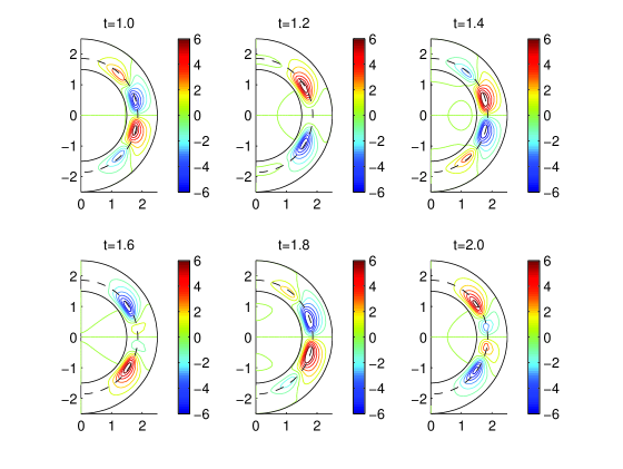
Figure 2: Rm=100. Contours of the azimuthal field $B_{\varphi}$ in a meridional plane at different time.

In the first simulation, we take $R_{\alpha}=30$, $R_{m}=100$, and plot in Figure 2 the contours of azimuthal field $B_{\varphi}$ in a meridional plane. In this simulation, we take $\delta t=\frac{1}{16000}$ with 40 equal spaced points for latitude and 40 equal spaced points for longitude, and 20 Legendre-Gaussian-Lobatto points in each layer. In Figure 3, we show the butterfly-shaped profile on the tachocline, where the function $f$ and internal differential rotation $u$ meet.

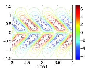
Figure 3: Butterfly diagram of azimuthal field at the interface at tachocline

In the second simulation, we keep $R_{\alpha}=30$ but take $R_{m}=1000$. and plot the contours of azimuthal field $B_{\varphi}$ in Figure 4. We observe similar quasi-periodic patterns as the previous example. The large $R_{m}$ leads to a significant increase of the magnitude.

In Figure 5, we plot magnetic energy $E_{m}=\int_{\Omega}|B|^{2}dx$ for $R_{\alpha}=30$ with different $R_{m}$. These results are consistent with those reported in [4].

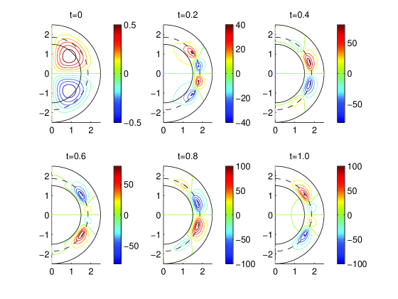
Figure 4: Rm=1000. Contours of the azimuthal field $B_{\varphi}$ in a meridional plane at different time.

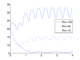
Figure 5: Energy for $R_{\alpha}=30,R_{m}=10,50,100$.

7 Concluding remarks

We developed in this paper an efficient numerical scheme for the 3D mean-field spherical dynamo equation. For the time discretization, we adopt a special semi-implicit discretization in such a way that at each time step one only needs to solve a linear system with piecewise constant coefficients. To deal with the divergence-free constraint, we use the divergence free vector spherical harmonic functions in space so that our numerical solution is automatically divergence-free. In addition, this allows us to reduce the linear system to be solved at each time step to a sequence of one-dimensional equations in the radial direction, which can then be solved by using a spectral-element method. Hence, the overall scheme is very efficient and accurate.

We showed that the solution of our fully discretized scheme remains bounded independent of the number of unknowns, and presented several numerical results to validate our scheme.

8 Acknowlegdegement

The research of T. Cheng is supported by NSF of China DOS 11871240 and DOS 11771170. The research of L. Ma is partially supported by NSF DMS-1913229. The research of J. Shen is partially supported by NSF DMS-1620262, DMS-1720442 and AFOSR FA9550-16-1-0102.

Appendix A Vector Spherical Harmonic basis

For VSH defined in (3.7)

$$\nabla\times\big{(}f{\boldsymbol{V}}_{l}^{m}\big{)}=\big{(}d_{l+2}^{+}f\big{)}{\boldsymbol{T}}_{l}^{m},$$

$$\nabla\times\big{(}f{\boldsymbol{W}}_{l}^{m}\big{)}=-\big{(}d_{l-1}^{-}f\big{)}{\boldsymbol{T}}_{l}^{m},$$

$$\nabla\times(f{\boldsymbol{T}}_{l}^{m})=\frac{l(l+1)f}{r}Y_{l}^{m}{\boldsymbol{e}}_{r}+\frac{1}{r}\frac{d(rf)}{dr}\nabla_{S}Y_{l}^{m}$$

$$(2l+1)\nabla\times\big{(}f{\boldsymbol{T}}_{l}^{m}\big{)}=(l+1)\big{(}d_{l+1}^{+}f\big{)}{\boldsymbol{W}}_{l}^{m}-l\big{(}d_{l}^{-}f\big{)}{\boldsymbol{V}}_{l}^{m},$$

$$\nabla\times\nabla\times(f(r){\boldsymbol{T}}_{l}^{m})=\left(\frac{l(l+1)f}{r^{2}}-\frac{2f^{\prime}}{r}-{f^{\prime\prime}}\right){\boldsymbol{T}}_{l}^{m}=\mathcal{L}(f){\boldsymbol{T}}_{l}^{m}.$$

Appendix B Representation of the Solenoidal Vector Field

We now seek the representation of the divergence free space, in other words, the Solenoidal vector field. We know that $\nabla\cdot{\bf curl}_{S}Y_{l}^{m}=0$, only need to see the other two sets.

Suppose we have a vector $\boldsymbol{u}$ represented by both sets of basis:

$$\begin{split}\boldsymbol{u}=&\sum_{l,m}a_{l}^{m}(r)Y_{l}^{m}{\boldsymbol{e}}_{r}+b_{l}^{m}(r)\nabla_{S}Y_{l}^{m}\\ =&\sum_{l,m}v_{l}^{m}(r){\boldsymbol{V}}_{l}^{m}+w_{l}^{m}(r){\boldsymbol{W}}_{l}^{m}\end{split}$$ (B.1)

Given identities

$$\nabla\cdot(f{\boldsymbol{T}}_{l}^{m})=0,\quad\nabla\cdot(f{\boldsymbol{V}}_{l}^{m})=(l+1)d_{l+2}^{+}fY_{l}^{m},$$ (B.2)

$$\nabla\cdot(f{\boldsymbol{W}}_{l}^{m})=ld_{l-1}^{-}fY_{l}^{m},$$ (B.3)

Divergence of the vector $\boldsymbol{u}$ given expansion under basis ${\boldsymbol{T}}_{l}^{m},{\boldsymbol{V}}_{l}^{m},{\boldsymbol{W}}_{l}^{m}$ is

$$\nabla\cdot\boldsymbol{u}=\sum_{l,m}[(l+1)d_{l+2}^{+}v_{l}^{m}+ld_{l-1}^{-}w_{l}^{m}]Y_{l}^{m}$$ (B.4)

We know that if $u$ is divergence free, it must obey the following relation,

$$(l+1)d_{l+2}^{+}v_{l}^{m}+ld_{l-1}^{-}w_{l}^{m}=0,\quad\forall l,m>0,$$ (B.5)

for $l=0$, we only have $\boldsymbol{V}_{0}^{0}$, therefore

$$d_{2}^{+}(a_{0}^{0}(r))=0.$$ (B.6)

Now we take divergence on $\boldsymbol{u}$.

$$\begin{split}\nabla\cdot\boldsymbol{u}=&\sum_{l,m}\frac{1}{r^{2}}\frac{\partial(r^{2}a_{l}^{m})}{\partial r}Y_{l}^{m}+\frac{1}{r\sin\theta}\frac{\partial}{\partial\theta}\left(\sin\theta b_{l}^{m}(r)\frac{\partial Y_{l}^{m}}{\partial\theta}\right)+\frac{1}{r\sin\theta}\frac{\partial}{\partial\varphi}\left(\frac{b_{l}^{m}(r)}{\sin\theta}\frac{\partial Y_{l}^{m}}{\partial\varphi}\right)\\ =&\sum_{l,m}\frac{1}{r^{2}}\frac{\partial(r^{2}a_{l}^{m})}{\partial r}Y_{l}^{m}+\frac{b_{l}^{m}(r)}{r\sin\theta}\frac{\partial}{\partial\theta}\left(\sin\theta\frac{\partial Y_{l}^{m}}{\partial\theta}\right)+\frac{b_{l}^{m}(r)}{r\sin^{2}\theta}\frac{\partial^{2}Y_{l}^{m}}{\partial\varphi^{2}}\\ =&\sum_{l,m}\frac{1}{r^{2}}\frac{\partial(r^{2}a_{l}^{m})}{\partial r}Y_{l}^{m}+\frac{b_{l}^{m}(r)}{r}\Delta_{S}Y_{l}^{m}=\sum_{l,m}\frac{1}{r^{2}}\frac{\partial(r^{2}a_{l}^{m})}{\partial r}Y_{l}^{m}-l(l+1)\frac{b_{l}^{m}(r)}{r}Y_{l}^{m}\end{split}$$ (B.7)

So we know for the solenoidal field, we need to have, $\forall l,m$,

$$r(a_{l}^{m})^{\prime}+2a_{l}^{m}-l(l+1)b_{l}^{m}=0$$ (B.8)

Consider the relations between $\{a_{l}^{m},b_{l}^{m}\}$ and $\{v_{l}^{m},w_{l}^{m}\}$ in (B.13)

$$(l+1)v_{l}^{m}+lw_{l}^{m}=a_{l}^{m},\quad w_{l}^{m}-v_{l}^{m}=b_{l}^{m}$$ (B.9)

$$v_{l}^{m}=\frac{a_{l}^{m}-lb_{l}^{m}}{2l+1},\quad w_{l}^{m}=\frac{a_{l}^{m}+(l+1)b_{l}^{m}}{2l+1}$$ (B.10)

So the coefficient for ${\boldsymbol{V}}_{l}^{m},{\boldsymbol{W}}_{l}^{m}$ should be:

$$v_{l}^{m}=-\frac{r}{(2l+1)(l+1)}d_{l-1}^{-}(a_{l}^{m}),\quad w_{l}^{m}=\frac{r}{l(2l+1)}d_{l+2}^{+}(a_{l}^{m})$$ (B.11)

or,

$$v_{l}^{m}=-\frac{1}{(2l+1)(l+1)}d_{l}^{-}(ra_{l}^{m}),\quad w_{l}^{m}=\frac{1}{l(2l+1)}d_{l+1}^{+}(ra_{l}^{m})$$ (B.12)

Let $A_{l}^{m}(r)=\frac{r}{l(l+1)}a_{l}^{m}(r)$, and notice the identities:

$$\begin{split}&{\bf curl}\big{(}f{\boldsymbol{V}}_{l}^{m}\big{)}=\big{(}d_{l+2}^{+}f\big{)}{\boldsymbol{T}}_{l}^{m},\quad{\bf curl}\big{(}f{\boldsymbol{W}}_{l}^{m}\big{)}=-\big{(}d_{l-1}^{-}f\big{)}{\boldsymbol{T}}_{l}^{m},\\ &(2l+1){\bf curl}\big{(}f{\boldsymbol{T}}_{l}^{m}\big{)}=(l+1)\big{(}d_{l+1}^{+}f\big{)}{\boldsymbol{W}}_{l}^{m}-l\big{(}d_{l}^{-}f\big{)}{\boldsymbol{V}}_{l}^{m}.\end{split}$$ (B.13)

Therefore we can rewrite $\boldsymbol{u}$ as:

$$\boldsymbol{u}={\bf curl}(\sum_{l,m}A_{l}^{m}(r){\boldsymbol{T}}_{l}^{m})$$ (B.14)

Now we know for any $\boldsymbol{u}$ in a solenoidal field, we can expand it as:

$$\boldsymbol{u}=\sum_{l,m}t_{l}^{m}(r){\boldsymbol{T}}_{l}^{m}+\nabla\times(A_{l}^{m}(r){\boldsymbol{T}}_{l}^{m})+a_{0}^{0}(r)Y_{0}^{0}{\boldsymbol{e}}_{r}$$ (B.15)

with $\displaystyle d_{2}^{+}a_{0}^{0}(r)=0$. For most practical cases, $a_{0}^{0}(r)$ is zero.

Appendix C Derivation of the Strong Form for Solenoidal Vector Field

We will give detailed derivation of the strong form in the solenoidal expansion in this section. The system is:

$$\alpha\boldsymbol{B}^{n}+\bar{\beta}\nabla\times\nabla\times B^{n}=\boldsymbol{f}_{1}+\nabla\times\boldsymbol{f}_{2},\quad{\rm in}\;\;\Omega,$$ (C.1)

with the boundary conditions

$$\begin{split}&\nabla\times\boldsymbol{b}^{n}\times\mathbf{n}=0,\quad\mbox{on}\quad{\partial\Omega},\\ &[\bar{\beta}\nabla\times\boldsymbol{b}^{n}\times\mathbf{n}]=\boldsymbol{g},\ [\boldsymbol{b}^{n}]=0\ \ \ \ \mbox{on}\;\;\Gamma_{1}\cup\Gamma_{2}.\end{split}$$ (C.2)

The expansions for functions involved are:

$$\boldsymbol{B}_{\boldsymbol{N}}(r,\theta,\varphi)=\sum_{i=1}^{3}\sum_{l=0}^{\infty}\sum_{|m|=0}^{l}u_{I_{i}}\Big{[}t_{l,m}^{i}(r){\boldsymbol{T}}_{l}^{m}(\theta,\varphi)+\nabla\times\Big{(}A_{l,m}^{i}(r){\boldsymbol{T}}_{l}^{m}(\theta,\varphi)\Big{)}\Big{]},$$ (C.3)

$$\boldsymbol{f}_{1}(r,\theta,\varphi)=\sum_{i=1}^{3}\sum_{l=0}^{\infty}\sum_{|m|=0}^{l}u_{I_{i}}\Big{[}f_{i,l,m}^{1,T}(r){\boldsymbol{T}}_{l}^{m}(\theta,\varphi)+f_{i,l,m}^{1,\nabla_{S}}(r)\nabla_{S}Y_{l}^{m}(\theta,\varphi)+f_{i,l,m}^{1,r}(r){\boldsymbol{e}}_{r}\Big{]},$$ (C.4)

$$\boldsymbol{f}_{2}(r,\theta,\varphi)=\sum_{i=1}^{3}\sum_{l=0}^{\infty}\sum_{|m|=0}^{l}u_{I_{i}}\Big{[}f_{i,l,m}^{2,T}(r){\boldsymbol{T}}_{l}^{m}(\theta,\varphi)+f_{i,l,m}^{2,\nabla_{S}}(r)\nabla_{S}Y_{l}^{m}(\theta,\varphi)+f_{i,l,m}^{2,r}(r){\boldsymbol{e}}_{r}\Big{]}.$$ (C.5)

$$\boldsymbol{g}_{i}(\theta,\varphi)=\sum_{l=0}^{\infty}\sum_{|m|=0}^{l}\Big{[}g_{i,l,m}^{T}(r){\boldsymbol{T}}_{l}^{m}(\theta,\varphi)+g_{i,l,m}^{\nabla_{S}}\nabla_{S}Y_{l,m}(\theta,\varphi)\Big{]},$$ (C.6)

After applying double curl on $\boldsymbol{B}_{N}$,

$$\nabla\times(\nabla\times\boldsymbol{B}_{N})=\sum_{i=1}^{3}\sum_{l=0}^{\infty}\sum_{|m|=0}^{l}u_{I_{i}}\Big{[}\mathcal{L}(t_{i,l,m}(r)){\boldsymbol{T}}_{l}^{m}+\frac{l(l+1)\mathcal{L}(A_{i,l,m}(r))}{r}Y_{l}^{m}{\boldsymbol{e}}_{r}$$ (C.7)

$$+\frac{1}{r}\frac{\partial\Big{(}r\mathcal{L}(A_{l}^{m}(r))\Big{)}}{\partial r}\nabla_{S}Y_{l}^{m}\Big{]}.$$ (C.8)

Direct calculation on $\nabla\times{\boldsymbol{f}}_{2}$ gives,

$$\nabla\times{\boldsymbol{f}}_{2}=\sum_{i=1}^{3}\sum_{l=0}^{\infty}\sum_{|m|=0}^{l}u_{I_{i}}\Big{[}\frac{l(l+1)f_{i,l,m}^{2,T}(r)}{r}Y_{l}^{m}(\theta,\varphi){\boldsymbol{e}}_{r}+\frac{1}{r}\frac{d(rf_{i,l,m}^{2,T}(r))}{dr}\nabla_{S}Y_{l}^{m}(\theta,\varphi)$$ (C.9)

$$-\frac{1}{r}\frac{d(rf_{i,l,m}^{2,\nabla_{S}}(r))}{dr}{\boldsymbol{T}}_{l}^{m}(\theta,\varphi)+\frac{f_{i,l,m}^{2,r}(r)}{r}{\boldsymbol{T}}_{l}^{m}(\theta,\varphi)\Big{]}.$$ (C.10)

Due to the othorganality of ${\boldsymbol{T}}_{l}^{m},Y_{l}^{m}\boldsymbol{e}_{r}$ and $\nabla_{S}Y_{l}^{m}$, it is easy to derive that for ${\boldsymbol{T}}_{l}^{m}$ direction,

$$\alpha t_{i,l,m}(r)+\bar{\beta}_{i}\mathcal{L}(t_{i,l,m}(r))=f_{i,l,m}^{1,T}(r)+\frac{f_{i,l,m}^{2,r}(r)}{r}-\frac{1}{r}\frac{d(rf_{i,l,m}^{2,\nabla_{S}}(r))}{dr},\;\;{\rm in}\;\;I_{i},$$ (C.11)

for $\nabla_{S}Y_{l}^{m}$ direction,

$$\alpha\frac{1}{r}\frac{d(rA_{i,l,m}(r))}{dr}+\bar{\beta}\frac{1}{r}\frac{d\Big{(}r\mathcal{L}A_{i,l,m}(r)\Big{)}}{dr}=f_{i,l,m}^{1,\nabla_{S}}(r)+\frac{1}{r}\frac{d(rf_{i,l,m}^{2,T}(r))}{dr},$$ (C.12)

for ${\boldsymbol{e}}_{r}$ direction,

$$\alpha A_{i,l,m}(r)+\bar{\beta}_{i}\mathcal{L}(A_{i,l,m}(r))=\frac{r}{l(l+1)}f_{i,l,m}^{1,r}(r)+f_{i,l,m}^{2,T}(r).\;\;{\rm in}\;\;I_{i}.$$ (C.13)

Notice the fact that $\boldsymbol{f}_{1}$ is also in the solenoidal vector field, which means

$$\frac{1}{r^{2}}\frac{d(r^{2}f_{l,m}^{1,r})}{dr}=\frac{l(l+1)}{r}f_{l,m}^{1,\nabla_{S}},$$ (C.14)

(C.12) can be rewritten as:

$$\alpha\frac{1}{r}\frac{d(rA_{i,l,m}(r))}{dr}+\bar{\beta}\frac{1}{r}\frac{d\Big{(}r\mathcal{L}A_{i,l,m}(r)\Big{)}}{dr}=\frac{1}{r}\frac{d}{dr}(\frac{r^{2}f_{i,l,m}^{1,r}(r)}{l+1})+\frac{1}{r}\frac{d(rf_{i,l,m}^{2,T}(r))}{dr},$$ (C.15)

We want to make a remark that (C.13) and (C.15) differ in the order of the PDE in the sense that solution of $A_{i,l,m}(r)$ can differ up to a constant. We have already pointed out that in the solenoidal representation, the $A(r)$ is not unique, but we can manually set the constant to any value for convenience.

We focus now on the boundary conditions. First we consider

$$[\boldsymbol{b}_{N}]=0,$$

this requires the continuity at intersections, which leads to the following conditions. For ${\boldsymbol{T}}_{l}^{m}$ direction:

$$t_{1,l,m}(a)=t_{2,l,m}(a),\;\;t_{2,l,m}(b)=t_{3,l,m}(b),$$ (C.16)

for $\nabla_{S}Y_{l}^{m}$ direction:

$$\frac{d}{dr}(rA_{1,l,m}(r))\Big{|}_{r=a}=\frac{d}{dr}(rA_{2,l,m}(r))\Big{|}_{r=a},\;\;\frac{d}{dr}(rA_{2,l,m}(r))\Big{|}_{r=b}=\frac{d}{dr}(rA_{3,l,m}(r))\Big{|}_{r=b}$$ (C.17)

for $Y_{l}^{m}\boldsymbol{e}_{r}$ direction:

$$A_{1,l,m}(a)=A_{2,l,m}(a),\;\;A_{2,l,m}(b)=A_{3,l,m}(b).$$ (C.18)

Next, we consider

$$[\nabla\times\boldsymbol{b}_{N}\times\boldsymbol{n}]=\boldsymbol{g},$$

which will leads to for ${\boldsymbol{T}}_{l}^{m}$ direction:

$$\bar{\beta}_{1}d_{1}^{+}t^{1}_{l,m}(a)-\bar{\beta}_{2}d_{1}^{+}t^{2}_{l,m}(a)=g^{T}_{1,l,m},$$ (C.19)

$$\bar{\beta}_{3}d_{1}^{+}t^{3}_{l,m}(b)-\bar{\beta}_{2}d_{1}^{+}t^{2}_{l,m}(b)=g^{T}_{2,l,m},$$ (C.20)

for $\nabla_{S}Y_{l}^{m}$ direction:

$$\bar{\beta}_{2}\mathcal{L}(A_{2,l,m}(a))-\bar{\beta}_{1}\mathcal{L}(A_{1,l,m}(a))=g^{\nabla_{S}}_{1,l,m},$$ (C.21)

$$\bar{\beta}_{2}\mathcal{L}(A_{2,l,m}(b))-\bar{\beta}_{3}\mathcal{L}(A_{3,l,m}(b))=g^{\nabla_{S}}_{2,l,m},$$ (C.22)

and no condition can be given in the $\boldsymbol{e}_{r}$ direction.
On $\Gamma_{3}$, the boundary condition is:

$$\nabla\times\boldsymbol{b}_{N}\times\boldsymbol{n}=0,$$

this leads to

$$d_{1}^{+}t^{3}_{l,m}(c)=0,\quad\mathcal{L}_{l}(A^{3}_{l,m})(c)=0.$$ (C.23)

It is quite clear the for $\nabla_{S}Y_{l}^{m}$ and $Y_{l}^{m}\boldsymbol{e}_{r}$ directions, the differential equations are essentially the same but boundary conditions differ a lot. This is because the $\boldsymbol{e}_{r}$ direction is a consequence in the solenoidal vector field. We will take the $\nabla_{S}Y_{l}^{m}$ as the first choice, and still taking account the boundary conditions for $\boldsymbol{e}_{r}$ direction.

Now we can summarize the strong form for $t_{i,l,m}(r)$ and $A_{i,l,m}(r)$.

$$\alpha t_{i,l,m}(r)+\bar{\beta}_{i}\mathcal{L}(t_{i,l,m}(r))=f_{i,l,m}^{1,T}(r)+\frac{f_{i,l,m}^{2,r}(r)}{r}-\frac{1}{r}\frac{d(rf_{i,l,m}^{2,\nabla_{S}}(r))}{dr},\;\;{\rm in}\;\;I_{i},$$ (C.24)

$$t_{1,l,m}(a)=t_{2,l,m}(a),\;\;t_{2,l,m}(b)=t_{3,l,m}(b),$$ (C.25)

$$\bar{\beta}_{1}d_{1}^{+}t^{1}_{l,m}(a)-\bar{\beta}_{2}d_{1}^{+}t^{2}_{l,m}(a)=g^{T}_{1,l,m},$$ (C.26)

$$\bar{\beta}_{3}d_{1}^{+}t^{3}_{l,m}(b)-\bar{\beta}_{2}d_{1}^{+}t^{2}_{l,m}(b)=g^{T}_{2,l,m},$$ (C.27)

$$d_{1}^{+}t^{3}_{l,m}(c)=0.$$ (C.28)

$$\alpha(rA_{i,l,m}(r))^{\prime}+\bar{\beta}\Big{(}r\mathcal{L}A_{i,l,m}(r)\Big{)}^{\prime}=rf_{i,l,m}^{1,\nabla_{S}}(r)+(rf_{i,l,m}^{2,T}(r))^{\prime},$$ (C.29)

$$A_{1,l,m}(a)=A_{2,l,m}(a),\;\;A_{2,l,m}(b)=A_{3,l,m}(b),$$ (C.30)

$$A_{1,l,m}^{\prime}(a)=A_{2,l,m}^{\prime}(a),\;\;A_{2,l,m}^{\prime}(b)=A_{3,l,m}^{\prime}(b),$$ (C.31)

$$\bar{\beta}_{2}\mathcal{L}(A_{2,l,m}(a))-\bar{\beta}_{1}\mathcal{L}(A_{1,l,m}(a))=g^{\nabla_{S}}_{1,l,m},$$ (C.32)

$$\bar{\beta}_{2}\mathcal{L}(A_{2,l,m}(b))-\bar{\beta}_{3}\mathcal{L}(A_{3,l,m}(b))=g^{\nabla_{S}}_{2,l,m},$$ (C.33)

$$\mathcal{L}_{l}(A^{3}_{l,m})(c)=0.$$ (C.34)

References

- [1] Garth A Baker, Wadi N Jureidini, and Ohannes A Karakashian. Piecewise solenoidal vector fields and the stokes problem. SIAM journal on numerical analysis, 27(6):1466–1485, 1990.
- [2] R. A. Bayliss, C. B. Forest, M. D. Nornberg, E. J. Spence, and P. W. Terry. Numerical simulations of current generation and dynamo excitation in a mechanically forced turbulent flow. Phys. Rev. E (3), 75(2):026303, 13, 2007.
- [3] Edward Crisp Bullard and H Gellman. Homogeneous dynamos and terrestrial magnetism. Phil. Trans. R. Soc. Lond. A, 247(928):213–278, 1954.
- [4] K. Chan, K. Zhang, and J. Zou. Spherical interface dynamos: Mathematical theory, finite element approximation, and application. SIAM Journal on Numerical Analysis, 44(5):1877–1902, 2006.
- [5] Kit H Chan, Keke Zhang, Jun Zou, and Gerald Schubert. A nonlinear vacillating dynamo induced by an electrically heterogeneous mantle. Geophysical Research Letters, 28(23):4411–4414, 2001.
- [6] Vivette Girault and Pierre-Arnaud Raviart. Finite element methods for Navier-Stokes equations, volume 5 of Springer Series in Computational Mathematics. Springer-Verlag, Berlin, 1986. Theory and algorithms.
- [7] C. Guervilly and P. Cardin. Numerical simulations of dynamos generated in spherical Couette flows. Geophys. Astrophys. Fluid Dyn., 104(2-3):221–248, 2010.
- [8] E.L. Hill. The theory of vector spherical harmonics. Amer. J. Phys., 22:211–214, 1954.
- [9] R. Hollerbach. On the theory of the geodynamo. Physics of the Earth and Planetary interiors, 98(3):163–185, 1996.
- [10] Rainer Hollerbach. A spectral solution of the magneto-convection equations in spherical geometry. International journal for numerical methods in fluids, 32(7):773–797, 2000.
- [11] Chris A. Jones. Planetary magnetic fields and fluid dynamos. In Annual review of fluid mechanics. Volume 43, 2011, volume 43 of Annu. Rev. Fluid Mech., pages 583–614. Annual Reviews, Palo Alto, CA, 2011.
- [12] Ohannes A Karakashian and Wadi N Jureidini. A nonconforming finite element method for the stationary Navier–Stokes equations. SIAM journal on numerical analysis, 35(1):93–120, 1998.
- [13] W. Kuang and J. Bloxham. Numerical modeling of magnetohydrodynamic convection in a rapidly rotating spherical shell: weak and strong field dynamo action. Journal of Computational Physics, 153(1):51–81, 1999.
- [14] David Moss. Numerical simulation of the Gailitis dynamo. Geophys. Astrophys. Fluid Dyn., 100(1):49–58, 2006.
- [15] C-D Munz, Pascal Omnes, Rudolf Schneider, Eric Sonnendrücker, and Ursula Voss. Divergence correction techniques for Maxwell solvers based on a hyperbolic model. Journal of Computational Physics, 161(2):484–511, 2000.
- [16] J.C. Nédélec. Acoustic and Electromagnetic Equations, volume 144 of Applied Mathematical Sciences. Springer-Verlag, New York, 2001. Integral representations for harmonic problems.
- [17] Mohammad M. Rahman and David R. Fearn. A spectral solution of nonlinear mean field dynamo equations: with inertia. Comput. Math. Appl., 58(3):422–435, 2009.
- [18] Mohammad M. Rahman and David R. Fearn. A spectral solution of nonlinear mean field dynamo equations: without inertia. Commun. Nonlinear Sci. Numer. Simul., 15(9):2552–2564, 2010.
- [19] Paul H. Roberts, Gary A. Glatzmaier, and Thomas L. Clune. Numerical simulation of a spherical dynamo excited by a flow of von Kármán type. Geophys. Astrophys. Fluid Dyn., 104(2-3):207–220, 2010.
- [20] Michel Sermange and Roger Temam. Some mathematical questions related to the MHD equations. Comm. Pure Appl. Math., 36(5):635–664, 1983.
- [21] Ozan Tuğluk and Hakan I Tarman. Direct numerical simulation of pipe flow using a solenoidal spectral method. Acta Mechanica, 223(5):923–935, 2012.
- [22] Kane Yee. Numerical solution of initial boundary value problems involving Maxwell’s equations in isotropic media. IEEE Transactions on antennas and propagation, 14(3):302–307, 1966.
- [23] K Zhang, KH Chan, J Zou, X Liao, and G Schubert. A three-dimensional spherical nonlinear interface dynamo. The Astrophysical Journal, 596(1):663, 2003.
- [24] K-K Zhang and FH Busse. Convection driven magnetohydrodynamic dynamos in rotating spherical shells. Geophysical & Astrophysical Fluid Dynamics, 49(1-4):97–116, 1989.