Cloud-Assisted Contracted Simulation of Quantum Chains

Abstract

The work discusses validation of properties of quantum circuits with many qubits using non-universal set of quantum gates ensuring possibility of effective simulation on classical computer. An understanding analogy between different models of quantum chains is suggested for clarification. An example with IBM Q Experience cloud platform and Qiskit framework is discussed finally.

I Introduction

A question about compliance with the model of scalable gate-based quantum computations desirable for generally known algorithms from BQP (bounded-error quantum polynomial time) complexity class BQP encounters certain difficulties already for not very big amount of qubits, because of problems with direct verification of results even using modern supercomputers.

The discussions about “quantum supremacy” supr milestone rather emphasize such a controversy, because it requires comparison between some quantum devices and state-of-art classical simulators simsupr . Different methods to address such a problem could be suggested. Well-known example is random sampling using appropriate (universal) set of quantum gates together with statistical analysis of final states of qubits blue . An alternative approach is looking for “quantum agreement” with a specific quantum circuits with restricted (non-universal) sets of gates generating entanglement of hundreds or even thousands qubits, but effectively modelled by classical computers.

One possible example is specific version of logarithmic space bounded quantum computations implemented by so-called matchgates val ; log . In such a case some non-universal quantum circuit with $d$ qubits can be “contracted” into universal one with only $l=\lceil\log_{2}(d)\rceil$ qubits. Simplified version of such approach using illustrative example with quantum chains is discussed below.

II Quantum Chains

A correspondence between two models is used in presented work. The first one is a chain with $d$ qubits (Figure 1). The space of states for such a model has dimension $2^{d}$.

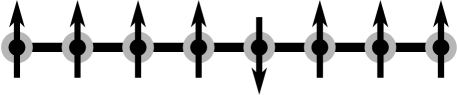
Figure 1: Qubit (spin) chain.

The second model is a quantum scalar chain with $d$ nodes (Figure 2) with only $d$ states that can be considered as a single “qudit,” that is, in turn, could be ‘contracted’ (‘compressed’) into $l=\lceil\log_{2}(d)\rceil$ qubits.

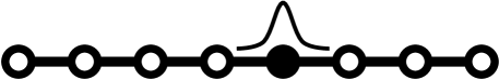
Figure 2: Quantum scalar chain.

Let us consider quantum system with Hamiltonian

$$\hat{\mathcal{H}}=\sum_{j=0}^{d-2}\frac{\lambda_{j}}{2}(\hat{\sigma}^{x}_{j}\hat{\sigma}^{x}_{j+1}+\hat{\sigma}^{y}_{j}\hat{\sigma}^{y}_{j+1})+\sum_{j=0}^{d-2}\frac{\chi_{j}}{2}(\hat{\sigma}^{y}_{j}\hat{\sigma}^{x\vphantom{y}}_{j+1}-\hat{\sigma}^{x\vphantom{y}}_{j}\hat{\sigma}^{y}_{j+1})+\sum_{k=0}^{d-1}\mu_{k}\hat{\sigma}^{z}_{k}.$$ (1)

It should be mentioned, that the Hamiltonian Eq. (1) does not include forth order terms required for generation of universal set of quantum gates (cf analogue expression in Ref. blue ).

It may be checked directly, that Eq. (1) commutes with ‘number operator’

$$\hat{\mathcal{N}}=\sum_{k=0}^{d-1}\frac{\hat{\openone}-\hat{\sigma}^{z}_{k}}{2}$$ (2)

Thus, number ${\mathcal{N}}$ of units in computational basis is conserved by quantum gates $\hat{\mathcal{G}}=\exp(-i\hat{\mathcal{H}}\Delta t)$ generated by Hamiltonians Eq. (1). Here $\Delta t$ is time interval of application for given $\hat{\mathcal{H}}$ and the natural system of units with $\hbar=1$ is used in all equations.

The states with $\mathcal{N}=1$ simply correspond to $d$ basic states of quantum scalar chain with respect to map

$$|k\rangle\mapsto\bigl{|}\underbrace{0\ldots 0}_{k}1\underbrace{0\ldots 0}_{d-k-1}\bigr{\rangle},\quad k=0,\ldots,d-1.$$ (3)

For qubit chain conservation of $\mathcal{N}$ conforms to restricted case of matchgate circuits TD2 ; AV18 and it is represented below by two-qubit gates such as $\hat{\mathcal{M}}$ in Eq. (18) or Eq. (22).

The term ‘matchgate’ was introduced in val for a quantum two-gate of special form Eq. (17) recollected below. The considered model is also naturally represented using relation between $Spin(2d)$ groups and orthogonal transformations in dimension $2d$ AV18 . In general, conservation of $\mathcal{N}$ is not mandatory, but it is discussed elsewhere TD2 ; AV18 .

Similar approach with compressed quantum computation was tested on IBM Q Experience cloud platform compr . In such a case 5-qubits quantum chip was used for simulation of quantum Ising chain with $2^{5}=32$ spins and for testing was used correspondence between $2$ and $2^{2}=4$ qubits with rather pessimistic results for current error level.

The term contracted quantum simulation is chosen here because, from the one hand, exponentially smaller (‘contracted’) model is used for testing. On the other hand, it provides informal reference to idea of reliable design-by-contract contr with natural tests (‘contracts’) for appropriate functionality. It may be useful for testing both quantum chips and classical simulators of quantum computer.

The modelling was performed by author with IBM Q Experience Qiskit qiskit framework providing common environment for work with a few real quantum chips and simulation both on hight performance computer (HPC) in the cloud and personal computer (PC). Discussed model with chains is included in the community tutorials for Qiskit chain-tut and it is revisited in the next section. More recent updates and extensions may be found in separate repository for quantum chain models quchain .

III Quantum Walk Simulation

III.1 Discrete-time quantum walks

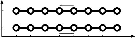
Figure 3: Space of states for coined quantum walk

Model with continuous evolution described by Hamiltonian (1) is not adapted for implementation with quantum circuits. However, model of coined quantum walks after appropriate reformulation for qubit chain also may be described using similar approach AV18 and it can be used here with the similar purposes.

Let us start with usual model of discrete-time quantum walks for scalar quantum chains with further reformulation to quantum circuit model using correspondence Eq. (3). Coined quantum walk Kem03 is naturally defined for composite quantum system with a chain $|k\rangle$, $k=0,\ldots,n-1$ and coin $|c\rangle$, $c=0,1$. The basic states of such a system can be expressed as $|c\rangle|k\rangle$ and the dimension of space of states is $d=2n$. The coin and chain states are depicted on Figure 3 along vertical and horizontal axes respectively.

Let us consider operators of right and left shift on the chain $\hat{\mathcal{R}}$ and $\hat{\mathcal{L}}$ together with an operator acting on composite system

$$\hat{\mathcal{B}}=|0\rangle\langle 0|\otimes\hat{\mathcal{R}}+|1\rangle\langle 1|\otimes\hat{\mathcal{L}}.$$ (4)

The operator $\hat{\mathcal{B}}$ (‘quantum bot’ qubot ) could be considered as an example of conditional quantum dynamics cond95 with chain as a target and coin as control. For simplest case without superposition of coin states it applies operators $\hat{\mathcal{R}}$ or $\hat{\mathcal{L}}$ to chain for states of coin $|0\rangle$ or $|1\rangle$ respectively. For finite chains the periodic boundary conditions may be considered first for simplicity, see Figure 4.

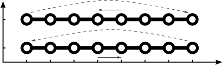
Figure 4: Periodic boundary conditions

Coined quantum walk has more complex dynamics due to additional ‘coin toss’ operator $\hat{\mathcal{C}}$ acting on the control space. The standard choice for $\hat{\mathcal{C}}$ is Hadamard coin

$$\hat{\mathcal{C}}_{\rm H}=\frac{\sqrt{2}}{2}\left(\begin{array}[]{rr}1&1\\ 1&-1\end{array}\right)$$ (5)

or balanced coin

$$\hat{\mathcal{C}}_{\rm b}=\frac{\sqrt{2}}{2}\begin{pmatrix}1&i\\ i&1\end{pmatrix}.$$ (6)

Taking into account such operator the single step of quantum walk can be expressed as composition of $\hat{\mathcal{B}}$ and coin toss operator $\hat{\mathcal{C}}$

$$\hat{\mathcal{W}}=(\hat{\mathcal{C}}\otimes\hat{\openone})\,\hat{\mathcal{B}},$$ (7)

where $\hat{\openone}$ is the identity operator on a chain and $\hat{\mathcal{C}}$ is a coin toss operator such as Eq. (5) or Eq. (6).

The cyclic (periodic) boundary conditions may be not very convenient for implementation with neighbouring nodes mapped into qubit chain with nearest-neighbour quantum gates discussed below. The operator $\hat{\mathcal{B}}$ can be modified for reflecting boundary conditions corresponding to change of direction due to ‘flip’ on the ends of chains, see Figure 5.

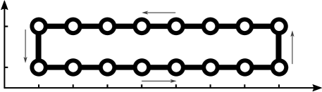
Figure 5: Reflecting boundary conditions

For restriction of each operator to neighbouring nodes such a model can be represented as so-called staggered quantum walk stag on a chain with $d=2n$ nodes using correspondence

$$|c\rangle|k\rangle\longleftrightarrow|2k+c\rangle;\qquad k=0,\ldots,d-1;\quad c=0,1.$$ (8)

Let us consider such a chain with partitions depicted on a Figure 6 and a transformation produced by alternating swaps with pairs of nodes from first and second partition outlined by solid and dashed ellipses respectively.

Figure 6: Partition for staggered quantum walk

Let us express swap of two nodes using Pauli matrix

$$\hat{X}=\hat{\sigma}_{x}=\begin{pmatrix}0&1\\ 1&0\end{pmatrix}.$$ (9)

In such a case swap of all pairs in the first partition corresponds to operator

$$\hat{\mathcal{B}}_{1}=\hat{X}_{(0,1)}\hat{X}_{(2,3)}\cdots\hat{X}_{(d-2,d-1)},$$ (10)

there each operator in the expression swaps two nodes with indexes shown in brackets. An analogue expression for the second partition is

$$\hat{\mathcal{B}}_{2}=\hat{X}_{(1,2)}\hat{X}_{(3,4)}\cdots\hat{X}_{(d-3,d-2)}.$$ (11)

It may be checked directly, that with respect to map Eq. (8) the composition of $\hat{\mathcal{B}}_{1}$ and $\hat{\mathcal{B}}_{2}$ implements operator $\hat{\mathcal{B}}$ for reflecting boundary condition.

The coin toss operator for a model of staggered quantum walk can be implemented by application of the $\hat{\mathcal{C}}$ to each pair of nodes from the first partition and may be expressed as

$$\hat{\mathcal{C}}_{1}=\hat{\mathcal{C}}_{(0,1)}\hat{\mathcal{C}}_{(2,3)}\cdots\hat{\mathcal{C}}_{(d-2,d-1)}.$$ (12)

In such a way the staggered walk is represented by composition of three operators $\hat{\mathcal{C}}_{1}$, $\hat{\mathcal{B}}_{1}$ and $\hat{\mathcal{B}}_{2}$ acting only on neighbouring nodes. The operators $\hat{\mathcal{C}}$ and $\hat{\mathcal{B}}_{1}$ act on the same pairs of nodes and expression may be simplified by modification of coin toss operator

$$\hat{\mathcal{C}}^{\prime}=\hat{\mathcal{C}}\hat{X}$$ (13)

with straightforward action on the first partition

$$\hat{\mathcal{C}}^{\prime}_{1}=\hat{\mathcal{C}}^{\prime}_{(0,1)}\hat{\mathcal{C}}^{\prime}_{(2,3)}\cdots\hat{\mathcal{C}}^{\prime}_{(d-2,d-1)}.$$ (12^′)

For example with Hadamard coin modified operator is

$$\hat{\mathcal{C}}^{\prime}_{\rm H}=\hat{\mathcal{C}}_{H}\hat{X}=\frac{\sqrt{2}}{2}\left(\begin{array}[]{rr}1&1\\ -1&1\end{array}\right).$$ (14)

Thus, staggered walk is represented by composition of operators Eq. (12^′) and Eq. (11)

$$\hat{\mathcal{W}}_{s}=\hat{\mathcal{C}}^{\prime}_{1}\,\hat{\mathcal{B}}_{2}.$$ (15)

III.2 Modelling of qubit chain

The staggered walk on the chain can be simply implemented by Python program without any special libraries for simulation of quantum circuits, but analogue model with qubit chain is using Qiskit. Let us consider map Eq. (3) introduced earlier to work with qubit chain. Operators acting on neighbouring nodes in such a case correspond to special case of matchgates.

Let us consider two unitary operators $\hat{u}$ and $\hat{v}$ represented by $2\times 2$ matrices with equal determinants

$$\hat{v}=\begin{pmatrix}v_{00}&v_{01}\\ v_{10}&v_{11}\end{pmatrix},\quad\hat{u}=\begin{pmatrix}u_{00}&u_{01}\\ u_{10}&u_{11}\end{pmatrix},\quad\det\hat{v}=\det{\hat{u}}$$ (16)

By definition the matchgate is two-gate on near neighbour qubits expressed as $4\times 4$ matrix produced from elements Eq. (16) of $\hat{v}$ and $\hat{u}$

$$\hat{\mathcal{M}}_{v,u}=\begin{pmatrix}v_{00}&0&0&v_{01}\\ 0&u_{00}&u_{01}&0\\ 0&u_{10}&u_{11}&0\\ v_{10}&0&0&v_{11}\end{pmatrix}.$$ (17)

Let us consider special case with $\hat{v}=\hat{\openone}$ and $\det\hat{u}=1$

$$\hat{\mathcal{M}}_{u}=\begin{pmatrix}1&0&0&0\\ 0&u_{00}&u_{01}&0\\ 0&u_{10}&u_{11}&0\\ 0&0&0&1\end{pmatrix}.$$ (18)

Such matchgates are two-gates with non-trivial action only for superpositions with states $|01\rangle$ and $|10\rangle$ of neighbouring qubits. It may be generated by Hamiltonians Eq. (1) with terms corresponding to considered pair of qubits. With respect to map Eq. (3) it is equivalent with operator $\hat{u}$ acting on two neighbouring nodes.

For Hadamard coin ‘swapped’ operator $\hat{\mathcal{C}}^{\prime}_{\rm H}$ Eq. (14) has unit determinant and can be directly used for construction of matchgate

$$\mathcal{\hat{M}_{C}^{\prime}}=\begin{pmatrix}1&0&0&0\\ 0&1/\sqrt{2}&1/\sqrt{2}&0\\ 0&-1/\sqrt{2}&1/\sqrt{2}&0\\ 0&0&0&1\end{pmatrix}.$$ (19)

Such a gates should be applied to all pair of qubits in the first partition similarly with Eq. (12^′)

There is some subtlety, because swap operator does not have unit determinant $\det(\hat{X})=-1$ and operator $i\hat{X}$ with unit determinant was used instead. Thus, two qubit-gates for a single swap is modified as

$$\hat{\mathcal{M}}_{iX}=\begin{pmatrix}1&0&0&0\\ 0&0&i&0\\ 0&i&0&0\\ 0&0&0&1\end{pmatrix}.$$ (20)

Application of such a gate for all pairs of qubits in the second partition is analogue of Eq. (11).

Single-qubit gates in Qiskit and quantum assembly language OpenQASM OpenQASM are parametrized using three angles

$$\hat{\mathcal{U}}(\theta,\phi,\lambda)=\begin{pmatrix}e^{-i(\phi+\lambda)/2}\cos(\theta/2)&-e^{-i(\phi-\lambda)/2}\sin(\theta/2)\\ e^{i(\phi-\lambda)/2}\sin(\theta/2)&e^{i(\phi+\lambda)/2}\cos(\theta/2)\end{pmatrix}.$$ (21)

With similar parametrization $\hat{\mathcal{M}}_{u}$ Eq. (18) can be rewritten

$$\hat{\mathcal{M}}(\theta,\phi,\lambda)=\begin{pmatrix}1&0&0&0\\ 0&e^{-i(\phi+\lambda)/2}\cos(\theta/2)&-e^{-i(\phi-\lambda)/2}\sin(\theta/2)&0\\ 0&e^{i(\phi-\lambda)/2}\sin(\theta/2)&e^{i(\phi+\lambda)/2}\cos(\theta/2)&0\\ 0&0&0&1\end{pmatrix}.$$ (22)

Now gates Eq. (19) and Eq. (20) can be rewritten

$$\mathcal{\hat{M}_{C}^{\prime}}=\hat{\mathcal{M}}(-\pi/2,0,0),\quad\hat{\mathcal{M}}_{iX}=\hat{\mathcal{M}}(\pi,\pi,0)$$ (23)

With OpenQASM notation the two-qubit gate Eq. (22) can be expressed as a sequence of single-qubit gates Eq. (21) (denoted as U) and controlled NOT gates (denoted as cx).

M(theta, phi, lambda) a,b {
  cx a,b;
  U(0,0,(lambda-phi)/2) a;
  cx b,a;
  U(-theta/2,0,-(phi+lambda)/2) a;
  cx b,a;
  U(theta/2,phi,0) a;
  cx a,b;
}

Here variables in brackets are parameters and a, b are indexes of qubits. Thus, such a function can be applied using parameters from Eq. (23) to necessary pairs of qubits. Qiskit uses analogue approach with definition of function in Python language.

References

- (1) E. Bernstein and U. Vazirani, SIAM J. Comput. 26, 1411 (1997).
- (2) J. Preskill, e-print arXiv:1203.5813 [quant-ph] (2012).
- (3) B. Villalonga, et al., e-print arXiv:1905.0444 [quant-ph] (2019).
- (4) C. Neil, et al., Science 365, 195 (2018).
- (5) L. G. Valiant, Proc. 33rd Annual ACM STOC, 114–123 (2001).
- (6) R. Jozsa, B. Kraus, A. Miyake, and J. Watrous, Proc. R. Soc. A 466, 809 (2010).
- (7) B. M. Terhal and D. P. DiVincenzo, Phys. Rev. A 65, 032325 (2002).
- (8) A. Yu. Vlasov, Quant. Inf. Proc. 17, 269 (2018).
- (9) M. Hebenstreit, D. Alsina, J. I. Latorre, and B. Kraus, Phys. Rev. A 95, 052339 (2017).
- (10) B. Meyer, Computer (IEEE) 25(10), 40 (1992).
- (11) H. Abraham et al., Qiskit: An Open-source Framework for Quantum Computing (2019), DOI:10.5281/zenodo.2562110.
-
(12)
A. Yu. Vlasov, “State Distribution in Quantum Chains,” in Qiskit community tutorials,
https://github.com/Qiskit/qiskit-community-tutorials - (13) https://qubeat.github.io/quchain
- (14) J. Kempe, Contemp. Phys. 44, 307 (2003).
- (15) A. Yu. Vlasov, “Quantum bots on lattices,” (2000), talk at Think-tank on Computer Science Aspects, Torino, Italy.
- (16) A. Barenco, D. Deutsch, A. K. Ekert, and R. Jozsa, Phys. Rev. Lett. 74, 4083 (1995).
- (17) R. Portugal, Quant. Inform. Proc. 15(4), 1387 (2016).
- (18) A. W. Cross, L. S. Bishop, J. A. Smolin, and J. M. Gambetta, e-print arXiv:1707.03429v2 [quant-ph] (2017).