D-Modules and Holonomic Functions

D-Modules and Holonomic Functions Anna-Laura Sattelberger and Bernd Sturmfels MPI-MiS Leipzig and MPI-MiS Leipzig/UC Berkeley anna-laura.sattelberger@mis.mpg.de and bernd@mis.mpg.de Anna-Laura Sattelberger and Bernd Sturmfels In algebraic geometry, one studies the solutions to polynomial equations, or, equivalently, to linear partial differential equations with constant coefficients. These lecture notes address the more general case when the coefficients of the partial differential equations are polynomials. The letter $D$ stands for the Weyl algebra, and a $D$-module is a left module over $D$. We focus on left ideals, or $D$-ideals. We represent holonomic functions in several variables by the linear differential equations they satisfy. This encoding by a $D$-ideal is useful for many problems, e.g., in geometry, physics and statistics. We explain how to work with holonomic functions. Applications include volume computations and likelihood inference.

Introduction

This article represents the notes for the three lectures delivered by the second author at the Math+ Fall School in Algebraic Geometry, held at FU Berlin from September 30 to October 4, 2019. The aim was to give an introduction to $D$-modules and their use for concrete problems in applied algebraic geometry. This centers around the concept of a holonomic function in several variables. Such a function is among the solutions to a system of linear partial differential equations whose solution space is finite-dimensional. Our algebraic representation as a $D$-ideal allows us to perform many operations with such objects.

The three lectures form the three sections of this article. In the first lecture, we introduce the basic tools. The focus is on computations that are built on Gröbner bases in the Weyl algebra. We review the Fundamental Theorem of Algebraic Analysis, we introduce holonomic $D$-ideals, and we discuss their holonomic rank. Our presentation of these topics is based on the book [SST00].

In the second lecture, we study the problem of measuring areas and volumes of semi-algebraic sets. These quantities are represented as integrals, and our task is to evaluate such an integral as accurately as is possible. To do so, we follow the approach of Lairez, Mezzarobba, and Safey El Din [LMSED19]. We introduce a parameter into the integrand, and we regard our integral as a function in that parameter. Such a volume function is holonomic, and we derive a $D$-ideal that annihilates it. Using manipulations with that $D$-ideal, we arrive at a scheme that allows for highly accurate numerical evaluation of the relevant integrals.

The third lecture is about connections to statistics. Many special functions arising in statistical inference are holonomic. We start out with likelihood functions for discrete models and their Bernstein–Sato polynomials, and we then discuss the holonomic gradient method and holonomic gradient descent. These were developed by a group of Japanese scholars [HNTT13, STT⁺10] for representing, evaluating and optimizing functions arising in statistics. We give an introduction to this theory, aiming to highlight opportunities for further research. Our readers can hone their holonomic skills with a list of $19$ problems at the end of these lecture notes. We also provide hints and solutions to solve the problems.

0.1 Tools

Our presentation follows closely the one in [SST00, Tak13], albeit we use a slightly different notation. For any integer $n\geq 1$, we introduce the $n$th Weyl algebra with complex coefficients:

$$D\,\,=\,\,\mathbb{C}\left[x_{1},\ldots,x_{n}\right]\langle\partial_{1},\ldots,\partial_{n}\rangle.$$

We sometimes write $D_{n}$ instead of $D$ if we want to highlight the dimension $n$ of the ambient space. For the sake of brevity, we often write $D=\mathbb{C}[x]\langle\partial\rangle$, especially when $n=1$. Formally, $D$ is the free associative algebra over $\mathbb{C}$ in the $2n$ generators $x_{1},\ldots,x_{n},\partial_{1},\ldots,\partial_{n}$ modulo the relations that all pairs of generators commute, with the exception of the $n$ special relations

$$\quad\partial_{i}x_{i}-x_{i}\partial_{i}\,\,=\,\,1\qquad\hbox{for}\,\,\,i=1,2,\ldots,n.$$ (1)

The Weyl algebra $D$ is similar to a commutative polynomial ring in $2n$ variables. But it is non-commutative, due to (1). A $\mathbb{C}$-vector space basis of $D$ consists of the normal monomials

$$x^{a}\partial^{b}\,\,=\,\,x_{1}^{a_{1}}x_{2}^{a_{2}}\cdots x_{n}^{a_{n}}\partial_{1}^{b_{1}}\partial_{2}^{b_{2}}\cdots\partial_{n}^{b_{n}}.$$

Indeed, every word in the $2n$ generators can be written uniquely as an integer linear combination of normal monomials. It is an instructive exercise to find this expansion for a monomial $\partial^{u}x^{v}$. Many computer algebra systems have a built-in capability for computing in $D$. For instance, in Macaulay2 (cf. [LT]), the expansion into normal monomials is done automatically.

Let $n=2$, $u=(2,3)$ and $v=(4,1)$. The normal expansion of $\partial^{u}x^{v}=\partial_{1}^{2}\partial_{2}^{3}x_{1}^{4}x_{2}$ can be found by hand:

$$x_{1}^{4}x_{2}\partial_{1}^{2}\partial_{2}^{3}+3x_{1}^{4}\partial_{1}^{2}\partial_{2}^{2}+8x_{1}^{3}x_{2}\partial_{1}\partial_{2}^{3}+24x_{1}^{3}\partial_{1}\partial_{2}^{2}+12x_{1}^{2}x_{2}\partial_{2}^{3}+36x_{1}^{2}\partial_{2}^{2}.$$ (2)

For this derivation we recommend the following intermediate factorization:

$$(\partial_{1}^{2}x_{1}^{4})(\partial_{2}^{3}x_{2})\,\,=\,\,\bigl{(}x_{1}^{4}\partial_{1}^{2}+8x_{1}^{3}\partial_{1}+12x_{1}^{2}\bigr{)}\bigl{(}x_{2}\partial_{2}^{3}+3\partial_{2}\bigr{)}.$$

The formula (2) is the output when the following line is typed into Macaulay2:

ΨD = QQ[x1,x2,d1,d2, WeylAlgebra => {x1=>d1,x2=>d2}];
Ψd1^2*d2^3*x1^4*x2
Ψ

Another important object is the ring of linear differential operators whose coefficients are rational functions in $n$ variables. We call this ring the rational Weyl algebra and we denote it by

$$\,\,\,R\,\,=\,\,\mathbb{C}(x_{1},\ldots,x_{n})\langle\partial_{1},\ldots,\partial_{n}\rangle\qquad\text{or}\qquad R\,=\,\mathbb{C}(x)\langle\partial\rangle.$$

Note that $D$ is a subalgebra of $R$. The multiplication in $R$ is defined as follows:

$$\partial_{i}r(x)\,\,=\,\,r(x)\partial_{i}+\frac{\partial r}{\partial x_{i}}(x)\qquad\hbox{for all }\,\,r\in\mathbb{C}(x_{1},\ldots,x_{n}).$$ (3)

This simply extends the product rule (1) from polynomials to rational functions. The ring $R_{1}$ is a (non-commutative) principal ideal domain, whereas $D_{1}$ and $R_{2}$ are not. But, a theorem due to Stafford [Sta78] guarantees that every $D$-ideal is generated by only two elements.

We are interested in studying left modules $M$ over the Weyl algebra $D$ or the rational Weyl algebra $R$. Throughout these lecture notes, we denote the action of $D$ resp. $R$ on $M$ by

$$\bullet\colon D\times M\to M\quad\text{(resp. }\bullet\colon R\times M\to M\text{)}.$$

We are especially interested in left $D$-modules of the form $D/I$ for some left ideal $I$ in the Weyl algebra $D$. Systems of linear partial differential equations with polynomial coefficients then can be investigated as modules over $D$. Likewise, rational coefficients lead to modules over $R$. Therefore, the theory of $D$-modules allows us to study linear PDEs with polynomial coefficients by algebraic methods. In these notes we will exclusively deal with left modules over $D$ (resp. left ideals in $D$) and will refer to them simply as $D$-modules (resp. $D$-ideals).

Remark 0.1.1.

In many sources, the theory of $D$-modules is introduced more abstractly. Namely, one considers the sheaf $\mathcal{D}_{X}$ of differential operators on some smooth complex variety $X$. Its sections on an affine open subset $U$ is the ring $\mathcal{D}_{X}(U)$ of differential operators on the corresponding $\mathbb{C}$-algebra $\mathcal{O}_{X}(U)$. In our case, $X=\mathbb{A}_{\mathbb{C}}^{n}$ is affine $n$-space over the complex numbers, so $\mathcal{O}_{X}(X)=\mathbb{C}[x_{1},\ldots,x_{n}]$ is the polynomial ring, and the Weyl algebra is recovered as the global sections of that sheaf. In symbols, we have $D=\mathcal{D}_{X}(X)$. Modules over $D$ then correspond precisely to $\mathcal{O}_{X}$-quasi-coherent $\mathcal{D}_{X}$-modules, see [HTT08, Proposition 1.4.4].

Many function spaces are $D$-modules in a natural way. Let $F$ be a space of holomorphic functions on a domain in $\mathbb{C}^{n}$, such that $F$ is closed under taking partial derivatives. The natural action of the Weyl algebra turns $F$ into a $D$-module, as follows:

$$\bullet\colon D\times F\longrightarrow F,\quad(\partial_{i},f)\,\mapsto\,\partial_{i}\bullet f\,\coloneqq\,\frac{\partial f}{\partial x_{i}},\ (x_{i},f)\mapsto x_{i}\bullet f\,\coloneqq\,x_{i}\cdot f.$$

Definition 1.

We write $\text{Mod}(D)$ for the category of $D$-modules. Let $I$ be a $D$-ideal and $M\in\text{Mod}(D)$. The solution space of $I$ in $M$ is the $\mathbb{C}$-vector space

$$\text{Sol}_{M}(I)\,\,\coloneqq\,\,\left\{m\in M\mid P\bullet m=0\text{ for all }P\in I\right\}.$$

Remark 0.1.2.

For $P\in D,\,M\in\text{Mod}(D)$, we have the vector space isomorphism

$$\text{Hom}_{D}\left(D/DP,M\right)\,\,\cong\,\,\left\{m\in M\mid P\bullet m=0\right\}.$$

This implies that ${\rm Sol}_{M}(I)$ is isomorphic to $\text{Hom}_{D}\left(D/I,M\right)$.

In what follows, we will be relaxed about specifying the function space $F$ or module $M$. The theory works best for holomorphic functions on a small open ball in $\mathbb{C}^{n}$. For our applications in the later sections, we think of smooth real-valued functions on an open subset of $\mathbb{R}^{n}$, and we usually take $D$ with coefficients in $\mathbb{Q}$. We will often drop the subscript $F$ in ${\rm Sol}_{F}(I)$ and assume that a suitable class $F$ of infinitely differentiable functions is understood from the context.

[$n=2$] Let $I=\langle\partial_{1}x_{1}\partial_{1},\partial_{2}^{2}+1\rangle$. The solution space equals

$$\text{Sol}(I)\,\,=\,\,\mathbb{C}\bigl{\{}\,\sin(x_{2}),\,\cos(x_{2}),\,\log(x_{1})\sin(x_{2}),\,\log(x_{1})\cos(x_{2})\bigr{\}}.$$

Hence ${\rm dim}(\text{Sol}(I))=4$. The reader is urged to verify this and to experiment with questions like these: What happens if $\partial_{2}^{2}+1$ is replaced by $\partial_{2}^{3}+1$? What if $\,\partial_{1}x_{1}\partial_{1}$ is replaced by $\,\partial_{1}x_{1}\partial_{1}x_{1}\partial_{1}$, or if some indices $1$ are turned into $2$?

The Weyl algebra $D$ has three important commutative polynomial subrings:

The usual polynomial ring $\mathbb{C}[x_{1},\ldots,x_{n}]$ acts by multiplication on function spaces. Its ideals represent subvarieties of $\mathbb{C}^{n}$. In analysis, this models distributions that are supported on subvarieties.

The polynomial ring $\mathbb{C}[\partial_{1},\ldots,\partial_{n}]$ represents linear partial differential operators with constant coefficients. Solving such PDEs is very interesting already. This is highlighted in [Stu02, Chapter 10].

The polynomial ring $\mathbb{C}[\theta_{1},\ldots,\theta_{n}]$, where $\theta_{i}\coloneqq x_{i}\partial_{i}$, will be important for us shortly. The sum $\theta_{1}+\cdots+\theta_{n}$ is known as the Euler operator. The joint eigenvectors of the operators $\theta_{1},\ldots,\theta_{n}$ are precisely the monomials.

[$n=1$] Replacing the derivatives $\partial_{i}$ by the operators $\theta_{i}$ has an interesting effect on the solutions. It replaces each coordinate $x_{i}$ by ${\rm log}(x_{i})$. In one variable, we suppress the indices:

For $I=\langle(\partial+3)^{2}(\partial-7)\rangle$, $\text{Sol}(I)=\mathbb{C}\left\{\exp(-3x),x\exp(-3x),\exp(7x)\right\}$.

For $J=\langle(\theta+3)^{2}(\theta-7)\rangle$, $\text{Sol}(J)=\mathbb{C}\left\{x^{-3},\log(x)x^{-3},x^{7}\right\}$. The reader should try the same for their favorite polynomial ideal in $n$ variables.

We already mentioned that every operator $P$ in the Weyl algebra $D$ has a unique expansion into normally ordered monomials,

$$P\,\,=\sum_{(a,b)\in E}c_{ab}x^{a}\partial^{b},$$

where $c_{ab}\in\mathbb{C}\backslash\{0\}$ and $E$ is a finite subset of $\mathbb{N}^{2n}$. Fix $u,v\in\mathbb{R}^{n}$ with $u+v\geq 0$ and set $m=\max_{(a,b)\in E}\left(a\cdot u+b\cdot v\right)$. The initial form of $\,P\in D\,$ is defined as

$$\text{in}_{(u,v)}(P)\quad=\sum_{a\cdot u+b\cdot v=m}\!\!c_{ab}\prod_{u_{k}+v_{k}>0}\!\!x_{k}^{a_{k}}\xi_{k}^{b_{k}}\prod_{u_{k}+v_{k}=0}\!\!x_{k}^{a_{k}}\partial_{k}^{b_{k}}\,\,\,\in\,\,\,\text{gr}_{(u,v)}\left(D\right).$$

Here $\xi_{k}$ is a new variable that commutes with all others. The initial form is an element in the associated graded ring under the filtration of $D$ by the weights $(u,v)$:

$$\text{gr}_{(u,v)}(D)\,\,=\,\,\begin{cases}D&\text{ if }u+v=0,\\ \mathbb{C}[x_{1},\ldots,x_{n},\xi_{1},\ldots,\xi_{n}]&\text{ if }u+v>0,\\ \text{a mixture of the above}&\text{ otherwise.}\end{cases}$$

Of particular interest is the case when $u$ is the zero vector and $v$ is the all-one vector $e=(1,1,\ldots,1)$. Analysts refer to ${\rm in}_{(0,e)}(P)$ as the symbol of the differential operator $P$. Thus, the symbol of a differential operator in $D$ is simply an ordinary polynomial in $2n$ variables.

We continue to allow arbitrary weights $u,v\in\mathbb{R}^{n}$ that satisfy $u+v\geq 0$. For a $D$-ideal $I$, the vector space $\text{in}_{(u,v)}(I)=\mathbb{C}\left\{\text{in}_{(u,v)}(P)\mid P\in I\right\}$ is a left ideal in $\text{gr}_{(u,v)}(D)$. The computation of the initial ideals $\text{in}_{(u,v)}(I)$ and their associated Gröbner bases via the Buchberger algorithm in $D$ is the engine behind many practical applications of $D$-modules, such as those in [ALSS19, HNTT13, STT⁺10].

Definition 2.

Fix $e=(1,1,\ldots,1)$ and $0=(0,0,\ldots,0)$ in $\mathbb{R}^{n}$. Given any $D$-ideal $I$, the characteristic variety $\text{Char}(I)$ is the vanishing set of the characteristic ideal $\,\text{ch}(I)\coloneqq\text{in}_{(0,e)}(I)$ in $\mathbb{C}^{2n}$. The characteristical ideal is the ideal in$\mathbb{C}[x,\xi]=\mathbb{C}[x_{1},\ldots,x_{n},\xi_{1},\ldots,\xi_{n}]$ which is generated by the symbols ${\rm in}_{(0,e)}(P)$ of all differential operators $P\in I$.

In the theory of $D$-modules, one refers to $\text{Char}(I)$ as the characteristic variety of the $D$-module $D/I$.

[$n=2$] Let $I=\langle x_{1}\partial_{2},x_{2}\partial_{1}\rangle$. The two generators are not a Gröbner basis of $I$. To get a Gröbner basis, one also needs their commutator. The characteristic ideal is

$$\text{ch}(I) \,\,=\,\,\langle x_{1}\xi_{2},x_{2}\xi_{1},x_{1}\xi_{1}-x_{2}\xi_{2}\rangle$$

$$\,\,=\,\,\langle x_{1},x_{2}\rangle\,\cap\,\langle\xi_{1},\xi_{2}\rangle\,\cap\,\langle x_{1}^{2},x_{2}^{2},x_{1}\xi_{2},x_{2}\xi_{1},\xi_{1}^{2},\xi_{2}^{2},x_{1}\xi_{1}-x_{2}\xi_{2}\rangle.$$

The last ideal is primary to the embedded prime $\langle x_{1},x_{2},\xi_{1},\xi_{2}\rangle$. The characteristic variety is the union of two planes, defined by the two minimal primes, that meet in the origin in $\mathbb{C}^{4}$.

Theorem 3 (Fundamental Theorem of Algebraic Analysis).

Let $I$ be a proper $D$-ideal. Every irreducible component of its characteristic variety $\text{Char}(I)$ has dimension at least $n$.

This theorem was established by Sato, Kawai, and Kashiwara in [SKK73].

Definition 4.

A $D$-ideal $I$ is holonomic if $\dim\left(\text{ch}(I)\right)=n$, i.e., if the dimension of its characteristic variety in $\mathbb{C}^{2n}$ is minimal. Fix the field $\,\mathbb{C}(x)=\mathbb{C}(x_{1},\ldots,x_{n})\,$ and $\,\mathbb{C}(x)[\xi]=\mathbb{C}(x)[\xi_{1},\ldots,\xi_{n}]$. The holonomic rank of $I$ is

$$\,\text{rank}(I)\,=\,\dim_{\mathbb{C}(x)}\bigl{(}\mathbb{C}(x)[\xi]/\mathbb{C}(x)[\xi]\text{ch}(I)\bigr{)}\,=\,\dim_{\mathbb{C}(x)}\left(R/RI\right).$$

Both dimensions count the standard monomials for a Gröbner basis of $RI$ in $R$ with respect to $e$. The $D$-ideal in Example 2 is holonomic of holonomic rank $1$.

If a $D$-ideal $I$ is holonomic, then $\text{rank}(I)<\infty$. But, the converse is not true. For instance, consider the $D$-ideal $I=\langle x_{1}\partial_{1}^{2},x_{1}\partial_{2}^{3}\rangle$. Its characteristic ideal equals ${\rm ch}(I)=\langle x_{1}\rangle\cap\langle\xi_{1}^{2},\xi_{2}^{3}\rangle$, so $\text{Char}(I)$ has dimension $3$ in $\mathbb{C}^{4}$, which means that $I$ is not holonomic. After passing to rational function coefficients, we have $\mathbb{C}(x)[\xi]{\rm ch}(I)=\langle\xi_{1}^{2},\xi_{2}^{3}\rangle$, and hence ${\rm rank}(I)=6<\infty$.

We define the Weyl closure of a $D$-ideal $I$ to be the $D$-ideal $W(I)\coloneqq RI\cap D$. We always have $I\subseteq W(I)$, and $I$ is Weyl-closed if $I=W(I)$ holds. The operation of passing to the Weyl closure is analogous to that of passing to the radical in a polynomial ring. Namely, assuming $\text{rank}(I)$ is finite, $W(I)$ is the ideal of all differential operators that annihilate all classical solutions of $I$. In particular, it fulfills ${\rm rank}(I)={\rm rank}(W(I))$. If $I=\langle x_{1}\partial_{1}^{2},x_{1}\partial_{2}^{3}\rangle$, then $W(I)=\langle\partial_{1}^{2},\partial_{2}^{3}\rangle$, and

$${\rm Sol}(I)\,=\,{\rm Sol}(W(I))\,=\,\mathbb{C}\{1,x_{1},x_{2},x_{1}x_{2},x_{2}^{2},x_{1}x_{2}^{2}\}.$$

In general, it is a difficult task to compute the Weyl closure $W(I)$ from given generators of $I$.

Definition 5.

The singular locus $\text{Sing}(I)$ of $I$ is the variety in $\mathbb{C}^{n}$ defined by

$$\text{Sing}(I)\,\,\coloneqq\,\,\bigl{(}\text{ch}(I):\langle\xi_{1},\ldots,\xi_{n}\rangle^{\infty}\bigr{)}\,\cap\,\mathbb{C}[x_{1},\ldots,x_{n}].$$ (4)

Geometrically, the singular locus is the closure of the projection of $\text{Char}(I)\backslash(\mathbb{C}^{n}\times\{0\})$ onto the first $n$ coordinates of $\mathbb{C}^{2n}$. If $I$ is holonomic, then $\text{Sing}(I)$ is a proper subvariety of $\mathbb{C}^{n}$. For instance, in Example 0.1.2 with $n=1$, we have ${\rm Sing}(I)=\emptyset$ whereas ${\rm Sing}(J)=\{0\}$ in $\mathbb{C}^{1}$.

[$n=4$] Fix constants $a,b,c\in\mathbb{C}$ and consider the $D$-ideal

$$I\,\,=\,\,\langle\,\,\theta_{1}-\theta_{4}+1-c,\,\theta_{2}+\theta_{4}+a,\,\theta_{3}+\theta_{4}+b\,,\,\partial_{2}\partial_{3}-\partial_{1}\partial_{4}\rangle.$$ (5)

The first three operators tell us that every solution $g\in{\rm Sol}(I)$ is $\mathbb{Z}^{3}$-homogeneous:

$$g(x)\,=\,x_{1}^{c-1}x_{2}^{-a}x_{3}^{-b}\cdot f\left(\frac{x_{1}x_{4}}{x_{2}x_{3}}\right)\qquad\hbox{for some function $f$.}$$

The last generator of the $D$-ideal $I$ implies that the univariate function $f$ satisfies

$$x(1-x)f^{\prime\prime}+(c-x(a+b+1))f^{\prime}-abf=0.$$

This second-order ODE is Gauß’ hypergeometric equation. The $D$-ideal $I$ is the Gel’fand–Kapranov–Zelevinsky (GKZ) representation of Gauß’ hypergeometric function. We have

$$\text{ch}(I)\,\,=\,\,\langle\xi_{2}\xi_{3}-\xi_{1}\xi_{4},\,x_{1}\xi_{1}-x_{4}\xi_{4},x_{2}\xi_{2}+x_{4}\xi_{4},x_{3}\xi_{3}+x_{4}\xi_{4}\rangle.$$

This characteristic ideal has ten associated primes, one for each face of a square. Using the ideal operations in (4) we find $\text{Sing}(I)=\langle\,x_{1}x_{2}x_{3}x_{4}(x_{1}x_{4}-x_{2}x_{3})\,\rangle$. The generator is the principal determinant of the matrix $\begin{pmatrix}x_{1}&x_{2}\\ x_{3}&x_{4}\end{pmatrix}$, i.e., the product of all of its subdeterminants.

Theorem 6 (Cauchy–Kowalevskii–Kashiwara).

Let $I$ be a holonomic $D$-ideal and let $\,U$ be an open subset of $\,\mathbb{C}^{n}\setminus\text{Sing}(I)$ that is simply connected. Then the space of holomorphic functions on $U$ that are solutions to $I$ has dimension equal to $\text{rank}(I)$. In symbols, ${\rm dim}({\rm Sol}(I))=\text{rank}(I)$.

For a discussion and pointers to proofs, we refer to [SST00, Theorem 1.4.19]. Let us point out that the theorem also holds true if only $\text{rank}(I)<\infty$.

The $D$-ideal $I$ in (5) is holonomic with ${\rm rank}(I)=2$. Outside the singular locus in $\mathbb{C}^{4}$, it has two linearly independent solutions. These arise from Gauß’  hypergeometric ODE.

This raises the question of how one can compute a basis for ${\rm Sol}(I)$ when $I$ is holonomic. To answer this question, let us think about the case $n=1$. Here, the classical Frobenius method can be used to construct a basis consisting of series solutions. These have the form

$$p(x)\quad=\quad x^{a}{\rm log}(x)^{b}\,+\,\hbox{higher order terms}.$$ (6)

The first exponent $a$ is a complex number. It is a zero of the indicial polynomial of the given ODE. The second exponent $b$ is a nonnegative integer, strictly less than the multiplicity of $a$ as a zero of the indicial polynomial.

This following ordinary differential equation appears in the 2019 Wikipedia entry for “Frobenius method”. We are looking for a solution $p$ to

$$x^{2}p^{\prime\prime}-xp^{\prime}+(1-x)p\,\,=\,\,0.$$

This equation is equivalent to $p$ being a solution of $\,I=\langle\theta^{2}-2\theta+1-x\rangle$. The indicial polynomial is the generator of the initial ideal ${\rm in}_{(-1,1)}(I)=\langle\,(\theta-1)^{2}\,\rangle$. The basis of solutions (6) consists of two series with $a=1$ and $b\in\{0,1\}$. The higher order terms of these series are computed by solving the linear recurrences for the coefficients that are induced by $I$.

Fix an integer $n\geq 1$. The algebraic $n$-torus $T\coloneqq(\mathbb{C}\backslash\{0\})^{n}$ acts naturally on the Weyl algebra $D$, by scaling the generators $\partial_{i}$ and $x_{i}$ in a reciprocal manner:

$$\circ\,\colon T\times D\longrightarrow D,\quad(t,\partial_{i})\mapsto t_{i}\partial_{i},\ (t,x_{i})\mapsto\frac{1}{t_{i}}x_{i}.$$

This action is well-defined because it preserves the defining relations (1). A $D$-ideal $I$ is said to be torus-fixed if $t\circ I=I$ for all $t\in T$. Torus-fixed $D$-ideals play the role of monomial ideals in an ordinary commutative polynomial ring. They can be described as follows:

Proposition 7.

Let $I$ be a $D$-ideal. The following conditions are equivalent:

$I$ is torus-fixed,

$I=\text{in}_{(-w,w)}(I)$ for all $w\in\mathbb{R}^{n}$,

$I$ is generated by operators $x^{a}p(\theta)\partial^{b}$ where $a,b\in\mathbb{N}^{n}$ and $p\in\mathbb{C}[\theta]$.

Just like in the commutative case, initial ideals with respect to generic weights are torus-fixed. Namely, given any $D$-ideal $I$, if $w$ is generic in $\mathbb{R}^{n}$, then $\text{in}_{(-w,w)}(I)$ is torus-fixed. Note that $\text{in}_{(-w,w)}(I)$ is also a $D$-ideal, and it is important to understand how its solution space is related to that of $I$. Lifting the former to the latter is the key to the Frobenius method.

Let $w\in\mathbb{R}^{n}$, and suppose that $f$ is a holomorphic function on an appropriate open subset of $\mathbb{C}^{n}$. We assume that a series expansion of $f$ has the lowest order form $\text{in}_{w}(f)$, called initial series with respect to assigning the weight $w_{i}$ for the coordinate $x_{i}$ for all $i$ (see [SST00, Definition 2.5.4] for details). Under this assumption, the following result holds:

Proposition 8.

If $\,f\in\text{Sol}(I)$, then $\,\text{in}_{w}(f)\in\text{Sol}\bigl{(}\text{in}_{(-w,w)}(I)\bigr{)}$.

This fact is reminiscent of the use of tropical geometry [MS15] in solving polynomial equations. The tropical limit of an ideal in a (Laurent) polynomial ring is given by a monomial-free initial ideal. The zeros of the latter furnish the starting terms in a series solution of the former, where each series is a scalar in a field like the Puiseux series or the $p$-adic numbers.

We now focus on the polynomial subring $\mathbb{C}[\theta]=\mathbb{C}[\theta_{1},\ldots,\theta_{n}]$ of $D$.

Definition 9.

The distraction of a $D$-ideal $I$ is the polynomial ideal

$$\,\widetilde{I}\,\,\coloneqq\,\,RI\cap\mathbb{C}[\theta].$$

By definition, $\widetilde{I}$ is contained in the Weyl closure $W(I)$. If $I$ is torus-fixed, then $I$ and $\widetilde{I}$ have the same Weyl closure, $W(I)=W(\widetilde{I})$, by Proposition 7. This means that all the classical solutions to the torus-fixed $D$-ideal $I$ are represented by an ideal in the commutative polynomial ring $\mathbb{C}[\theta]$.

Theorem 10.

Let $I$ be a torus-fixed ideal, with generators $\,x^{a}p(\theta)\partial^{b}\,$ for various $a,b\in\mathbb{N}^{n}$. The distraction $\widetilde{I}$ is generated by the corresponding polynomials $\,[\theta]_{b}\cdot p(\theta-b)$. Here we use the following notation for falling factorials:

$$[\theta]_{b}\,\,=\,\,\prod_{i=1}^{n}\prod_{j=0}^{b_{i}-1}(\theta_{i}-j).$$

It is instructive to study the case when $I$ is generated by an Artinian monomial ideal in $\mathbb{C}[\partial]$. In this case, $\widetilde{I}$ is the radical ideal whose zeros are the nonnegative lattice points under the staircase diagram of $I$.

[$n=2$] Let $I=\langle\partial_{1}^{3},\partial_{1}\partial_{2},\partial_{2}^{2}\rangle$. The points under the staircase diagram of $I$ are $(0,0),(1,0),(2,0),(0,1)$. The distraction is the radical ideal

$$\begin{matrix}\widetilde{I}&=&\bigl{\langle}\,\theta_{1}(\theta_{1}-1)(\theta_{1}-2)\,,\,\theta_{1}\theta_{2}\,,\,\theta_{2}(\theta_{2}-1)\,\bigr{\rangle}\qquad\qquad\\ &=&\langle\theta_{1},\theta_{2}\rangle\,\cap\,\langle\theta_{1}-1,\theta_{2}\rangle\,\cap\,\langle\theta_{1}-2,\theta_{2}\rangle\,\cap\,\langle\theta_{1},\theta_{2}-1\rangle.\end{matrix}$$

The solutions are spanned by the standard monomials of $I$. We find that

$$\,\text{Sol}(I)\,\,=\,\,\text{Sol}(\widetilde{I})\,\,=\,\,\mathbb{C}\left\{1,x_{1},x_{1}^{2},x_{2}\right\}.$$

We define a Frobenius ideal to be a $D$-ideal that is generated by elements of the polynomial subring $\mathbb{C}[\theta]$. Thus, every torus-fixed ideal $I$ gives rise to a Frobenius ideal $D\widetilde{I}$ that has the same classical solution space. The solution space can be described explicitly when the given ideal in $\mathbb{C}[\theta]$ is Artinian.

Let $J$ be an Artinian ideal in the polynomial ring $\mathbb{C}[\theta]=\mathbb{C}[\theta_{1},\ldots,\theta_{n}]$. Then its variety $V(J)$ is a finite subset of $\mathbb{C}^{n}$. The primary decomposition of $J$ equals

$$J\,\,=\bigcap_{u\in V(J)}Q_{u}(\theta-u),$$

where $Q_{u}$ is an ideal that is primary to the maximal ideal $\langle\theta_{1},\ldots,\theta_{n}\rangle$ and $Q_{u}(\theta-u)$ is the ideal obtained from $Q_{u}$ by replacing $\theta_{i}$ with $\theta_{i}-u_{i}$ for$i=1,\ldots,n$. We call $Q_{u}$ the primary component of $J$ at $u$. Its orthogonal complement is the following finite-dimensional vector space

$$Q_{u}^{\perp}\,\,\coloneqq\,\,\left\{\right.g\in\mathbb{C}[x_{1},\ldots,x_{n}]\,\mid \ f(\partial_{1},\ldots,\partial_{n})\bullet g(x_{1},\ldots,x_{n})=0\vskip 3.0pt plus 1.0pt minus 1.0pt$$

$$\text{ for all }f=f(\theta_{1},\ldots,\theta_{n})\in Q_{u}\left.\right\}.$$

In commutative algebra, the vector space $Q_{u}^{\perp}$ is known as the inverse system to the ideal $J$ at the given point $u$. Note that $Q_{u}^{\perp}$ is a module over $\mathbb{C}[\partial]=\mathbb{C}[\partial_{1},\ldots,\partial_{n}]$. If this module is cyclic, then $J$ is Gorenstein at $u$. The $\mathbb{C}$-dimension of $Q_{u}^{\perp}$ is the multiplicity of the point $u$ as a zero of the ideal $J$.

Theorem 11.

Given an ideal $J$ in the polynomial ring $\mathbb{C}[\theta]$, the corresponding Frobenius ideal $I=DJ$ in the Weyl algebra $D$ is holonomic if and only if $J$ is Artinian. In this case, $\,\text{rank}(I)={\rm dim}_{\mathbb{C}}\bigl{(}\mathbb{C}[\theta]/J\bigr{)}$, and the solution space $\,{\rm Sol}(I)$ is spanned by the functions

$$x_{1}^{u_{1}}\cdots x_{n}^{u_{n}}\cdot g({\rm log}(x_{1}),\ldots,{\rm log}(x_{n})),$$

where $u\in V(J)$ and $g\in Q_{u}^{\perp}$ runs over a basis of the inverse system to $J$ at $u$.

The theorem implies that the space of purely logarithmic solutions $g$ is given by the primary component at the origin. Hence, it is interesting to study ideals that are primary to $\langle\theta_{1},\ldots,\theta_{n}\rangle$.

[$n=3$] The ideal $\,J=\langle\theta_{1}+\theta_{2}+\theta_{3},\theta_{1}\theta_{2}+\theta_{1}\theta_{3}+\theta_{2}\theta_{3},\theta_{1}\theta_{2}\theta_{3}\rangle\,$ is generated by non-constant symmetric polynomials. It is primary to $\langle\theta_{1},\theta_{2},\theta_{3}\rangle$. We have $\mathcal{V}(J)=\{(0,0,0)\}$, with $\text{rank}(J)=6$. The inverse system is the $6$-dimensional space spanned by all polynomials that are successive partial derivatives of $(x_{1}-x_{2})(x_{1}-x_{3})(x_{2}-x_{3})$. This implies

$$\text{Sol}(J)\,\,=\,\,\mathbb{C}[\theta]\bullet\left(\log\left(\frac{x_{1}}{x_{2}}\right)\cdot\log\left(\frac{x_{1}}{x_{3}}\right)\cdot\log\left(\frac{x_{2}}{x_{3}}\right)\right)\,\,\cong\,\,\mathbb{C}^{6}.$$

Gorenstein ideals like $J$ arise in applications of $D$-modules to mirror symmetry. Some original sources for this connection are referred to in [SST00, page 150].

The term “Frobenius ideal” is a reference to the Frobenius method. This is a classical method for solving linear ODEs. The next theorem extends this to PDEs. The role of the indicial polynomial is now played by the indicial ideal.

Theorem 12.

Let $I$ be any holonomic $D$-ideal and $w\in\mathbb{R}^{n}$ generic. The indicial ideal

$$\text{ind}_{w}(I)\,\,\coloneqq\,\,\widetilde{\text{in}_{(-w,w)}(I)}$$

is a holonomic Frobenius ideal. Its rank equals the rank of $\,\text{in}_{(-w,w)}(I)$. This is bounded above by $\text{rank}(I)$, with equality when the $D$-ideal $I$ is regular holonomic.

We refer to [SST00, Section 2.4] for the definition of regular holonomic and [SST00, Theorem 2.5.1] for this result. The indicial ideal $\text{ind}_{w}(I)$ is computed from $I$ by means of Gröbner bases in $D$. This computation identifies the leading terms in a basis of regular series solutions for $I$.

[$n=1$] We illustrate Theorem 12 for the ODE in Example 0.1. Let $I=\langle x^{2}\partial^{2}-x\partial+1-x\rangle$ and set $w=1$. The indicial ideal $\,{\rm ind}_{w}(I)\,$ is the principal ideal in $\mathbb{C}[\theta]$ generated by $\theta^{2}-2\theta+1$. This polynomial has the unique root $u=1$ with multiplicity $2$. Hence, we obtain a basis of series solutions to $I$ which take the form $x+\cdots$ and $x\cdot{\rm log}(x)+\cdots$.

0.2 Volumes

In calculus, we learn about definite integrals in order to determine the area under a graph. Likewise, in multivariable calculus, we examine the volume enclosed by a surface. We are here interested in areas and volumes of semi-algebraic sets. When these sets depend on one or more parameters, their volumes are holonomic functions of the parameters. We explain what this means and how it can be used for highly accurate evaluation of volume functions.

Suppose that $M$ is a $D$-module. We say that $M$ is torsion-free if it is torsion-free as a module over the polynomial ring $\mathbb{C}[x]=\mathbb{C}[x_{1},\ldots,x_{n}]$. In our applications, $M$ is usually a space of infinitely differentiable or holomorphic functions on a simply connected open set in $\mathbb{R}^{n}$ or $\mathbb{C}^{n}$. Such $D$-modules are always torsion-free. For a function $f\in M$, its annihilator is the $D$-ideal

$$\text{Ann}_{D}\left(f\right)\,\,\coloneqq\,\,\left\{\,P\in D\mid P\bullet f=0\,\right\}.$$

In general, it is a non-trivial task to compute the annihilating ideal. But, in some cases, computer algebra systems can help us to compute holonomic annihilating ideals. For rational functions $r\in\mathbb{Q}(x)$ this can be done using the package Dmodules [LT] in Macaulay2 with a built-in command as follows:

needsPackage "Dmodules";
D = QQ[x1,x2,d1,d2, WeylAlgebra => {x1=>d1,x2=>d2}];
rnum = x1;  rden = x2;   I = RatAnn(rnum,rden)

Users of Singular can do this with the library dmodapp.lib [AL14]:

LIB "dmodapp.lib";
ring s=0,(x1,x2),dp; setring s;
poly rnum=x1; poly rden=x2;
def an=annRat(rnum,rden); setring an;
LD;

When you run this code, do try your own choice of numerator rnum and denominator rden. These should be polynomials in the unknowns x1 and x2. In our example we learn that $r=x_{1}/x_{2}$ has the annihilator

$${\rm Ann}_{D}(r)\,\,=\,\,\langle\,\partial_{1}^{2},\,x_{1}\partial_{1}-1,\,(x_{2}\partial_{2}+1)\partial_{1}\,\rangle.$$

Suppose now that $f(x_{1},\ldots,x_{n})$ is an algebraic function. This means that $f$ satisfies some polynomial equation $F(f,x_{1},\ldots,x_{n})=0$. Using the polynomial $F$ as its input, the Mathematica package HolonomicFunctions [Kou10] can compute a holonomic representation of $f$. In the univariate case, the output is a linear differential operator of lowest degree annihilating $f$, see Example 0.2.

Let $M$ be any $D$-module and $f\in M$. We say that $f$ is holonomic if ${\rm Ann}_{D}(f)$ is a holonomic $D$-ideal. If $f$ is an infinitely differentiable function on an open subset of $\mathbb{R}^{n}$ or $\mathbb{C}^{n}$, then we refer to $f$ as a holonomic function.

Proposition 1 ([GLS]).

Let $f$ be an element in a torsion-free $D$-module $M$. Then the following three conditions are equivalent:

$f$ is holonomic,

$\text{rank}\left(\text{Ann}_{D}(f)\right)<\infty$,

for each $i\in\{1,\ldots,n\}$ there exists an operator $P_{i}\in\mathbb{C}[x_{1},\ldots,x_{n}]\langle\partial_{i}\rangle\backslash\{0\}$ that annihilates $f$.

Proof 0.2.1.

Let $I=\text{Ann}_{D}(f)$. If $I$ is holonomic, then $RI$ is a zero-dimensional ideal in $R$, i.e., $\dim_{\mathbb{C}(x)}(R/RI)<\infty.$ This condition is equivalent to b) and c). For the implication from b) to a), we note that $\text{Ann}_{D}(f)$ is Weyl-closed, since $M$ is torsion-free. Finally, $\text{rank}\left(\text{Ann}_{D}(f)\right)<\infty$ implies that $\text{Ann}_{D}(f)=W(\text{Ann}_{D}(f))$ is holonomic by [SST00, Theorem 1.4.15].

Remark 0.2.2.

Let $I={\rm Ann}_{D}(f)$ be the annihilator of a holonomic function $f$, and fix a point $x_{0}\in\mathbb{C}^{n}$ that is not in the singular locus of $I$. Let $m_{1},\ldots,m_{n}$ be the orders of the distinguished operators $P_{1},\ldots,P_{n}\in I$ in Proposition 1 c). Thus, $P_{k}$ is a differential operator in $\partial_{k}$ of order $m_{k}$ whose coefficients are polynomials in $x_{1},\ldots,x_{n}$. Suppose we impose initial conditions by specifying complex numbers for the $m_{1}m_{2}\cdots m_{n}$ quantities

$$(\partial_{1}^{i_{1}}\cdots\partial_{n}^{i_{n}}\bullet f)\!\!\mid_{x=x_{0}}\quad\text{where}\,\,\,0\leq i_{k}<m_{k}\,\text{ for }\,k=1,\ldots,n.$$ (7)

The operators $P_{1},\ldots,P_{n}$ together with the initial conditions (7) determine the function $f$ uniquely within the vector space ${\rm Sol}(I)$. This specification is known as a canonical holonomic representation of $f$; see [Zei90, Section 4.1].

Many interesting functions are holonomic. To begin with, every rational function $r$ in $x_{1},\ldots,x_{n}$ is holonomic. This follows from Proposition 1 c), since $r$ is annihilated by the operators

$$r(x)\partial_{i}\,-\,\frac{\partial r}{\partial x_{i}}\,\in\,R\qquad\hbox{for}\,\,\,\,i=1,2,\ldots,n.$$ (8)

By clearing denominators in such a first-order operator, we obtain a non-zero operator $P_{i}\in\mathbb{C}[x]\langle\partial_{i}\rangle$ with $m_{i}=1$ that annihilates $r$. The operators $P_{i}$, together with fixing the value $r(x_{0})$ at a general point $x_{0}\in\mathbb{C}^{n}$, constitute a canonical holonomic representation. If $r(x)$ is rational, then the function $g(x)={\rm exp}(r(x))$ is also holonomic. The role of (8) is now played by

$$\partial_{i}\,-\,\frac{\partial r}{\partial x_{i}}\,\in\,R\qquad\hbox{for}\,\,i=1,2,\ldots,n.$$ (9)

By the Chain Rule, these first-order operators annihilate $\,g(x)={\rm exp}(r(x))$.

Holonomic functions in one variable are solutions to ordinary linear differential equations with rational function coefficients. Examples include algebraic functions, some elementary trigonometric functions, hypergeometric functions, Bessel functions, periods (as in Definition 8), and many more. But, not every nice function is holonomic. A necessary condition for a meromorphic function to be holonomic is that it has only finitely many poles in the complex plane. The reason is that the singular locus of a holonomic $D$-ideal is an algebraic variety in $\mathbb{C}^{n}$. Thus, for $n=1$ the singular locus must be a finite subset of $\mathbb{C}$.

For a concrete example, the meromorphic function $f(x)=\frac{1}{\sin(x)}$ is not holonomic. This shows that the class of holonomic functions is not closed under division, since $\,\sin(x)\in{\rm Sol}(\langle\partial^{2}+1\rangle)$. It is also not closed under composition of functions, since both $\frac{1}{x}$ and $\sin(x)$ are holonomic. But, as a partial rescue, following [Sta80, Theorem 2.7], we record the following positive result.

Proposition 2.

Let $f(x)$ be holonomic and $g(x)$ algebraic. Then their composition $f(g(x))$ is a holonomic function.

Proof 0.2.3.

Let $h\coloneqq f\circ g$. By the Chain Rule, all derivatives $h^{(i)}$ can be expressed as linear combinations of $f(g),f^{\prime}(g),f^{\prime\prime}(g),\ldots$ with coefficients in $\mathbb{C}[g,g^{\prime},g^{\prime\prime},\ldots]$. Since $g$ is algebraic, it fulfills some polynomial equation $G(g,x)=0$. By taking derivatives of this equation, we can express each $g^{(i)}$ as a rational function of $x$ and $g$. We conclude that the ring $\mathbb{C}[g,g^{\prime},\ldots]$ is contained in the field $\mathbb{C}(x,g)$. Denote by $W$ the vector space spanned by $f(g),f^{\prime}(g),\ldots$ over $\mathbb{C}(x,g)$ and by $V$ the vector space spanned by $f,f^{\prime},\ldots$ over $\mathbb{C}(x)$. Since $f$ is holonomic, $V$ is finite-dimensional over $\mathbb{C}(x)$. This implies that $W$ is finite-dimensional over $\mathbb{C}(x,g)$. Since $g$ is algebraic, $\mathbb{C}(x,g)$ is finite-dimensional over $\mathbb{C}(x)$. It follows that $W$ is a finite-dimensional vector space over $\mathbb{C}(x)$, hence $h=f\circ g$ is holonomic.

The term “holonomic function” was first proposed by D. Zeilberger [Zei90] in the context of proving combinatorial identities. Building on Zeilberger’s work, among others, C. Koutschan [Kou10] developed practical algorithms for manipulating holonomic functions. These are implemented in his Mathematica package HolonomicFunctions, as seen below.

Every algebraic function $f(x)$ is holonomic. Consider the function $y=f(x)$ that is defined by $y^{4}+x^{4}+\frac{xy}{100}-1\,=\,0$. Its annihilator in $D$ can be computed in Mathematica as follows:

Ψ<< RISC‘HolonomicFunctions‘
Ψq = y^4 + x^4 + x*y/100 - 1
Ψann = Annihilator[Root[q, y, 1], Der[x]]
Ψ

This Mathematica code determines an operator $P$ of lowest order in $\text{Ann}_{D}(f)$:

$$\small\begin{matrix}P\,\,=\,\,(2x^{4}{+}1)^{2}(25600000000x^{12}{-}76800000000x^{8}{+}76799999973x^{4}{-}25600000000)\,\partial^{3}\quad\\ +6x^{3}(2x^{4}{+}1)(51200000000x^{12}{+}76800000000x^{8}{-}307199999946x^{4}{+}179199999973)\,\partial^{2}\\ +\,\,3x^{2}(102400000000x^{16}{+}204800000000x^{12}{+}2892799999572x^{8}{-}3507199999444x^{4}\\ +307199999953)\,\partial\,\,-\,\,3x(102400000000x^{16}+204800000000x^{12}\quad\\ \ +1459199999796x^{8}-1049599999828x^{4}+51199999993).\end{matrix}$$

This operator encodes the algebraic function $y=f(x)$ as a holonomic function.

In computer algebra, one represents a real algebraic number as a root of a polynomial with coefficients in $\mathbb{Q}$. However, this minimal polynomial does not specify the number uniquely. For that, one also needs an isolating interval or sign conditions on derivatives. The situation is analogous when we encode a holonomic function $f$ in $n$ variables. We specify $f$ by a holonomic system of linear PDEs together with a list of initial conditions. The canonical holonomic representation is one example. Initial conditions such as (7) are designed to determine the function uniquely inside the linear space ${\rm Sol}(I)$, where $I\subseteq{\rm Ann}_{D}(f)$. For instance, in Example 0.2, we would need three initial conditions to specify the function $f(x)$ uniquely inside the $3$-dimensional solution space to our operator $P$. We could fix the values at three distinct points, or we could fix the value and the first two derivatives at one special point.

To be more precise, we generalize the canonical representation (7) as follows. A holonomic representation of a function $f$ is a holonomic $D$-ideal $I\subseteq\text{Ann}_{D}\left(f\right)$ together with a list of linear conditions that specify $p$ uniquely inside the finite-dimensional solution space of holomorphic solutions. The existence of this representation makes $f$ a holonomic function. Before discussing more of the basic theory of holonomic functions, notably their remarkable closure properties, we first present an example that justifies the title of this lecture.

[The area of a TV screen] Let

$$q(x,y)\,\,=\,\,x^{4}+y^{4}+\frac{1}{100}xy-1.$$ (10)

We are interested in the semi-algebraic set $S=\{(x,y)\in\mathbb{R}^{2}\mid q(x,y)\leq 0\}$. This convex set is a slight modification of a set known in the optimization literature as “the TV screen”. Our aim is to compute the area of the semi-algebraic convex set $S$ as accurately as is possible.

One can get a rough idea of the area of $S$ by sampling. This is illustrated in Figure 1. From the equation we find that $S$ is contained in the square defined by $-1.2\leq x,y\leq 1.2$. We sampled $10000$ points uniformly from that square, and for each sample we checked the sign of $q$. Points inside $S$ are drawn in blue and points outside $S$ are drawn in pink. By multiplying the area $(2.4)^{2}=5.76$ of the square with the fraction of the number of blue points among the samples, we learn that the area of the TV screen is approximately $3.7077$.

Figure 1: The TV screen is the convex region consisting of the blue points.

We now compute the area more accurately using $D$-modules. Let $\text{pr}\colon S\to\mathbb{R}$ be the projection on the $x$-coordinate, and write $v(x)=\ell\left({\rm pr}^{-1}(x)\cap S\right)$ for the length of a fiber. This function is holonomic and it satisfies the third-order differential operator in Example 0.2.

The map pr has two branch points $x_{0}<x_{1}$. They are the real roots of the resultant ${\rm Res}_{y}(q,\partial{q}/\partial{y})$, which equals

$$25600000000x^{12}-76800000000x^{8}+76799999973x^{4}-25600000000.$$ (11)

These values can be written in radicals, but we take an accurate floating point representation. The branch point $x_{1}=-x_{0}$ is equal to

$$1.000254465850258845478545766643566750080196276158976351763236\ldots$$

The desired area equals ${\rm vol}(S)=w(x_{1})$, where $w$ is the holonomic function

$$w(x)\,\,=\,\,\int_{x_{0}}^{x}v(t)dt.$$

One operator that annihilates $w$ is $P\partial$, where $P\in\text{Ann}_{D}(v)$ is the third-order operator above. To get a holonomic representation of $w$, we also need some initial conditions. Clearly, $w(x_{0})=0$. Further initial conditions on $w^{\prime}$ are derived by evaluating $v$ at other points. By plugging values for $x$ into (10) and solving for $y$, we find $w^{\prime}(0)=2$ and $w^{\prime}(\pm 1)=1/\sqrt[3]{100}$. Thus, we now have four linear constraints on our function $w$, albeit at different points.

Our goal is to determine a unique function $w\in{\rm Sol}(P\partial)$ by incorporating these four initial conditions, and then to evaluate $w$ at $x_{1}$. To this end, we proceed as follows. Let $x_{\text{ord}}\in\mathbb{R}$ be any point at which $P\partial$ is not singular. Using the command local_basis_expansion that is built into the Sage package ore_algebra [JJK15], we compute a basis of local series solutions to $P\partial$ at the point $x_{\text{ord}}$. Since that point is non-singular, there exists a basis of the following form:

$$\begin{matrix}s_{x_{\text{ord}},0}(x)&=&1&+&O((x-x_{\text{ord}})^{4}),\\ s_{x_{\text{ord}},1}(x)&=&\!(x-x_{\text{ord}})\,&+&O((x-x_{\text{ord}})^{4}),\\ s_{x_{\text{ord}},2}(x)&=&(x-x_{\text{ord}})^{2}&+&O((x-x_{\text{ord}})^{4}),\\ s_{x_{\text{ord}},3}(x)&=&(x-x_{\text{ord}})^{3}&+&O((x-x_{\text{ord}})^{4}).\end{matrix}$$ (12)

Indeed, by applying Proposition 8 locally at $x_{\rm ord}$, we obtain the initial ideal $\,\text{in}_{(-1,1)}(\langle P\partial\rangle)=\langle\partial^{4}\rangle$. By Theorem 10, this $D$-ideal has the distraction $J=\langle\theta(\theta-1)(\theta-2)(\theta-3)\rangle$. Its variety equals $\,V(J)=\{0,1,2,3\}$. Locally at $x_{\text{ord}}$, our solution is given by a unique choice of four coefficients $c_{x_{\text{ord}},i}$, namely

$$w(x)=c_{x_{\rm ord},0}\cdot s_{x_{\text{ord}},0}(x)\,+\,c_{x_{\rm ord},1}\cdot s_{x_{\text{ord}},1}(x)\,+\,c_{x_{\rm ord},2}\cdot s_{x_{\text{ord}},2}(x)\,+\,c_{x_{\rm ord},3}\cdot s_{x_{\text{ord}},3}(x).$$

Let us point out that at a regular singular point $x_{\text{rs}}$, both complex powers of $x$ and positive integer powers of $\log(x)$ can be involved in the local basis extension at $x_{\text{rs}}$. We saw a series with $\log(x)$ in Example 12.

Any initial condition at that point determines a linear constraint on these coefficients. For instance, $w^{\prime}(0)=2$ implies $c_{0,1}=2$, and similarly for our initial conditions at $-1,1$ and $x_{0}$. One challenge we encounter here is that the initial conditions pertain to different points. To address this, we calculate transition matrices that relate the basis (12) of series solutions at one point to the basis of series solutions at another point. These are invertible $4\times 4$ matrices. We compute them in Sage with the command op.numerical_transition_matrix.

With the method described above, we find the basis of series solutions at $x_{1}$, along with a system of four linear constraints on the four coefficients $c_{x_{1},i}$. These constraints are derived from the initial conditions at $0,\ \pm 1$, and $x_{0}$, using the $4\times 4$ transition matrices. By solving these linear equations, we compute the desired function value $w(x_{1})$ up to any desired precision:

$$3.708159944742162288348225561145865371243065819913934709438572....$$

In conclusion, this positive real number is the area of the TV screen $S$ defined by the polynomial $q(x,y)$. All of the listed digits are expected to be correct. Let us now come back to properties of holonomic functions. Holonomic functions are very well-behaved with respect to many operations. They turn out to have remarkable closure properties. In the following, let $f,g$ be functions in $n$ variables $x_{1},\ldots,x_{n}$. In order to prove that a function is holonomic, we use one of the equivalent characterizations in Proposition 1.

Proposition 3.

If $f,g$ are holonomic functions, then both their sum $f+g$ and their product $f\cdot g$ are holonomic functions as well.

Proof 0.2.4.

For each $i\in\{1,2,\ldots,n\}$, there exist non-zero operators $P_{i},Q_{i}\in\mathbb{C}[x]\langle\partial_{i}\rangle$, such that $P_{i}\bullet f=Q_{i}\bullet g=0$. Set $n_{i}={\rm order}(P_{i})$ and $m_{i}={\rm order}(Q_{i})$. The $\mathbb{C}(x)$-span of $\left\{\partial_{i}^{k}\bullet f\right\}_{k=0,\ldots,n_{i}}$ is a vector space of dimension $\leq n_{i}$. Similarly, the $\mathbb{C}(x)$-span of the set $\left\{\partial_{i}^{k}\bullet g\right\}_{k=0,\ldots,m_{i}}$ has dimension $\leq m_{i}$.

Now consider $\partial_{i}^{k}\bullet\left(f+g\right)=\partial_{i}^{k}\bullet f+\partial_{i}^{k}\bullet g$. The $\mathbb{C}(x)$-span of$\left\{\partial_{i}^{k}\bullet\left(f+g\right)\right\}_{k=0,\ldots,n_{i}+m_{i}}$ has dimension $\leq n_{i}+m_{i}$. Hence, there exists a non-zero operator $S_{i}\in\mathbb{C}[x]\langle\partial_{i}\rangle$, such that $S_{i}\bullet(f+g)=0$. Since this holds for all indices $i$, we conclude that the sum $f+g$ is holonomic.

A similar proof works for the product $f\cdot g$. For each $i\in\{1,2,\ldots,n\}$, we now consider the set $\left\{\partial_{i}^{k}\bullet\left(f\cdot g\right)\right\}_{k=0,1,\ldots,n_{i}m_{i}}$. By applying Leibniz’ rule for taking derivatives of a product, we find that the $m_{i}n_{i}+1$ generators are linearly dependent over the field $\mathbb{C}(x)$. Hence, there is a non-zero operator $T_{i}\in\mathbb{C}[x]\langle\partial_{i}\rangle$ such that $T_{i}\bullet(f\cdot g)=0$. We conclude that $f\cdot g$ is holonomic.

Remark 0.2.5.

The proof above gives a linear algebra method for computing an annihilating $D$-ideal $I$ of finite holonomic rank for $f+g$ (resp. of $f\cdot g$), starting from such annihilating $D$-ideals for $f$ and $g$. More refined methods for the same task can be found in [Tak92, Section 3]. To get an ideal that is actually holonomic, it may be necessary to replace $I$ by its Weyl closure $W(I)$.

The following example illustrates Proposition 3.

[$n=1$] Following [Zei90, Section 4.1], we consider the functions $f(x)=\exp(x)$ and $g(x)=\exp(-x^{2})$. Their canonical holonomic representations are $I_{f}=\langle\partial-1\rangle$ with $f(0)=1$ and $I_{g}=\langle\partial+2x\rangle$ with $g(0)=1$. We are interested in the function $h=f+g$. We write

$$\begin{pmatrix}h\\ \partial\bullet h\\ \partial^{2}\bullet h\end{pmatrix}\,\,\,=\,\,\,\begin{pmatrix}1&1\\ 1&-2x\\ 1&4x^{2}-2\end{pmatrix}\cdot\begin{pmatrix}f\\ g\end{pmatrix}.$$

By computing the left kernel of the $3\times 2$ matrix on the right hand side, we find that $h=f+g$ is annihilated by

$$I_{h}\,\,=\,\,\langle(2x+1)\partial^{2}+(4x^{2}-3)\partial-4x^{2}-2x+2\rangle,\quad\hbox{with}\,\,\,h(0)=2,\,h^{\prime}(0)=1.$$

Similarly, for the product $\,j=f\cdot g\,$ we find that

$$\,j^{\prime}\,=\,f^{\prime}g+fg^{\prime}\,\,=\,\,f\cdot g+f\cdot(-2xg)\,\,=\,\,(1-2x)j.$$

A canonical holonomic representation of $j$ is $I_{j}=\langle\partial+2x-1\rangle$ with $j(0)=1$.

Proposition 4.

Let $f$ be a holonomic function in $n$ variables and $m<n$. Then the restriction of $f$ to the coordinate subspace $\{x_{m+1}=\ldots=x_{n}=0\}$ is a holonomic function in the $m$ variables $\,x_{1},\ldots,x_{m}$.

Proof 0.2.6.

For $i\in\{m+1,\ldots,n\}$, we consider the right ideal $x_{i}D_{n}$ in the Weyl algebra $D_{n}$. This ideal is a left module over $D_{m}=\mathbb{C}\left[x_{1},\ldots,x_{m}\right]\langle\partial_{1},\ldots,\partial_{m}\rangle$. The sum of these ideals with ${\rm Ann}_{D_{n}}(f)$ is hence a left $D_{m}$-module. Its intersection with $D_{m}$ is called the restriction ideal:

$$(\text{Ann}_{D_{n}}(f)+x_{m+1}D_{n}+\cdots+x_{n}D_{n})\,\,\cap\,\,D_{m}.$$ (13)

By [SST00, Proposition 5.2.4], this $D_{m}$-ideal is holonomic and it annihilates the restricted function $f(x_{1},\ldots,x_{m},0,\ldots,0)$.

Proposition 5.

The partial derivatives of a holonomic function are holonomic functions.

Proof 0.2.7.

Let $f$ be holonomic and $P_{i}\in\mathbb{C}[x]\langle\partial_{i}\rangle\backslash\{0\}$ with $P_{i}\bullet f=0$ for all $i$. We can write $P_{i}$ as $P_{i}=\widetilde{P_{i}}\partial_{i}+a_{i}(x)$, where $a_{i}\in\mathbb{C}[x]$. If $a_{i}=0$, then $\widetilde{P_{i}}\bullet\frac{\partial f}{\partial x_{i}}=0$ and we are done. Assume $a_{i}\neq 0$. Since both $a_{i}$ and $f$ are holonomic, by Proposition 3, there is a non-zero linear operator $Q_{i}\in\mathbb{C}[x]\langle\partial_{i}\rangle$ such that $Q_{i}\bullet(a_{i}\cdot f)=0$. Then $Q_{i}\widetilde{P_{i}}$ annihilates $\partial f/\partial x_{i}$.

The Fundamental Theorem of Calculus ensures that indefinite integrals of holonomic functions are holonomic functions. In order to prove a similar statement for the case of definite integrals, one has to work a little harder.

Proposition 6.

For a holonomic function $f\colon\mathbb{R}^{n}\to\mathbb{C}$, the definite integral

$$F(x_{1},\ldots,x_{n-1})\,\,=\,\,\int_{a}^{b}f(x_{1},\ldots,x_{n-1},x_{n})dx_{n}$$

is a holonomic function in $n-1$ variables, assuming the integral exists.

Proof 0.2.8.

We consider the case $n=2$, the general case being proven in the very same manner. Let $D_{2}=\mathbb{C}[x_{1},x_{2}]\langle\partial_{1},\partial_{2}\rangle$ and $I$ a holonomic $D_{2}$-ideal annihilating $f$. Since $I$ is holonomic, its integration ideal $I_{\text{int}}\coloneqq(I+\partial_{2}D_{2})\cap\mathbb{C}[x_{1}]\langle\partial_{1}\rangle$ is a holonomic $\mathbb{C}[x_{1}]\langle\partial_{1}\rangle$-ideal (cf. [Tak13, Theorem 6.10.3]). Therefore, there exists a non-zero operator $Q\in I_{\text{int}}$. Moreover, $Q$ can be written as $Q=P-\partial_{2}R$ for some $P\in I\setminus\{0\}$ and $R\in D_{2}$. In particular, $P=Q(x_{1},\partial_{1})+\partial_{2}R(x_{1},x_{2},\partial_{1},\partial_{2})$ annihilates $f$. Applying this operator to $f$ and taking the integral $\int_{a}^{b}$ on both sides yields

$$0\,\,=\,\,Q(x_{1},\partial_{1})\bullet F(x_{1})\,+\,\bigl{[}R(x_{1},x_{2},\partial_{1},\partial_{2})\bullet f\bigr{]}_{x_{2}=a}^{x_{2}=b}.$$ (14)

If the second summand in (14) is zero, then $Q\in\mathbb{C}[x_{1}]\langle\partial_{1}\rangle$ annihilates $F(x_{1})$ and we are done. Otherwise, that summand is a holonomic function in $x_{1}$ by Propositions 4 and 5. Thus, there exists a non-zero operator $\widetilde{Q}\in\mathbb{C}[x_{1}]\langle\partial_{1}\rangle$ that annihilates $\left[R(x_{1},x_{2},\partial_{1},\partial_{2})\bullet f\right]_{x_{2}=a}^{x_{2}=b}$. Then, applying the same argument to $\widetilde{Q}P$ concludes the proof.

Here is an alternative second proof. We can use the Heaviside function

$$H(x)\,\,=\,\,\begin{cases}0&x<0,\\ 1&x\geq 0,\end{cases}$$

to rewrite the integral as follows:

$$F(x_{1})\,\,=\,\,\int_{a}^{b}\!\!f(x_{1},x_{2})dx_{2}\,\,=\,\,\int_{-\infty}^{\infty}\!\!H(x_{2}-a)H(b-x_{2})f(x_{1},x_{2})dx_{2}.$$

The distributional derivative of $H$ is given by the Dirac delta function $\delta$. Since $x\bullet\delta=0$, the operator $\theta=x\partial$ annihilates the Heaviside function, so $H$ is a holonomic distribution. Adapting the above proof to the holonomic distribution $H(x_{2}-a)H(b-x_{2})f(x_{1},x_{2})$, the second summand in (14) vanishes, since $H(x_{2}-a)H(b-x_{2})f(x_{1},x_{2})$ is supported on $[a,b]$.

Definition 7.

As in the proof of Proposition 6, it is natural to consider

$$\qquad\bigl{(}{\rm Ann}_{D_{n}}(f)\,\,+\,\,\partial_{m+1}D_{n}+\cdots+\partial_{n}D_{n}\bigr{)}\,\cap\,D_{m}\qquad\text{for }\,\,m<n.$$

This intersection is a $D_{m}$-ideal. It is called the integration ideal of the function $f$ with respect to the variables $x_{m+1},\ldots,x_{n}$. The expression is dual to the restriction ideal (13) under the Fourier transform. The Fourier transform exchanges $x_{i}$ and $\partial_{i}$, with a minus sign involved.

Equipped with our tools for manipulating holonomic functions, we now embark on the computation of volumes of compact semi-algebraic sets. We follow the work of P. Lairez, M. Mezzarobba, and M. Safey El Din [LMSED19]. They compute this volume by deriving the Picard–Fuchs differential equation of the period of a certain rational integral. Here is the key definition.

Definition 8.

For a rational function $R(t,x_{1},\ldots,x_{n})$, consider the integral

$$\oint R(t,x_{1},\ldots,x_{n})dx_{1}\cdots dx_{n}.$$ (15)

We also fix an open subset $\Omega$ of either $\mathbb{R}$ or $\mathbb{C}$. An analytic function $\phi\colon\Omega\to\mathbb{C}$ is a period of the integral (15) if, for any $s\in\Omega$, there exists a neighborhood $\Omega^{\prime}\subseteq\Omega$ of $s$ and an $n$-cycle $\gamma\subset\mathbb{C}^{n}$ with the following property. For all $t\in\Omega^{\prime}$, the cycle $\gamma$ is disjoint from the poles of $R_{t}\coloneqq R(t,\bullet)$ and

$$\phi(t)\,\,=\,\,\int_{\gamma}R(t,x_{1},\ldots,x_{n})dx_{1}\cdots dx_{n}.$$ (16)

If this holds, then there exists an operator $P\in D\backslash\{0\}$ of the Fuchsian class that annihilates $\phi(t)$.

Let $S=\left\{f\leq 0\right\}\subset\mathbb{R}^{n}$ be a compact basic semi-algebraic set, defined by a polynomial $f\in\mathbb{Q}[x_{1},\ldots,x_{n}]$. Let $\text{pr}\colon\mathbb{R}^{n}\to\mathbb{R}$ denote the projection onto the first coordinate. The set of branch points of the hypersurface $\{f=0\}$ under the map pr is the following subset of the real line, which is assumed to be finite:

$$\Sigma_{f}\,\,=\,\,\left\{\right.p\in\mathbb{R}\,\mid\ \exists\,x=(x_{2},\ldots,x_{n})\in\mathbb{R}^{n-1}:f(p,x)=0\,\,\,\text{and}$$

$$\frac{\partial f}{\partial x_{i}}(p,x)=0\,\text{ for }i=2,\ldots,n\left.\right\}.$$

The polynomial in the unknown $p$ that defines $\Sigma_{f}$ is obtained by eliminating $x_{2},\ldots,x_{n}$. It can be represented as a multivariate resultant, generalizing the Sylvester resultant in (11).

Fix an open interval $I$ in $\mathbb{R}$ with $I\cap\Sigma_{f}=\emptyset$. For any $x_{1}\in I$, the set$S_{x_{1}}\coloneqq\text{pr}^{-1}(x_{1})\cap S\,$ is compact and semi-algebraic in $(n-1)$-space. We are interested in the volume of this set. By [LMSED19, Theorem 9], the function $\,v\colon I\to\mathbb{R},\,x_{1}\mapsto\text{vol}_{n-1}\left(S_{x_{1}}\right)\,$ is a period of the rational integral

$$\frac{1}{2\pi i}\oint\frac{x_{2}}{f(x_{1},x_{2},\ldots,x_{n})}\frac{\partial f(x_{1},x_{2},\ldots,x_{n})}{\partial x_{2}}dx_{2}\cdots dx_{n}.$$ (17)

Let $e_{1}<e_{2}<\cdots<e_{K}$ be the branch points in $\Sigma_{f}$ and set $e_{0}=-\infty$ and $e_{K+1}=\infty$. This specifies the pairwise disjoint open intervals $I_{k}=\left(e_{k},e_{k+1}\right)$. They satisfy $\,\mathbb{R}\backslash\Sigma_{f}=\bigcup_{k=0}^{K}I_{k}$. Fix the holonomic functions $\,w_{k}(t)=\int_{e_{k}}^{t}v(x_{1})dx_{1}$. The volume of $S$ is obtained as

$$\text{vol}_{n}\left(S\right)\,\,=\,\,\int_{e_{1}}^{e_{K}}\!\!v(x_{1})dx_{1}\,\,=\,\,\sum_{k=1}^{K-1}w_{k}\left(e_{k+1}\right).$$

How does one evaluate such an expression numerically? As a period of the rational integral (17), the volume function $v$ is a holonomic function on each interval $I_{k}$. A key step is to compute a differential operator $P\in D_{1}$ that annihilates $v\!\!\mid_{I_{k}}$ for all $k$. With this, the product operator $P\partial$ annihilates the function $w_{k}(x_{1})$ for $k=1,\ldots,K-1$. By imposing sufficiently many initial conditions, we can reconstruct the functions $w_{k}$ from the operator $P\partial$ uniquely. One initial condition that comes for free for each $k$ is $w_{k}(e_{k})=0$.

The operator $P$ is known as the Picard–Fuchs equation of the period in question. The following software packages can compute such Picard–Fuchs equations:

HolonomicFunctions [Kou10] by C. Koutschan in Mathematica,

Ore_algebra by F. Chyzak in Maple,

ore_algebra [JJK15] by M. Kauers in Sage,

Periods by P. Lairez in Magma, implementing the algorithm described in [Lai16]. Our readers are encouraged to experiment with these programs.

We next discuss how one can actually compute the volume of our semi-algebraic set $S=\{f\leq 0\}$ in practice. Starting from the defining polynomial $f$, we compute the Picard–Fuchs operator $P\in D_{1}$ and we find sufficiently many compatible initial conditions. Thereafter, for each interval $I_{k}$, where $k=1,\ldots,K-1$, we perform the following steps. We describe this for the ore_algebra package in Sage, which we found to work well:

Using the command local_basis_expansion, compute a local basis of series solutions for the differential operator $P\partial$ at various points in $[e_{k},e_{k+1})$.

Using the command op.numerical_transition_matrix, compute a transition matrix for the series solution basis from one point to another one.

From the initial conditions, construct linear relations between the coefficients in the local basis extensions. Using step 2, transfer them to the branch point $e_{k+1}$.

Plug in to the local basis extension at $e_{k+1}$ and thus evaluate the volume of $S\cap\text{pr}^{-1}\left(I_{k}\right)$.

We illustrate this recipe by computing the volume of a convex body in $3$-space.

[Quartic surface] Fix the quartic polynomial

$$f(x,y,z)\,\,=\,\,x^{4}+y^{4}+z^{4}+\frac{x^{3}y}{20}-\frac{xyz}{20}-\frac{yz}{100}+\frac{z^{2}}{50}-1,$$ (18)

and let $\,S=\left\{(x,y,z)\in\mathbb{R}^{3}\mid f(x,y,z)\leq 0\right\}$. Our aim is to compute $\text{vol}_{3}\left(S\right)$.

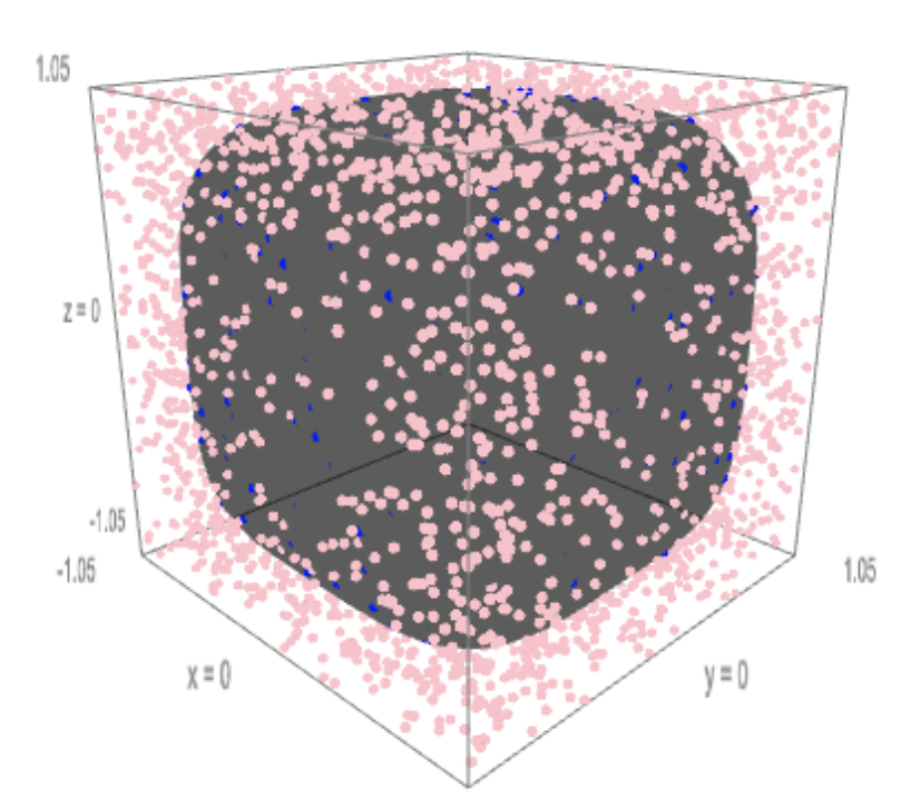
Figure 2: The quartic bounds the convex region consisting of the gray points.

As in Example 0.2.3 with the TV screen, we can get a rough idea of the volume of $S$ by sampling. This is illustrated in Figure 2. Our set $S$ is compact, convex, and contained in the cube given by $-1.05\leq x,y,z\leq 1.05$. We sampled $10000$ points uniformly from that cube. For each sample we checked the sign of $f(x,y,z)$. By multiplying the cube’s volume $(2.1)^{3}=9.261$ by the fraction of the number of gray points and the number of sampled points, Sage found within few seconds that the volume of the quartic body $S$ is $\approx 6.4771$. In order to obtain a higher precision, we now compute the volume of $S$ with the help of $D$-modules.

We use the notation $\text{pr}\colon\mathbb{R}^{3}\to\mathbb{R}$ for the projection onto the $x$-coordinate. Let $v(x)=\text{vol}_{2}\left({\rm pr}^{-1}(x)\cap S\right)$ denote the area of the fiber over any point $x$ in $\mathbb{R}$. We write $e_{1}<e_{2}$ for the two branch points of the map pr restricted to the quartic surface $\{f=0\}$. They can be computed by help of resultants, for instance by the following steps in Singular with the library solve.lib:

ΨLIB "solve.lib";
Ψring r=0,(x,y,z),dp; setring r;
Ψpoly F=x^4+y^4+z^4+x^3*y*1/20-x*y*z*1/20-y*z*1/100+z^2*1/50-1;
Ψdef DFy=diff(F,y); def DFz=diff(F,z);
Ψdef resy=resultant(F,DFy,y); def resz=resultant(F,DFz,z);
Ψideal I=F,resy,resz;
Ψdef A=solve(I); setring A; SOL;
Ψ

The final output SOL is a list of the $36$ roots of the zero-dimensional ideal $I$. The first two of them are real. They are the branch points of pr. We obtain $e_{1}\approx-1.0023512$ and $e_{2}\approx 1.0024985$. By [LMSED19, Theorem 9], the area function $v(x)$ is a period of the rational integral

$$\frac{1}{2\pi i}\oint\frac{y}{f(x,y,z)}\frac{\partial f(x,y,z)}{\partial y}dydz.$$

Set $w(t)=\int_{e_{1}}^{t}v(x)dx$. The desired $3$-dimensional volume is $\text{vol}_{3}(S)=w(e_{2})$.

Using Lairez’ implementation periods in MAGMA, we compute a differential operator $P$ of order eight that annihilates $v(x)$. Again, $P\partial$ then annihilates $w(x)$. One initial condition is $w(e_{1})=0$. We obtain eight further initial conditions $w^{\prime}(x)=\text{vol}_{2}(S_{x})$ for points $x\in(e_{1},e_{2})$ by running the same algorithm for the $2$-dimensional semi-algebraic slices $S_{x}={\rm pr}^{-1}(x)\cap S$. In other words, we make eight subroutine calls to an area measurement as in Example 0.2.3.

From these nine initial conditions we derive linear relations of the coefficients in the local basis expansion at $e_{2}$. These computations are run in Sage as described in steps 1–4 above. We find the approximate volume of our convex body $S$ to be

$$\begin{matrix}\approx 6.43883248057289354474073389596995618895842088923511697626632892312\\ 8826915527388764216209149558398903829431137608893452690352556009760\\ 102417119080476940553482655811421276613538061395975793530527102208\\ 94191557015215864701708740021943845291406868562277595417150971133\\ 9913473405961763289220607208551633239796916338376007073876010731\\ 824775206150471436725046090092340906637773227339039682229623521\\ 496362328661311755793068754414836072122568105348117876005826\\ 4738867105810326818911578448323758536767168707442532146029\\ 753762594261578920477859.\end{matrix}$$

This numerical value is guaranteed to be accurate up to $550$ digits.

0.3 Statistics

In this lecture, we explore the role of $D$-modules in algebraic statistics. Our discussion centers around two themes. First, we study the Bernstein–Sato ideal of the likelihood function of a discrete statistical model. We present a case study that suggests a relationship between that ideal and maximum likelihood estimation. Thereafter, we turn to the holonomic gradient method (HGM) for continuous distributions. This method is the result of collaborations between statisticians and $D$-module experts in Japan. We explain how HGM is used for maximum likelihood estimation. This is implemented in an R package [TKS⁺17].

Let $D_{n}=\mathbb{C}[x_{1},\ldots,x_{n}]\langle\partial_{1},\ldots,\partial_{n}\rangle$ be the $n$th Weyl algebra and adjoin one new formal variable $s$ that commutes with all $x_{i}$ and $\partial_{j}$. This defines the ring $D_{n}[s]$. Fix a polynomial $f\in\mathbb{C}\left[x_{1},\ldots,x_{n}\right]$ and consider the $D_{n}[s]$-module $\mathbb{C}\left[x_{1},\ldots,x_{n},f^{s},f^{-1},s\right]$. Here the action of $D_{n}[s]$ on this module is given by the usual rules of calculus and arithmetic, in particular

$$\partial_{i}\bullet f^{s}\,\,=\,\,s\cdot\frac{\partial f}{\partial x_{i}}\cdot f^{-1}\cdot f^{s}\,\,=\,\,s\cdot\frac{\partial f}{\partial x_{i}}\cdot f^{s-1}.$$

The Bernstein–Sato polynomial of $f$ is the unique monic univariate polynomial $b_{f}\in\mathbb{C}[s]$ of minimal degree such that $P\bullet f^{s+1}=b_{f}\cdot f^{s}$ for some $P\in D[s]$. The polynomial $b_{f}$ was called the global $b$-function in [SST00, Section 5.3], to which we refer for details. It is known that $b_{f}$ is non-zero. M. Kashiwara [Kas76] showed that all its roots are negative rational numbers. The Bernstein–Sato polynomial is computed as the generator of the following principal ideal:

$$\langle b_{f}\rangle\,\,=\,\,\left(\text{Ann}_{D[s]}\left(f^{s}\right)+\langle f\rangle\right)\,\cap\,\mathbb{C}[s].$$

Here, $\,\text{Ann}_{D[s]}\left(f^{s}\right)=\left\{P\in D[s]\mid P\bullet f^{s}=0\right\}\,$ denotes the $s$-parametric annihilator of $f^{s}$. A method for computing this $D[s]$-ideal can be found in [SST00, Algorithm 5.3.15].

We now pass to the case $k\geq 2$ of several polynomials $f_{1},\ldots,f_{k}\in\mathbb{C}\left[x_{1},\ldots,x_{n}\right]$. Following [BvdVWZ19] and the references therein, we define the Bernstein–Sato ideal of the tuple of polynomials $f=(f_{1},\ldots,f_{k})$ as follows:

$$\mathcal{B}\left(f\right)\,\,=\,\,\left(\,\text{Ann}_{D_{n}[s_{1},\ldots,s_{k}]}\left(f_{1}^{s_{1}}\cdots f_{k}^{s_{k}}\,\right)\,+\,\langle f_{1}\cdots f_{k}\rangle\right)\,\cap\,\,\mathbb{C}[s_{1},\ldots,s_{k}].$$ (19)

Here, $s=(s_{1},\ldots,s_{k})$ and the $s$-parametric annihilator of $f^{s}\coloneqq f_{1}^{s_{1}}\cdots f_{k}^{s_{k}}$ is

$$\,\text{Ann}_{D_{n}[s_{1},\ldots,s_{k}]}\left(f^{s}\right)\,\,=\,\,\bigl{\{}P\in D_{n}[s_{1},\ldots,s_{k}]\mid P\bullet f^{s}=0\bigr{\}}.$$

An implementation for performing the computation on the right hand side in (19) is available in the Singular library dmod.lib.

Note that the ideal $\mathcal{B}(f)$ consists of all polynomials $b\in\mathbb{C}[s_{1},\ldots,s_{k}]$ that satisfy

$$\qquad b\cdot\prod_{i=1}^{k}f_{i}^{s_{i}}\,\,=\,\,P\bullet\prod_{i=1}^{k}f_{i}^{s_{i}+1}\quad\hbox{for some $\,P\in D_{n}[s_{1},\ldots,s_{k}]$.}$$

For $k=1$, the ideal $\mathcal{B}(f)$ is generated by the Bernstein–Sato polynomial $b_{f}$. If $k>1$, the Bernstein–Sato ideal is generally not principal. By [BvdVWZ19, Theorem 1.5.1], all the irreducible components of codimension one in the variety of $\mathcal{B}\left(f\right)$ are hyperplanes of the special form

$$a_{1}s_{1}+\ldots+a_{k}s_{k}+b\,=0\,\quad\text{ where }\,\,a_{1},\ldots,a_{k}\in\mathbb{Q}_{\geq 0}\,\,{\rm and}\,\,b\in\mathbb{Q}_{>0}.$$ (20)

This generalizes the fact that the roots of $b_{f}\in\mathbb{C}[s]$ are negative rationals.

We are interested in studying the Bernstein–Sato ideals of parametric statistical models for discrete data. These models are families of probability distributions on $k$ states, where the probability of the $i$th state is given by a polynomial $f_{i}$. The $n$ unknowns $x=(x_{1},\ldots,x_{n})$ represent the parameters of the models. A key feature of any statistical model is the identity

$$f_{1}(x)+f_{2}(x)+\cdots+f_{k}(x)\,\,=\,\,1,$$ (21)

along with the following reasonable semi-algebraic hypothesis:

$$\,\exists\,u\in\mathbb{R}^{n}\,\,\forall\,i\in\{1,\ldots,k\}\,:\,f_{i}(u)>0.$$

The coefficients of $f_{i}$ are usually rational numbers. Here is a familiar example:

[Flipping a biased coin] Let $n=1$ and $m=k-1$, so we can reindex from $0$ to $m$. Set $f_{i}(x)=\binom{m}{i}x^{i}(1-x)^{m-i}\in\mathbb{Q}[x]$ for $i=0,\ldots,m$. Identity (21) holds by the Binomial Theorem. We also set $f^{s}\coloneqq f_{0}^{s_{0}}f_{1}^{s_{1}}\cdots f_{m}^{s_{m}}$. The unknown $x$ represents the bias of the coin, a real number between $0$ and $1$. This is the probability that the coin comes up heads. Then $f_{i}(x)$ is the probability of observing $i$ heads among $m$ independent coin tosses.

The $s$-parametric annihilator $\,\text{Ann}_{D[s]}\left(f^{s}\right)\,$ is the $D[s]$-ideal generated by

$$x(x-1)\partial_{x}\,-\,mx\sum_{j=0}^{m}s_{j}\,+\,\sum_{j=2}^{m}(j-1)s_{j}.$$

This is the result of a computation for small values of $m$. The Bernstein–Sato ideal $\mathcal{B}\left(f\right)\subset\mathbb{Q}[s_{0},\ldots,s_{m}]$ is obtained by adding $f_{0}f_{1}\cdots f_{m}$ to this ideal and then eliminating $x$ and $\partial$. We find that $\mathcal{B}\left(f\right)$ is the principal ideal generated by the following product of linear forms:

$$\!\!\!\!\prod_{j=1}^{\binom{m+1}{2}}\!\!\left(s_{1}+2s_{2}+\cdots+ms_{m}+j\right)\cdot\!\!\prod_{k=1}^{\binom{m+1}{2}}\!\!\left(ms_{0}+(m{-}1)s_{1}+\cdots+s_{m-1}+k\right).$$ (22)

One sees that all factors are linear forms with positive coefficients, as predicted in (20). Note that we can recover these linear factors in a combinatorial way from the following table. The rows mean that $f_{i}$ is a monomial in $x$ and $1-x$, and the columns specify the exponents of these monomials:

	$f_{0}$	$f_{1}$	…	$f_{m-1}$	$f_{m}$	$\sum$
$x\quad$	$0$	$1$	…	$m-1$	$m$	$\binom{m+1}{2}$
$1-x\,$	$m$	$m-1$	…	$1$	$0$	$\binom{m+1}{2}$

The validity of the Formula (22) can be derived from the results on hyperplane arrangements in [Bud15, Section 6]. The point is that, for $n=1$ parameter, each $f_{i}$ is a product of linear forms, by the Fundamental Theorem of Algebra. Hence, $f_{1}f_{2}\cdots f_{k}$ defines an arrangement in $\mathbb{R}^{1}$. The rows of the table indicate the multiplicity of each hyperplane in the product.

In the context of statistics, the $s_{i}$ represent nonnegative integers which summarize an independent and identically distributed sample. Namely, $s_{i}$ is the number of observations of the $i$th outcome. The sum $s_{1}+s_{2}+\cdots+s_{k}$ is the sample size of the experiment. The function $\,f^{s}\,=\,f_{1}^{s_{1}}f_{2}^{s_{2}}\cdots f_{k}^{s_{k}}$ is the likelihood function of the model with respect to the data. We think of $s$ as parameters, so we are interested in the situation when the model is fixed and the data varies. The vector $s$ of counts ranges over $\mathbb{N}^{k}$, or even over $\mathbb{R}^{k}$ or $\mathbb{C}^{k}$, and we treat its coordinates $s_{i}$ as unknowns. The role of the likelihood function $f^{s}$ in statistics can be summarized by referring to the two camps in the history of statistics:

Frequentists: Compute $\,{\rm argmax}(f^{s})$, i.e., solve an optimization problem.

Bayesians:     Compute $\,\int_{\gamma}f^{s}dx$, i.e., evaluate a certain definite integral. We refer to Sullivant’s book [Sul18, Chapter 5] for a discussion of these two perspectives. The integration problem is reminiscent of the volume computation in the previous lecture. Let us now discuss the optimization problem. This is the problem of maximum likelihood estimation (MLE). The aim is to maximize $f^{s}$ over a suitable open subset of parameters $x$ in $\mathbb{R}^{n}$. To address this problem algebraically, one studies the map that associates to $s$ the critical points. This map is an algebraic function. The number of its branches is known as the maximum likelihood degree (ML degree); see [HS14] and [Sul18, Chapter 7]. Models of special interest are those where the ML degree is one. This means that the MLE is given by a rational function. Such models were studied recently in [DMS19]. The following two examples have this property.

[Example 0.3 revisited] Consider the model where a biased coin is flipped $m$ times. The likelihood function $f^{s}$ has its unique critical point at

$$1-\hat{x}\,\,=\,\,\frac{1}{m}\cdot\frac{m\cdot s_{0}+(m-1)\cdot s_{1}+\cdots+1\cdot s_{m-1}+0\cdot s_{m}}{s_{0}+s_{1}+s_{2}+\cdots+s_{m}}.$$

The probability estimates $\,f_{i}(\hat{x})\,$ are alternating products of linear forms in the counts $s_{0},\ldots,s_{m}$. The linear forms appearing in the numerators are seen in (22).

We examine the model that serves as the running example in [DMS19]. It concerns the following simple experiment: Flip a biased coin. If it shows head, then flip it one more time. Here $k=3,\,m=2$ and $n=1$. The model is given algebraically by $\,f_{0}=x^{2}$, $f_{1}=x(1-x)$, and $f_{2}=1-x$. These three polynomials in $\mathbb{Q}[x]$ sum to $1$. The likelihood function equals

$$f^{s}\,\,=\,\,f_{0}^{s_{0}}f_{1}^{s_{1}}f_{2}^{s_{2}}\,\,=\,\,x^{2s_{0}+s_{1}}\cdot(1-x)^{s_{1}+s_{2}}.$$

This is annihilated by the following first-order operator:

$$P\,\,=\,\,(x^{2}-x)\partial\,-\,(2s_{0}+s_{1}+s_{2})x\,+s_{1}+s_{2}\,\in\,D[s_{0},s_{1},s_{2}].$$

By eliminating $x$ and $\partial$ from the $D[s]$-ideal generated by $P$ and $x(1-x)$, we get

$$\mathcal{B}\left(f\right)\,\,=\,\,\biggl{\langle}\,\prod_{k=1}^{3}\left(2s_{0}+s_{1}+k\right)\cdot\prod_{l=1}^{2}\left(s_{1}+s_{2}+l\right)\,\biggr{\rangle}.$$

Thus, the Bernstein–Sato ideal is principal and generated by a product of linear forms (20). As before, we recover the linear factors appearing in $\mathcal{B}(f)$:

	$f_{0}$	$f_{1}$	$f_{2}$	$\sum$
$x$	$2$	$1$	$0$	$3$
$1-x$	$0$	$1$	$1$	$2$

This table of multiplicities mirrors the formula in [DMS19, Example 2] for the maximum likelihood estimate in the coin flip model:

$$\hat{x}\,\,=\,\,\frac{2s_{0}+s_{1}}{2s_{0}+2s_{1}+s_{2}}\,,\qquad 1-\hat{x}\,\,=\,\,\frac{s_{1}+s_{2}}{2s_{0}+2s_{1}+s_{2}}.$$

Just like in Example 0.3, the numerators are precisely the linear factors in $\mathcal{B}(f)$.

Our discussion suggests that there is a deeper connection between $D$-module theory and likelihood geometry [HS14]. This deserves to be explored. Further, it would be interesting to study the Bayesian integrals $\int_{\gamma}f^{s}$ using the $D$-module methods from the previous lecture.

We now come to the Holonomic Gradient Method (HGM). Consider the problem of maximum likelihood estimation in statistics, but now for continuous distributions rather than discrete ones. Our aim is to explain the benefit gained from $D$-module theory. Indeed, many functions of relevance in statistics are holonomic. A key idea is to compute and represent the gradient of such a function from its canonical holonomic representation.

The statistical aim of MLE is to find parameters for which an observed outcome is most probable [Sul18, Chapter 7]. This can be formulated as an optimization problem, namely to maximize the likelihood function. For discrete models, this function has the form $f^{s}$, as seen above. In what follows we consider the likelihood function for continuous models.

Our goal is to find a local maximum of a holonomic function using a variant of gradient descent. For the sake of efficiency, our computations are carried out in the rational Weyl algebra $R=\mathbb{C}(x)\langle\partial\rangle$. See [SST00, Section 1.4] for the theory of Gröbner bases in $R$. Unless otherwise stated, we use the graded reverse lexicographical order $\prec$. For $n=2$, this gives

$$1\prec\partial_{2}\prec\partial_{1}\prec\partial_{2}^{2}\prec\partial_{1}\partial_{2}\prec\partial_{1}^{2}\prec\cdots.$$

Let $f(x_{1},\ldots,x_{n})$ be a real-valued holonomic function and $I$ a $D$-ideal with finite holonomic rank such that $I\bullet f=0$. Thus, $R/RI$ is finite-dimensional over $\mathbb{C}(x_{1},\ldots,x_{n})$. In our application, $f$ will be the likelihood function of a statistical model. Let $\text{rank}(I)=m\in\mathbb{N}_{>0}$. We write $S=\left\{s_{1},\ldots,s_{m}\right\}$, with $s_{1}=1$, for the set of standard monomials for a Gröbner basis of $RI$ in $R$. By Proposition 5, the $m$ entries of the following vector are holonomic functions

$$F\,\,=\,\,\left(s_{1}\bullet f,s_{2}\bullet f,\ldots,s_{m}\bullet f\right)^{T}.$$

Note that the first entry of $F$ is the given function $f$. In symbols, $(F)_{1}=f$. Since the $D$-ideal $I$ has holonomic rank $m$, there exist unique matrices $P_{1},\ldots,P_{n}\in\mathbb{C}(x_{1},\ldots,x_{n})^{m\times m}$ such that

$$\qquad\partial_{i}\bullet F\,\,=\,\,P_{i}\cdot F\qquad\text{for }\,\,i=1,\ldots,n.$$ (23)

The system of linear partial differential equations (23) is called the Pfaffian system of $f$. Note that it depends on the specific $R$-ideal $RI$ and on the chosen term order. The matrices $P_{i}$ can be computed as follows. We apply the division algorithm modulo our Gröbner basis to the operators $\partial_{i}s_{j},$ for $i\in\{1,\ldots,n\}$ and $j\in\{1,\ldots,m\}$. The resulting normal form equals

$$a^{(i)}_{j1}(x)s_{1}\,+\,a^{(i)}_{j2}(x)s_{2}\,+\,\cdots\,+\,a^{(i)}_{jm}(x)s_{m},$$

where the coefficients $a^{(i)}_{jk}$ are rational functions in $x_{1},\ldots,x_{n}$. This means that the operator $\,\partial_{i}s_{j}-\sum_{k=1}^{m}a^{(i)}_{jk}(x)s_{k}\,$ is in the $R$-ideal $RI$. From this one sees that the coefficient $a^{(i)}_{jk}(x)$ is the entry of the $m{\times}m$ matrix $P_{i}$ in row $j$ and column $k$.

We have now reached the following important conclusion. Suppose $x$ is replaced by a point $u$ in $\mathbb{Q}^{n}$. Here $u$ might be a highly accurate floating point representation of a point in $\mathbb{R}^{n}$. The numerical evaluation of the gradient of $f$ at $u$ reduces to multiplying the vector $F(u)\in\mathbb{Q}^{m}$ by matrices $P_{i}(u)$ with explicit rational entries. A tacit assumption made here is that $u$ lies in the complement of the singular locus of the Pfaffian system (23) that encodes $f$.

[$n=1$] Let $f$ be a holonomic function annihilated by

$$I\,\,=\,\,\langle\,x\partial^{3}-(x+1)\partial+1\,\rangle.$$

The generator by itself is a Gröbner basis for $RI$. The set of standard monomials equals $S=\{1,\partial,\partial^{2}\}$, and this is a $\mathbb{C}(x)$-basis of $R/RI$. From $I$ we see that

$$\partial^{3}\bullet f\,\,=\,\,\frac{x+1}{x}\partial\bullet f\,-\,\frac{1}{x}\cdot f.$$

Let $F=(f,\partial\bullet f,\partial^{2}\bullet f)^{T}$. This yields the following Pfaffian system for $f$:

$$\partial\bullet F\,\,=\,\,P\cdot F\quad{\rm where}\quad P\,\,=\,\,\begin{pmatrix}0&1&0\\ 0&0&1\\ -\frac{1}{x}&\frac{x+1}{x}&0\end{pmatrix}.$$

Using notation familiar from calculus, for any non-zero real number $u$ we have

$$\begin{pmatrix}f^{\prime}(u)\\ f^{\prime\prime}(u)\\ f^{\prime\prime\prime}(u)\end{pmatrix}\,\,=\,\,\begin{pmatrix}0&1&0\\ 0&0&1\\ -\frac{1}{u}&\frac{u+1}{u}&0\end{pmatrix}\cdot\begin{pmatrix}f(u)\\ f^{\prime}(u)\\ f^{\prime\prime}(u)\end{pmatrix}.$$

This matrix-vector formula is useful for the design of numerical algorithms.

Given a holonomic function $f$, represented by a holonomic $D$-ideal, we are interested in the following two questions. The first of these was already discussed in the previous lecture.

How to evaluate $f$ at a point with the help of the knowledge of $I$?

How to find local minima of $f$ with the help of the knowledge of $I$? We first describe how to evaluate the holonomic function $f$ at a point $\tilde{x}$ by a first order approximation. Assume we are able to numerically evaluate $f$ at some particular point $x^{(0)}$, depending on the precise situation. Choose a path $x^{(0)}\to x^{(1)}\to\cdots\to x^{(K)}=\tilde{x}$, with $x^{(k+1)}$ sufficiently close to $x^{(k)}$ for all $k=0,\ldots,K-1$ and such that the path does not cross the singular locus of the Pfaffian system of $f$. The following algorithm is referred to as the

Holonomic Gradient Method (HGM).

Compute a Gröbner basis of $RI$ in the rational Weyl algebra $R$.

Compute the set of standard monomials $S$ and the Pfaffian system (23).

Evaluate $F$ at one point $x^{(0)}$ and denote the result by $\bar{F}$. Set $k=0$.

Approximate the value of the vector $F$ at $x^{(k+1)}$ by its first-order Taylor polynomial, and denote the result again by $\bar{F}$:

$$F\left(x^{(k+1)}\right) \,\,\approx\,\,F\left(x^{(k)}\right)\,+\,\sum_{i=1}^{n}\left(x_{i}^{(k+1)}-x_{i}^{(k)}\right)\cdot\left(\partial_{i}\bullet F\right)\left(x^{(k)}\right)$$

$$\,\,=\,\,F\left(x^{(k)}\right)\,+\,\sum_{i=1}^{n}\left(x_{i}^{(k+1)}-x_{i}^{(k)}\right)\cdot P_{i}\left(x^{(k)}\right)\cdot\bar{F}.\vspace{-0.2cm}$$

Increase the value of $k$ by $1$. If $k<K$, return to step 4. Otherwise stop. Steps 1 to 3 need to be carried out only once for $(f,I)$. The output of this algorithm is a vector $\bar{F}$ that approximates $F(\tilde{x})$. The first coordinate of $F(\tilde{x})$ is the desired scalar $f(\tilde{x})$. Hence the first coordinate of $\bar{F}$ is our approximation.

Remark 0.3.1.

To turn the HGM into a practical algorithm, it is essential to incorporate some knowledge from numerical analysis. For instance, there is a lot of freedom in choosing the numerical approximation method in step 4. Nakayama et al. [STT⁺10] use the Runge–Kutta method of fourth order. Another possibility is to use a second order Taylor approximation. Here one computes the Hessian of $f$ also by means of the Pfaffian system of $f$.

Remark 0.3.2.

In practical applications, the Gröbner basis computation in step 1 may not provide results within a reasonable time, but sometimes a partial Gröbner basis for $RI$ suffices to certify holonomicity. From this one gets a finite superset $S$ of the unknown set of true standard monomials. The set $S$ spans $R/RI$, but it may not be linearly independent. In that case, one can still compute a Pfaffian system, but the $P_{i}$ are not necessarily unique anymore. This relaxation might work well in practice.

We are now endowed with all necessary tools for finding a local minimum of the holonomic function $f$. As before, $f$ is encoded by an annihilating $D$-ideal $I$ with finite holonomic rank. This encoding is the input to the next algorithm.

Holonomic Gradient Descent (HGD).

Compute a Gröbner basis of $RI$ in the rational Weyl algebra $R$.

Compute the set of standard monomials $S$ and the Pfaffian system (23).

Numerically evaluate $F(x^{(0)})$ at some starting point $x^{(0)}$ and put $k=0$. Denote this value by $\bar{F}$. The evaluation method is chosen to be adapted to the problem.

For $i=1,\ldots,n$, evaluate the first coordinate of $\,P_{i}(x^{(k)})\bar{F}$. Let $\bar{G}$ be the vector of these $n$ numbers. This approximates the gradient $\nabla f$ at $x^{(k)}$ since

$$\,\partial_{i}\bullet f\,\,=\,\,\left(\partial_{i}\bullet F\right)_{1}\,\,=\,\,\left(P_{i}\cdot F\right)_{1}.$$

If a termination condition of the iteration is satisfied, stop. Otherwise go to step 6.

Put $x^{(k+1)}=x^{(k)}-h_{k}\bar{G}$, where $h_{k}$ is an appropriately chosen step length.

Numerically evaluate $F$ at $x^{(k+1)}$ by step 4 of the HGM and set this value to $\bar{F}$. Increase the value of the index $k$ by one and return to step 4 above.

The algorithm returns a point $x^{(k)}$ along with the value of $F$ at that point. The first entry of this output is a numerical approximation of a local minimum of the holonomic function $f$. Again, one should be aware that, in general, this algorithm works only within connected components contained in the complement of the singular locus of the Pfaffian system of $f$.

In order to develop a practical implementation, and to assess the quality of the method, one needs some expertise from numerical analysis. The choices one makes can make a huge difference. For instance, consider the choice of the step size $h_{k}$. This is a well-studied subject in numerical optimization, and there are various standard recipes for carrying out gradient descent. In current applications to data science, stochastic versions of gradient descent play a major role, and it would be very nice to connect $D$-modules to these developments.

The applicability of HGD arises from the fact that many distributions that are used in practice are given by holonomic functions. One example is the cumulative distribution function of the largest eigenvalue of a Wishart matrix, cf. [HNTT13]. Another relevant holonomic function is the likelihood function of sampling matrices in $\text{SO}(3)$. In what follows we present in detail an example that stood at the beginning of the development of HGM and HGD.

[The Fisher–Bingham distribution [STT⁺10]] Let

$$\,\mathbb{S}^{n}(r)\,\,=\,\,\left\{x\in\mathbb{R}^{n+1}\mid\lVert x\rVert=r\right\}\,$$

denote the $n$-sphere of radius $r$. Let $x\in\mathbb{R}^{(n+1)\times(n+1)}$ be a symmetric matrix and $y\in\mathbb{R}^{n+1}$ a row vector. Let $\lvert dt\rvert$ denote the standard measure on $\mathbb{S}^{n}(r)$. The Fisher–Bingham integral is

$$F(x,y,r)\,\,=\,\,\int_{\mathbb{S}^{n}(r)}\!\!\exp\left(t^{T}xt+yt\right)|dt|.$$

This is a function in $\binom{n+1}{2}+(n+1)+1$ unknowns, since $x_{kl}=x_{lk}$. It is shown in [STT⁺10, Theorem 1] that the function $F(x,y,r)$ is holonomic. More precisely, the following operators annihilate the Fisher–Bingham integral and generate a $D$-ideal of finite holonomic rank:

$$\sum_{i=1}^{n+1}\partial_{x_{ii}}-r^{2}\,,\quad r\partial_{r}-2\sum_{i\leq j}x_{ij}\partial_{x_{ij}}-\sum_{i}y_{i}\partial_{y_{i}}-n\,,\quad\partial_{x_{ij}}-\partial_{y_{i}}\partial_{y_{j}}\,\,\,{\rm for}\,\,\,i\leq j,\vskip 3.0pt plus 1.0pt minus 1.0pt$$

$$x_{ij}\partial_{x_{ii}}+2(x_{ji}-x_{ii})\partial_{x_{ij}}-x_{ij}\partial_{x_{jj}}+\sum_{k\neq i,j}(x_{jk}\partial_{x_{ik}}-x_{ik}\partial_{x_{jk}})+y_{j}\partial_{y_{i}}-y_{i}\partial_{y_{j}},$$

where $i<j$ in the second line. For a proof, see [STT⁺10, Theorems 2,3]. For $n=1,2$, these operators generate a holonomic $D$-ideal, see [STT⁺10, Proposition 1]. We now define the Fisher–Bingham distribution on the unit sphere $\mathbb{S}^{n}(1)$. This depends on the parameters $x,y$ and has probability density function

$$p(t\!\mid\!x,y)\,\,\,=\,\,\,F(x,y,1)^{-1}\cdot\exp(t^{T}xt+yt).$$

In other words, the Fisher–Bingham distribution plays the role of the Gaussian distribution on the sphere, and the Fisher–Bingham integral $F(x,y,1)$ is its normalizing constant.

We now explain the inference problem to be solved. Let $\{t(1),\ldots,t(N)\}$ be an independent and identically distributed sample of size $N$ drawn from the unit sphere $\mathbb{S}^{n}(1)$. The statistical aim is to estimate the parameters $x=(x_{ij})$ and $y=(y_{i})$ from the given sample. The standard method to do so is MLE. We seek to maximize the likelihood function

$$(x,y)\,\,\mapsto\,\,\prod_{\nu=1}^{N}p(t(\nu)\!\mid\!x,y).$$

For the Fisher–Bingham model, this is equivalent to minimizing the function

$$F(x,y,1)\cdot\exp\left(-\!\!\sum_{1\leq i\leq j\leq{n+1}}S_{ij}x_{ij}\,\,-\sum_{1\leq i\leq{n+1}}S_{i}y_{i}\right).$$ (24)

Here the quantities $S_{i}$ and $S_{ij}$ are real constants that are easily computed from the sample points $t(i)$. Namely, they are the coordinates of the sample mean and the sample covariance matrix:

$$S_{i}\,=\,N^{-1}\sum_{\nu=1}^{N}t_{i}(\nu)\quad{\rm and}\quad S_{ij}\,=\,N^{-1}\sum_{\nu=1}^{N}t_{i}(\nu)t_{j}(\nu).$$

The function (24) is a product of two holonomic functions. Hence, it is a holonomic function in the unknowns $x=(x_{ij})$ and $y=(y_{i})$. Furthermore, since our model is an exponential family, the logarithm of (24) is a convex function. This means that a local minimum is already a global one. Our task is therefore to find a local minimum of (24) using HGD.

The authors of [STT⁺10] present two specific data sets and they demonstrate the use of HGD for this input. The data and some code in the computer algebra system Risa/Asir are provided at the website

http://www.math.kobe-u.ac.jp/OpenXM/Math/Fisher-Bingham/.

One of the data sets is the following “astronomical data”. Here $n=2$ and

$$S_{1}=-0.0063, S_{11} =0.3199, S_{22} =0.3605,$$

$$S_{2}=-0.0054, S_{12} =0.0292, S_{23} =0.0462,$$

$$S_{3}=-0.0762, S_{13} =0.0707, S_{33} =0.3276.$$

The starting point is found by minimizing with a quadratic approximation of $F(x,y,1)$, with step size set at $0.05$. Running the HGD revealed the minimum objective function value $\approx 11.6857$. The maximum likelihood parameters are

$$x\,=\,\begin{pmatrix}-0.161&0.3377/2&1.1104/2\\ 0.3377/2&0.2538&0.6424/2\\ 1.1104/2&0.6424/2&-0.0928\end{pmatrix},\quad y\,=\,(-0.019,-0.0162,-0.2286).$$

We reproduced this result, but this did take some effort.

In conclusion, we have argued that holonomic functions arise in many contexts, notably in geometry and statistics. The manipulation of these functions can be done by algorithms from the theory of $D$-modules. Implementations already exist, and they are available in a wide range of computer algebra systems. While the further development of the symbolic computation tools is important, a significant new opportunity lies in advancing the connection to numerical algebraic geometry. Efficient numerical methods for $D$-modules and holonomic functions have a clear potential for future impact in scientific computing and data science. These lectures offered a very first glimpse at the underlying mathematics.

Problems

In this section, we offer some ideas for hands-on activities. These were discussed in an afternoon session during the Berlin school. The items range from easy exercises to challenging questions that suggest research projects. We leave it to our readers to decide which is which. Some hints and solutions are found below.

Let $M$ be a $D$-module which is finite-dimensional as a $\mathbb{C}$-vector space. Show that $M=0$. Hint: Can the commutator of two $n\times n$ matrices be the identity matrix?

Find bases of solutions for the following three second-order linear differential equations:

$$xf^{\prime\prime}+f^{\prime}\,=\,0\quad{\rm and}\quad g^{\prime\prime}\,=\,4x^{2}g\quad{\rm and}\quad x^{2}h^{\prime\prime}-3xh^{\prime}+4h\,=\,0.$$

For each of the following three functions $u,v,w$ in one variable $x$, find a linear ordinary differential equation with polynomial coefficients that is satisfied by that function:

$$u(x)\,=\,x^{3/5}\cdot{\rm log}(x)^{2},\quad v(x)\,=\,{\rm sin}(x)^{5},\quad w(x)\,=\,(1+x^{4})\cdot{\rm exp}(x).$$

A $\mathbb{C}$-basis of the Weyl algebra $D=\mathbb{C}\left[x_{1},\ldots,x_{n}\right]\langle\partial_{1},\ldots,\partial_{n}\rangle$ consists of the normal monomials $x^{a}\partial^{b}$, where $a,b\in\mathbb{N}^{n}$. Find the formula for expressing the operator $\partial^{b}x^{a}$ in that basis.

Let $n=3$. Compute the distraction $\,\widetilde{I}\,$ in $\mathbb{C}[\theta_{1},\theta_{2},\theta_{3}]$ of the $D$-ideal

$$I\,\,=\,\,\langle\partial_{1}^{4},\partial_{2}^{4},\partial_{3}^{4},\partial_{1}\partial_{2}^{2}\partial_{3}^{3},\partial_{1}^{2}\partial_{2}^{3}\partial_{3},\partial_{1}^{3}\partial_{2}\partial_{3}^{2}\rangle.$$

Also, find a $\mathbb{C}$-basis for the vector space $\,{\rm Sol}(I)={\rm Sol}(\widetilde{I})$.

Find a canonical holonomic representation for the bivariate function

$$f(x,y)\,\,=\,\,e^{x\cdot y}\cdot{\rm sin}\frac{y}{1+y^{2}}.$$

Using the integration ideal as in Definition 7, find an operator in $D_{1}$ that annihilates the following function in one variable:

$$\qquad F(x)\,\,=\,\,\int_{0}^{+\infty}\!\!f(x,y)dy,\qquad\text{where $f$ is the function in Problem 6.}$$

Construct a rational function $r$ by taking the ratio of your two favorite polynomials in two variables. Compute $I=\text{Ann}_{D}(r)$ and determine the singular locus ${\rm Sing}(I)\subset\mathbb{C}^{2}$.

Let $f$ be a holonomic function in one variable. Prove that its reciprocal$1/f$ is holonomic if and only if the logarithmic derivative $f^{\prime}/f$ is an algebraic function.

For those who like sheaves: Why is a vector bundle together with a flat connection a module over the sheaf $\mathcal{D}$? Actually, what are these objects over the projective line $\mathbb{P}^{1}$?

For those who like toric geometry: Pick your favorite projective toric manifold and write the presentation ideal (Stanley–Reisner plus linear forms) of its Chow ring in $\mathbb{C}[\partial_{1},\ldots,\partial_{n}]$ and also in $\mathbb{C}[\theta_{1},\ldots,\theta_{n}]$. Determine the solution spaces in both cases.

For those who like the Hodge theory of matroids: Pick your favorite matroid and write the presentation ideal (Stanley–Reisner plus linear forms) of its Chow ring in $\mathbb{C}[\partial_{1},\ldots,\partial_{n}]$ and also in $\mathbb{C}[\theta_{1},\ldots,\theta_{n}]$. Determine the solution spaces in both cases.

Stafford’s Theorem states that every $D$-ideal can be generated by two elements. Let $n=4$ and identify two differential operators that generate the $D$-ideal $\langle\partial_{1},\partial_{2},\partial_{3},\partial_{4}\rangle$. Then, do the same for the $D$-ideal $I$ in Example 5, for some choices of $a,b,c\in\mathbb{Z}$.

Consider the general algebraic equation of degree five in one variable:

$$x_{5}t^{5}+x_{4}t^{4}+x_{3}t^{3}+x_{2}t^{2}+x_{1}t+x_{0}\,\,=\,\,0.$$

Write the roots $t_{1},\ldots,t_{5}$ as a holonomic function of the coefficients $x_{i}$. Restrict your holonomic system to a two-dimensional linear subspace in the $\mathbb{C}^{6}$ of coefficients.

Let $f,g,h$ be as in Problem 2. According to Proposition 3, the functions $fg,\,fh,\,gh,\,f{+}g,\,f{+}h,\,g{+}h$ are holonomic. Find operators in $D_{1}$ that annihilate these functions.

Compute a Gröbner basis in $R$ for the annihilator of the function $f(x,y)$ in Problem 6. Determine the Pfaffian system (23). Verify that $P_{1}$ and $P_{2}$ satisfy [SST00, Equation (1.35)].

Write the likelihood function $f^{s}$ for the random censoring model in [Sul18, Example 7.1.5]. Compute the $s$-parametric annihilator ${\rm Ann}_{D[s]}(f^{s})$ and the Bernstein–Sato ideal $\mathcal{B}(f)$.

Let $n=4$ and let $I$ be the left ideal in $D_{4}$ generated by the four operators

$$3x_{1}\partial_{1}+2x_{2}\partial_{2}+x_{3}\partial_{3}-3, \quad x_{1}\partial_{2}+2x_{2}\partial_{3}+3x_{3}\partial_{4},$$

$$(3x_{2}\partial_{1}+2x_{3}\partial_{2}+x_{4}\partial_{3})^{4}, \quad x_{2}\partial_{2}+2x_{3}\partial_{3}+3x_{4}\partial_{4}.$$

Show that $I$ is holonomic and determine its rank. Compute the characteristic variety and the singular locus. Explain their irreducible components.

Let $n=9$, where the Weyl algebra generators $x_{ij}$ and $\partial_{ij}$ are entries of $3\times 3$ matrices respectively. Let $P$ be the prime ideal in $\mathbb{C}[x_{ij}]$ that defines the group ${\rm SO}(3)$ in $\mathbb{C}^{3\times 3}$. Let $I$ be the $D$-ideal generated by $P$ and

$$\biggl{\{}\,\sum_{k=1}^{3}\,(x_{ki}\partial_{kj}-x_{kj}\partial_{ki})\,\,:\,\,1\leq i<j\leq 3\,\biggr{\}}.$$

Show that $I$ is holonomic and Weyl-closed. Compute its rank and characteristic variety.

Solutions and Hints

Let $M\in\text{Mod}(D)$ with $\dim_{\mathbb{C}}M=m$. Since $[\partial_{i},x_{i}]=\text{id}_{M}$, the trace of the commutator is given by $\text{tr}\left([\partial_{i},x_{i}]\right)=m\cdot 1$. On the other hand, $\partial_{i},x_{i}\in\text{End}_{\mathbb{C}}(M)$ are described by matrices $P_{i},X_{i}\in\mathbb{C}^{m\times m}$. Hence, $\text{tr}\left([\partial_{i},x_{i}]\right)=\text{tr}\left(P_{i}X_{i}-X_{i}P_{i}\right)=\text{tr}(P_{i}X_{i})-\text{tr}\left(X_{i}P_{i}\right)=0$ and therefore $m=0$.

We start with $P_{f}=x\partial^{2}+\partial$ and $I_{f}=\langle P_{f}\rangle$. A computation shows that $\text{in}_{(-w,w)}(I_{f})=I_{f}$ for all $w\in\mathbb{R}^{n}$. Therefore, $I_{f}$ is torus-fixed and $\text{Sol}(I_{f})=\text{Sol}\left(\widetilde{I_{f}}\right)$, where $\widetilde{I_{f}}=\langle\theta^{2}\rangle$. Therefore, $\text{Sol}(I_{f})=\mathbb{C}\left\{1,\log(x)\right\}$.

The second ODE corresponds to the operator $P_{g}=\partial^{2}-4x^{2}$. The lowest order terms of the solutions to $P_{g}$ can be computed by Proposition 8.

Denote by $P_{h}=x^{2}\partial^{2}-3x\partial+4$. We observe that the ideal generated by $P_{h}=\theta^{2}-4\theta+4=(\theta-2)^{2}$ is a Frobenius ideal. The inverse system at $2$ is $\,Q_{2}^{\perp}=\mathbb{C}\{1,x\}$. By Theorem 11, we get $\text{Sol}\left(\langle P_{h}\rangle\right)=\mathbb{C}\left\{x^{2},x^{2}\log(x)\right\}$.

One can reproduce these results by the following Mathematica code:

ΨDSolve[x*y’’[x] + y’[x] == 0, y[x], x]
ΨDSolve[y’’[x] - 4*x^2*y[x] == 0, y[x], x]
ΨDSolve[x^2*y’’[x] - 3*x*y’[x] + 4*y[x] == 0, y[x], x]
Ψ

The reader is encouraged to compute the derivatives and then identify a relation between them. Alternatively, the following code in Mathematica computes annihilating differential operators for $u,v,w$:

Ψ<< RISC‘HolonomicFunctions‘
Ψu = x^(3/5)*(Log[x])^2
Ψannu = Annihilator[u, Der[x]]
Ψv = (Sin[x])^5
Ψannv = Annihilator[v, Der[x]]
Ψw = (1 + x^4)*Exp[x]
Ψannw = Annihilator[w, Der[x]]
Ψ

Start with $n=1$ and then extend. For any nonnegative integers $a$ and $b$,

$$\partial^{b}x^{a}\,\,=\,\,\sum_{i\geq 0}\frac{a!b!}{i!(a-i)!(b-i)!}x^{a-i}\partial^{b-i},$$

where negative powers are $0$ and zero powers are $1$.

Similar to Example 10, consider the staircase under the monomial ideal. This is the cover picture of a text book by Ezra Miller and Bernd Sturmfels.

The following code in Mathematica computes an annihilating ideal for $f$:

Ψ<< RISC‘HolonomicFunctions‘
Ψf = Exp[x*y]*Sin[y*1/(1+y^2)]
Ψann = Annihilator[f,{Der[x],Der[y]}]
Ψ

We find that the operators $\partial_{x}-y$ and $(y^{10}{+}3y^{8}{+}2y^{6}{-}2y^{4}{-}3y^{2}{-}1)\partial_{y}^{2}$ $+({-}2xy^{10}{-}6xy^{8}{-}4xy^{6}{+}4xy^{4}{+}6xy^{2}{+}2x{+}2y^{9}{-}12y^{5}{-}16y^{3}{-}6y)\partial_{y}{+}(x^{2}y^{10}$ $+3x^{2}y^{8}{+}2x^{2}y^{6}{-}2x^{2}y^{4}{-}3x^{2}y^{2}{-}x^{2}{-}2xy^{9}{+}12xy^{5}{+}16xy^{3}{+}6xy{+}y^{6}{-}3y^{4}$ $+3y^{2}{-}1)$ annihilate $f$. It remains to specify sufficiently many initial conditions and to prove that these two operators generate a holonomic $D$-ideal.

The theoretical argument is similar to that in the proof of Proposition 6. For the computation we can use the commands CreativeTelescoping and ApplyOreOperator of the HolonomicFunctions package in Mathematica.

Let $r=p/q$ with $p=x^{2}+xy,\,q=y^{2}\in\mathbb{C}[x,y]$. Running the following code in Singular, using the libraries [AL14, And15, LMM15], solves the problem:

ΨLIB "dmod.lib";ΨLIB "dmodapp.lib";ΨLIB "dmodloc.lib";
Ψring r=0,(x,y),dp; setring r;
Ψpoly p=x^2+x*y;Ψpoly q=y^2;
Ψdef an=annRat(p,q); setring an; LD;
ΨisHolonomic(LD);
ΨDsingularLocus(LD);
Ψdef CV=charVariety(LD); setring CV;
ΨcharVar;
Ψ

For a proof, we refer to the article [HS85] of Harris and Sibuya.

Vector bundles with flat connection over $\mathbb{P}^{1}$ correspond to those over $\mathbb{P}^{\text{an}}$. By the Riemann–Hilbert correspondence, such a vector bundle is determined by its monodromy data. Since the Riemann sphere is simply connected, it follows that vector bundles with flat connection on $\mathbb{P}^{1}$ are classified by globally free sheaves of finite rank with the natural action of $\mathcal{D}$.

We consider the Hirzebruch surface whose Chow ring has the presentation ideal $\,I\,=\,\langle\partial_{1}\partial_{3},\partial_{2}\partial_{4},\partial_{1}+2\partial_{2}-\partial_{3},\partial_{2}-\partial_{4}\rangle$. Then the solution space is

$${\rm Sol}(I)\,\,=\,\,\mathbb{C}\bigl{\{}-x_{1}^{2}+x_{1}x_{2}+x_{1}x_{4}+x_{2}x_{3}+x_{3}^{2}+x_{3}x_{4},\,x_{1}+x_{3},\,x_{2}+2x_{3}+x_{4},\,1\,\bigr{\}}.$$

The quadratic form is the volume polynomial [SST00, Remark 3.6.14] which generates ${\rm Sol}(I)\simeq\mathbb{C}^{4}$ as a cyclic module over $\mathbb{C}[\partial_{1},\partial_{2},\partial_{3},\partial_{4}]$. If we replace each $\partial_{i}$ by $\theta_{i}=x_{i}\partial_{i}$, then the solution space is the same but with each variable $x_{i}$ replaced by the corresponding logarithm ${\rm log}(x_{i})$.

We refer to [Eur20, Definition 1.1] for Chow rings of matroids. Again, the ideal is generated by squarefree monomials and linear forms. Eur [Eur20] gives an explicit formula for the volume polynomial. Just like in the toric case, this polynomial generates the solution space as a $\mathbb{C}[\partial]$-module.

The following code in Macaulay2 computes two generators, which are guaranteed to generate the given ideal $I$ over the rational Weyl algebra.

ΨloadPackage "Dmodules"
ΨD=QQ[x1,x2,x3,x4,d1,d2,d3,d4,
ΨWeylAlgebra=>{x1=>d1,x2=>d2,x3=>d3,x4=>d4}];
ΨD
ΨI=ideal(d1,d2,d3,d4)
Ψstafford I
Ψ

By computing reduced Gröbner bases over $D_{4}$, one then can check that the two obtained operators indeed generate $I$ as a left module over $D_{4}$. We invite our readers to tackle the challenge of computing two generators for the $D$-ideal $I$ in Example 5, for some choices of $a,b,c\in\mathbb{Z}$.

Let $f(t,x_{0},\ldots,x_{5})=x_{5}t^{5}+x_{4}t^{4}+x_{3}t^{3}+x_{2}t^{2}+x_{1}t+x_{0}$. The five roots are algebraic functions $t_{1},\ldots,t_{5}$ in the six variables $x_{0},\ldots,x_{5}$. Let $t$ be one out of these five functions. We have $t(\lambda x_{0},\ldots,\lambda x_{5})=t(x_{0},\ldots,x_{5})$ since $f$ and $\lambda f$ have the same roots. By taking the derivative with respect to $\lambda$, we see that $\theta_{0}+\cdots+\theta_{5}$ annihilates $t$, where $\theta_{k}=x_{k}\partial_{k}$. We similarly observe $t(x_{0},\lambda,x_{1},\ldots,\lambda^{5}x_{5})=\lambda\cdot t(x_{0},\ldots,x_{5})$, which implies that $1-\theta_{1}-2\theta_{2}-\cdots-5\theta_{5}$ annihilates $t$. Now, consider $t$ as a simple root of the holomorphic function $f$. By the Residue Theorem from complex analysis,

$$t\,\,=\,\,\int_{\gamma}\frac{zf^{\prime}}{f}dz$$

for a suitable integration cycle $\gamma$ in the complex plane. From this integral representation, with the help of $A$-hypergeometric series, it follows that

$$\left\{\partial_{i}\partial_{j}-\partial_{k}\partial_{l}\mid i+j=k+l\right\}\,\subseteq\,\text{Ann}_{D_{6}}(t).$$

We refer the reader to [Stu00] for details. See also the opening section in [SST00]. We note that the package HolonomicFunctions in Mathematica is able compute an annihilator of an algebraic function, which is implicitly given. The restriction of this ideal to a two-dimensional linear subspace in the six-dimensional space of coefficients can be run in Singular using the command restrictionIdeal in the library dmoddapp.lib [AL14].

For a recipe, see the proof of Proposition 3. Alternatively, the commands DFinitePlus and DFiniteTimes in the Mathematica package Holonomic Functions compute the annihilators of the sum and product of functions, taking only the annihilators of the single functions as an input.

For computing the Pfaffian system, we recommend using the commands OreGroebnerBasis and OreReduce for Gröbner basis computations in the rational Weyl algebra. They belong to the package HolonomicFunctions in Mathematica. Do verify that $P_{1}$ and $P_{2}$ satisfy [SST00, Equation (1.35)].

Fix $n=3$ and $k=4$. The random censoring model is parametrized by

$$\begin{matrix}f_{1}\,=\,\frac{x_{3}}{x_{1}+x_{2}+x_{3}},&\quad&f_{2}\,=\,\frac{x_{1}x_{3}}{(x_{2}+x_{3})(x_{1}+x_{2}+x_{3})},\vskip 3.0pt plus 1.0pt minus 1.0pt\\ f_{3}=\frac{x_{2}x_{3}}{(x_{1}+x_{3})(x_{1}+x_{2}+x_{3})},&\quad&f_{4}=\frac{x_{1}x_{2}(x_{1}+x_{2}+2x_{3})}{(x_{1}+x_{3})(x_{2}+x_{3})(x_{1}+x_{2}+x_{3})}.\end{matrix}$$

Geometrically, this statistical model is the cubic surface $\{2f_{1}f_{2}f_{3}+f_{2}^{2}f_{3}+f_{2}f_{3}^{2}-f_{1}^{2}f_{4}+f_{2}f_{3}f_{4}=0\}$ inside the tetrahedron $\{f_{1}+f_{2}+f_{3}+f_{4}=1\}$. Its likelihood function is $f^{s}=f_{1}^{s_{1}}f_{2}^{s_{2}}f_{3}^{s_{3}}f_{4}^{s_{4}}$. To compute $\,\text{Ann}_{D[s]}\left(f^{s}\right)$, we must adapt [SST00, Algorithm 5.3.15] to the case of rational functions.

We provide the following code in Singular, in order to solve this exercise.

ΨLIB "dmod.lib"; LIB "dmodapp.lib";
ΨLIB "dmodloc.lib"; LIB "primdec.lib";
Ψint n=4; def D=makeWeyl(n); setring D;
Ψideal I=3*x(1)*D(1)+2*x(2)*D(2)+x(3)*D(3)-3,
Ψ(3*x(2)*D(1)+2*x(3)*D(2)+x(4)*D(3))^4,
Ψx(1)*D(2)+2*x(2)*D(3)+3*x(3)*D(4),
Ψx(2)*D(2)+2*x(3)*D(3)+3*x(4)*D(4);
ΨisHolonomic(I);
ΨDsingularLocus(I);
Ψdef CV = charVariety(I); setring CV;
ΨcharVar;
Ψlist pr=minAssGTZ(charVar);Ψpr;
Ψ

For the $\text{SO}(2)$ case, computations can be easily run using a computer algebra software. For the $\text{SO}(3)$ case, computations get highly intensive. We refer the reader to an article of Koyama [Koy19]. Let us draw the reader’s attention to the following lemma of this article. Let $I$ be a holonomic $D$-ideal. If $\,\text{in}_{(0,e)}(I)\,$ is prime, then $I$ is maximal. This statement may be used in order to investigate if a holonomic ideal contained in the annihilator of a function already presents the full annihilator. The rank computation for the $\text{SO}(3)$ case is carried out in the article [ALSS19] by investigating the holonomic dual of that $D$-ideal. Moreover, a generalization to compact Lie groups other than $\text{SO}(n)$ can be found therein.

Acknowledgments. A number of people helped us with the material presented here. We are grateful to Michael F. Adamer, Paul Görlach, Alexander Heaton, Roser Homs Pons, Christoph Koutschan, Christian Lehn, Viktor Levandovskyy, András C. Lőrincz, Marc Mezzarobba, and Emre C. Sertöz.

After-effects. We are happy to report that our lecture notes, made available in first version on the arXiv in October 2019, had some productive consequences already. One of these is our article [ALSS19]. Andreas Bernig applied the theory of holonomic functions for completing his proof of a conjecture by Joe Fu, establishing a link between integral geometry and combinatorics. Together with Robin van der Veer, we are currently working on a better structural understanding of the connection between Bernstein–Sato theory and MLE in statistics.

References

- [AL14] Daniel Andres and Viktor Levandovskyy. dmodapp.lib: A Singular 4-1-2 library for applications of algebraic D-modules, 2014.
- [ALSS19] Michael F. Adamer, András C. Lőrincz, Anna-Laura Sattelberger, and Bernd Sturmfels. Algebraic analysis of rotation data. arXiv:1912.00396, 2019.
- [And15] Daniel Andres. dmodloc.lib: A Singular 4-1-2 library for localization of algebraic D-modules and applications, 2015.
- [Bud15] Nero Budur. Bernstein–Sato ideals and local systems. Annales de l’Institut Fourier, 65(2):549–603, 2015.
- [BvdVWZ19] Nero Budur, Robin van der Veer, Lei Wu, and Peng Zhou. Zero loci of Bernstein–Sato ideals. arXiv:1907.04010, 2019.
- [DMS19] Eliana Duarte, Orlando Marigliano, and Bernd Sturmfels. Discrete statistical models with rational maximum likelihood estimator. arXiv:1903.06110, 2019.
- [Eur20] Christopher Eur. Divisors on matroids and their volumes. Journal of Combinatorial Theory. Series A, 169:105135, 31, 2020.
- [GLS] Paul Görlach, Christian Lehn, and Anna-Laura Sattelberger. Algebraic analysis of the hypergeometric function of a matrix argument. In preparation.
- [HNTT13] Hiroki Hashiguchi, Yasuhide Numata, Nobuki Takayama, and Akimichi Takemura. The holonomic gradient method for the distribution function of the largest root of a Wishart matrix. Journal of Multivariate Analysis, 117:296–312, 2013.
- [HS85] William A. Harris and Yasutaka Sibuya. The reciprocals of solutions of linear ordinary differential equations. Advances in Mathematics, 58(2):119–132, 1985.
- [HS14] June Huh and Bernd Sturmfels. Likelihood geometry. In Aldo Conca, Sandra Di Rocco, Jan Draisma, June Huh, Bernd Sturmfels, and Filippo Viviani, editors, Combinatorial algebraic geometry : lecture notes from the CIME-CIRM summer school held in Levico Terme, June 10-15, 2013, volume 2108 of Lecture notes in mathematics, pages 63–117. Springer, New York, 2014.
- [HTT08] Ryoshi Hotta, Kiyoshi Takeuchi, and Toshiyuki Tanisaki. D-modules, perverse sheaves, and representation theory, volume 236 of Progress in Mathematics. Birkhäuser Boston, 2008. Translated from the 1995 Japanese edition by Takeuchi.
- [JJK15] Maximilian Jaroschek, Fredrik Johansson, and Manuel Kauers. Ore polynomials in Sage. In Computer Algebra and Polynomials, Lectures notes in Computer Science, pages 105–125. Springer LNCS 8942, 2015.
- [Kas76] Masaki Kashiwara. B-functions and holonomic systems. Rationality of roots of b-functions. Inventiones mathematicae, 38:33–54, 1976.
- [Kou10] Christoph Koutschan. HolonomicFunctions (user’s guide). Technical Report 10-01, RISC Report Series, Johannes Kepler University, Linz, Austria, 2010.
- [Koy19] Tamio Koyama. The annihilating ideal of the Fisher integral. arXiv:1503.05261, 2019.
- [Lai16] Pierre Lairez. Computing periods of rational integrals. Mathematics of Computation, 85:1719–1752, 2016.
- [LMM15] Viktor Levandovskyy and Jorge Martín-Morales. dmod.lib: A singular 4-1-2 library for algorithms for algebraic D-modules, 2015.
- [LMSED19] Pierre Lairez, Marc Mezzarobba, and Mohab Safey El Din. Computing the volume of compact semi-algebraic sets. In Proceedings of the 2019 on International Symposium on Symbolic and Algebraic Computation, ISSAC ’19, pages 259–266, New York, NY, USA, 2019. ACM.
- [LT] Anton Leykin and Harrison Tsai. Dmodules: functions for computations with D-modules. Version 1.4.0.1. A Macaulay2 package available at https://github.com/Macaulay2/M2/tree/master/M2/Macaulay2/packages.
- [MS15] Diane Maclagan and Bernd Sturmfels. Introduction to tropical geometry, volume 161 of Graduate studies in mathematics. American Mathematical Society, Providence, R.I., 2015.
- [SKK73] Mikio Sato, Takahiro Kawai, and Masaki Kashiwara. Microfunctions and pseudodifferential equations. In Hyperfunctions and Pseudo-Differential Equations, volume 6 of Lecture Notes in Mathematics, pages 264–524. Springer, 1973.
- [SST00] Mutsumi Saito, Bernd Sturmfels, and Nobuki Takayama. Gröbner deformations of hypergeometric differential equations, volume 6 of Algorithms and Computation in Mathematics. Springer-Verlag, Berlin, 2000.
- [Sta78] John T. Stafford. Module structure of Weyl algebras. Journal of the London Mathematical Society, s2-18(3):429–442, 1978.
- [Sta80] Richard P. Stanley. Differentiably finite power series. European Journal of Combinatorics, 1(2):75–188, 1980.
- [STT+10] Tomonari Sei, Nobuki Takayama, Akimichi Takemura, Hiromasa Nakayama, Kenta Nishiyama, Masayuki Noro, and Katsuyoshi Ohara. Holonomic gradient descent and its application to Fisher–Bingham integral. Advances in Applied Mathematics, 47, 2010.
- [Stu00] Bernd Sturmfels. Solving algebraic equations in terms of A-hypergeometric series. Discrete Mathematics, 210(1-3):171–181, 2000.
- [Stu02] Bernd Sturmfels. Solving systems of polynomial equations, volume 97 of CBMS regional conference series in mathematics. American Mathematical Society, Providence, R.I., 2002.
- [Sul18] Seth Sullivant. Algebraic statistics. volume 194 of Graduate Studies in Mathematics. American Mathematical Society, Providence, R.I., 2018.
- [Tak92] Nobuki Takayama. An approach to the zero recognition problem by Buchberger algorithm. Journal of Symbolic Computation, 14(2):265 –282, 1992.
- [Tak13] Nobuki Takayama. Gröbner basis for rings of differential operators and applications. In Gröbner Bases: Statistics and Software Systems, pages 279–344, 2013.
- [TKS+17] Nobuki Takayama, Tamio Koyama, Tomonari Sei, Hiromasa Nakayama, and Kenta Nishiyama. hgm: Holonomic Gradient Method and Gradient Descent, 2017. R package version 1.17.
- [Zei90] Doron Zeilberger. A holonomic systems approach to special functions identities. Journal of Computational and Applied Mathematics, 32(3):321–368, 1990.