On some spectral properties of stochastic similarity matrices for data clustering
Abstract.
Clustering in image analysis is a central technique that allows to classify elements of an image. We expand upon recent results in spectral analysis for Gaussian mixture distributions, and in particular, provide conditions for the existence of a spectral gap between the leading and remaining eigenvalues for matrices with entries from a Gaussian mixture with two real univariate components. Furthermore, we describe an algorithm in which a collection of image elements is treated as a dynamical system in which the existence of the mentioned spectral gap results in an efficient clustering.
Contents
1 Preliminaries
1.1 Contraction mappings1.2 Reproducing kernel space1.3 Kernel matrix and kernel operator1.4 Eigenvalues1.5 Mixture distributions1.6 Gaussian components1.7 Multivariate Gaussian distribution
2 Estimates on the second eigenvalue of a Gaussian mixture
3 Clustering and simulations
3.1 Single component in ℝ ℝ \mathbb{R} 3.2 Mixture of two components in ℝ ℝ \mathbb{R} 3.3 Single component in ℝ 2 superscript ℝ 2 \mathbb{R}^{2} 3.4 Mixture of two components in ℝ 2 superscript ℝ 2 \mathbb{R}^{2} 3.5 Clustering of lines or shapes3.6 Mixture of two components in ℝ ℝ \mathbb{R}
4 Example of the main theorem5 Conclusions and further work6 Appendix
The common feature of modern data analysis is the large amount of data which collectively have a very high dimension. High dimensionality hinders data processing, and, specifically, data clustering.
However, high dimensionality is quite often caused by data representation, while the number of parameters needed to accurately describe the data is much smaller.
Dimensionality reduction of large data sets can be achieved by treating a collection of elements in a set as a dynamical system. For example, if a data set is an image, then, initially, each element of the image may be assigned a spacial coordinate in ℝ m superscript ℝ 𝑚 \mathbb{R}^{m} m 𝑚 m 2 2 2 3 3 3 n 𝑛 n ( i , j ) 𝑖 𝑗 (i,j) i 𝑖 i j 𝑗 j similarity matrices . One application of the matrix to a m ⋅ n ⋅ 𝑚 𝑛 m\cdot n [4 ] to perform k 𝑘 k [5 ] , [6 ] , [7 ] , [8 ] , [11 ] , [10 ] , among other works.
In this paper we analyze the spectrum of some similarity matrices, and address one specific, but nonetheless, important issue: that of the size of the gap between the leading eigenvalue and the rest of the spectrum.
Estimates on the size of the leading eigenvalue of the kernel associated to the similarity matrix of a Gaussian mixture P = π 1 P 1 + π 2 P 2 𝑃 subscript 𝜋 1 superscript 𝑃 1 subscript 𝜋 2 superscript 𝑃 2 P=\pi_{1}P^{1}+\pi_{2}P^{2} π 1 + π 2 = 1 subscript 𝜋 1 subscript 𝜋 2 1 \pi_{1}+\pi_{2}=1 [12 ] . It is clear from the above discussion that the best scenario for dimensionality reduction is the case when the leading eigenvalue is dominant as compared to the second leading eigenvalue. We address this case with the our main result of the paper: a theoretical bound on the spectral gap between the first and the second leading eigenvalues in a Gaussian mixture in terms of computable properties of univariate distributions in the mixture, such as the two leading eigenvalues and the leading eigenfunctions (see Section 2 3 4
1. Preliminaries
We will now introduce the dynamical system that we will study.
Let ( y i 1 , y i 2 ) superscript subscript 𝑦 𝑖 1 superscript subscript 𝑦 𝑖 2 (y_{i}^{1},y_{i}^{2}) i 𝑖 i
y = ( ( y 1 1 , y 2 1 , … , y n 1 ) , ( y 1 2 , y 2 2 , … , y n 2 ) ) ∈ ℝ 2 n . 𝑦 superscript subscript 𝑦 1 1 superscript subscript 𝑦 2 1 … superscript subscript 𝑦 𝑛 1 superscript subscript 𝑦 1 2 superscript subscript 𝑦 2 2 … superscript subscript 𝑦 𝑛 2 superscript ℝ 2 𝑛 y=((y_{1}^{1},y_{2}^{1},\ldots,y_{n}^{1}),(y_{1}^{2},y_{2}^{2},\ldots,y_{n}^{2}))\in\mathbb{R}^{2n}.
Assume that every element carries l ∈ ℕ 𝑙 ℕ l\in\mathbb{N}
x i = ( x i 1 , x i 2 , … , x i l ) subscript 𝑥 𝑖 superscript subscript 𝑥 𝑖 1 superscript subscript 𝑥 𝑖 2 … superscript subscript 𝑥 𝑖 𝑙 x_{i}=(x_{i}^{1},x_{i}^{2},\ldots,x_{i}^{l})
the parameter of element i 𝑖 i
The parameter vector of the system will be denoted by x 𝑥 x
x = ( x 1 , x 2 , … , x n ) ∈ ℝ l n . 𝑥 subscript 𝑥 1 subscript 𝑥 2 … subscript 𝑥 𝑛 superscript ℝ 𝑙 𝑛 x=(x_{1},x_{2},\ldots,x_{n})\in\mathbb{R}^{ln}.
Then, let ∥ ⋅ ∥ \|\cdot\| l 2 subscript 𝑙 2 l_{2} ℝ l superscript ℝ 𝑙 \mathbb{R}^{l} T x : ℝ 2 n ↦ ℝ 2 n : subscript 𝑇 𝑥 maps-to superscript ℝ 2 𝑛 superscript ℝ 2 𝑛 T_{x}:\mathbb{R}^{2n}\mapsto\mathbb{R}^{2n}
(1) T x ( y ) = 𝒦 ( x ) ⋅ y subscript 𝑇 𝑥 𝑦 ⋅ 𝒦 𝑥 𝑦 \displaystyle T_{x}(y)=\mathcal{K}(x)\cdot y
where 𝒦 = K ⨂ K 𝒦 𝐾 tensor-product 𝐾 \mathcal{K}=K\bigotimes K K ( x ) 𝐾 𝑥 K(x)
(2) K i , j subscript 𝐾 𝑖 𝑗
\displaystyle K_{i,j} = 1 n e − ‖ x i − x j ‖ 2 ω 2 , absent 1 𝑛 superscript 𝑒 superscript norm subscript 𝑥 𝑖 subscript 𝑥 𝑗 2 superscript 𝜔 2 \displaystyle=\frac{1}{n}e^{-{\|x_{i}-x_{j}\|^{2}\over\omega^{2}}},
with a fixed ω ∈ ℝ + 𝜔 subscript ℝ \omega\in\mathbb{R}_{+}
We will sometimes refer to the space of parameters x i subscript 𝑥 𝑖 x_{i} the parameter space 𝒳 𝒳 \mathcal{X} y 𝑦 y the position space 𝒴 𝒴 \mathcal{Y}
𝒳 = ℝ l , 𝒴 = ℝ 2 n . formulae-sequence 𝒳 superscript ℝ 𝑙 𝒴 superscript ℝ 2 𝑛 \mathcal{X}=\mathbb{R}^{l},\quad\mathcal{Y}=\mathbb{R}^{2n}.
1.1. Contraction mappings
Definition 1.1 (Contraction).
Let T 𝑇 T X 𝑋 X T 𝑇 T c < 1 𝑐 1 c<1
d ( T ( x ) , T ( y ) ) ≤ c d ( x , y ) 𝑑 𝑇 𝑥 𝑇 𝑦 𝑐 𝑑 𝑥 𝑦 d(T(x),T(y))\leq cd(x,y)
for all x , y ∈ X 𝑥 𝑦
𝑋 x,y\in X
To demonstrate that the dynamical system T x subscript 𝑇 𝑥 T_{x}
Theorem 1.2 .
(Perron-Frobenius)
Let K 𝐾 K n × n 𝑛 𝑛 n\times n K i , j > 0 subscript 𝐾 𝑖 𝑗
0 K_{i,j}>0 1 ≤ i , j ≤ n formulae-sequence 1 𝑖 𝑗 𝑛 1\leq i,j\leq n r 𝑟 r K 𝐾 K r 𝑟 r K 𝐾 K λ 𝜆 \lambda | λ | < r 𝜆 𝑟 |\lambda|<r
min i ∑ j K i , j < r < max i ∑ j K i , j . subscript 𝑖 subscript 𝑗 subscript 𝐾 𝑖 𝑗
𝑟 subscript 𝑖 subscript 𝑗 subscript 𝐾 𝑖 𝑗
\min_{i}\sum_{j}K_{i,j}<r<\max_{i}\sum_{j}K_{i,j}.
We can now see, immediately, that since the sum
max i ∑ j = 1 n K i , j = 1 n max i ∑ j = 1 n e − ‖ x i − x j ‖ 2 ω 2 < 1 , subscript 𝑖 superscript subscript 𝑗 1 𝑛 subscript 𝐾 𝑖 𝑗
1 𝑛 subscript 𝑖 superscript subscript 𝑗 1 𝑛 superscript 𝑒 superscript norm subscript 𝑥 𝑖 subscript 𝑥 𝑗 2 superscript 𝜔 2 1 \max_{i}\sum_{j=1}^{n}K_{i,j}={1\over n}\max_{i}\sum_{j=1}^{n}e^{-{\|x_{i}-x_{j}\|^{2}\over\omega^{2}}}<1,
as long as not all x i = x j , i ≠ j formulae-sequence subscript 𝑥 𝑖 subscript 𝑥 𝑗 𝑖 𝑗 x_{i}=x_{j},i\neq j 1 1 1 𝒦 𝒦 \mathcal{K} 𝒴 𝒴 \mathcal{Y}
Successive iterates of an initial condition y 𝑦 y T x subscript 𝑇 𝑥 T_{x} ℝ 2 n superscript ℝ 2 𝑛 \mathbb{R}^{2n} y i subscript 𝑦 𝑖 y_{i}
This does not imply the existence of cluster, however. The dynamical explanation of clustering is that depending on the distribution law of the parameters x i subscript 𝑥 𝑖 x_{i} 𝒦 𝒦 \mathcal{K} y 𝑦 y
1.2. Reproducing kernel space
Definition 1.3 (Kernel).
We define a kernel as a symmetric mapping
K : 𝒳 × 𝒳 → ℝ . : 𝐾 → 𝒳 𝒳 ℝ K:\mathcal{X}\times\mathcal{X}\to\mathbb{R}.
We say the kernel is positive semi-definite if K ( x , x ) ≥ 0 𝐾 𝑥 𝑥 0 K(x,x)\geq 0 x ∈ 𝒳 𝑥 𝒳 x\in\mathcal{X}
We will further consider the kernel expressible as an inner product
K ( x i , x j ) = ⟨ ϕ ( x i ) , ϕ ( x j ) ⟩ , 𝐾 subscript 𝑥 𝑖 subscript 𝑥 𝑗 italic-ϕ subscript 𝑥 𝑖 italic-ϕ subscript 𝑥 𝑗
K(x_{i},x_{j})=\langle\phi(x_{i}),\phi(x_{j})\rangle,
where ϕ italic-ϕ \phi 𝒳 𝒳 \mathcal{X} H 𝐻 H
We say that K 𝐾 K via ϕ italic-ϕ \phi H 𝐻 H
We call a Hilbert space H K subscript 𝐻 𝐾 H_{K} f 𝑓 f 𝒳 𝒳 \mathcal{X} x ∈ 𝒳 𝑥 𝒳 x\in\mathcal{X} L x ( f ) = f ( x ) subscript 𝐿 𝑥 𝑓 𝑓 𝑥 L_{x}(f)=f(x) H K subscript 𝐻 𝐾 H_{K} K x ∈ H K subscript 𝐾 𝑥 subscript 𝐻 𝐾 K_{x}\in H_{K}
L x ( f ) = ⟨ K x , f ⟩ = f ( x ) ∀ f ∈ H K . formulae-sequence subscript 𝐿 𝑥 𝑓 subscript 𝐾 𝑥 𝑓
𝑓 𝑥 for-all 𝑓 subscript 𝐻 𝐾 L_{x}(f)=\langle K_{x},f\rangle=f(x)\quad\forall f\in H_{K}.
To every reproducing kernel space H K subscript 𝐻 𝐾 H_{K} K 𝐾 K K 𝐾 K K 𝐾 K [1 ] and the Moore-Aronszjan theorem.
1.3. Kernel matrix and kernel operator
Definition 1.4 (Kernel matrix).
Let K 𝐾 K kernel matrix through
( K n ) i , j = K ( x i , x j ) , 1 ≤ i , j ≤ n formulae-sequence subscript subscript 𝐾 𝑛 𝑖 𝑗
𝐾 subscript 𝑥 𝑖 subscript 𝑥 𝑗 formulae-sequence 1 𝑖 𝑗 𝑛 (K_{n})_{i,j}=K(x_{i},x_{j}),\ 1\leq i,j\leq n
Definition 1.5 (Kernel operator).
Let P 𝑃 P p ( x ) 𝑝 𝑥 p(x) K 𝐾 K
We define the kernel operator , associated to K 𝐾 K
K P f ( x ) = ∫ 𝒳 K ( z , x ) f ( z ) p ( z ) 𝑑 z subscript 𝐾 𝑃 𝑓 𝑥 subscript 𝒳 𝐾 𝑧 𝑥 𝑓 𝑧 𝑝 𝑧 differential-d 𝑧 K_{P}f(x)=\int_{\mathcal{X}}K(z,x)f(z)p(z)dz
as a mapping from H K subscript 𝐻 𝐾 H_{K} H K subscript 𝐻 𝐾 H_{K}
Any eigenfunction ϕ ∈ H K italic-ϕ subscript 𝐻 𝐾 \phi\in H_{K} λ 𝜆 \lambda K P subscript 𝐾 𝑃 K_{P}
∫ 𝒳 K ( z , x ) ϕ ( z ) p ( z ) = λ ϕ ( x ) . subscript 𝒳 𝐾 𝑧 𝑥 italic-ϕ 𝑧 𝑝 𝑧 𝜆 italic-ϕ 𝑥 \int_{\mathcal{X}}K(z,x)\phi(z)p(z)=\lambda\phi(x).
The kernel matrix and operator are related as follows. Let λ v subscript 𝜆 𝑣 \lambda_{v} v = ( v 1 , … , v n ) 𝑣 subscript 𝑣 1 … subscript 𝑣 𝑛 v=(v_{1},\ldots,v_{n}) K n subscript 𝐾 𝑛 K_{n}
K n v = λ v v , subscript 𝐾 𝑛 𝑣 subscript 𝜆 𝑣 𝑣 K_{n}v=\lambda_{v}v,
we have that, for each i = 1 , 2 … , n 𝑖 1 2 … 𝑛
i=1,2\ldots,n
1 n ∑ j = 1 n K ( x i , x j ) v j = λ v n v i . 1 𝑛 superscript subscript 𝑗 1 𝑛 𝐾 subscript 𝑥 𝑖 subscript 𝑥 𝑗 subscript 𝑣 𝑗 subscript 𝜆 𝑣 𝑛 subscript 𝑣 𝑖 \frac{1}{n}\sum_{j=1}^{n}K(x_{i},x_{j})v_{j}=\frac{\lambda_{v}}{n}v_{i}.
If now x 1 , … , x n subscript 𝑥 1 … subscript 𝑥 𝑛
x_{1},\ldots,x_{n} p ( x ) 𝑝 𝑥 p(x) v = ( ϕ ( x 1 ) , … , ϕ ( x n ) ) 𝑣 italic-ϕ subscript 𝑥 1 … italic-ϕ subscript 𝑥 𝑛 v=(\phi(x_{1}),\ldots,\phi(x_{n}))
(3) 1 n ∑ j = 1 n K ( x i , x j ) v j ≈ ∫ x K ( x , x i ) ϕ ( x ) p ( x ) 𝑑 x , 1 𝑛 superscript subscript 𝑗 1 𝑛 𝐾 subscript 𝑥 𝑖 subscript 𝑥 𝑗 subscript 𝑣 𝑗 subscript 𝑥 𝐾 𝑥 subscript 𝑥 𝑖 italic-ϕ 𝑥 𝑝 𝑥 differential-d 𝑥 \displaystyle\frac{1}{n}\sum_{j=1}^{n}K(x_{i},x_{j})v_{j}\approx\int_{x}K(x,x_{i})\phi(x)p(x)dx,
From (3 λ v / n subscript 𝜆 𝑣 𝑛 \lambda_{v}/n λ 𝜆 \lambda ϕ italic-ϕ \phi [2 ] , showing that λ v subscript 𝜆 𝑣 \lambda_{v} n → ∞ → 𝑛 n\to\infty [9 ] refined this result by showing that, in particular, the convergence rate is 1 / n 1 𝑛 1/\sqrt{n} n → ∞ → 𝑛 n\to\infty
1.4. Eigenvalues
Kolthinskii and Giné [9 ] provided a way to compare the finitely many eigenvalues of K n subscript 𝐾 𝑛 K_{n} K P subscript 𝐾 𝑃 K_{P}
Let x i subscript 𝑥 𝑖 x_{i} i ∈ ℕ 𝑖 ℕ i\in\mathbb{N} P 𝑃 P ℝ ℝ \mathbb{R}
P n = 1 n ∑ i = 1 n δ x i . subscript 𝑃 𝑛 1 𝑛 superscript subscript 𝑖 1 𝑛 subscript 𝛿 subscript 𝑥 𝑖 P_{n}={1\over n}\sum_{i=1}^{n}\delta_{x_{i}}.
Let g ∈ L P n 2 ( 𝒳 , ℝ ) 𝑔 subscript superscript 𝐿 2 subscript 𝑃 𝑛 𝒳 ℝ g\in L^{2}_{P_{n}}(\mathcal{X},\mathbb{R}) Ω Ω \Omega
g ↦ 1 n ( g ( x 1 ( ω ) , … , x n ( ω ) ) g\mapsto{1\over\sqrt{n}}(g(x_{1}(\omega),\ldots,x_{n}(\omega))
defines for each ω ∈ Ω 𝜔 Ω \omega\in\Omega ℝ ℝ \mathbb{R} K P n subscript 𝐾 subscript 𝑃 𝑛 K_{P_{n}} ℝ n superscript ℝ 𝑛 \mathbb{R}^{n}
K i , j n = 1 n K ( x i , x j ) . subscript superscript 𝐾 𝑛 𝑖 𝑗
1 𝑛 𝐾 subscript 𝑥 𝑖 subscript 𝑥 𝑗 K^{n}_{i,j}={1\over n}K(x_{i},x_{j}).
Furthermore, introduce
K ~ i , j n = 1 n ( K ( x i , x j ) − δ j i ) . subscript superscript ~ 𝐾 𝑛 𝑖 𝑗
1 𝑛 𝐾 subscript 𝑥 𝑖 subscript 𝑥 𝑗 subscript superscript 𝛿 𝑖 𝑗 \tilde{K}^{n}_{i,j}={1\over n}\left(K(x_{i},x_{j})-\delta^{i}_{j}\right).
Next, assume that K P subscript 𝐾 𝑃 K_{P} ∫ 𝒳 K ( x , y ) 2 𝑑 P ( x ) 𝑑 P ( y ) < ∞ subscript 𝒳 𝐾 superscript 𝑥 𝑦 2 differential-d 𝑃 𝑥 differential-d 𝑃 𝑦 \int_{\mathcal{X}}K(x,y)^{2}dP(x)dP(y)<\infty K ~ n superscript ~ 𝐾 𝑛 \tilde{K}^{n} K P subscript 𝐾 𝑃 K_{P}
λ ( K ~ n ) 𝜆 superscript ~ 𝐾 𝑛 \displaystyle\lambda(\tilde{K}^{n}) = ( l 1 , … , l n ) , l 1 ≥ l 2 ≥ … formulae-sequence absent subscript 𝑙 1 … subscript 𝑙 𝑛 subscript 𝑙 1 subscript 𝑙 2 … \displaystyle=(l_{1},\ldots,l_{n}),\quad l_{1}\geq l_{2}\geq\ldots
λ ( K P ) 𝜆 subscript 𝐾 𝑃 \displaystyle\lambda(K_{P}) = ( λ 1 , … , λ n , … ) , λ 1 ≥ λ 2 ≥ … formulae-sequence absent subscript 𝜆 1 … subscript 𝜆 𝑛 … subscript 𝜆 1 subscript 𝜆 2 … \displaystyle=(\lambda_{1},\ldots,\lambda_{n},\ldots),\quad\lambda_{1}\geq\lambda_{2}\geq\ldots
After filling up the first vector with zeros, define the following l 2 subscript 𝑙 2 l_{2}
δ 2 2 ( λ ( K ~ n ) , λ ( K P ) ) = inf π ∈ σ ( ℕ ) ∑ i = 1 ∞ ( l i − λ π ( i ) ) 2 , superscript subscript 𝛿 2 2 𝜆 superscript ~ 𝐾 𝑛 𝜆 subscript 𝐾 𝑃 subscript infimum 𝜋 𝜎 ℕ superscript subscript 𝑖 1 superscript subscript 𝑙 𝑖 subscript 𝜆 𝜋 𝑖 2 \delta_{2}^{2}(\lambda(\tilde{K}^{n}),\lambda(K_{P}))=\inf_{\pi\in\sigma(\mathbb{N})}\sum_{i=1}^{\infty}(l_{i}-\lambda_{\pi(i)})^{2},
where σ ( ℕ ) 𝜎 ℕ \sigma(\mathbb{N}) ℕ ℕ \mathbb{N}
Theorem 1.6 ([9 ] , Theorem 3.1).
Suppose that K P subscript 𝐾 𝑃 K_{P}
δ 2 ( λ ( K ~ n ) , λ ( K P ) ) → a.s. 0 . a.s. absent → subscript 𝛿 2 𝜆 superscript ~ 𝐾 𝑛 𝜆 subscript 𝐾 𝑃 0 \delta_{2}(\lambda(\tilde{K}^{n}),\lambda(K_{P}))\xrightarrow[\text{a.s.}]{}0.
An important result in the same direction is the following theorem,
due to Bonami and Karoui [3 ] .
Theorem 1.7 ([3 ] , Theorem 4).
Let 𝒳 𝒳 \mathcal{X} P 𝑃 P 𝒳 𝒳 \mathcal{X} K ( ⋅ , ⋅ ) 𝐾 ⋅ ⋅ K(\cdot,\cdot) 𝒳 × 𝒳 𝒳 𝒳 \mathcal{X}\times\mathcal{X} K n superscript 𝐾 𝑛 K^{n} K P subscript 𝐾 𝑃 K_{P} K ( ⋅ , ⋅ ) 𝐾 ⋅ ⋅ K(\cdot,\cdot) R := sup x | K ( x , x ) | assign 𝑅 subscript supremum 𝑥 𝐾 𝑥 𝑥 R:=\sup_{x}|K(x,x)|
‖ λ ( K n ) − λ ( K P ) ‖ l 2 ≤ R ( ξ + 1 ) n subscript norm 𝜆 superscript 𝐾 𝑛 𝜆 subscript 𝐾 𝑃 subscript 𝑙 2 𝑅 𝜉 1 𝑛 \|\lambda(K^{n})-\lambda(K_{P})\|_{l_{2}}\leq\frac{R(\xi+1)}{\sqrt{n}}
for any ξ > 0 𝜉 0 \xi>0 1 − e − ξ 2 1 superscript 𝑒 superscript 𝜉 2 1-e^{-\xi^{2}}
1.5. Mixture distributions
Definition 1.8 (Mixture distribution).
We call
P = ∑ g = 1 G π g P g 𝑃 superscript subscript 𝑔 1 𝐺 subscript 𝜋 𝑔 superscript 𝑃 𝑔 P=\sum_{g=1}^{G}\pi_{g}P^{g}
a mixture distribution with weights π g subscript 𝜋 𝑔 \pi_{g} P g superscript 𝑃 𝑔 P^{g} g = 1 , … , G 𝑔 1 … 𝐺
g=1,\ldots,G ∑ g = 1 G π g = 1 superscript subscript 𝑔 1 𝐺 subscript 𝜋 𝑔 1 \sum_{g=1}^{G}\pi_{g}=1
For each mixing component P g superscript 𝑃 𝑔 P^{g} K P g subscript 𝐾 superscript 𝑃 𝑔 K_{P^{g}}
K P g f ( x ) = ∫ K ( x , z ) f ( z ) 𝑑 P g ( z ) . subscript 𝐾 superscript 𝑃 𝑔 𝑓 𝑥 𝐾 𝑥 𝑧 𝑓 𝑧 differential-d superscript 𝑃 𝑔 𝑧 K_{P^{g}}f(x)=\int K(x,z)f(z)dP^{g}(z).
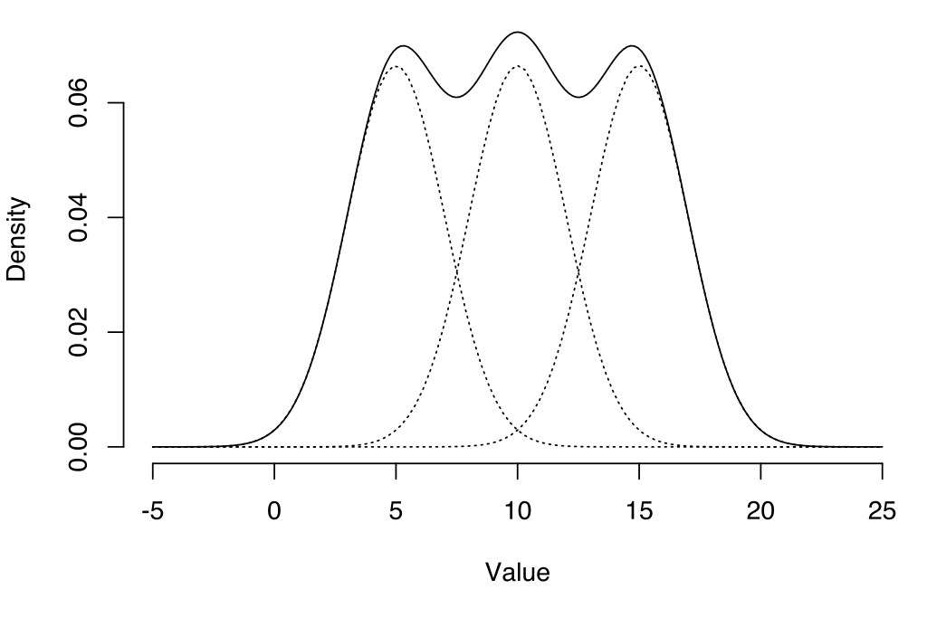
Figure 1. Density of a mixture of three normal distributions (μ 1 = 5 subscript 𝜇 1 5 \mu_{1}=5 μ 2 = 10 subscript 𝜇 2 10 \mu_{2}=10 μ 3 = 15 subscript 𝜇 3 15 \mu_{3}=15 σ 1 = σ 2 = σ 3 = 2 subscript 𝜎 1 subscript 𝜎 2 subscript 𝜎 3 2 \sigma_{1}=\sigma_{2}=\sigma_{3}=2
One of the central results about the spectrum of K P g subscript 𝐾 superscript 𝑃 𝑔 K_{P^{g}} [12 ] .
Theorem 1.9 ([12 ] , Theorem 3).
Let P = π 1 P 1 + π 2 P 2 𝑃 subscript 𝜋 1 superscript 𝑃 1 subscript 𝜋 2 superscript 𝑃 2 P=\pi_{1}P^{1}+\pi_{2}P^{2} ℝ l superscript ℝ 𝑙 \mathbb{R}^{l} π 1 + π 2 = 1 subscript 𝜋 1 subscript 𝜋 2 1 \pi_{1}+\pi_{2}=1 K 𝐾 K K P subscript 𝐾 𝑃 K_{P} K p 1 subscript 𝐾 superscript 𝑝 1 K_{p^{1}} K p 2 subscript 𝐾 superscript 𝑝 2 K_{p^{2}} λ 0 subscript 𝜆 0 \lambda_{0} λ 0 1 superscript subscript 𝜆 0 1 \lambda_{0}^{1} λ 0 2 superscript subscript 𝜆 0 2 \lambda_{0}^{2}
Then λ 0 subscript 𝜆 0 \lambda_{0} K P subscript 𝐾 𝑃 K_{P}
max ( π 1 λ 0 1 , π 2 λ 0 2 ) ≤ λ 0 ≤ max ( π 1 λ 0 1 , π 2 λ 0 2 ) + r subscript 𝜋 1 superscript subscript 𝜆 0 1 subscript 𝜋 2 superscript subscript 𝜆 0 2 subscript 𝜆 0 subscript 𝜋 1 superscript subscript 𝜆 0 1 subscript 𝜋 2 superscript subscript 𝜆 0 2 𝑟 \max(\pi_{1}\lambda_{0}^{1},\pi_{2}\lambda_{0}^{2})\leq\lambda_{0}\leq\max(\pi_{1}\lambda_{0}^{1},\pi_{2}\lambda_{0}^{2})+r
where
r = ( π 1 π 2 ∫ ∫ K ( x , z ) 2 𝑑 P 1 ( x ) 𝑑 P 2 ( z ) ) 1 / 2 . 𝑟 superscript subscript 𝜋 1 subscript 𝜋 2 𝐾 superscript 𝑥 𝑧 2 differential-d superscript 𝑃 1 𝑥 differential-d superscript 𝑃 2 𝑧 1 2 r=\left(\pi_{1}\pi_{2}\int\int K(x,z)^{2}dP^{1}(x)dP^{2}(z)\right)^{1/2}.
The same authors also provide an estimate on the leading eigenvector of the mixture distribution.
Corollary 1.10 ([12 ] , Corollary 2).
Let P = π 1 P 1 + π 2 P 2 𝑃 subscript 𝜋 1 superscript 𝑃 1 subscript 𝜋 2 superscript 𝑃 2 P=\pi_{1}P^{1}+\pi_{2}P^{2} ℝ l superscript ℝ 𝑙 \mathbb{R}^{l} π 1 + π 2 = 1 subscript 𝜋 1 subscript 𝜋 2 1 \pi_{1}+\pi_{2}=1 K 𝐾 K λ 0 subscript 𝜆 0 \lambda_{0} λ 0 1 superscript subscript 𝜆 0 1 \lambda_{0}^{1} λ 0 2 superscript subscript 𝜆 0 2 \lambda_{0}^{2} ϕ 0 subscript italic-ϕ 0 \phi_{0} ϕ 0 1 superscript subscript italic-ϕ 0 1 \phi_{0}^{1} ϕ 0 2 superscript subscript italic-ϕ 0 2 \phi_{0}^{2} K p subscript 𝐾 𝑝 K_{p} K p 1 subscript 𝐾 superscript 𝑝 1 K_{p^{1}} K p 2 subscript 𝐾 superscript 𝑝 2 K_{p^{2}} t = λ 0 − λ 1 𝑡 subscript 𝜆 0 subscript 𝜆 1 t=\lambda_{0}-\lambda_{1} K P subscript 𝐾 𝑃 K_{P} r 𝑟 r r < t 𝑟 𝑡 r<t
‖ π 2 ∫ ℝ d K ( x , y ) ϕ 0 1 ( y ) 𝑑 P 2 ( y ) ‖ L P 2 ≤ ϵ subscript norm subscript 𝜋 2 subscript superscript ℝ 𝑑 𝐾 𝑥 𝑦 superscript subscript italic-ϕ 0 1 𝑦 differential-d superscript 𝑃 2 𝑦 superscript subscript 𝐿 𝑃 2 italic-ϵ \left\|\pi_{2}\int_{\mathbb{R}^{d}}K(x,y)\phi_{0}^{1}(y)dP^{2}(y)\right\|_{L_{P}^{2}}\leq\epsilon
such that ϵ + r < t italic-ϵ 𝑟 𝑡 \epsilon+r<t π 1 λ 0 1 subscript 𝜋 1 superscript subscript 𝜆 0 1 \pi_{1}\lambda_{0}^{1} K P subscript 𝐾 𝑃 K_{P} λ 0 subscript 𝜆 0 \lambda_{0}
| π 1 λ 0 1 − λ 0 | ≤ ϵ subscript 𝜋 1 superscript subscript 𝜆 0 1 subscript 𝜆 0 italic-ϵ |\pi_{1}\lambda_{0}^{1}-\lambda_{0}|\leq\epsilon
and ϕ 0 1 superscript subscript italic-ϕ 0 1 \phi_{0}^{1} K P subscript 𝐾 𝑃 K_{P} ϕ 0 subscript italic-ϕ 0 \phi_{0} L P 2 superscript subscript 𝐿 𝑃 2 L_{P}^{2}
‖ ϕ 0 1 − ϕ 0 ‖ L P 2 ≤ ϵ t − ϵ . subscript norm superscript subscript italic-ϕ 0 1 subscript italic-ϕ 0 superscript subscript 𝐿 𝑃 2 italic-ϵ 𝑡 italic-ϵ \|\phi_{0}^{1}-\phi_{0}\|_{L_{P}^{2}}\leq\frac{\epsilon}{t-\epsilon}.
1.6. Gaussian components
The eigenvalues and the eigenvectors of the kernel operators for the univariate Gaussian N ( μ , σ 2 ) 𝑁 𝜇 superscript 𝜎 2 N(\mu,\sigma^{2}) [14 ] and [13 ] . Specifically, if one considers the kernel
K ( x , y ) = e − ( x − y ) 2 2 ω 2 , ω ∈ ℝ + , formulae-sequence 𝐾 𝑥 𝑦 superscript 𝑒 superscript 𝑥 𝑦 2 2 superscript 𝜔 2 𝜔 subscript ℝ K(x,y)=e^{-\frac{(x-y)^{2}}{2\omega^{2}}},\quad\omega\in\mathbb{R}_{+},
and the corresponding integral operator
K P ω f ( x ) superscript subscript 𝐾 𝑃 𝜔 𝑓 𝑥 \displaystyle K_{P}^{\omega}f(x) = ∫ ℝ K ( x , z ) f ( z ) p ( z ) 𝑑 z absent subscript ℝ 𝐾 𝑥 𝑧 𝑓 𝑧 𝑝 𝑧 differential-d 𝑧 \displaystyle=\int_{\mathbb{R}}K(x,z)f(z)p(z)dz
= ∫ ℝ e − ( z − x ) 2 2 ω 2 f ( z ) p ( z ) 𝑑 z , absent subscript ℝ superscript 𝑒 superscript 𝑧 𝑥 2 2 superscript 𝜔 2 𝑓 𝑧 𝑝 𝑧 differential-d 𝑧 \displaystyle=\int_{\mathbb{R}}e^{-\frac{(z-x)^{2}}{2\omega^{2}}}f(z)p(z)dz,
then the following holds.
Theorem 1.11 ([13 ] , Proposition 1).
Let β = 2 σ 2 / ω 2 𝛽 2 superscript 𝜎 2 superscript 𝜔 2 \beta=2\sigma^{2}/\omega^{2} H i ( x ) subscript 𝐻 𝑖 𝑥 H_{i}(x) i 𝑖 i K P ω superscript subscript 𝐾 𝑃 𝜔 K_{P}^{\omega} i = 0 , 1 , … , n 𝑖 0 1 … 𝑛
i=0,1,\ldots,n
λ i = 2 ( 1 + β + 1 + 2 β ) 1 / 2 ( β 1 + β + 1 + 2 β ) i , subscript 𝜆 𝑖 2 superscript 1 𝛽 1 2 𝛽 1 2 superscript 𝛽 1 𝛽 1 2 𝛽 𝑖 \displaystyle\lambda_{i}=\frac{\sqrt{2}}{(1+\beta+\sqrt{1+2\beta})^{1/2}}\left(\frac{\beta}{1+\beta+\sqrt{1+2\beta}}\right)^{i},
ϕ i ( x ) = ( 1 + 2 β ) 1 / 8 2 i i ! e − ( x − μ ) 2 2 σ 2 1 + 2 β − 1 2 H i [ ( 1 + 2 β 4 ) 1 / 4 x − μ σ ] . subscript italic-ϕ 𝑖 𝑥 superscript 1 2 𝛽 1 8 superscript 2 𝑖 𝑖 superscript 𝑒 superscript 𝑥 𝜇 2 2 superscript 𝜎 2 1 2 𝛽 1 2 subscript 𝐻 𝑖 delimited-[] superscript 1 2 𝛽 4 1 4 𝑥 𝜇 𝜎 \displaystyle\phi_{i}(x)=\frac{(1+2\beta)^{1/8}}{\sqrt{2^{i}i!}}e^{-\frac{(x-\mu)^{2}}{2\sigma^{2}}\frac{\sqrt{1+2\beta}-1}{2}}H_{i}\left[\left(\frac{1+2\beta}{4}\right)^{1/4}\frac{x-\mu}{\sigma}\right].
The eigenvalues form a geometric series with a common ratio
β 1 + β + 1 + 2 β < 1 . 𝛽 1 𝛽 1 2 𝛽 1 {\beta\over 1+\beta+\sqrt{1+2\beta}}<1.
It is clear that the sequence of the eigenvalues converges to zero faster for smaller values of β 𝛽 \beta
1.7. Multivariate Gaussian distribution
Theorem 1.12 ([13 ] ).
Let N ( μ , Σ ) 𝑁 𝜇 Σ N(\mu,\Sigma) ℝ d superscript ℝ 𝑑 \mathbb{R}^{d} Σ = Σ i = 1 d σ i 2 u i u i t Σ superscript subscript Σ 𝑖 1 𝑑 superscript subscript 𝜎 𝑖 2 subscript 𝑢 𝑖 superscript subscript 𝑢 𝑖 𝑡 \Sigma=\Sigma_{i=1}^{d}\sigma_{i}^{2}u_{i}u_{i}^{t} Σ Σ \Sigma
K P ω f ( x ) = ∫ ℝ d e − ‖ x − z ‖ 2 2 ω 2 f ( z ) p ( z ) 𝑑 z . superscript subscript 𝐾 𝑃 𝜔 𝑓 𝑥 subscript superscript ℝ 𝑑 superscript 𝑒 superscript norm 𝑥 𝑧 2 2 superscript 𝜔 2 𝑓 𝑧 𝑝 𝑧 differential-d 𝑧 K_{P}^{\omega}f(x)=\int_{\mathbb{R}^{d}}e^{-{\|x-z\|^{2}\over 2\omega^{2}}}f(z)p(z)dz.
Then K P ω superscript subscript 𝐾 𝑃 𝜔 K_{P}^{\omega}
K P ω = ⊕ i = 1 d K P i ω superscript subscript 𝐾 𝑃 𝜔 superscript subscript direct-sum 𝑖 1 𝑑 superscript subscript 𝐾 superscript 𝑃 𝑖 𝜔 K_{P}^{\omega}=\oplus_{i=1}^{d}K_{P^{i}}^{\omega}
where P i subscript 𝑃 𝑖 P_{i} σ i 2 superscript subscript 𝜎 𝑖 2 \sigma_{i}^{2} ⟨ μ , u i ⟩ 𝜇 subscript 𝑢 𝑖
\langle\mu,u_{i}\rangle u i subscript 𝑢 𝑖 u_{i}
Then the eigenvalues and eigenfunctions of K P ω superscript subscript 𝐾 𝑃 𝜔 K_{P}^{\omega}
λ [ i 1 , … , i d ] subscript 𝜆 subscript 𝑖 1 … subscript 𝑖 𝑑
\displaystyle\lambda_{[i_{1},\ldots,i_{d}]} = ∏ j = 1 d λ i j ( K p j ω ) , absent superscript subscript product 𝑗 1 𝑑 subscript 𝜆 subscript 𝑖 𝑗 superscript subscript 𝐾 subscript 𝑝 𝑗 𝜔 \displaystyle=\prod_{j=1}^{d}\lambda_{i_{j}}(K_{p_{j}}^{\omega}),
ϕ [ i 1 , … , i d ] ( K P ω ) ( x ) subscript italic-ϕ subscript 𝑖 1 … subscript 𝑖 𝑑
superscript subscript 𝐾 𝑃 𝜔 𝑥 \displaystyle\phi_{[i_{1},\ldots,i_{d}]}(K_{P}^{\omega})(x) = ∏ j = 1 d ( K p j ω ) ( ⟨ x , u j ⟩ ) absent superscript subscript product 𝑗 1 𝑑 superscript subscript 𝐾 subscript 𝑝 𝑗 𝜔 𝑥 subscript 𝑢 𝑗
\displaystyle=\prod_{j=1}^{d}(K_{p_{j}}^{\omega})(\langle x,u_{j}\rangle)
where [ i i , … , i d ] subscript 𝑖 𝑖 … subscript 𝑖 𝑑
[i_{i},\ldots,i_{d}]
2. Estimates on the second eigenvalue of a Gaussian mixture
In this Section we will provide bounds on the second eigenvalue of the kernel operator for a Gaussian mixture P = π 1 P 1 + π 2 P 2 𝑃 subscript 𝜋 1 superscript 𝑃 1 subscript 𝜋 2 superscript 𝑃 2 P=\pi_{1}P^{1}+\pi_{2}P^{2} 1.9
Main theorem: Second leading eigenvalue of mixture distribution .
Let P = π 1 + P 1 + π 2 P 2 𝑃 subscript 𝜋 1 superscript 𝑃 1 subscript 𝜋 2 superscript 𝑃 2 P=\pi_{1}+P^{1}+\pi_{2}P^{2} K P subscript 𝐾 𝑃 K_{P} K P 1 subscript 𝐾 subscript 𝑃 1 K_{P_{1}} K P 2 subscript 𝐾 subscript 𝑃 2 K_{P_{2}} λ 0 subscript 𝜆 0 \lambda_{0} λ 1 subscript 𝜆 1 \lambda_{1} γ 0 subscript 𝛾 0 \gamma_{0} γ 1 subscript 𝛾 1 \gamma_{1} ν 0 subscript 𝜈 0 \nu_{0} ν 1 subscript 𝜈 1 \nu_{1} ∥ ⋅ ∥ P = ∥ ⋅ ∥ L P 2 \|\cdot\|_{P}=\|\cdot\|_{L^{2}_{P}} P 1 superscript 𝑃 1 P^{1} P 2 superscript 𝑃 2 P^{2} π 1 > π 2 subscript 𝜋 1 subscript 𝜋 2 \pi_{1}>\pi_{2}
δ ( z ) = ϕ 0 1 ( z ) − ϕ 0 ( z ) . 𝛿 𝑧 superscript subscript italic-ϕ 0 1 𝑧 subscript italic-ϕ 0 𝑧 \delta(z)=\phi_{0}^{1}(z)-\phi_{0}(z).
Then an upper bound for λ 1 subscript 𝜆 1 \lambda_{1}
λ 1 ≤ π 1 2 γ 1 ( 1 π 1 + 2 π 1 A + A ) subscript 𝜆 1 superscript subscript 𝜋 1 2 subscript 𝛾 1 1 subscript 𝜋 1 2 subscript 𝜋 1 𝐴 𝐴 \displaystyle\lambda_{1}\leq\pi_{1}^{2}\gamma_{1}\left(\frac{1}{\pi_{1}}+\frac{2}{\sqrt{\pi_{1}}}A+A\right) + 2 π 1 2 ‖ K ‖ P 1 × P 1 ( 1 π 1 + A ) A 2 superscript subscript 𝜋 1 2 subscript norm 𝐾 superscript 𝑃 1 superscript 𝑃 1 1 subscript 𝜋 1 𝐴 𝐴 \displaystyle+2\pi_{1}^{2}\left\|K\right\|_{{P^{1}}\times{P^{1}}}\left(\frac{1}{\sqrt{\pi_{1}}}+A\right)A
+ π 1 2 ‖ K ‖ P 1 × P 1 A 2 + r superscript subscript 𝜋 1 2 subscript norm 𝐾 superscript 𝑃 1 superscript 𝑃 1 superscript 𝐴 2 𝑟 \displaystyle+\pi_{1}^{2}\left\|K\right\|_{{P^{1}}\times{P^{1}}}A^{2}+r
where
A ≤ ‖ δ ‖ P 2 + 2 ‖ δ ‖ P Δ + Δ 2 , Δ 𝐴 subscript superscript norm 𝛿 2 𝑃 2 subscript norm 𝛿 𝑃 Δ superscript Δ 2 Δ
\displaystyle A\leq\|\delta\|^{2}_{P}+2\|\delta\|_{P}\Delta+\Delta^{2},\quad\Delta ≤ ( 1 π 1 − 1 ) ‖ ϕ 0 1 ‖ P + 1 π 1 ‖ ϕ 0 1 ‖ P 2 absent 1 subscript 𝜋 1 1 subscript norm superscript subscript italic-ϕ 0 1 𝑃 1 subscript 𝜋 1 subscript norm superscript subscript italic-ϕ 0 1 superscript 𝑃 2 \displaystyle\leq\left(\frac{1}{\pi_{1}}-1\right)\|\phi_{0}^{1}\|_{P}+\frac{1}{\pi_{1}}\|\phi_{0}^{1}\|_{P^{2}}
and
r = ( π 1 π 2 ∬ K ( x , z ) 2 𝑑 P 1 ( x ) 𝑑 P 2 ( z ) ) 1 2 . 𝑟 superscript subscript 𝜋 1 subscript 𝜋 2 double-integral 𝐾 superscript 𝑥 𝑧 2 differential-d superscript 𝑃 1 𝑥 differential-d superscript 𝑃 2 𝑧 1 2 r=\left(\pi_{1}\pi_{2}\iint K(x,z)^{2}dP^{1}(x)dP^{2}(z)\right)^{1\over 2}.
Moreover, a lower bound is given by
λ 1 ≥ 1 D 1 + D 2 [ π 1 2 γ 1 + π 1 π 2 ∥ ϕ 1 1 ∥ P 2 2 − π 2 ∥ ϕ 1 1 ∥ P ∥ ϕ 1 1 ∥ P 2 ∥ K ∥ P 2 × P − − 2 | e | | λ 0 ⋅ ∥ δ ∥ P ⋅ ∥ ϕ 1 1 ∥ P + λ 0 ∫ ϕ 1 1 ( x ) ϕ 0 1 ( x ) d P ( x ) | − e 2 λ 0 ] \begin{split}\lambda_{1}&\geq\frac{1}{D_{1}+D_{2}}\left[\phantom{\int}\pi_{1}^{2}\gamma_{1}+\pi_{1}\pi_{2}\|\phi_{1}^{1}\|^{2}_{P^{2}}-\pi_{2}\|\phi_{1}^{1}\|_{P}\|\phi_{1}^{1}\|_{P^{2}}\|K\|_{P^{2}\times P}-\right.\\
&\hskip 30.0pt\left.-2|e|\left|\lambda_{0}\cdot\|\delta\|_{P}\cdot\|\phi_{1}^{1}\|_{P}+\lambda_{0}\int\phi_{1}^{1}(x)\phi_{0}^{1}(x)dP(x)\right|-e^{2}\lambda_{0}\right]\end{split}
where
D 1 subscript 𝐷 1 \displaystyle D_{1} = π 1 + 2 | e | π 1 ‖ δ ‖ P + e 2 + 2 e 2 π 1 ‖ δ ‖ P + e 2 π 1 ‖ δ ‖ P 2 , absent subscript 𝜋 1 2 𝑒 subscript 𝜋 1 subscript norm 𝛿 𝑃 superscript 𝑒 2 2 superscript 𝑒 2 subscript 𝜋 1 subscript norm 𝛿 𝑃 superscript 𝑒 2 subscript 𝜋 1 subscript superscript norm 𝛿 2 𝑃 \displaystyle=\pi_{1}+2|e|\pi_{1}\|\delta\|_{P}+e^{2}+2e^{2}\pi_{1}\|\delta\|_{P}+e^{2}\pi_{1}\|\delta\|^{2}_{P},
D 2 subscript 𝐷 2 \displaystyle D_{2} = π 2 ‖ ϕ 1 1 ‖ P 2 2 + 2 | e | π 2 ‖ δ ‖ P ‖ ϕ 1 1 ‖ P 2 + e 2 π 2 ‖ ϕ 0 1 ‖ 2 + absent subscript 𝜋 2 subscript superscript norm superscript subscript italic-ϕ 1 1 2 superscript 𝑃 2 2 𝑒 subscript 𝜋 2 subscript norm 𝛿 𝑃 subscript norm superscript subscript italic-ϕ 1 1 superscript 𝑃 2 limit-from superscript 𝑒 2 subscript 𝜋 2 superscript norm superscript subscript italic-ϕ 0 1 2 \displaystyle=\pi_{2}\|\phi_{1}^{1}\|^{2}_{P^{2}}+2|e|\pi_{2}\|\delta\|_{P}\|\phi_{1}^{1}\|_{P^{2}}+e^{2}\pi_{2}\|\phi_{0}^{1}\|^{2}+
+ 2 e 2 π 2 ‖ δ ‖ P ‖ ϕ 0 1 ‖ P 2 + e 2 π 2 ‖ δ ‖ P 2 2 superscript 𝑒 2 subscript 𝜋 2 subscript norm 𝛿 𝑃 subscript norm superscript subscript italic-ϕ 0 1 superscript 𝑃 2 superscript 𝑒 2 subscript 𝜋 2 subscript superscript norm 𝛿 2 𝑃 \displaystyle\phantom{=\pi_{2}\|\phi_{1}^{1}\|^{2}_{P^{2}}}+2e^{2}\pi_{2}\|\delta\|_{P}\|\phi_{0}^{1}\|_{P^{2}}+e^{2}\pi_{2}\|\delta\|^{2}_{P}
and where
e = ∫ ϕ 1 1 ( ϕ 0 1 − ϕ 0 ) 𝑑 P − π 2 ∫ ϕ 1 1 ϕ 0 1 𝑑 P 2 . 𝑒 superscript subscript italic-ϕ 1 1 superscript subscript italic-ϕ 0 1 subscript italic-ϕ 0 differential-d 𝑃 subscript 𝜋 2 superscript subscript italic-ϕ 1 1 superscript subscript italic-ϕ 0 1 differential-d superscript 𝑃 2 e=\int\phi_{1}^{1}(\phi_{0}^{1}-\phi_{0})dP-\pi_{2}\int\phi_{1}^{1}\phi_{0}^{1}dP^{2}.
Proof.
Upper bound. We first prove the upper bound. For this, we present the standard calculation for f 𝑓 f V 𝑉 V ϕ 0 subscript italic-ϕ 0 \phi_{0} L P 2 subscript superscript 𝐿 2 𝑃 L^{2}_{P}
(4) λ 1 = max f ∈ V ∬ K ( x , z ) f ( x ) f ( z ) 𝑑 P ( x ) 𝑑 P ( z ) ∫ f ( x ) 2 𝑑 P ( x ) , subscript 𝜆 1 subscript 𝑓 𝑉 double-integral 𝐾 𝑥 𝑧 𝑓 𝑥 𝑓 𝑧 differential-d 𝑃 𝑥 differential-d 𝑃 𝑧 𝑓 superscript 𝑥 2 differential-d 𝑃 𝑥 \lambda_{1}=\max_{f\in V}\frac{\iint K(x,z)f(x)f(z)dP(x)dP(z)}{\int f(x)^{2}dP(x)},
and that for any such f 𝑓 f
∬ double-integral \displaystyle\iint K ( x , z ) f ( x ) f ( z ) d P ( x ) d P ( z ) = π 1 2 ∬ K ( x , z ) f ( x ) f ( z ) 𝑑 P 1 ( x ) 𝑑 P 1 ( z ) 𝐾 𝑥 𝑧 𝑓 𝑥 𝑓 𝑧 𝑑 𝑃 𝑥 𝑑 𝑃 𝑧 superscript subscript 𝜋 1 2 double-integral 𝐾 𝑥 𝑧 𝑓 𝑥 𝑓 𝑧 differential-d superscript 𝑃 1 𝑥 differential-d superscript 𝑃 1 𝑧 \displaystyle K(x,z)f(x)f(z)dP(x)dP(z)=\pi_{1}^{2}\iint K(x,z)f(x)f(z)dP^{1}(x)dP^{1}(z)
+ π 2 2 ∬ K ( x , z ) f ( x ) f ( z ) 𝑑 P 2 ( x ) 𝑑 P 2 ( z ) + limit-from superscript subscript 𝜋 2 2 double-integral 𝐾 𝑥 𝑧 𝑓 𝑥 𝑓 𝑧 differential-d superscript 𝑃 2 𝑥 differential-d superscript 𝑃 2 𝑧 \displaystyle\hskip 20.0pt+\pi_{2}^{2}\iint K(x,z)f(x)f(z)dP^{2}(x)dP^{2}(z)+
+ 2 π 1 π 2 ∬ K ( x , z ) f ( x ) f ( z ) 𝑑 P 1 ( x ) 𝑑 P 2 ( z ) 2 subscript 𝜋 1 subscript 𝜋 2 double-integral 𝐾 𝑥 𝑧 𝑓 𝑥 𝑓 𝑧 differential-d superscript 𝑃 1 𝑥 differential-d superscript 𝑃 2 𝑧 \displaystyle\hskip 20.0pt+2\pi_{1}\pi_{2}\iint K(x,z)f(x)f(z)dP^{1}(x)dP^{2}(z)
≤ π 1 2 ∬ K ( x , z ) ( f ( z ) − ( proj ϕ 0 1 1 f ) ϕ 0 1 ( z ) + F ( z ) ) × \displaystyle\leq\pi_{1}^{2}\iint K(x,z)\left(f(z)-(\textrm{proj}^{1}_{\phi_{0}^{1}}f)\phi_{0}^{1}(z)+F(z)\right)\times
× ( f ( x ) − ( proj ϕ 0 1 1 f ) ϕ 0 1 ( x ) + F ( x ) ) d P 1 ( z ) d P 1 ( x ) + absent limit-from 𝑓 𝑥 subscript superscript proj 1 superscript subscript italic-ϕ 0 1 𝑓 superscript subscript italic-ϕ 0 1 𝑥 𝐹 𝑥 𝑑 superscript 𝑃 1 𝑧 𝑑 superscript 𝑃 1 𝑥 \displaystyle\hskip 20.0pt\times\left(f(x)-(\textrm{proj}^{1}_{\phi_{0}^{1}}f)\phi_{0}^{1}(x)+F(x)\right)dP^{1}(z)dP^{1}(x)+
+ π 2 2 ν 0 ∫ ( f ( x ) ) 2 𝑑 P 2 ( x ) + limit-from superscript subscript 𝜋 2 2 subscript 𝜈 0 superscript 𝑓 𝑥 2 differential-d superscript 𝑃 2 𝑥 \displaystyle\hskip 20.0pt+\pi_{2}^{2}\nu_{0}\int(f(x))^{2}dP^{2}(x)+
(5) + 2 π 1 π 2 ∬ K ( x , z ) f ( x ) f ( z ) 𝑑 P 1 ( x ) 𝑑 P 2 ( z ) , 2 subscript 𝜋 1 subscript 𝜋 2 double-integral 𝐾 𝑥 𝑧 𝑓 𝑥 𝑓 𝑧 differential-d superscript 𝑃 1 𝑥 differential-d superscript 𝑃 2 𝑧 \displaystyle\hskip 20.0pt+2\pi_{1}\pi_{2}\iint K(x,z)f(x)f(z)dP^{1}(x)dP^{2}(z),
where
proj ϕ i f = ∫ ϕ ( x ) f ( x ) 𝑑 P i ( x ) , proj ϕ f = ∫ ϕ ( x ) f ( x ) 𝑑 P ( x ) formulae-sequence subscript superscript proj 𝑖 italic-ϕ 𝑓 italic-ϕ 𝑥 𝑓 𝑥 differential-d superscript 𝑃 𝑖 𝑥 subscript proj italic-ϕ 𝑓 italic-ϕ 𝑥 𝑓 𝑥 differential-d 𝑃 𝑥 \textrm{proj}^{i}_{\phi}f=\int\phi(x)f(x)dP^{i}(x),\quad\textrm{proj}_{\phi}f=\int\phi(x)f(x)dP(x)
and
F ( z ) = ( proj ϕ 0 1 1 f ) ϕ 0 1 ( z ) = ( proj ϕ 0 1 1 f − proj ϕ 0 f ) ϕ 0 1 ( z ) 𝐹 𝑧 subscript superscript proj 1 superscript subscript italic-ϕ 0 1 𝑓 superscript subscript italic-ϕ 0 1 𝑧 subscript superscript proj 1 superscript subscript italic-ϕ 0 1 𝑓 subscript proj subscript italic-ϕ 0 𝑓 superscript subscript italic-ϕ 0 1 𝑧 F(z)=(\textrm{proj}^{1}_{\phi_{0}^{1}}f)\phi_{0}^{1}(z)=(\textrm{proj}^{1}_{\phi_{0}^{1}}f-\textrm{proj}_{\phi_{0}}f)\phi_{0}^{1}(z)
and where the second equality follows from f ∈ V 𝑓 𝑉 f\in V ( 5 ) 5 (\ref{upper1})
(6) ∬ double-integral \displaystyle\iint K ( x , z ) f ( x ) f ( z ) d P ( x ) d P ( z ) 𝐾 𝑥 𝑧 𝑓 𝑥 𝑓 𝑧 𝑑 𝑃 𝑥 𝑑 𝑃 𝑧 \displaystyle K(x,z)f(x)f(z)dP(x)dP(z)
≤ π 1 2 γ 1 ∫ ( f ( x ) − ( proj ϕ 0 1 1 f ) ϕ 0 1 ( x ) ) 2 𝑑 P 1 ( x ) + absent limit-from superscript subscript 𝜋 1 2 subscript 𝛾 1 superscript 𝑓 𝑥 subscript superscript proj 1 superscript subscript italic-ϕ 0 1 𝑓 superscript subscript italic-ϕ 0 1 𝑥 2 differential-d superscript 𝑃 1 𝑥 \displaystyle\leq\pi_{1}^{2}\gamma_{1}\int\left(f(x)-(\textrm{proj}^{1}_{\phi_{0}^{1}}f)\phi_{0}^{1}(x)\right)^{2}dP^{1}(x)+
+ 2 π 1 2 ∬ K ( x , z ) ( f ( z ) − ( proj ϕ 0 1 1 f ) ϕ 0 1 ( z ) ) F ( x ) 𝑑 P 1 ( z ) 𝑑 P 1 ( x ) + limit-from 2 superscript subscript 𝜋 1 2 double-integral 𝐾 𝑥 𝑧 𝑓 𝑧 subscript superscript proj 1 superscript subscript italic-ϕ 0 1 𝑓 superscript subscript italic-ϕ 0 1 𝑧 𝐹 𝑥 differential-d superscript 𝑃 1 𝑧 differential-d superscript 𝑃 1 𝑥 \displaystyle\hskip 10.0pt+2\pi_{1}^{2}\iint K(x,z)\left(f(z)-(\textrm{proj}^{1}_{\phi_{0}^{1}}f)\phi_{0}^{1}(z)\right)F(x)\ dP^{1}(z)dP^{1}(x)+
+ π 1 2 ∬ K ( x , z ) F ( z ) F ( x ) 𝑑 P 1 ( z ) 𝑑 P 1 ( x ) + limit-from superscript subscript 𝜋 1 2 double-integral 𝐾 𝑥 𝑧 𝐹 𝑧 𝐹 𝑥 differential-d superscript 𝑃 1 𝑧 differential-d superscript 𝑃 1 𝑥 \displaystyle\hskip 10.0pt+\pi_{1}^{2}\iint K(x,z)F(z)F(x)\ dP^{1}(z)dP^{1}(x)+
+ π 2 2 ν 0 ∫ f ( x ) 2 𝑑 P 2 ( x ) + limit-from superscript subscript 𝜋 2 2 subscript 𝜈 0 𝑓 superscript 𝑥 2 differential-d superscript 𝑃 2 𝑥 \displaystyle\hskip 10.0pt+\pi_{2}^{2}\nu_{0}\int f(x)^{2}dP^{2}(x)+
+ 2 π 1 π 2 ∬ K ( x , z ) f ( x ) f ( z ) 𝑑 P 1 ( x ) 𝑑 P 2 ( z ) . 2 subscript 𝜋 1 subscript 𝜋 2 double-integral 𝐾 𝑥 𝑧 𝑓 𝑥 𝑓 𝑧 differential-d superscript 𝑃 1 𝑥 differential-d superscript 𝑃 2 𝑧 \displaystyle\hskip 10.0pt+2\pi_{1}\pi_{2}\iint K(x,z)f(x)f(z)dP^{1}(x)dP^{2}(z).
We take the terms one by one in (6
∫ ( f ( x ) − ( proj ϕ 0 1 1 f ) ϕ 0 1 ( x ) ) 2 𝑑 P 1 ( x ) superscript 𝑓 𝑥 subscript superscript proj 1 superscript subscript italic-ϕ 0 1 𝑓 superscript subscript italic-ϕ 0 1 𝑥 2 differential-d superscript 𝑃 1 𝑥 \displaystyle\int\left(f(x)-(\textrm{proj}^{1}_{\phi_{0}^{1}}f)\phi_{0}^{1}(x)\right)^{2}dP^{1}(x) = ‖ f − ( proj ϕ 0 1 1 ) ϕ 0 1 ‖ 2 absent superscript norm 𝑓 subscript superscript proj 1 superscript subscript italic-ϕ 0 1 superscript subscript italic-ϕ 0 1 2 \displaystyle=\|f-(\textrm{proj}^{1}_{\phi_{0}^{1}})\phi_{0}^{1}\|^{2}
≤ ( ‖ f ‖ P 1 + ‖ F ‖ P 1 ) 2 absent superscript subscript norm 𝑓 superscript 𝑃 1 subscript norm 𝐹 superscript 𝑃 1 2 \displaystyle\leq\left(\|f\|_{P^{1}}+\|F\|_{P^{1}}\right)^{2}
≤ ( 1 π 1 + ‖ F ‖ P 1 ) 2 absent superscript 1 subscript 𝜋 1 subscript norm 𝐹 superscript 𝑃 1 2 \displaystyle\leq\left(\frac{1}{\sqrt{\pi_{1}}}+\|F\|_{P^{1}}\right)^{2}
where we in the last step have normalized f 𝑓 f
For the second term, we write
| ∬ K ( x , z ) ( f ( z ) − ( proj ϕ 0 1 f ) ϕ 0 1 ( z ) ) F ( x ) 𝑑 P 1 ( z ) 𝑑 P 1 ( x ) | double-integral 𝐾 𝑥 𝑧 𝑓 𝑧 subscript proj superscript subscript italic-ϕ 0 1 𝑓 superscript subscript italic-ϕ 0 1 𝑧 𝐹 𝑥 differential-d superscript 𝑃 1 𝑧 differential-d superscript 𝑃 1 𝑥 \displaystyle\left|\iint K(x,z)\left(f(z)-(\textrm{proj}_{\phi_{0}^{1}}f)\phi_{0}^{1}(z)\right)F(x)dP^{1}(z)dP^{1}(x)\right|
= | ∫ ( ∫ K ( x , z ) ( f ( z ) − ( proj ϕ 0 1 f ) ϕ 0 1 ( z ) ) 𝑑 P 1 ( z ) ) F ( x ) 𝑑 P 1 ( x ) | absent 𝐾 𝑥 𝑧 𝑓 𝑧 subscript proj superscript subscript italic-ϕ 0 1 𝑓 superscript subscript italic-ϕ 0 1 𝑧 differential-d superscript 𝑃 1 𝑧 𝐹 𝑥 differential-d superscript 𝑃 1 𝑥 \displaystyle\hskip 20.0pt=\left|\int\left(\int K(x,z)\left(f(z)-(\textrm{proj}_{\phi_{0}^{1}}f)\phi_{0}^{1}(z)\right)dP^{1}(z)\right)F(x)dP^{1}(x)\right|
≤ ∫ ( ∫ K ( x , z ) ( f ( z ) − ( proj ϕ 0 1 f ) ϕ 0 1 ( z ) ) 𝑑 P 1 ( z ) ) 2 𝑑 P 1 ( x ) ‖ F ‖ P 1 absent superscript 𝐾 𝑥 𝑧 𝑓 𝑧 subscript proj superscript subscript italic-ϕ 0 1 𝑓 superscript subscript italic-ϕ 0 1 𝑧 differential-d superscript 𝑃 1 𝑧 2 differential-d superscript 𝑃 1 𝑥 subscript norm 𝐹 superscript 𝑃 1 \displaystyle\hskip 20.0pt\leq\sqrt{\int\left(\int K(x,z)\left(f(z)-(\textrm{proj}_{\phi_{0}^{1}}f)\phi_{0}^{1}(z)\right)dP^{1}(z)\right)^{2}dP^{1}(x)}\left\|F\right\|_{{P^{1}}}
≤ ∫ ∫ K ( x , z ) 2 𝑑 P 1 ( z ) ‖ f − ( proj ϕ 0 1 f ) ϕ 0 1 ‖ P 1 2 𝑑 P 1 ( x ) ‖ F ‖ P 1 absent 𝐾 superscript 𝑥 𝑧 2 differential-d superscript 𝑃 1 𝑧 subscript superscript norm 𝑓 subscript proj superscript subscript italic-ϕ 0 1 𝑓 superscript subscript italic-ϕ 0 1 2 superscript 𝑃 1 differential-d superscript 𝑃 1 𝑥 subscript norm 𝐹 superscript 𝑃 1 \displaystyle\hskip 20.0pt\leq\sqrt{\int\int K(x,z)^{2}dP^{1}(z)\left\|f-(\textrm{proj}_{\phi_{0}^{1}}f)\phi_{0}^{1}\right\|^{2}_{{P^{1}}}dP^{1}(x)}\left\|F\right\|_{{P^{1}}}
≤ ‖ K ‖ P 1 × P 1 ‖ f − ( proj ϕ 0 1 f ) ϕ 0 1 ‖ P 1 ‖ F ‖ P 1 absent subscript norm 𝐾 superscript 𝑃 1 superscript 𝑃 1 subscript norm 𝑓 subscript proj superscript subscript italic-ϕ 0 1 𝑓 superscript subscript italic-ϕ 0 1 superscript 𝑃 1 subscript norm 𝐹 superscript 𝑃 1 \displaystyle\hskip 20.0pt\leq\left\|K\right\|_{{P^{1}}\times{P^{1}}}\left\|f-(\textrm{proj}_{\phi_{0}^{1}}f)\phi_{0}^{1}\right\|_{{P^{1}}}\left\|F\right\|_{{P^{1}}}
≤ ‖ K ‖ P 1 × P 1 ( ‖ f ‖ P 1 + ‖ F ‖ P 1 ) ‖ F ‖ P 1 absent subscript norm 𝐾 superscript 𝑃 1 superscript 𝑃 1 subscript norm 𝑓 superscript 𝑃 1 subscript norm 𝐹 superscript 𝑃 1 subscript norm 𝐹 superscript 𝑃 1 \displaystyle\hskip 20.0pt\leq\left\|K\right\|_{{P^{1}}\times{P^{1}}}\left(\|f\|_{P^{1}}+\|F\|_{P^{1}}\right)\left\|F\right\|_{{P^{1}}}
≤ ‖ K ‖ P 1 × P 1 ( 1 π 1 + ‖ F ‖ P 1 ) ‖ F ‖ P 1 . absent subscript norm 𝐾 superscript 𝑃 1 superscript 𝑃 1 1 subscript 𝜋 1 subscript norm 𝐹 superscript 𝑃 1 subscript norm 𝐹 superscript 𝑃 1 \displaystyle\hskip 20.0pt\leq\left\|K\right\|_{{P^{1}}\times{P^{1}}}\left(\frac{1}{\sqrt{\pi_{1}}}+\|F\|_{P^{1}}\right)\left\|F\right\|_{{P^{1}}}.
For the third term,
| ∬ K ( x , z ) F ( z ) F ( x ) 𝑑 P 1 ( z ) 𝑑 P 1 ( x ) | ≤ ‖ K ‖ P 1 × P 1 ‖ F ‖ P 1 2 . double-integral 𝐾 𝑥 𝑧 𝐹 𝑧 𝐹 𝑥 differential-d superscript 𝑃 1 𝑧 differential-d superscript 𝑃 1 𝑥 subscript norm 𝐾 superscript 𝑃 1 superscript 𝑃 1 subscript superscript norm 𝐹 2 superscript 𝑃 1 \left|\iint K(x,z)F(z)F(x)dP^{1}(z)dP^{1}(x)\right|\leq\left\|K\right\|_{{P^{1}}\times{P^{1}}}\left\|F\right\|^{2}_{{P^{1}}}.
For the fourth,
π 2 2 ν 0 ∫ f ( x ) 2 𝑑 P 2 ( x ) ≤ π 2 ν 0 . superscript subscript 𝜋 2 2 subscript 𝜈 0 𝑓 superscript 𝑥 2 differential-d superscript 𝑃 2 𝑥 subscript 𝜋 2 subscript 𝜈 0 \displaystyle\pi_{2}^{2}\nu_{0}\int f(x)^{2}dP^{2}(x)\leq\pi_{2}\nu_{0}.
For the last term,
2 π 1 π 2 ∬ K ( x , z ) f ( x ) f ( z ) 𝑑 P 1 ( x ) 𝑑 P 2 ( z ) 2 subscript 𝜋 1 subscript 𝜋 2 double-integral 𝐾 𝑥 𝑧 𝑓 𝑥 𝑓 𝑧 differential-d superscript 𝑃 1 𝑥 differential-d superscript 𝑃 2 𝑧 \displaystyle 2\pi_{1}\pi_{2}\iint K(x,z)f(x)f(z)dP^{1}(x)dP^{2}(z)
≤ 2 π 1 π 2 ∬ K ( x , z ) 2 𝑑 P 1 ( x ) 𝑑 P 2 ( z ) ∬ f ( x ) 2 f ( z ) 2 𝑑 P 1 ( x ) 𝑑 P 2 ( z ) absent 2 subscript 𝜋 1 subscript 𝜋 2 double-integral 𝐾 superscript 𝑥 𝑧 2 differential-d superscript 𝑃 1 𝑥 differential-d superscript 𝑃 2 𝑧 double-integral 𝑓 superscript 𝑥 2 𝑓 superscript 𝑧 2 differential-d superscript 𝑃 1 𝑥 differential-d superscript 𝑃 2 𝑧 \displaystyle\hskip 5.0pt\leq 2\pi_{1}\pi_{2}\sqrt{\iint K(x,z)^{2}dP^{1}(x)dP^{2}(z)}\sqrt{\iint f(x)^{2}f(z)^{2}dP^{1}(x)dP^{2}(z)}
= 2 π 1 π 2 ∬ K ( x , z ) 2 𝑑 P 1 ( x ) 𝑑 P 2 ( z ) × \displaystyle\hskip 5.0pt=2\sqrt{\pi_{1}\pi_{2}\iint K(x,z)^{2}dP^{1}(x)dP^{2}(z)}\times
× π 1 ∫ f ( x ) 2 𝑑 P 1 ( x ) π 2 ∫ f ( z ) 2 𝑑 P 2 ( x ) absent subscript 𝜋 1 𝑓 superscript 𝑥 2 differential-d superscript 𝑃 1 𝑥 subscript 𝜋 2 𝑓 superscript 𝑧 2 differential-d superscript 𝑃 2 𝑥 \displaystyle\hskip 140.0pt\times\sqrt{\pi_{1}\int f(x)^{2}dP^{1}(x)}\sqrt{\pi_{2}\int f(z)^{2}dP^{2}(x)}
≤ π 1 π 2 ∬ K ( x , z ) 2 𝑑 P 1 ( x ) 𝑑 P 2 ( z ) × \displaystyle\hskip 5.0pt\leq\sqrt{\pi_{1}\pi_{2}\iint K(x,z)^{2}dP^{1}(x)dP^{2}(z)}\times
× ( π 1 ∫ f ( x ) 2 𝑑 P 1 ( x ) + π 2 ∫ f ( z ) 2 𝑑 P 2 ( x ) ) absent subscript 𝜋 1 𝑓 superscript 𝑥 2 differential-d superscript 𝑃 1 𝑥 subscript 𝜋 2 𝑓 superscript 𝑧 2 differential-d superscript 𝑃 2 𝑥 \displaystyle\hskip 140.0pt\times\left(\pi_{1}\int f(x)^{2}dP^{1}(x)+\pi_{2}\int f(z)^{2}dP^{2}(x)\right)
= r ∫ f ( x ) 2 𝑑 P ( x ) , absent 𝑟 𝑓 superscript 𝑥 2 differential-d 𝑃 𝑥 \displaystyle\hskip 5.0pt=r\int f(x)^{2}dP(x),
where
r = ( π 1 π 2 ∬ K ( x , z ) 2 𝑑 P 1 ( x ) 𝑑 P 2 ( z ) ) 1 2 . 𝑟 superscript subscript 𝜋 1 subscript 𝜋 2 double-integral 𝐾 superscript 𝑥 𝑧 2 differential-d superscript 𝑃 1 𝑥 differential-d superscript 𝑃 2 𝑧 1 2 r=\left(\pi_{1}\pi_{2}\iint K(x,z)^{2}dP^{1}(x)dP^{2}(z)\right)^{1\over 2}.
Finally,
λ 1 subscript 𝜆 1 \displaystyle\lambda_{1} ≤ π 1 2 γ 1 ( 1 π 1 + ‖ F ‖ P 1 ) 2 + 2 π 1 2 ( ‖ K ‖ P 1 × P 1 ( 1 π 1 + ‖ F ‖ P 1 ) ‖ F ‖ P 1 ) absent superscript subscript 𝜋 1 2 subscript 𝛾 1 superscript 1 subscript 𝜋 1 subscript norm 𝐹 superscript 𝑃 1 2 2 superscript subscript 𝜋 1 2 subscript norm 𝐾 superscript 𝑃 1 superscript 𝑃 1 1 subscript 𝜋 1 subscript norm 𝐹 superscript 𝑃 1 subscript norm 𝐹 superscript 𝑃 1 \displaystyle\leq\pi_{1}^{2}\gamma_{1}\left(\frac{1}{\sqrt{\pi_{1}}}+\|F\|_{P^{1}}\right)^{2}+2\pi_{1}^{2}\left(\left\|K\right\|_{{P^{1}}\times{P^{1}}}\left(\frac{1}{\sqrt{\pi_{1}}}+\|F\|_{P^{1}}\right)\left\|F\right\|_{{P^{1}}}\right)
+ π 1 2 ‖ K ‖ P 1 × P 1 ‖ F ‖ P 1 2 + r . superscript subscript 𝜋 1 2 subscript norm 𝐾 superscript 𝑃 1 superscript 𝑃 1 subscript superscript norm 𝐹 2 superscript 𝑃 1 𝑟 \displaystyle\phantom{\leq\pi_{1}^{2}\gamma_{1}\left(\frac{1}{\sqrt{\pi_{1}}}+\|F\|_{P^{1}}\right)^{2}\ }+\pi_{1}^{2}\left\|K\right\|_{{P^{1}}\times{P^{1}}}\left\|F\right\|^{2}_{{P^{1}}}+r.
Lower bound. Let
ϕ ~ 1 1 = ϕ 1 1 − ( proj ϕ 0 ϕ 1 1 ) ϕ 0 = ϕ 1 1 + ϕ 0 ( proj ϕ 0 1 1 ϕ 1 1 − proj ϕ 0 ϕ 1 1 ) , superscript subscript ~ italic-ϕ 1 1 superscript subscript italic-ϕ 1 1 subscript proj subscript italic-ϕ 0 superscript subscript italic-ϕ 1 1 subscript italic-ϕ 0 superscript subscript italic-ϕ 1 1 subscript italic-ϕ 0 subscript superscript proj 1 superscript subscript italic-ϕ 0 1 superscript subscript italic-ϕ 1 1 subscript proj subscript italic-ϕ 0 superscript subscript italic-ϕ 1 1 \widetilde{\phi}_{1}^{1}=\phi_{1}^{1}-(\textrm{proj}_{\phi_{0}}\phi_{1}^{1})\phi_{0}=\phi_{1}^{1}+\phi_{0}(\textrm{proj}^{1}_{\phi_{0}^{1}}\phi_{1}^{1}-\textrm{proj}_{\phi_{0}}\phi_{1}^{1}),
where in the second equality we have used that ( proj ϕ 0 1 1 ϕ 1 1 ) ϕ 0 = 0 subscript superscript proj 1 superscript subscript italic-ϕ 0 1 superscript subscript italic-ϕ 1 1 subscript italic-ϕ 0 0 (\textrm{proj}^{1}_{\phi_{0}^{1}}\phi_{1}^{1})\phi_{0}=0
proj ϕ 0 1 1 ϕ 1 1 − proj ϕ 0 ϕ 1 1 subscript superscript proj 1 superscript subscript italic-ϕ 0 1 superscript subscript italic-ϕ 1 1 subscript proj subscript italic-ϕ 0 superscript subscript italic-ϕ 1 1 \displaystyle\textrm{proj}^{1}_{\phi_{0}^{1}}\phi_{1}^{1}-\textrm{proj}_{\phi_{0}}\phi_{1}^{1} = ∫ ϕ 0 1 ( z ) ϕ 1 1 ( z ) 𝑑 P 1 ( z ) − ∫ ϕ 0 ( z ) ϕ 1 1 ( z ) 𝑑 P ( z ) absent superscript subscript italic-ϕ 0 1 𝑧 superscript subscript italic-ϕ 1 1 𝑧 differential-d superscript 𝑃 1 𝑧 subscript italic-ϕ 0 𝑧 superscript subscript italic-ϕ 1 1 𝑧 differential-d 𝑃 𝑧 \displaystyle=\int\phi_{0}^{1}(z)\phi_{1}^{1}(z)dP^{1}(z)-\int\phi_{0}(z)\phi_{1}^{1}(z)dP(z)
= π 1 ∫ ϕ 0 1 ( z ) ϕ 1 1 ( z ) 𝑑 P 1 ( z ) − ∫ ϕ 0 ( z ) ϕ 1 1 ( z ) 𝑑 P ( z ) absent subscript 𝜋 1 superscript subscript italic-ϕ 0 1 𝑧 superscript subscript italic-ϕ 1 1 𝑧 differential-d superscript 𝑃 1 𝑧 subscript italic-ϕ 0 𝑧 superscript subscript italic-ϕ 1 1 𝑧 differential-d 𝑃 𝑧 \displaystyle=\pi_{1}\int\phi_{0}^{1}(z)\phi_{1}^{1}(z)dP^{1}(z)-\int\phi_{0}(z)\phi_{1}^{1}(z)dP(z)
= ∫ ϕ 0 1 ( z ) ϕ 1 1 ( z ) 𝑑 P ( z ) − ∫ ϕ 0 ( z ) ϕ 1 1 ( z ) 𝑑 P ( z ) absent superscript subscript italic-ϕ 0 1 𝑧 superscript subscript italic-ϕ 1 1 𝑧 differential-d 𝑃 𝑧 subscript italic-ϕ 0 𝑧 superscript subscript italic-ϕ 1 1 𝑧 differential-d 𝑃 𝑧 \displaystyle=\int\phi_{0}^{1}(z)\phi_{1}^{1}(z)dP(z)-\int\phi_{0}(z)\phi_{1}^{1}(z)dP(z)
− π 2 ∫ ϕ 1 1 ( z ) ϕ 0 1 ( z ) 𝑑 P 2 ( z ) subscript 𝜋 2 superscript subscript italic-ϕ 1 1 𝑧 superscript subscript italic-ϕ 0 1 𝑧 differential-d superscript 𝑃 2 𝑧 \displaystyle\hskip 30.0pt-\pi_{2}\int\phi_{1}^{1}(z)\phi_{0}^{1}(z)dP^{2}(z)
= ∫ ϕ 1 1 ( z ) ( ϕ 0 1 ( z ) − ϕ 0 ( z ) ) 𝑑 P ( z ) absent superscript subscript italic-ϕ 1 1 𝑧 superscript subscript italic-ϕ 0 1 𝑧 subscript italic-ϕ 0 𝑧 differential-d 𝑃 𝑧 \displaystyle=\int\phi_{1}^{1}(z)(\phi_{0}^{1}(z)-\phi_{0}(z))dP(z)
− π 2 ∫ ϕ 1 1 ( z ) ϕ 0 1 ( z ) 𝑑 P 2 ( z ) . subscript 𝜋 2 superscript subscript italic-ϕ 1 1 𝑧 superscript subscript italic-ϕ 0 1 𝑧 differential-d superscript 𝑃 2 𝑧 \displaystyle\hskip 30.0pt-\pi_{2}\int\phi_{1}^{1}(z)\phi_{0}^{1}(z)dP^{2}(z).
Let now
E ( x ) 𝐸 𝑥 \displaystyle E(x) = ϕ 0 ( x ) ( ∫ ϕ 1 1 ( z ) ( ϕ 0 1 ( z ) − ϕ 0 ( z ) ) 𝑑 P ( z ) − π 2 ∫ ϕ 1 1 ( z ) ϕ 0 1 ( z ) 𝑑 P 2 ( z ) ) absent subscript italic-ϕ 0 𝑥 superscript subscript italic-ϕ 1 1 𝑧 superscript subscript italic-ϕ 0 1 𝑧 subscript italic-ϕ 0 𝑧 differential-d 𝑃 𝑧 subscript 𝜋 2 superscript subscript italic-ϕ 1 1 𝑧 superscript subscript italic-ϕ 0 1 𝑧 differential-d superscript 𝑃 2 𝑧 \displaystyle=\phi_{0}(x)\left(\int\phi_{1}^{1}(z)(\phi_{0}^{1}(z)-\phi_{0}(z))dP(z)-\pi_{2}\int\phi_{1}^{1}(z)\phi_{0}^{1}(z)dP^{2}(z)\right)
= e ϕ 0 ( x ) , absent 𝑒 subscript italic-ϕ 0 𝑥 \displaystyle=e\phi_{0}(x),
where
e = ∫ ϕ 1 1 ( z ) ( ϕ 0 1 ( z ) − ϕ 0 ( z ) ) 𝑑 P ( z ) − π 2 ∫ ϕ 1 1 ( z ) ϕ 0 1 ( z ) 𝑑 P 2 ( z ) , 𝑒 superscript subscript italic-ϕ 1 1 𝑧 superscript subscript italic-ϕ 0 1 𝑧 subscript italic-ϕ 0 𝑧 differential-d 𝑃 𝑧 subscript 𝜋 2 superscript subscript italic-ϕ 1 1 𝑧 superscript subscript italic-ϕ 0 1 𝑧 differential-d superscript 𝑃 2 𝑧 e=\int\phi_{1}^{1}(z)(\phi_{0}^{1}(z)-\phi_{0}(z))dP(z)-\pi_{2}\int\phi_{1}^{1}(z)\phi_{0}^{1}(z)dP^{2}(z),
so that, by definition,
λ 1 subscript 𝜆 1 \displaystyle\lambda_{1} ≥ ∬ K ( x , z ) ϕ ~ 1 1 ( x ) ϕ ~ 1 1 ( z ) 𝑑 P ( x ) 𝑑 P ( z ) ∫ ( ϕ ~ 1 1 ( x ) ) 2 𝑑 P ( x ) absent double-integral 𝐾 𝑥 𝑧 superscript subscript ~ italic-ϕ 1 1 𝑥 superscript subscript ~ italic-ϕ 1 1 𝑧 differential-d 𝑃 𝑥 differential-d 𝑃 𝑧 superscript superscript subscript ~ italic-ϕ 1 1 𝑥 2 differential-d 𝑃 𝑥 \displaystyle\geq\frac{\iint K(x,z)\widetilde{\phi}_{1}^{1}(x)\widetilde{\phi}_{1}^{1}(z)dP(x)dP(z)}{\int(\widetilde{\phi}_{1}^{1}(x))^{2}dP(x)}
= ∬ K ( x , z ) ( ϕ 1 1 ( x ) + E ( x ) ) ( ϕ 1 1 ( z ) + E ( z ) ) 𝑑 P ( x ) 𝑑 P ( z ) ∫ [ ϕ 1 1 ( x ) + E ( x ) ] 2 𝑑 P ( x ) absent double-integral 𝐾 𝑥 𝑧 superscript subscript italic-ϕ 1 1 𝑥 𝐸 𝑥 superscript subscript italic-ϕ 1 1 𝑧 𝐸 𝑧 differential-d 𝑃 𝑥 differential-d 𝑃 𝑧 superscript delimited-[] superscript subscript italic-ϕ 1 1 𝑥 𝐸 𝑥 2 differential-d 𝑃 𝑥 \displaystyle=\frac{\iint K(x,z)(\phi_{1}^{1}(x)+E(x))(\phi_{1}^{1}(z)+E(z))dP(x)dP(z)}{\int[\phi_{1}^{1}(x)+E(x)]^{2}dP(x)}
= ∬ K ( x , z ) ϕ 1 1 ( x ) ϕ 1 1 ( z ) 𝑑 P ( x ) 𝑑 P ( z ) ∫ [ ϕ 1 1 ( x ) + E ( x ) ] 2 𝑑 P ( x ) + ∬ K ( x , z ) ϕ 1 1 ( x ) E ( z ) 𝑑 P ( x ) 𝑑 P ( z ) ∫ [ ϕ 1 1 ( x ) + E ( x ) ] 2 𝑑 P ( x ) absent double-integral 𝐾 𝑥 𝑧 superscript subscript italic-ϕ 1 1 𝑥 superscript subscript italic-ϕ 1 1 𝑧 differential-d 𝑃 𝑥 differential-d 𝑃 𝑧 superscript delimited-[] superscript subscript italic-ϕ 1 1 𝑥 𝐸 𝑥 2 differential-d 𝑃 𝑥 double-integral 𝐾 𝑥 𝑧 superscript subscript italic-ϕ 1 1 𝑥 𝐸 𝑧 differential-d 𝑃 𝑥 differential-d 𝑃 𝑧 superscript delimited-[] superscript subscript italic-ϕ 1 1 𝑥 𝐸 𝑥 2 differential-d 𝑃 𝑥 \displaystyle=\frac{\iint K(x,z)\phi_{1}^{1}(x)\phi_{1}^{1}(z)dP(x)dP(z)}{\int[\phi_{1}^{1}(x)+E(x)]^{2}dP(x)}+\frac{\iint K(x,z)\phi_{1}^{1}(x)E(z)dP(x)dP(z)}{\int[\phi_{1}^{1}(x)+E(x)]^{2}dP(x)}
+ ∬ K ( x , z ) E ( x ) ϕ 1 1 ( z ) 𝑑 P ( x ) 𝑑 P ( z ) ∫ [ ϕ 1 1 ( x ) + E ( x ) ] 2 𝑑 P ( x ) double-integral 𝐾 𝑥 𝑧 𝐸 𝑥 superscript subscript italic-ϕ 1 1 𝑧 differential-d 𝑃 𝑥 differential-d 𝑃 𝑧 superscript delimited-[] superscript subscript italic-ϕ 1 1 𝑥 𝐸 𝑥 2 differential-d 𝑃 𝑥 \displaystyle\phantom{=\frac{\iint K(x,z)\phi_{1}^{1}(x)\phi_{1}^{1}(z)dP(x)dP(z)}{\int[\phi_{1}^{1}(x)+E(x)]^{2}dP(x)}\ }+\frac{\iint K(x,z)E(x)\phi_{1}^{1}(z)dP(x)dP(z)}{\int[\phi_{1}^{1}(x)+E(x)]^{2}dP(x)}
(7) + ∬ K ( x , z ) E ( x ) E ( z ) 𝑑 P ( x ) 𝑑 P ( z ) ∫ [ ϕ 1 1 ( x ) + E ( x ) ] 2 𝑑 P ( x ) . double-integral 𝐾 𝑥 𝑧 𝐸 𝑥 𝐸 𝑧 differential-d 𝑃 𝑥 differential-d 𝑃 𝑧 superscript delimited-[] superscript subscript italic-ϕ 1 1 𝑥 𝐸 𝑥 2 differential-d 𝑃 𝑥 \displaystyle\phantom{=\frac{\iint K(x,z)\phi_{1}^{1}(x)\phi_{1}^{1}(z)dP(x)dP(z)}{\int[\phi_{1}^{1}(x)+E(x)]^{2}dP(x)}\ }+\frac{\iint K(x,z)E(x)E(z)dP(x)dP(z)}{\int[\phi_{1}^{1}(x)+E(x)]^{2}dP(x)}.
We will bound terms in the numerator of ( 7 ) 7 (\ref{lower})
First term in ( 7 ) 7 (\ref{lower}) . The numerator in the first term is
∬ K ( x , z ) ϕ 1 1 ( x ) ϕ 1 1 ( z ) 𝑑 P ( x ) 𝑑 P ( z ) double-integral 𝐾 𝑥 𝑧 superscript subscript italic-ϕ 1 1 𝑥 superscript subscript italic-ϕ 1 1 𝑧 differential-d 𝑃 𝑥 differential-d 𝑃 𝑧 \displaystyle\iint K(x,z)\phi_{1}^{1}(x)\phi_{1}^{1}(z)dP(x)dP(z)
= ∫ ( ∫ K ( x , z ) ϕ 1 1 ( x ) 𝑑 P ( x ) ) ϕ 1 1 ( z ) 𝑑 P ( z ) absent 𝐾 𝑥 𝑧 superscript subscript italic-ϕ 1 1 𝑥 differential-d 𝑃 𝑥 superscript subscript italic-ϕ 1 1 𝑧 differential-d 𝑃 𝑧 \displaystyle\hskip 20.0pt=\int\left(\int K(x,z)\phi_{1}^{1}(x)dP(x)\right)\phi_{1}^{1}(z)dP(z)
= ∫ ( ∫ π 1 K ( x , z ) ϕ 1 1 ( x ) 𝑑 P 1 ( x ) + ∫ π 2 K ( x , z ) ϕ 1 1 ( x ) 𝑑 P 2 ( x ) ) ϕ 1 1 ( z ) 𝑑 P ( z ) absent subscript 𝜋 1 𝐾 𝑥 𝑧 superscript subscript italic-ϕ 1 1 𝑥 differential-d superscript 𝑃 1 𝑥 subscript 𝜋 2 𝐾 𝑥 𝑧 superscript subscript italic-ϕ 1 1 𝑥 differential-d superscript 𝑃 2 𝑥 superscript subscript italic-ϕ 1 1 𝑧 differential-d 𝑃 𝑧 \displaystyle\hskip 20.0pt=\int\left(\int\pi_{1}K(x,z)\phi_{1}^{1}(x)dP^{1}(x)+\int\pi_{2}K(x,z)\phi_{1}^{1}(x)dP^{2}(x)\right)\phi_{1}^{1}(z)dP(z)
= ∫ ( π 1 γ 1 ϕ 1 1 ( z ) + ∫ π 2 K ( x , z ) ϕ 1 1 ( x ) 𝑑 P 2 ( x ) ) ϕ 1 1 ( z ) 𝑑 P ( z ) absent subscript 𝜋 1 subscript 𝛾 1 superscript subscript italic-ϕ 1 1 𝑧 subscript 𝜋 2 𝐾 𝑥 𝑧 superscript subscript italic-ϕ 1 1 𝑥 differential-d superscript 𝑃 2 𝑥 superscript subscript italic-ϕ 1 1 𝑧 differential-d 𝑃 𝑧 \displaystyle\hskip 20.0pt=\int\left(\pi_{1}\gamma_{1}\phi_{1}^{1}(z)+\int\pi_{2}K(x,z)\phi_{1}^{1}(x)dP^{2}(x)\right)\phi_{1}^{1}(z)dP(z)
= ∫ π 1 γ 1 ϕ 1 1 ( z ) ϕ 1 1 ( z ) 𝑑 P ( z ) + ∬ π 2 K ( x , z ) ϕ 1 1 ( x ) ϕ 1 1 ( z ) 𝑑 P 2 ( x ) 𝑑 P ( z ) . absent subscript 𝜋 1 subscript 𝛾 1 superscript subscript italic-ϕ 1 1 𝑧 superscript subscript italic-ϕ 1 1 𝑧 differential-d 𝑃 𝑧 double-integral subscript 𝜋 2 𝐾 𝑥 𝑧 superscript subscript italic-ϕ 1 1 𝑥 superscript subscript italic-ϕ 1 1 𝑧 differential-d superscript 𝑃 2 𝑥 differential-d 𝑃 𝑧 \displaystyle\hskip 20.0pt=\int\pi_{1}\gamma_{1}\phi_{1}^{1}(z)\phi_{1}^{1}(z)dP(z)+\iint\pi_{2}K(x,z)\phi_{1}^{1}(x)\phi_{1}^{1}(z)dP^{2}(x)dP(z).
We take the terms one by one, and write
∫ π 1 γ 1 ϕ 1 1 ( z ) ϕ 1 1 ( z ) 𝑑 P ( z ) subscript 𝜋 1 subscript 𝛾 1 superscript subscript italic-ϕ 1 1 𝑧 superscript subscript italic-ϕ 1 1 𝑧 differential-d 𝑃 𝑧 \displaystyle\int\pi_{1}\gamma_{1}\phi_{1}^{1}(z)\phi_{1}^{1}(z)dP(z)
= ∫ π 1 2 λ 1 ϕ 1 1 ( z ) ϕ 1 1 ( z ) 𝑑 P 1 ( z ) + ∫ π 1 π 2 γ 1 ϕ 1 1 ( z ) ϕ 1 1 ( z ) 𝑑 P 2 ( z ) absent superscript subscript 𝜋 1 2 subscript 𝜆 1 superscript subscript italic-ϕ 1 1 𝑧 superscript subscript italic-ϕ 1 1 𝑧 differential-d superscript 𝑃 1 𝑧 subscript 𝜋 1 subscript 𝜋 2 subscript 𝛾 1 superscript subscript italic-ϕ 1 1 𝑧 superscript subscript italic-ϕ 1 1 𝑧 differential-d superscript 𝑃 2 𝑧 \displaystyle\hskip 20.0pt=\int\pi_{1}^{2}\lambda_{1}\phi_{1}^{1}(z)\phi_{1}^{1}(z)dP^{1}(z)+\int\pi_{1}\pi_{2}\gamma_{1}\phi_{1}^{1}(z)\phi_{1}^{1}(z)dP^{2}(z)
= π 1 2 γ 1 + γ 1 π 1 π 2 ‖ ϕ 1 1 ‖ P 2 2 . absent superscript subscript 𝜋 1 2 subscript 𝛾 1 subscript 𝛾 1 subscript 𝜋 1 subscript 𝜋 2 subscript superscript norm superscript subscript italic-ϕ 1 1 2 superscript 𝑃 2 \displaystyle\hskip 20.0pt=\pi_{1}^{2}\gamma_{1}+\gamma_{1}\pi_{1}\pi_{2}\|\phi_{1}^{1}\|^{2}_{P^{2}}.
For the second, we write
∬ π 2 K ( x , z ) ϕ 1 1 ( x ) ϕ 1 1 ( z ) 𝑑 P 2 ( x ) 𝑑 P ( z ) double-integral subscript 𝜋 2 𝐾 𝑥 𝑧 superscript subscript italic-ϕ 1 1 𝑥 superscript subscript italic-ϕ 1 1 𝑧 differential-d superscript 𝑃 2 𝑥 differential-d 𝑃 𝑧 \displaystyle\iint\pi_{2}K(x,z)\phi_{1}^{1}(x)\phi_{1}^{1}(z)dP^{2}(x)dP(z)
= ∫ ϕ 1 1 ( z ) ( ∫ π 2 K ( x , z ) ϕ 1 1 ( x ) 𝑑 P 2 ( x ) ) 𝑑 P ( z ) absent superscript subscript italic-ϕ 1 1 𝑧 subscript 𝜋 2 𝐾 𝑥 𝑧 superscript subscript italic-ϕ 1 1 𝑥 differential-d superscript 𝑃 2 𝑥 differential-d 𝑃 𝑧 \displaystyle\hskip 10.0pt=\int\phi_{1}^{1}(z)\left(\int\pi_{2}K(x,z)\phi_{1}^{1}(x)dP^{2}(x)\right)dP(z)
≤ ∫ ϕ 1 1 ( z ) 2 𝑑 P ( z ) ∫ ( ∫ π 2 K ( x , z ) ϕ 1 1 ( x ) 𝑑 P 2 ( x ) ) 2 𝑑 P ( z ) absent superscript subscript italic-ϕ 1 1 superscript 𝑧 2 differential-d 𝑃 𝑧 superscript subscript 𝜋 2 𝐾 𝑥 𝑧 superscript subscript italic-ϕ 1 1 𝑥 differential-d superscript 𝑃 2 𝑥 2 differential-d 𝑃 𝑧 \displaystyle\hskip 10.0pt\leq\sqrt{\int\phi_{1}^{1}(z)^{2}dP(z)}\sqrt{\int\left(\int\pi_{2}K(x,z)\phi_{1}^{1}(x)dP^{2}(x)\right)^{2}dP(z)}
≤ π 2 ∫ ϕ 1 1 ( z ) 2 𝑑 P ( z ) ∫ ∫ K ( x , z ) 2 𝑑 P 2 ( x ) ∫ ϕ 1 1 ( x ) 2 𝑑 P 2 ( x ) 𝑑 P ( z ) absent subscript 𝜋 2 superscript subscript italic-ϕ 1 1 superscript 𝑧 2 differential-d 𝑃 𝑧 𝐾 superscript 𝑥 𝑧 2 differential-d superscript 𝑃 2 𝑥 superscript subscript italic-ϕ 1 1 superscript 𝑥 2 differential-d superscript 𝑃 2 𝑥 differential-d 𝑃 𝑧 \displaystyle\hskip 10.0pt\leq\pi_{2}\sqrt{\int\phi_{1}^{1}(z)^{2}dP(z)}\sqrt{\int\int K(x,z)^{2}dP^{2}(x)\int\phi_{1}^{1}(x)^{2}dP^{2}(x)\ dP(z)}
≤ π 2 ‖ ϕ 1 1 ‖ P ‖ ϕ 1 1 ‖ P 2 ‖ K ‖ P 2 × P . absent subscript 𝜋 2 subscript norm subscript superscript italic-ϕ 1 1 𝑃 subscript norm superscript subscript italic-ϕ 1 1 superscript 𝑃 2 subscript norm 𝐾 superscript 𝑃 2 𝑃 \displaystyle\hskip 10.0pt\leq\pi_{2}\left\|\phi^{1}_{1}\right\|_{P}\left\|\phi_{1}^{1}\right\|_{P^{2}}\left\|K\right\|_{P^{2}\times{P}}.
Second term in ( 7 ) 7 (\ref{lower}) . We write
∬ K ( x , z ) ϕ 1 1 ( x ) E ( z ) 𝑑 P ( x ) 𝑑 P ( z ) = e ∬ K ( x , z ) ϕ 0 ( z ) ϕ 1 1 ( x ) 𝑑 P ( x ) 𝑑 P ( z ) double-integral 𝐾 𝑥 𝑧 superscript subscript italic-ϕ 1 1 𝑥 𝐸 𝑧 differential-d 𝑃 𝑥 differential-d 𝑃 𝑧 𝑒 double-integral 𝐾 𝑥 𝑧 subscript italic-ϕ 0 𝑧 superscript subscript italic-ϕ 1 1 𝑥 differential-d 𝑃 𝑥 differential-d 𝑃 𝑧 \iint K(x,z)\phi_{1}^{1}(x)E(z)dP(x)dP(z)=e\!\!\iint K(x,z)\phi_{0}(z)\phi_{1}^{1}(x)dP(x)dP(z)
We focus on
∬ K ( x , z ) ϕ 0 ( z ) ϕ 1 1 ( x ) 𝑑 P ( x ) 𝑑 P ( z ) double-integral 𝐾 𝑥 𝑧 subscript italic-ϕ 0 𝑧 superscript subscript italic-ϕ 1 1 𝑥 differential-d 𝑃 𝑥 differential-d 𝑃 𝑧 \displaystyle\iint K(x,z)\phi_{0}(z)\phi_{1}^{1}(x)dP(x)dP(z)
= ∫ ϕ 1 1 ( x ) ( ∫ K ( x , z ) ϕ 0 ( z ) 𝑑 P ( z ) ) 𝑑 P ( x ) absent superscript subscript italic-ϕ 1 1 𝑥 𝐾 𝑥 𝑧 subscript italic-ϕ 0 𝑧 differential-d 𝑃 𝑧 differential-d 𝑃 𝑥 \displaystyle\hskip 20.0pt=\int\phi_{1}^{1}(x)\left(\int K(x,z)\phi_{0}(z)dP(z)\right)dP(x)
= ∫ ϕ 1 1 ( x ) λ 0 ϕ 0 ( x ) 𝑑 P ( x ) absent superscript subscript italic-ϕ 1 1 𝑥 subscript 𝜆 0 subscript italic-ϕ 0 𝑥 differential-d 𝑃 𝑥 \displaystyle\hskip 20.0pt=\int\phi_{1}^{1}(x)\lambda_{0}\phi_{0}(x)dP(x)
= λ 0 ∫ ϕ 1 1 ( x ) ( ϕ 0 1 ( x ) + δ ( x ) ) 𝑑 P ( x ) absent subscript 𝜆 0 superscript subscript italic-ϕ 1 1 𝑥 superscript subscript italic-ϕ 0 1 𝑥 𝛿 𝑥 differential-d 𝑃 𝑥 \displaystyle\hskip 20.0pt=\lambda_{0}\int\phi_{1}^{1}(x)(\phi_{0}^{1}(x)+\delta(x))dP(x)
= λ 0 ∫ δ ( x ) ϕ 1 1 ( x ) 𝑑 P ( x ) + λ 0 ∫ ϕ 1 1 ( x ) ϕ 0 1 ( x ) 𝑑 P ( x ) absent subscript 𝜆 0 𝛿 𝑥 superscript subscript italic-ϕ 1 1 𝑥 differential-d 𝑃 𝑥 subscript 𝜆 0 superscript subscript italic-ϕ 1 1 𝑥 superscript subscript italic-ϕ 0 1 𝑥 differential-d 𝑃 𝑥 \displaystyle\hskip 20.0pt=\lambda_{0}\int\delta(x)\phi_{1}^{1}(x)dP(x)+\lambda_{0}\int\phi_{1}^{1}(x)\phi_{0}^{1}(x)dP(x)
(8) ≤ λ 0 ⋅ ‖ δ ‖ P ⋅ ‖ ϕ 1 1 ‖ P + λ 0 ∫ ϕ 1 1 ( x ) ϕ 0 1 ( x ) 𝑑 P ( x ) . absent ⋅ subscript 𝜆 0 subscript norm 𝛿 𝑃 subscript norm superscript subscript italic-ϕ 1 1 𝑃 subscript 𝜆 0 superscript subscript italic-ϕ 1 1 𝑥 superscript subscript italic-ϕ 0 1 𝑥 differential-d 𝑃 𝑥 \displaystyle\hskip 20.0pt\leq\lambda_{0}\cdot\|\delta\|_{P}\cdot\|\phi_{1}^{1}\|_{P}+\lambda_{0}\int\phi_{1}^{1}(x)\phi_{0}^{1}(x)dP(x).
Since the Third term in ( 7 ) 7 (\ref{lower}) is precisely symmetrical to the second, we go directly to the Fourth term in ( 7 ) 7 (\ref{lower}) . Here we have
e 2 ∬ K ( x , z ) ϕ 0 ( x ) ϕ 0 ( z ) 𝑑 P ( x ) 𝑑 P ( z ) = e 2 λ 0 . superscript 𝑒 2 double-integral 𝐾 𝑥 𝑧 subscript italic-ϕ 0 𝑥 subscript italic-ϕ 0 𝑧 differential-d 𝑃 𝑥 differential-d 𝑃 𝑧 superscript 𝑒 2 subscript 𝜆 0 \displaystyle e^{2}\iint K(x,z)\phi_{0}(x)\phi_{0}(z)dP(x)dP(z)=e^{2}\lambda_{0}.
For the denominator of ( 7 ) 7 (\ref{lower}) we write
∫ ( ϕ 1 1 ( x ) + E ( x ) ) 2 𝑑 P ( x ) superscript superscript subscript italic-ϕ 1 1 𝑥 𝐸 𝑥 2 differential-d 𝑃 𝑥 \displaystyle\int(\phi_{1}^{1}(x)+E(x))^{2}dP(x) = ∫ ( ϕ 1 1 ( x ) + ϕ 0 ( x ) e ) 2 𝑑 P ( x ) absent superscript superscript subscript italic-ϕ 1 1 𝑥 subscript italic-ϕ 0 𝑥 𝑒 2 differential-d 𝑃 𝑥 \displaystyle=\int(\phi_{1}^{1}(x)+\phi_{0}(x)e)^{2}dP(x)
= ∫ ( ϕ 1 1 ( x ) + [ ϕ 0 1 ( x ) + δ ( x ) ] e ) 2 𝑑 P ( x ) . absent superscript superscript subscript italic-ϕ 1 1 𝑥 delimited-[] superscript subscript italic-ϕ 0 1 𝑥 𝛿 𝑥 𝑒 2 differential-d 𝑃 𝑥 \displaystyle=\int(\phi_{1}^{1}(x)+[\phi_{0}^{1}(x)+\delta(x)]e)^{2}dP(x).
We focus first on integrating with respect to P 1 superscript 𝑃 1 P^{1}
π 1 ∫ ( ϕ 1 1 ( x ) + [ ϕ 0 1 ( x ) + δ ( x ) ] e ) 2 𝑑 P 1 ( x ) subscript 𝜋 1 superscript superscript subscript italic-ϕ 1 1 𝑥 delimited-[] superscript subscript italic-ϕ 0 1 𝑥 𝛿 𝑥 𝑒 2 differential-d superscript 𝑃 1 𝑥 \displaystyle\pi_{1}\int(\phi_{1}^{1}(x)+[\phi_{0}^{1}(x)+\delta(x)]e)^{2}dP^{1}(x)
= π 1 ∫ ϕ 1 1 ( x ) 2 𝑑 P 1 ( x ) + 2 π 1 ∫ ϕ 1 1 ( x ) [ ϕ 0 1 ( x ) + δ ( x ) ] e 𝑑 P 1 ( x ) absent subscript 𝜋 1 superscript subscript italic-ϕ 1 1 superscript 𝑥 2 differential-d superscript 𝑃 1 𝑥 2 subscript 𝜋 1 superscript subscript italic-ϕ 1 1 𝑥 delimited-[] superscript subscript italic-ϕ 0 1 𝑥 𝛿 𝑥 𝑒 differential-d superscript 𝑃 1 𝑥 \displaystyle\hskip 30.0pt=\pi_{1}\int\phi_{1}^{1}(x)^{2}dP^{1}(x)+2\pi_{1}\int\phi_{1}^{1}(x)[\phi_{0}^{1}(x)+\delta(x)]edP^{1}(x)
+ e 2 π 1 ∫ ( ϕ 0 1 ( x ) + δ ( x ) ) 2 𝑑 P 1 ( x ) superscript 𝑒 2 subscript 𝜋 1 superscript superscript subscript italic-ϕ 0 1 𝑥 𝛿 𝑥 2 differential-d superscript 𝑃 1 𝑥 \displaystyle\hskip 50.0pt+e^{2}\pi_{1}\int(\phi_{0}^{1}(x)+\delta(x))^{2}dP^{1}(x)
= π 1 + 2 e π 1 ∫ ϕ 1 1 ( x ) δ ( x ) 𝑑 P 1 ( x ) + e 2 π 1 ∫ ( ϕ 0 1 ( x ) ) 2 𝑑 P 1 ( x ) absent subscript 𝜋 1 2 𝑒 subscript 𝜋 1 superscript subscript italic-ϕ 1 1 𝑥 𝛿 𝑥 differential-d superscript 𝑃 1 𝑥 superscript 𝑒 2 subscript 𝜋 1 superscript superscript subscript italic-ϕ 0 1 𝑥 2 differential-d superscript 𝑃 1 𝑥 \displaystyle\hskip 30.0pt=\pi_{1}+2e\pi_{1}\int\phi_{1}^{1}(x)\delta(x)dP^{1}(x)+e^{2}\pi_{1}\int(\phi_{0}^{1}(x))^{2}dP^{1}(x)
+ 2 e 2 π 1 ∫ ϕ 0 1 ( x ) δ ( x ) 𝑑 P 1 ( x ) + e 2 π 1 ∫ ( δ ( x ) ) 2 𝑑 P 1 ( x ) 2 superscript 𝑒 2 subscript 𝜋 1 superscript subscript italic-ϕ 0 1 𝑥 𝛿 𝑥 differential-d superscript 𝑃 1 𝑥 superscript 𝑒 2 subscript 𝜋 1 superscript 𝛿 𝑥 2 differential-d superscript 𝑃 1 𝑥 \displaystyle\hskip 50.0pt+2e^{2}\pi_{1}\int\phi_{0}^{1}(x)\delta(x)dP^{1}(x)+e^{2}\pi_{1}\int(\delta(x))^{2}dP^{1}(x)
≤ π 1 + 2 | e | π 1 ‖ δ ‖ P 1 + e 2 π 1 + 2 e 2 π 1 ‖ δ ‖ P 1 + e 2 π 1 ‖ δ ‖ P 1 2 absent subscript 𝜋 1 2 𝑒 subscript 𝜋 1 subscript norm 𝛿 superscript 𝑃 1 superscript 𝑒 2 subscript 𝜋 1 2 superscript 𝑒 2 subscript 𝜋 1 subscript norm 𝛿 superscript 𝑃 1 superscript 𝑒 2 subscript 𝜋 1 subscript superscript norm 𝛿 2 superscript 𝑃 1 \displaystyle\hskip 30.0pt\leq\pi_{1}+2|e|\pi_{1}\|\delta\|_{P^{1}}+e^{2}\pi_{1}+2e^{2}\pi_{1}\|\delta\|_{P^{1}}+e^{2}\pi_{1}\|\delta\|^{2}_{P^{1}}
(9) ≤ π 1 + 2 | e | π 1 ‖ δ ‖ P + e 2 π 1 + 2 e 2 π 1 ‖ δ ‖ P + e 2 π 1 ‖ δ ‖ P 2 . absent subscript 𝜋 1 2 𝑒 subscript 𝜋 1 subscript norm 𝛿 𝑃 superscript 𝑒 2 subscript 𝜋 1 2 superscript 𝑒 2 subscript 𝜋 1 subscript norm 𝛿 𝑃 superscript 𝑒 2 subscript 𝜋 1 subscript superscript norm 𝛿 2 𝑃 \displaystyle\hskip 30.0pt\leq\pi_{1}+2|e|\pi_{1}\|\delta\|_{P}+e^{2}\pi_{1}+2e^{2}\pi_{1}\|\delta\|_{P}+e^{2}\pi_{1}\|\delta\|^{2}_{P}.
Similarly, for P 2 superscript 𝑃 2 P^{2}
π 2 ∫ ( ϕ 1 1 ( x ) + [ ϕ 0 1 ( x ) + δ ( x ) ] e ) 2 𝑑 P 2 ( x ) subscript 𝜋 2 superscript superscript subscript italic-ϕ 1 1 𝑥 delimited-[] superscript subscript italic-ϕ 0 1 𝑥 𝛿 𝑥 𝑒 2 differential-d superscript 𝑃 2 𝑥 \displaystyle\hskip 40.0pt\pi_{2}\int(\phi_{1}^{1}(x)+[\phi_{0}^{1}(x)+\delta(x)]e)^{2}dP^{2}(x)
= π 2 ∫ ( ϕ 1 1 ( x ) ) 2 𝑑 P 2 ( x ) + 2 π 2 ∫ ϕ 1 1 ( x ) [ ϕ 0 1 ( x ) + δ ( x ) ] e 𝑑 P 2 ( x ) absent subscript 𝜋 2 superscript superscript subscript italic-ϕ 1 1 𝑥 2 differential-d superscript 𝑃 2 𝑥 2 subscript 𝜋 2 superscript subscript italic-ϕ 1 1 𝑥 delimited-[] superscript subscript italic-ϕ 0 1 𝑥 𝛿 𝑥 𝑒 differential-d superscript 𝑃 2 𝑥 \displaystyle\hskip 70.0pt=\pi_{2}\int(\phi_{1}^{1}(x))^{2}dP^{2}(x)+2\pi_{2}\int\phi_{1}^{1}(x)[\phi_{0}^{1}(x)+\delta(x)]edP^{2}(x)
+ e 2 π 2 ∫ ( ϕ 0 1 ( x ) + δ ( x ) ) 2 𝑑 P 2 ( x ) superscript 𝑒 2 subscript 𝜋 2 superscript superscript subscript italic-ϕ 0 1 𝑥 𝛿 𝑥 2 differential-d superscript 𝑃 2 𝑥 \displaystyle\hskip 90.0pt+e^{2}\pi_{2}\int(\phi_{0}^{1}(x)+\delta(x))^{2}dP^{2}(x)
= π 2 ∫ ( ϕ 1 1 ( x ) ) 2 𝑑 P 2 ( x ) + 2 e π 2 ∫ ϕ 1 1 ( x ) δ ( x ) 𝑑 P 2 ( x ) absent subscript 𝜋 2 superscript superscript subscript italic-ϕ 1 1 𝑥 2 differential-d superscript 𝑃 2 𝑥 2 𝑒 subscript 𝜋 2 superscript subscript italic-ϕ 1 1 𝑥 𝛿 𝑥 differential-d superscript 𝑃 2 𝑥 \displaystyle\hskip 70.0pt=\pi_{2}\int(\phi_{1}^{1}(x))^{2}dP^{2}(x)+2e\pi_{2}\int\phi_{1}^{1}(x)\delta(x)dP^{2}(x)
+ e 2 π 2 ∫ ( ϕ 0 1 ( x ) ) 2 𝑑 P 2 ( x ) + 2 e 2 π 2 ∫ ϕ 0 1 ( x ) δ ( x ) 𝑑 P 2 ( x ) superscript 𝑒 2 subscript 𝜋 2 superscript superscript subscript italic-ϕ 0 1 𝑥 2 differential-d superscript 𝑃 2 𝑥 2 superscript 𝑒 2 subscript 𝜋 2 superscript subscript italic-ϕ 0 1 𝑥 𝛿 𝑥 differential-d superscript 𝑃 2 𝑥 \displaystyle\hskip 90.0pt+e^{2}\pi_{2}\int(\phi_{0}^{1}(x))^{2}dP^{2}(x)+2e^{2}\pi_{2}\int\phi_{0}^{1}(x)\delta(x)dP^{2}(x)
+ e 2 π 2 ∫ ( δ ( x ) ) 2 𝑑 P 2 ( x ) superscript 𝑒 2 subscript 𝜋 2 superscript 𝛿 𝑥 2 differential-d superscript 𝑃 2 𝑥 \displaystyle\hskip 90.0pt+e^{2}\pi_{2}\int(\delta(x))^{2}dP^{2}(x)
≤ π 2 ‖ ϕ 1 1 ‖ P 2 2 + 2 | e | π 2 ‖ δ ‖ P ‖ ϕ 1 1 ‖ P 2 + e 2 π 2 ‖ ϕ 0 1 ‖ P 2 2 absent subscript 𝜋 2 subscript superscript norm superscript subscript italic-ϕ 1 1 2 superscript 𝑃 2 2 𝑒 subscript 𝜋 2 subscript norm 𝛿 𝑃 subscript norm superscript subscript italic-ϕ 1 1 superscript 𝑃 2 superscript 𝑒 2 subscript 𝜋 2 subscript superscript norm superscript subscript italic-ϕ 0 1 2 superscript 𝑃 2 \displaystyle\hskip 70.0pt\leq\pi_{2}\|\phi_{1}^{1}\|^{2}_{P^{2}}+2|e|\pi_{2}\|\delta\|_{P}\|\phi_{1}^{1}\|_{P^{2}}+e^{2}\pi_{2}\|\phi_{0}^{1}\|^{2}_{P^{2}}
(10) + 2 e 2 π 2 ‖ δ ‖ P ‖ ϕ 0 1 ‖ P 2 + e 2 π 2 ‖ δ ‖ P 2 . 2 superscript 𝑒 2 subscript 𝜋 2 subscript norm 𝛿 𝑃 subscript norm superscript subscript italic-ϕ 0 1 superscript 𝑃 2 superscript 𝑒 2 subscript 𝜋 2 subscript superscript norm 𝛿 2 𝑃 \displaystyle\hskip 90.0pt+2e^{2}\pi_{2}\|\delta\|_{P}\|\phi_{0}^{1}\|_{P^{2}}+e^{2}\pi_{2}\|\delta\|^{2}_{P}.
∎
3. Clustering and simulations
3.1. Single component in ℝ ℝ \mathbb{R}
Fig. 2 μ = 10 𝜇 10 \mu=10 σ 2 = 1 superscript 𝜎 2 1 \sigma^{2}=1 respects
the underlying data structure : if there, to begin with,
do exist
clusters in the underlying data, these
will show up in the final plot. And conversely: if there are no clusters
to begin with (the points may be very dispersed because of a high deviation), no clusters will later show up.
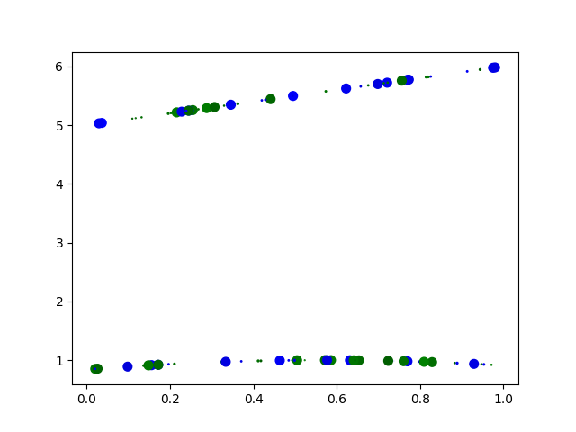
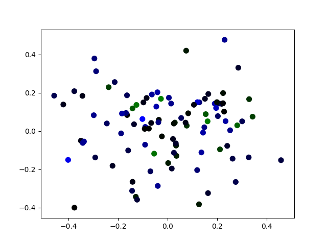
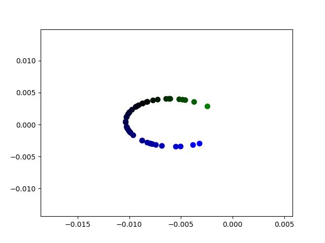
Figure 2. Clustering in ℝ ℝ \mathbb{R} μ = 10 𝜇 10 \mu=10 σ 2 = 1 superscript 𝜎 2 1 \sigma^{2}=1
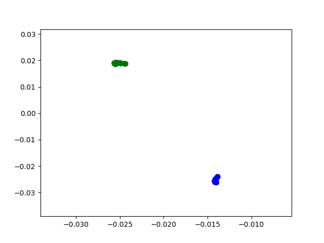
3.2. Mixture of two components in ℝ ℝ \mathbb{R}
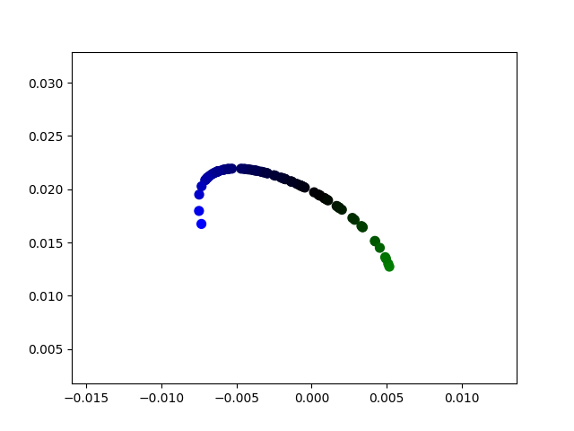
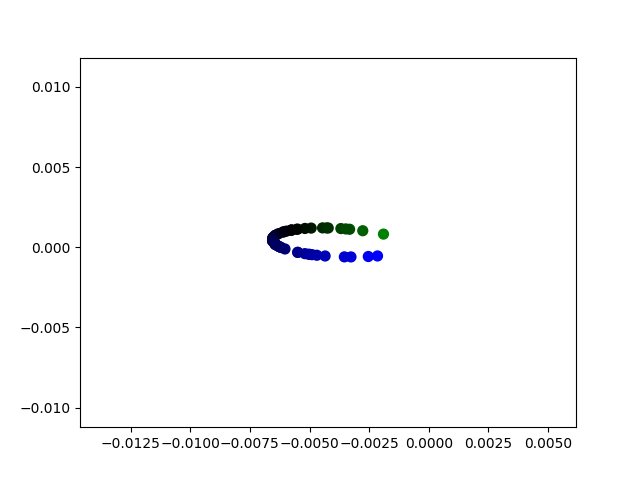
Fig. 3 μ 1 = − 5 subscript 𝜇 1 5 \mu_{1}=-5 μ 2 = 5 subscript 𝜇 2 5 \mu_{2}=5 σ 1 2 = 0.1 superscript subscript 𝜎 1 2 0.1 \sigma_{1}^{2}=0.1 σ 2 2 = 0.1 superscript subscript 𝜎 2 2 0.1 \sigma_{2}^{2}=0.1 between
groups is large compared to the distance within each group).
Figure 3. Clustering in ℝ ℝ \mathbb{R} μ 1 = − 5 subscript 𝜇 1 5 \mu_{1}=-5 μ 2 = 5 subscript 𝜇 2 5 \mu_{2}=5 σ 1 2 = 0.1 superscript subscript 𝜎 1 2 0.1 \sigma_{1}^{2}=0.1 σ 2 2 = 0.1 superscript subscript 𝜎 2 2 0.1 \sigma_{2}^{2}=0.1
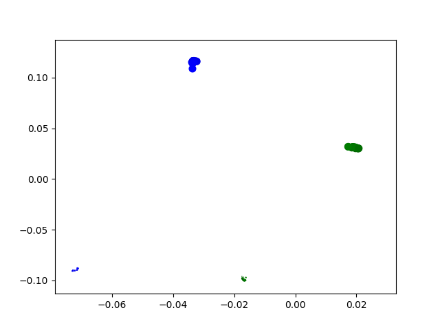
3.3. Single component in ℝ 2 superscript ℝ 2 \mathbb{R}^{2}
Besides color, one could also measure, for instance, size.
These measures could have weights, reflected in the
kernel
K i , j = e α 1 ( c i − c j ) 2 + α 2 ( s i − s j ) 2 subscript 𝐾 𝑖 𝑗
superscript 𝑒 subscript 𝛼 1 superscript subscript 𝑐 𝑖 subscript 𝑐 𝑗 2 subscript 𝛼 2 superscript subscript 𝑠 𝑖 subscript 𝑠 𝑗 2 K_{i,j}=e^{\alpha_{1}(c_{i}-c_{j})^{2}+\alpha_{2}(s_{i}-s_{j})^{2}}
where α 1 , α 2 ∈ ℝ + subscript 𝛼 1 subscript 𝛼 2
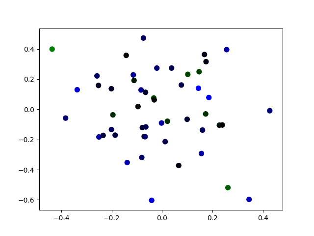
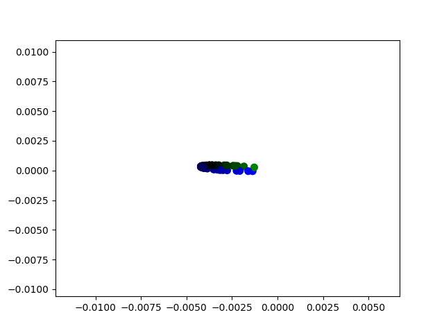
subscript ℝ \alpha_{1},\alpha_{2}\in\mathbb{R}_{+} 4 μ 1 = 20 subscript 𝜇 1 20 \mu_{1}=20 σ 1 2 = 1 superscript subscript 𝜎 1 2 1 \sigma_{1}^{2}=1 μ 2 = 10 subscript 𝜇 2 10 \mu_{2}=10 σ 2 2 = 0.1 superscript subscript 𝜎 2 2 0.1 \sigma_{2}^{2}=0.1 α 1 subscript 𝛼 1 \alpha_{1} α 2 subscript 𝛼 2 \alpha_{2} α 1 = 0.0001 subscript 𝛼 1 0.0001 \alpha_{1}=0.0001 α 2 = 1 subscript 𝛼 2 1 \alpha_{2}=1
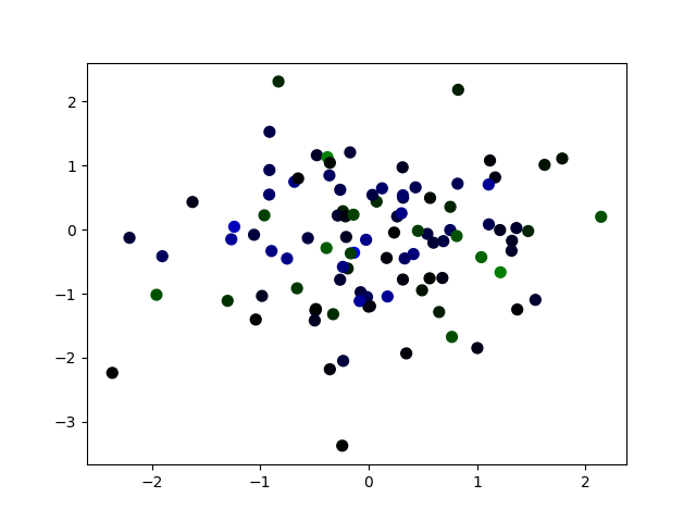
Figure 4. Clustering in ℝ 2 superscript ℝ 2 \mathbb{R}^{2} μ 1 = 20 subscript 𝜇 1 20 \mu_{1}=20 σ 1 2 = 1 superscript subscript 𝜎 1 2 1 \sigma_{1}^{2}=1 μ 2 = 10 subscript 𝜇 2 10 \mu_{2}=10 σ 2 2 = 0.1 superscript subscript 𝜎 2 2 0.1 \sigma_{2}^{2}=0.1 α 1 = 0.0001 subscript 𝛼 1 0.0001 \alpha_{1}=0.0001 α 2 = 1 subscript 𝛼 2 1 \alpha_{2}=1 α 2 ≫ α 1 much-greater-than subscript 𝛼 2 subscript 𝛼 1 \alpha_{2}\gg\alpha_{1}
3.4. Mixture of two components in ℝ 2 superscript ℝ 2 \mathbb{R}^{2}
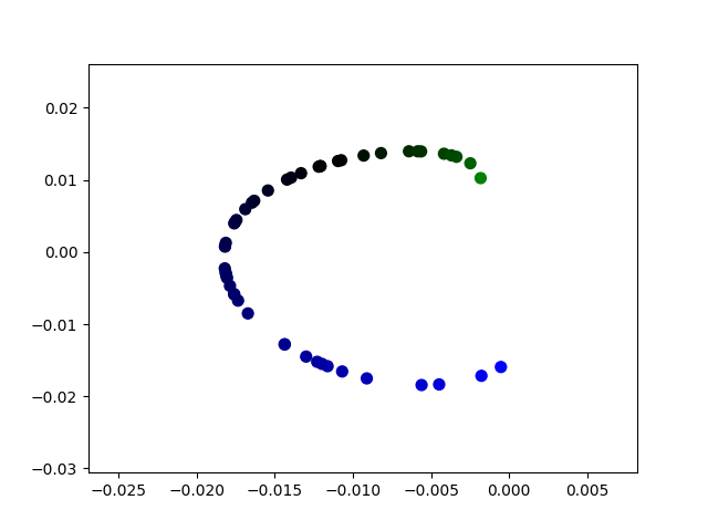
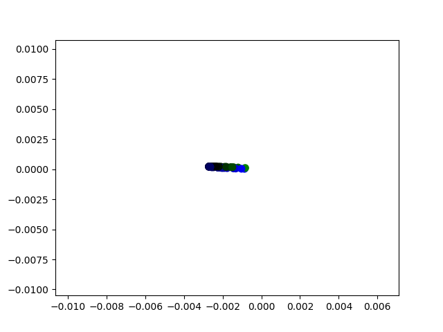
Fig. 5 ℝ 2 superscript ℝ 2 \mathbb{R}^{2} μ 1 = − 20 subscript 𝜇 1 20 \mu_{1}=-20 μ 2 = 20 subscript 𝜇 2 20 \mu_{2}=20 σ 1 2 = 1 superscript subscript 𝜎 1 2 1 \sigma_{1}^{2}=1 σ 2 2 = 1 superscript subscript 𝜎 2 2 1 \sigma_{2}^{2}=1 μ 3 = 10 subscript 𝜇 3 10 \mu_{3}=10 μ 4 = 20 subscript 𝜇 4 20 \mu_{4}=20 σ 3 2 = 0.1 superscript subscript 𝜎 3 2 0.1 \sigma_{3}^{2}=0.1 σ 4 2 = 0.1 superscript subscript 𝜎 4 2 0.1 \sigma_{4}^{2}=0.1 α 1 = 0.01 subscript 𝛼 1 0.01 \alpha_{1}=0.01 α 2 = 1 subscript 𝛼 2 1 \alpha_{2}=1
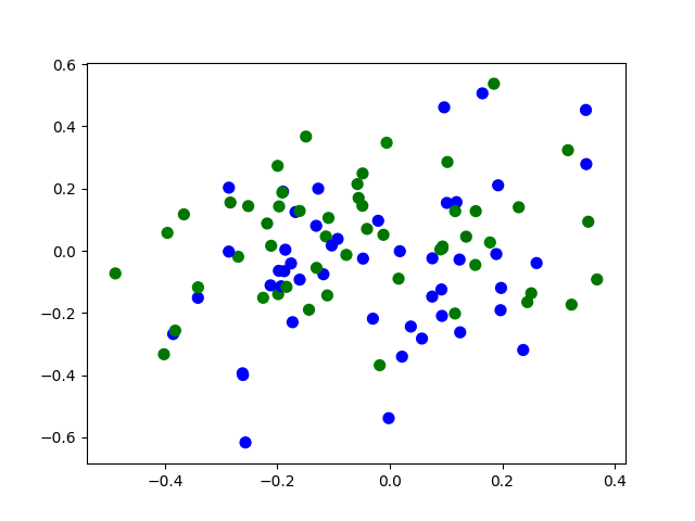
Figure 5. Clustering in ℝ 2 superscript ℝ 2 \mathbb{R}^{2} μ 1 = − 20 subscript 𝜇 1 20 \mu_{1}=-20 μ 2 = 20 subscript 𝜇 2 20 \mu_{2}=20 σ 1 2 = 1 superscript subscript 𝜎 1 2 1 \sigma_{1}^{2}=1 σ 2 2 = 1 superscript subscript 𝜎 2 2 1 \sigma_{2}^{2}=1 μ 3 = 10 subscript 𝜇 3 10 \mu_{3}=10 μ 4 = 20 subscript 𝜇 4 20 \mu_{4}=20 σ 3 2 = 0.1 superscript subscript 𝜎 3 2 0.1 \sigma_{3}^{2}=0.1 σ 4 2 = 0.1 superscript subscript 𝜎 4 2 0.1 \sigma_{4}^{2}=0.1 α 1 = 0.01 subscript 𝛼 1 0.01 \alpha_{1}=0.01 α 2 = 1 subscript 𝛼 2 1 \alpha_{2}=1
3.5. Clustering of lines or shapes
The clustering seems (more or less) independent of the initial
shapes. Sometimes objects
may be placed on lines (underlying clusters themselves), but
the resulting clustering is not affected.
Fig. 6 ℝ 2 superscript ℝ 2 \mathbb{R}^{2} μ 1 = − 20 subscript 𝜇 1 20 \mu_{1}=-20 μ 2 = 20 subscript 𝜇 2 20 \mu_{2}=20 σ 1 2 = 1 superscript subscript 𝜎 1 2 1 \sigma_{1}^{2}=1 σ 2 2 = 1 superscript subscript 𝜎 2 2 1 \sigma_{2}^{2}=1 μ 3 = 10 subscript 𝜇 3 10 \mu_{3}=10 μ 4 = 20 subscript 𝜇 4 20 \mu_{4}=20 σ 3 2 = 0.1 superscript subscript 𝜎 3 2 0.1 \sigma_{3}^{2}=0.1 σ 4 2 = 0.1 superscript subscript 𝜎 4 2 0.1 \sigma_{4}^{2}=0.1 α 1 = 0.01 subscript 𝛼 1 0.01 \alpha_{1}=0.01 α 2 = 1 subscript 𝛼 2 1 \alpha_{2}=1
Figure 6. Clustering of lines in ℝ 2 superscript ℝ 2 \mathbb{R}^{2} μ 1 = − 20 subscript 𝜇 1 20 \mu_{1}=-20 μ 2 = 20 subscript 𝜇 2 20 \mu_{2}=20 σ 1 2 = 1 superscript subscript 𝜎 1 2 1 \sigma_{1}^{2}=1 σ 2 2 = 1 superscript subscript 𝜎 2 2 1 \sigma_{2}^{2}=1 μ 3 = 10 subscript 𝜇 3 10 \mu_{3}=10 μ 4 = 20 subscript 𝜇 4 20 \mu_{4}=20 σ 3 2 = 0.1 superscript subscript 𝜎 3 2 0.1 \sigma_{3}^{2}=0.1 σ 4 2 = 0.1 superscript subscript 𝜎 4 2 0.1 \sigma_{4}^{2}=0.1 α 1 = 0.01 subscript 𝛼 1 0.01 \alpha_{1}=0.01 α 2 = 1 subscript 𝛼 2 1 \alpha_{2}=1
3.6. Mixture of two components in ℝ ℝ \mathbb{R}
As an adaptation of the original model we suggest the following
redefinition of the kernel,
(11) K i , j = e − 1 σ n ‖ x i − x j ‖ 2 / ω 2 n , subscript 𝐾 𝑖 𝑗
superscript 𝑒 1 𝜎 𝑛 superscript norm subscript 𝑥 𝑖 subscript 𝑥 𝑗 2 superscript 𝜔 2 𝑛 \displaystyle K_{i,j}=\frac{e^{-\frac{1}{\sigma n}\|x_{i}-x_{j}\|^{2}/\omega^{2}}}{n},
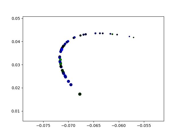
where σ = max ( σ 1 , … , σ l ) 𝜎 subscript 𝜎 1 … subscript 𝜎 𝑙 \sigma=\max(\sigma_{1},\ldots,\sigma_{l}) 7 μ 1 = − 10 subscript 𝜇 1 10 \mu_{1}=-10 μ 2 = 10 subscript 𝜇 2 10 \mu_{2}=10 σ 1 = 10 subscript 𝜎 1 10 \sigma_{1}=10 σ 2 = 10 subscript 𝜎 2 10 \sigma_{2}=10 σ n 𝜎 𝑛 \sigma n 8 11
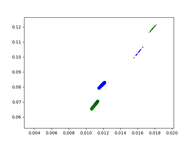
Figure 7. Clustering in ℝ ℝ \mathbb{R} μ 1 = − 10 subscript 𝜇 1 10 \mu_{1}=-10 μ 2 = 10 subscript 𝜇 2 10 \mu_{2}=10 σ 1 2 = 10 superscript subscript 𝜎 1 2 10 \sigma_{1}^{2}=10 σ 2 2 = 10 superscript subscript 𝜎 2 2 10 \sigma_{2}^{2}=10
Figure 8. Clustering in ℝ ℝ \mathbb{R} μ 1 = − 10 subscript 𝜇 1 10 \mu_{1}=-10 μ 2 = 10 subscript 𝜇 2 10 \mu_{2}=10 σ 1 2 = 10 superscript subscript 𝜎 1 2 10 \sigma_{1}^{2}=10 σ 2 2 = 10 superscript subscript 𝜎 2 2 10 \sigma_{2}^{2}=10
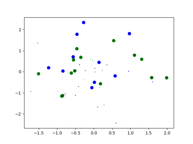
4. Example of the main theorem
In the following section we illustrate the main theorem (see Table 1 λ 0 = 0.62 subscript 𝜆 0 0.62 \lambda_{0}=0.62 λ 1 = 0.22 subscript 𝜆 1 0.22 \lambda_{1}=0.22 λ 2 = 0.08 subscript 𝜆 2 0.08 \lambda_{2}=0.08 Main theorem: Second leading eigenvalue of mixture distribution ( 0.18 , 0.33 ) 0.18 0.33 (0.18,0.33) λ 1 subscript 𝜆 1 \lambda_{1} λ 0 subscript 𝜆 0 \lambda_{0} λ 2 subscript 𝜆 2 \lambda_{2}
In the provided example
π 1 subscript 𝜋 1 \pi_{1} π 2 subscript 𝜋 2 \pi_{2} π 1 subscript 𝜋 1 \pi_{1} π 1 subscript 𝜋 1 \pi_{1} ‖ δ ‖ norm 𝛿 \|\delta\|
Fig. 9 1
Since the dynamical system T x subscript 𝑇 𝑥 T_{x} y 𝑦 y Main theorem: Second leading eigenvalue of mixture distribution λ 0 subscript 𝜆 0 \lambda_{0} T x subscript 𝑇 𝑥 T_{x} 𝒦 = K ⊗ K 𝒦 tensor-product 𝐾 𝐾 \mathcal{K}=K\otimes K 9
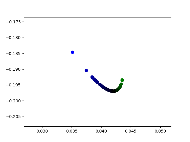
Table 1. Simulation parameters for exemplifying Theorem Main theorem: Second leading eigenvalue of mixture distribution
Figure 9. Clustering with parameters as in Table 1
5. Conclusions and further work
We have described a particular algorithm which treats a collection of elements of an image as a certain dynamical system. As input we use a Gaussian mixture distribution of several components. The clustering seems efficient when compared to its overall simplicity. As described, the algorithm preserves, or, respects the underlying data structure. In general the clustering seems satisfactory given that the deviation of components is not too high as compared to the sizes of the standard deviations. As an adaptation, we suggest a certain redefined model less sensitive to high deviations in the Gaussian mixture distributions. This algorithm produces remarkably efficient clustering even if the components of the mixture distribution are not well isolated (that is the standard deviations are comparable in size to the difference between the means).
We also construct bounds for the second largest eigenvalue of the kernel matrix used in the algorithm for a Gaussian mixture P = π 1 P 1 + π 2 P 2 𝑃 subscript 𝜋 1 superscript 𝑃 1 subscript 𝜋 2 superscript 𝑃 2 P=\pi_{1}P^{1}+\pi_{2}P^{2} π 1 subscript 𝜋 1 \pi_{1} Main theorem: Second leading eigenvalue of mixture distribution 1.9 T x ( y ) subscript 𝑇 𝑥 𝑦 T_{x}(y)
6. Appendix
Calculating 𝒓 𝒓 \bm{r}
r 𝑟 \displaystyle r = \displaystyle= ( π 1 π 2 ∬ K ( x , y ) 2 𝑑 P 1 ( x ) 𝑑 P 2 ( y ) ) 1 / 2 superscript subscript 𝜋 1 subscript 𝜋 2 double-integral 𝐾 superscript 𝑥 𝑦 2 differential-d superscript 𝑃 1 𝑥 differential-d superscript 𝑃 2 𝑦 1 2 \displaystyle(\pi_{1}\pi_{2}\iint K(x,y)^{2}dP^{1}(x)dP^{2}(y))^{1/2}
= \displaystyle= ( π 1 π 2 π ω 4 σ 1 2 + 4 σ 2 2 + ω 2 e − 2 ( μ 1 + μ 2 ) 2 4 σ 1 2 + 4 σ 2 2 + ω 2 ) 1 2 superscript subscript 𝜋 1 subscript 𝜋 2 𝜋 𝜔 4 superscript subscript 𝜎 1 2 4 superscript subscript 𝜎 2 2 superscript 𝜔 2 superscript 𝑒 2 superscript subscript 𝜇 1 subscript 𝜇 2 2 4 superscript subscript 𝜎 1 2 4 superscript subscript 𝜎 2 2 superscript 𝜔 2 1 2 \displaystyle\left(\pi_{1}\pi_{2}{\pi\omega\over\sqrt{4\sigma_{1}^{2}+4\sigma_{2}^{2}+\omega^{2}}}e^{-{2(\mu_{1}+\mu_{2})^{2}\over 4\sigma_{1}^{2}+4\sigma_{2}^{2}+\omega^{2}}}\right)^{1\over 2}
= \displaystyle= π 1 π 2 π ω ( 4 σ 1 2 + 4 σ 2 2 + ω 2 ) 1 4 e − ( μ 1 + μ 2 ) 2 4 σ 1 2 + 4 σ 2 2 + ω 2 . subscript 𝜋 1 subscript 𝜋 2 𝜋 𝜔 superscript 4 superscript subscript 𝜎 1 2 4 superscript subscript 𝜎 2 2 superscript 𝜔 2 1 4 superscript 𝑒 superscript subscript 𝜇 1 subscript 𝜇 2 2 4 superscript subscript 𝜎 1 2 4 superscript subscript 𝜎 2 2 superscript 𝜔 2 \displaystyle\sqrt{\pi_{1}\pi_{2}}{\sqrt{\pi\omega}\over\left(4\sigma_{1}^{2}+4\sigma_{2}^{2}+\omega^{2}\right)^{1\over 4}}e^{-{(\mu_{1}+\mu_{2})^{2}\over 4\sigma_{1}^{2}+4\sigma_{2}^{2}+\omega^{2}}}.
Calculating ‖ 𝑲 ‖ 𝑳 𝑷 𝟐 𝟐 × 𝑳 𝑷 𝟐 subscript norm 𝑲 subscript superscript 𝑳 2 superscript 𝑷 2 subscript superscript 𝑳 2 𝑷 \bm{\left\|K\right\|_{L^{2}_{P^{2}}\times L^{2}_{P}}}
∬ K ( x , z ) 2 𝑑 P 2 ( x ) 𝑑 P ( z ) double-integral 𝐾 superscript 𝑥 𝑧 2 differential-d superscript 𝑃 2 𝑥 differential-d 𝑃 𝑧 \displaystyle\iint K(x,z)^{2}dP^{2}(x)dP(z) = π 1 ∬ K ( x , z ) 2 𝑑 P 2 ( x ) 𝑑 P 1 ( z ) + absent limit-from subscript 𝜋 1 double-integral 𝐾 superscript 𝑥 𝑧 2 differential-d superscript 𝑃 2 𝑥 differential-d superscript 𝑃 1 𝑧 \displaystyle=\pi_{1}\iint K(x,z)^{2}dP^{2}(x)dP^{1}(z)+
+ π 2 ∬ K ( x , z ) 2 𝑑 P 2 ( x ) 𝑑 P 2 ( z ) subscript 𝜋 2 double-integral 𝐾 superscript 𝑥 𝑧 2 differential-d superscript 𝑃 2 𝑥 differential-d superscript 𝑃 2 𝑧 \displaystyle\hskip 20.0pt+\pi_{2}\iint K(x,z)^{2}dP^{2}(x)dP^{2}(z)
= π 1 π ω 4 σ 1 2 + 4 σ 2 2 + ω 2 e − 2 ( μ 1 + μ 2 ) 2 4 σ 1 2 + 4 σ 2 2 + ω 2 + absent limit-from subscript 𝜋 1 𝜋 𝜔 4 superscript subscript 𝜎 1 2 4 superscript subscript 𝜎 2 2 superscript 𝜔 2 superscript 𝑒 2 superscript subscript 𝜇 1 subscript 𝜇 2 2 4 superscript subscript 𝜎 1 2 4 superscript subscript 𝜎 2 2 superscript 𝜔 2 \displaystyle=\pi_{1}{\pi\omega\over\sqrt{4\sigma_{1}^{2}+4\sigma_{2}^{2}+\omega^{2}}}e^{-{2(\mu_{1}+\mu_{2})^{2}\over 4\sigma_{1}^{2}+4\sigma_{2}^{2}+\omega^{2}}}+
+ π 2 π ω 8 σ 2 2 + ω 2 e − 8 μ 2 2 8 σ 2 2 + ω 2 . subscript 𝜋 2 𝜋 𝜔 8 superscript subscript 𝜎 2 2 superscript 𝜔 2 superscript 𝑒 8 superscript subscript 𝜇 2 2 8 superscript subscript 𝜎 2 2 superscript 𝜔 2 \displaystyle\hskip 20.0pt+\pi_{2}{\pi\omega\over\sqrt{8\sigma_{2}^{2}+\omega^{2}}}e^{-{8\mu_{2}^{2}\over 8\sigma_{2}^{2}+\omega^{2}}}.
Calculating ‖ ϕ 𝟏 𝟏 ‖ 𝑷 𝟐 subscript norm superscript subscript bold-italic-ϕ 1 1 superscript 𝑷 2 \bm{\|\phi_{1}^{1}\|_{P^{2}}}
∫ ϕ 1 1 ( x ) 2 𝑑 P 2 ( x ) = ∫ A 0 e − A 1 ( x − μ 1 ) 2 H 1 ( A 2 x − μ 1 σ 1 ) 2 e − A 3 ( x − μ 2 ) 2 𝑑 x , superscript subscript italic-ϕ 1 1 superscript 𝑥 2 differential-d superscript 𝑃 2 𝑥 subscript 𝐴 0 superscript 𝑒 subscript 𝐴 1 superscript 𝑥 subscript 𝜇 1 2 subscript 𝐻 1 superscript subscript 𝐴 2 𝑥 subscript 𝜇 1 subscript 𝜎 1 2 superscript 𝑒 subscript 𝐴 3 superscript 𝑥 subscript 𝜇 2 2 differential-d 𝑥 \displaystyle\int\phi_{1}^{1}(x)^{2}dP^{2}(x)=\int A_{0}e^{-A_{1}(x-\mu_{1})^{2}}H_{1}\left(A_{2}\frac{x-\mu_{1}}{\sigma_{1}}\right)^{2}e^{-A_{3}(x-\mu_{2})^{2}}dx,
where
A 0 = ( 1 + 2 β ∗ ) 1 / 4 2 2 π σ 2 2 , A 1 = 1 + 2 β ∗ − 1 2 σ 1 2 , A 2 = ( 1 + 2 β ∗ 4 ) 1 / 4 , A 3 = 1 2 σ 2 2 , formulae-sequence subscript 𝐴 0 superscript 1 2 superscript 𝛽 1 4 2 2 𝜋 superscript subscript 𝜎 2 2 formulae-sequence subscript 𝐴 1 1 2 superscript 𝛽 1 2 superscript subscript 𝜎 1 2 formulae-sequence subscript 𝐴 2 superscript 1 2 superscript 𝛽 4 1 4 subscript 𝐴 3 1 2 superscript subscript 𝜎 2 2 A_{0}=\frac{(1+2\beta^{*})^{1/4}}{2\sqrt{2\pi\sigma_{2}^{2}}},\quad A_{1}=\frac{\sqrt{1+2\beta^{*}}-1}{2\sigma_{1}^{2}},\quad A_{2}=\left(\frac{1+2\beta^{*}}{4}\right)^{1/4},\quad A_{3}=\frac{1}{2\sigma_{2}^{2}},
and β ∗ = 2 σ 1 2 / ω 2 superscript 𝛽 2 superscript subscript 𝜎 1 2 superscript 𝜔 2 \beta^{*}=2\sigma_{1}^{2}/\omega^{2}
− A 1 ( x − μ 1 ) 2 − A 3 ( x − μ 2 ) 2 subscript 𝐴 1 superscript 𝑥 subscript 𝜇 1 2 subscript 𝐴 3 superscript 𝑥 subscript 𝜇 2 2 \displaystyle-A_{1}(x-\mu_{1})^{2}-A_{3}(x-\mu_{2})^{2}
= − A 1 ( x 2 − 2 x μ 1 + μ 1 2 ) − A 3 ( x 2 − 2 x μ 2 + μ 2 2 ) absent subscript 𝐴 1 superscript 𝑥 2 2 𝑥 subscript 𝜇 1 superscript subscript 𝜇 1 2 subscript 𝐴 3 superscript 𝑥 2 2 𝑥 subscript 𝜇 2 superscript subscript 𝜇 2 2 \displaystyle\hskip 20.0pt=-A_{1}(x^{2}-2x\mu_{1}+\mu_{1}^{2})-A_{3}(x^{2}-2x\mu_{2}+\mu_{2}^{2})
= − ( A 1 + A 3 ) x 2 + ( 2 μ 1 A 1 + 2 μ 2 A 3 ) x − A 1 μ 1 2 − A 3 μ 2 2 absent subscript 𝐴 1 subscript 𝐴 3 superscript 𝑥 2 2 subscript 𝜇 1 subscript 𝐴 1 2 subscript 𝜇 2 subscript 𝐴 3 𝑥 subscript 𝐴 1 superscript subscript 𝜇 1 2 subscript 𝐴 3 superscript subscript 𝜇 2 2 \displaystyle\hskip 20.0pt=-(A_{1}+A_{3})x^{2}+(2\mu_{1}A_{1}+2\mu_{2}A_{3})x-A_{1}\mu_{1}^{2}-A_{3}\mu_{2}^{2}
= − ( A 1 + A 3 ) ( x 2 − 2 μ 1 A 1 + μ 2 A 3 A 1 + A 3 x + A 1 μ 1 2 + A 3 μ 2 2 A 1 + A 3 ) absent subscript 𝐴 1 subscript 𝐴 3 superscript 𝑥 2 2 subscript 𝜇 1 subscript 𝐴 1 subscript 𝜇 2 subscript 𝐴 3 subscript 𝐴 1 subscript 𝐴 3 𝑥 subscript 𝐴 1 superscript subscript 𝜇 1 2 subscript 𝐴 3 superscript subscript 𝜇 2 2 subscript 𝐴 1 subscript 𝐴 3 \displaystyle\hskip 20.0pt=-(A_{1}+A_{3})\left(x^{2}-2\frac{\mu_{1}A_{1}+\mu_{2}A_{3}}{A_{1}+A_{3}}x+\frac{A_{1}\mu_{1}^{2}+A_{3}\mu_{2}^{2}}{A_{1}+A_{3}}\right)
= − ( A 1 + A 3 ) [ ( x − μ 1 A 1 + μ 2 A 3 A 1 + A 3 ) 2 − ( μ 1 A 1 + μ 2 A 3 A 1 + A 3 ) 2 + \displaystyle\hskip 20.0pt=-(A_{1}+A_{3})\left[\left(x-\frac{\mu_{1}A_{1}+\mu_{2}A_{3}}{A_{1}+A_{3}}\right)^{2}-\left(\frac{\mu_{1}A_{1}+\mu_{2}A_{3}}{A_{1}+A_{3}}\right)^{2}+\right.
+ A 1 μ 1 2 + A 3 μ 2 2 A 1 + A 3 ] \displaystyle\hskip 218.0pt\left.+\frac{A_{1}\mu_{1}^{2}+A_{3}\mu_{2}^{2}}{A_{1}+A_{3}}\right]
= − a [ ( x − b ) 2 + c ] absent 𝑎 delimited-[] superscript 𝑥 𝑏 2 𝑐 \displaystyle\hskip 20.0pt=-a\left[(x-b)^{2}+c\right]
with a 𝑎 a b 𝑏 b c 𝑐 c
A 0 ∫ ϕ 1 1 ( x ) 2 𝑑 P 2 ( x ) subscript 𝐴 0 superscript subscript italic-ϕ 1 1 superscript 𝑥 2 differential-d superscript 𝑃 2 𝑥 \displaystyle A_{0}\int\phi_{1}^{1}(x)^{2}dP^{2}(x) = A 0 ∫ e − a ( ( x − b ) 2 + c ) H 1 ( A 2 x − μ 1 σ 1 ) 2 𝑑 x absent subscript 𝐴 0 superscript 𝑒 𝑎 superscript 𝑥 𝑏 2 𝑐 subscript 𝐻 1 superscript subscript 𝐴 2 𝑥 subscript 𝜇 1 subscript 𝜎 1 2 differential-d 𝑥 \displaystyle=A_{0}\int e^{-a((x-b)^{2}+c)}H_{1}\left(A_{2}\frac{x-\mu_{1}}{\sigma_{1}}\right)^{2}dx
= A 0 e − a c ∫ e − a ( x − b ) 2 H 1 ( A 2 x − μ 1 σ 1 ) 2 𝑑 x absent subscript 𝐴 0 superscript 𝑒 𝑎 𝑐 superscript 𝑒 𝑎 superscript 𝑥 𝑏 2 subscript 𝐻 1 superscript subscript 𝐴 2 𝑥 subscript 𝜇 1 subscript 𝜎 1 2 differential-d 𝑥 \displaystyle=A_{0}e^{-ac}\int e^{-a(x-b)^{2}}H_{1}\left(A_{2}\frac{x-\mu_{1}}{\sigma_{1}}\right)^{2}dx
= A 0 σ 1 A 2 e − a c ∫ e − a ( σ 1 y A 2 + μ 1 − b ) 2 H 1 2 ( y ) 𝑑 y absent subscript 𝐴 0 subscript 𝜎 1 subscript 𝐴 2 superscript 𝑒 𝑎 𝑐 superscript 𝑒 𝑎 superscript subscript 𝜎 1 𝑦 subscript 𝐴 2 subscript 𝜇 1 𝑏 2 superscript subscript 𝐻 1 2 𝑦 differential-d 𝑦 \displaystyle=A_{0}\frac{\sigma_{1}}{A_{2}}e^{-ac}\int e^{-a\left(\frac{\sigma_{1}y}{A_{2}}+\mu_{1}-b\right)^{2}}H_{1}^{2}(y)dy
= A 0 σ 1 A 2 e − a c ∫ e − a σ 1 2 A 2 2 ( y − A 2 b − μ 1 σ 1 ) 2 H 1 2 ( y ) 𝑑 y . absent subscript 𝐴 0 subscript 𝜎 1 subscript 𝐴 2 superscript 𝑒 𝑎 𝑐 superscript 𝑒 𝑎 superscript subscript 𝜎 1 2 superscript subscript 𝐴 2 2 superscript 𝑦 subscript 𝐴 2 𝑏 subscript 𝜇 1 subscript 𝜎 1 2 superscript subscript 𝐻 1 2 𝑦 differential-d 𝑦 \displaystyle=A_{0}\frac{\sigma_{1}}{A_{2}}e^{-ac}\int e^{-a\frac{\sigma_{1}^{2}}{A_{2}^{2}}\left(y-A_{2}\frac{b-\mu_{1}}{\sigma_{1}}\right)^{2}}H_{1}^{2}(y)dy.
Let x ~ = A 2 ( b − μ 1 ) / σ 1 ~ 𝑥 subscript 𝐴 2 𝑏 subscript 𝜇 1 subscript 𝜎 1 \tilde{x}=A_{2}(b-\mu_{1})/{\sigma_{1}} R = a σ 1 2 / A 2 2 𝑅 𝑎 superscript subscript 𝜎 1 2 superscript subscript 𝐴 2 2 R=a\sigma_{1}^{2}/A_{2}^{2}
A 0 σ 1 A 2 e − a c ∫ e − R ( y − x ~ ) 2 H 1 2 ( y ) 𝑑 y . subscript 𝐴 0 subscript 𝜎 1 subscript 𝐴 2 superscript 𝑒 𝑎 𝑐 superscript 𝑒 𝑅 superscript 𝑦 ~ 𝑥 2 superscript subscript 𝐻 1 2 𝑦 differential-d 𝑦 A_{0}\frac{\sigma_{1}}{A_{2}}e^{-ac}\int e^{-R\left(y-\tilde{x}\right)^{2}}H_{1}^{2}(y)dy.
Since
∫ e − R ( y − x ~ ) 2 H 1 2 ( y ) 𝑑 y = π ( 2 R x ~ 2 + 1 ) 2 R 3 / 2 , superscript 𝑒 𝑅 superscript 𝑦 ~ 𝑥 2 superscript subscript 𝐻 1 2 𝑦 differential-d 𝑦 𝜋 2 𝑅 superscript ~ 𝑥 2 1 2 superscript 𝑅 3 2 \int e^{-R\left(y-\tilde{x}\right)^{2}}H_{1}^{2}(y)dy=\frac{\sqrt{\pi}(2R\tilde{x}^{2}+1)}{2R^{3/2}},
we get
(12) ∫ ( ϕ 1 1 ( x ) ) 2 𝑑 P 2 ( x ) = A 0 σ 1 A 2 e − a c π ( 2 R x ~ 2 + 1 ) 2 R 3 / 2 . superscript superscript subscript italic-ϕ 1 1 𝑥 2 differential-d superscript 𝑃 2 𝑥 subscript 𝐴 0 subscript 𝜎 1 subscript 𝐴 2 superscript 𝑒 𝑎 𝑐 𝜋 2 𝑅 superscript ~ 𝑥 2 1 2 superscript 𝑅 3 2 \displaystyle\int(\phi_{1}^{1}(x))^{2}dP^{2}(x)=A_{0}\frac{\sigma_{1}}{A_{2}}e^{-ac}\frac{\sqrt{\pi}(2R\tilde{x}^{2}+1)}{2R^{3/2}}.
Note that we have made implicit the assumption R ≥ 0 𝑅 0 R\geq 0
Calculating 𝝀 𝟎 ∫ ϕ 𝟏 𝟏 ( 𝒙 ) ϕ 𝟎 𝟏 ( 𝒙 ) 𝒅 𝑷 ( 𝒙 ) subscript 𝝀 0 superscript subscript bold-italic-ϕ 1 1 𝒙 superscript subscript bold-italic-ϕ 0 1 𝒙 differential-d 𝑷 𝒙 \bm{\lambda_{0}\int\phi_{1}^{1}(x)\phi_{0}^{1}(x)dP(x)}
λ 0 ∫ ϕ 1 1 ( x ) ϕ 0 1 ( x ) 𝑑 P ( x ) subscript 𝜆 0 superscript subscript italic-ϕ 1 1 𝑥 superscript subscript italic-ϕ 0 1 𝑥 differential-d 𝑃 𝑥 \displaystyle\lambda_{0}\int\phi_{1}^{1}(x)\phi_{0}^{1}(x)dP(x)
= λ 0 ∫ π 1 ϕ 1 1 ( x ) ϕ 0 1 ( x ) 𝑑 P 1 ( x ) + λ 0 ∫ π 2 ϕ 1 1 ( x ) ϕ 0 1 ( x ) 𝑑 P 2 ( x ) absent subscript 𝜆 0 subscript 𝜋 1 superscript subscript italic-ϕ 1 1 𝑥 superscript subscript italic-ϕ 0 1 𝑥 differential-d superscript 𝑃 1 𝑥 subscript 𝜆 0 subscript 𝜋 2 superscript subscript italic-ϕ 1 1 𝑥 superscript subscript italic-ϕ 0 1 𝑥 differential-d superscript 𝑃 2 𝑥 \displaystyle\hskip 20.0pt=\lambda_{0}\int\pi_{1}\phi_{1}^{1}(x)\phi_{0}^{1}(x)dP^{1}(x)+\lambda_{0}\int\pi_{2}\phi_{1}^{1}(x)\phi_{0}^{1}(x)dP^{2}(x)
= λ 0 π 2 ∫ ϕ 1 1 ( x ) ϕ 0 1 ( x ) 𝑑 P 2 ( x ) absent subscript 𝜆 0 subscript 𝜋 2 superscript subscript italic-ϕ 1 1 𝑥 superscript subscript italic-ϕ 0 1 𝑥 differential-d superscript 𝑃 2 𝑥 \displaystyle\hskip 20.0pt=\lambda_{0}\pi_{2}\int\phi_{1}^{1}(x)\phi_{0}^{1}(x)dP^{2}(x)
= ∫ B 1 e − B 2 ( x − μ 1 ) 2 H 1 ( B 3 ( x − μ 1 ) ) B 4 e − B 2 ( x − μ 1 ) 2 e − B 5 ( x − μ 2 ) 2 𝑑 x absent subscript 𝐵 1 superscript 𝑒 subscript 𝐵 2 superscript 𝑥 subscript 𝜇 1 2 subscript 𝐻 1 subscript 𝐵 3 𝑥 subscript 𝜇 1 subscript 𝐵 4 superscript 𝑒 subscript 𝐵 2 superscript 𝑥 subscript 𝜇 1 2 superscript 𝑒 subscript 𝐵 5 superscript 𝑥 subscript 𝜇 2 2 differential-d 𝑥 \displaystyle\hskip 20.0pt=\int B_{1}e^{-B_{2}(x-\mu_{1})^{2}}H_{1}\left(B_{3}(x-\mu_{1})\right)B_{4}e^{-B_{2}(x-\mu_{1})^{2}}e^{-B_{5}(x-\mu_{2})^{2}}dx
= B 1 B 4 ∫ e − 2 B 2 ( x − μ 1 ) 2 − B 5 ( x − μ 2 ) 2 H 1 ( B 3 ( x − μ 1 ) ) 𝑑 x , absent subscript 𝐵 1 subscript 𝐵 4 superscript 𝑒 2 subscript 𝐵 2 superscript 𝑥 subscript 𝜇 1 2 subscript 𝐵 5 superscript 𝑥 subscript 𝜇 2 2 subscript 𝐻 1 subscript 𝐵 3 𝑥 subscript 𝜇 1 differential-d 𝑥 \displaystyle\hskip 20.0pt=B_{1}B_{4}\int e^{-2B_{2}(x-\mu_{1})^{2}-B_{5}(x-\mu_{2})^{2}}H_{1}(B_{3}(x-\mu_{1}))dx,
where
B 1 = λ 0 π 2 2 π σ 2 2 ( 1 + 2 β ∗ 2 ) 1 / 8 , B 2 = \displaystyle B_{1}=\frac{\lambda_{0}\pi_{2}}{\sqrt{2\pi\sigma_{2}^{2}}}\left(\frac{1+2\beta^{*}}{\sqrt{2}}\right)^{1/8},\quad B_{2}= 1 + 2 β ∗ − 1 4 σ 1 2 , B 3 = ( 1 + 2 β ∗ 4 ) 1 / 4 , 1 2 superscript 𝛽 1 4 superscript subscript 𝜎 1 2 subscript 𝐵 3
superscript 1 2 superscript 𝛽 4 1 4 \displaystyle\frac{\sqrt{1+2\beta^{*}}-1}{4\sigma_{1}^{2}},\quad B_{3}=\left(\frac{1+2\beta^{*}}{4}\right)^{1/4},
B 4 = ( 1 + 2 β ∗ ) 1 / 8 , subscript 𝐵 4 superscript 1 2 superscript 𝛽 1 8 \displaystyle B_{4}=(1+2\beta^{*})^{1/8}, B 5 = 1 2 σ 2 2 . subscript 𝐵 5 1 2 superscript subscript 𝜎 2 2 \displaystyle\quad B_{5}=\frac{1}{2\sigma_{2}^{2}}.
We have
− 2 B 2 ( x − μ 1 ) 2 − B 5 ( x − μ 2 ) 2 2 subscript 𝐵 2 superscript 𝑥 subscript 𝜇 1 2 subscript 𝐵 5 superscript 𝑥 subscript 𝜇 2 2 \displaystyle-2B_{2}(x-\mu_{1})^{2}-B_{5}(x-\mu_{2})^{2}
= ( − 2 B 2 − B 5 ) x 2 + ( 2 B 2 μ 1 + B 5 μ 2 ) 2 x − 2 B 2 μ 1 2 − B 5 μ 2 2 absent 2 subscript 𝐵 2 subscript 𝐵 5 superscript 𝑥 2 2 subscript 𝐵 2 subscript 𝜇 1 subscript 𝐵 5 subscript 𝜇 2 2 𝑥 2 subscript 𝐵 2 superscript subscript 𝜇 1 2 subscript 𝐵 5 superscript subscript 𝜇 2 2 \displaystyle\hskip 20.0pt=(-2B_{2}-B_{5})x^{2}+(2B_{2}\mu_{1}+B_{5}\mu_{2})2x-2B_{2}\mu_{1}^{2}-B_{5}\mu_{2}^{2}
= ( − 2 B 2 − B 5 ) ( x 2 − 2 2 B 2 μ 1 + B 5 μ 2 2 B 2 + B 5 x + 2 B 2 μ 1 2 + B 5 μ 2 2 2 B 2 + B 5 ) absent 2 subscript 𝐵 2 subscript 𝐵 5 superscript 𝑥 2 2 2 subscript 𝐵 2 subscript 𝜇 1 subscript 𝐵 5 subscript 𝜇 2 2 subscript 𝐵 2 subscript 𝐵 5 𝑥 2 subscript 𝐵 2 superscript subscript 𝜇 1 2 subscript 𝐵 5 superscript subscript 𝜇 2 2 2 subscript 𝐵 2 subscript 𝐵 5 \displaystyle\hskip 20.0pt=(-2B_{2}-B_{5})\left(x^{2}-2\frac{2B_{2}\mu_{1}+B_{5}\mu_{2}}{2B_{2}+B_{5}}x+\frac{2B_{2}\mu_{1}^{2}+B_{5}\mu_{2}^{2}}{2B_{2}+B_{5}}\right)
= ( − 2 B 2 − B 5 ) [ ( x − 2 B 2 μ 1 + B 5 μ 2 2 B 2 + B 5 ) 2 − ( 2 B 2 μ 1 + B 5 μ 2 2 B 2 + B 5 ) 2 + \displaystyle\hskip 20.0pt=(-2B_{2}-B_{5})\left[\left(x-\frac{2B_{2}\mu_{1}+B_{5}\mu_{2}}{2B_{2}+B_{5}}\right)^{2}-\left(\frac{2B_{2}\mu_{1}+B_{5}\mu_{2}}{2B_{2}+B_{5}}\right)^{2}+\right.
+ 2 B 2 μ 1 2 + B 5 μ 2 2 2 B 2 + B 5 ] \displaystyle\hskip 228.0pt\left.+\frac{2B_{2}\mu_{1}^{2}+B_{5}\mu_{2}^{2}}{2B_{2}+B_{5}}\right]
= − d ( ( x − e ) 2 + f ) , absent 𝑑 superscript 𝑥 𝑒 2 𝑓 \displaystyle\hskip 20.0pt=-d((x-e)^{2}+f),
where d 𝑑 d e 𝑒 e f 𝑓 f
λ 0 ∫ ϕ 1 1 ( x ) ϕ 0 1 ( y ) 𝑑 P ( x ) subscript 𝜆 0 superscript subscript italic-ϕ 1 1 𝑥 superscript subscript italic-ϕ 0 1 𝑦 differential-d 𝑃 𝑥 \displaystyle\lambda_{0}\int\phi_{1}^{1}(x)\phi_{0}^{1}(y)dP(x) = B 1 B 4 e − d f ∫ e − d ( x − e ) 2 H 1 ( B 3 ( x − μ 1 ) ) 𝑑 x absent subscript 𝐵 1 subscript 𝐵 4 superscript 𝑒 𝑑 𝑓 superscript 𝑒 𝑑 superscript 𝑥 𝑒 2 subscript 𝐻 1 subscript 𝐵 3 𝑥 subscript 𝜇 1 differential-d 𝑥 \displaystyle=B_{1}B_{4}e^{-df}\int e^{-d(x-e)^{2}}H_{1}(B_{3}(x-\mu_{1}))dx
= B 1 B 4 B 3 e − d f ∫ e − d ( y B 3 + μ 1 − e ) 2 H 1 ( y ) 𝑑 y absent subscript 𝐵 1 subscript 𝐵 4 subscript 𝐵 3 superscript 𝑒 𝑑 𝑓 superscript 𝑒 𝑑 superscript 𝑦 subscript 𝐵 3 subscript 𝜇 1 𝑒 2 subscript 𝐻 1 𝑦 differential-d 𝑦 \displaystyle={B_{1}B_{4}\over B_{3}}e^{-df}\int e^{-d\left(\frac{y}{B_{3}}+\mu_{1}-e\right)^{2}}H_{1}(y)dy
= B 1 B 4 B 3 e − d f ∫ e − d B 3 2 ( y + B 3 μ 1 − e B 3 ) 2 H 1 ( y ) 𝑑 y absent subscript 𝐵 1 subscript 𝐵 4 subscript 𝐵 3 superscript 𝑒 𝑑 𝑓 superscript 𝑒 𝑑 superscript subscript 𝐵 3 2 superscript 𝑦 subscript 𝐵 3 subscript 𝜇 1 𝑒 subscript 𝐵 3 2 subscript 𝐻 1 𝑦 differential-d 𝑦 \displaystyle={B_{1}B_{4}\over B_{3}}e^{-df}\int e^{-\frac{d}{B_{3}^{2}}\left(y+B_{3}\mu_{1}-eB_{3}\right)^{2}}H_{1}(y)dy
= B 1 B 4 B 3 e − d f ∫ e − d B 3 2 ( y − x ^ ) 2 H 1 ( y ) 𝑑 y absent subscript 𝐵 1 subscript 𝐵 4 subscript 𝐵 3 superscript 𝑒 𝑑 𝑓 superscript 𝑒 𝑑 superscript subscript 𝐵 3 2 superscript 𝑦 ^ 𝑥 2 subscript 𝐻 1 𝑦 differential-d 𝑦 \displaystyle={B_{1}B_{4}\over B_{3}}e^{-df}\int e^{-\frac{d}{B_{3}^{2}}\left(y-\hat{x}\right)^{2}}H_{1}(y)dy
with x ^ ^ 𝑥 \hat{x}
Let S := d / B 3 2 assign 𝑆 𝑑 superscript subscript 𝐵 3 2 S:=d/B_{3}^{2}
∫ e − S ( y − x ^ ) 2 H 1 ( y ) 𝑑 y = π S x ^ , superscript 𝑒 𝑆 superscript 𝑦 ^ 𝑥 2 subscript 𝐻 1 𝑦 differential-d 𝑦 𝜋 𝑆 ^ 𝑥 \displaystyle\int e^{-S\left(y-\hat{x}\right)^{2}}H_{1}(y)dy=\frac{\sqrt{\pi}}{\sqrt{S}}\hat{x},
we get
λ 0 ∫ ϕ 1 1 ( x ) ϕ 0 1 ( x ) 𝑑 P ( x ) subscript 𝜆 0 superscript subscript italic-ϕ 1 1 𝑥 superscript subscript italic-ϕ 0 1 𝑥 differential-d 𝑃 𝑥 \displaystyle\lambda_{0}\int\phi_{1}^{1}(x)\phi_{0}^{1}(x)dP(x) = B 1 B 4 B 3 e − d f π S x ^ absent subscript 𝐵 1 subscript 𝐵 4 subscript 𝐵 3 superscript 𝑒 𝑑 𝑓 𝜋 𝑆 ^ 𝑥 \displaystyle={B_{1}B_{4}\over B_{3}}e^{-df}\frac{\sqrt{\pi}}{\sqrt{S}}\hat{x}
= λ 0 π 2 2 π σ 2 2 ( 1 + 2 β ∗ ) 1 4 2 1 16 2 ( 1 + 2 β ∗ ) 1 4 π S x ^ e − d f absent subscript 𝜆 0 subscript 𝜋 2 2 𝜋 superscript subscript 𝜎 2 2 superscript 1 2 superscript 𝛽 1 4 superscript 2 1 16 2 superscript 1 2 superscript 𝛽 1 4 𝜋 𝑆 ^ 𝑥 superscript 𝑒 𝑑 𝑓 \displaystyle=\frac{\lambda_{0}\pi_{2}}{\sqrt{2\pi\sigma_{2}^{2}}}\frac{(1+2\beta^{*})^{1\over 4}}{2^{1\over 16}}\frac{\sqrt{2}}{(1+2\beta^{*})^{1\over 4}}\frac{\sqrt{\pi}}{\sqrt{S}}\hat{x}e^{-df}
= λ 0 π 2 2 1 16 σ 2 x ^ S e − d f . absent subscript 𝜆 0 subscript 𝜋 2 superscript 2 1 16 subscript 𝜎 2 ^ 𝑥 𝑆 superscript 𝑒 𝑑 𝑓 \displaystyle=\frac{\lambda_{0}\pi_{2}}{2^{1\over 16}\sigma_{2}}\frac{\hat{x}}{\sqrt{S}}e^{-df}.
Calculating ‖ ϕ 𝟎 𝟏 ‖ 𝑷 𝟐 subscript norm superscript subscript bold-italic-ϕ 0 1 superscript 𝑷 2 \bm{\|\phi_{0}^{1}\|_{P^{2}}}
∫ ϕ 0 1 ( y ) 2 𝑑 P 2 ( y ) superscript subscript italic-ϕ 0 1 superscript 𝑦 2 differential-d superscript 𝑃 2 𝑦 \displaystyle\int\phi_{0}^{1}(y)^{2}dP^{2}(y) = ∫ B 4 2 B 5 e − 2 B 2 ( x − μ 1 ) 2 e − B 5 ( x − μ 2 ) 2 𝑑 x , absent superscript subscript 𝐵 4 2 subscript 𝐵 5 superscript 𝑒 2 subscript 𝐵 2 superscript 𝑥 subscript 𝜇 1 2 superscript 𝑒 subscript 𝐵 5 superscript 𝑥 subscript 𝜇 2 2 differential-d 𝑥 \displaystyle=\int B_{4}^{2}B_{5}e^{-2B_{2}(x-\mu_{1})^{2}}e^{-B_{5}(x-\mu_{2})^{2}}dx,
where B 4 subscript 𝐵 4 B_{4} B 5 subscript 𝐵 5 B_{5}
− 2 B 2 ( x − μ 1 ) 2 − B 5 ( x − μ 2 ) 2 2 subscript 𝐵 2 superscript 𝑥 subscript 𝜇 1 2 subscript 𝐵 5 superscript 𝑥 subscript 𝜇 2 2 \displaystyle-2B_{2}(x-\mu_{1})^{2}-B_{5}(x-\mu_{2})^{2}
= ( − 2 B 2 − B 5 ) x 2 + ( 2 B 2 μ 1 + B 5 μ 2 ) 2 x − ( 2 B 2 μ 1 2 + B 5 μ 2 2 ) absent 2 subscript 𝐵 2 subscript 𝐵 5 superscript 𝑥 2 2 subscript 𝐵 2 subscript 𝜇 1 subscript 𝐵 5 subscript 𝜇 2 2 𝑥 2 subscript 𝐵 2 superscript subscript 𝜇 1 2 subscript 𝐵 5 superscript subscript 𝜇 2 2 \displaystyle\hskip 20.0pt=(-2B_{2}-B_{5})x^{2}+(2B_{2}\mu_{1}+B_{5}\mu_{2})2x-(2B_{2}\mu_{1}^{2}+B_{5}\mu_{2}^{2})
= ( − 2 B 2 − B 5 ) ( x 2 − 2 2 B 2 μ 1 + B 5 μ 2 2 B 2 + B 5 + 2 B 2 μ 1 2 + B 5 μ 2 2 2 B 2 + B 5 ) absent 2 subscript 𝐵 2 subscript 𝐵 5 superscript 𝑥 2 2 2 subscript 𝐵 2 subscript 𝜇 1 subscript 𝐵 5 subscript 𝜇 2 2 subscript 𝐵 2 subscript 𝐵 5 2 subscript 𝐵 2 superscript subscript 𝜇 1 2 subscript 𝐵 5 superscript subscript 𝜇 2 2 2 subscript 𝐵 2 subscript 𝐵 5 \displaystyle\hskip 20.0pt=(-2B_{2}-B_{5})\left(x^{2}-2\frac{2B_{2}\mu_{1}+B_{5}\mu_{2}}{2B_{2}+B_{5}}+\frac{2B_{2}\mu_{1}^{2}+B_{5}\mu_{2}^{2}}{2B_{2}+B_{5}}\right)
= ( − 2 B 2 − B 5 ) ( ( x − 2 B 2 μ 1 + B 5 μ 2 2 B 2 + B 5 ) 2 − ( 2 B 2 μ 1 + B 5 μ 2 2 B 2 + B 5 ) 2 + \displaystyle\hskip 20.0pt=(-2B_{2}-B_{5})\left(\left(x-\frac{2B_{2}\mu_{1}+B_{5}\mu_{2}}{2B_{2}+B_{5}}\right)^{2}-\left(\frac{2B_{2}\mu_{1}+B_{5}\mu_{2}}{2B_{2}+B_{5}}\right)^{2}+\right.
+ 2 B 2 μ 1 2 + B 5 μ 2 2 2 B 2 + B 5 ) \displaystyle\hskip 232.0pt\left.+\frac{2B_{2}\mu_{1}^{2}+B_{5}\mu_{2}^{2}}{2B_{2}+B_{5}}\right)
= − u ( ( x − v ) 2 + w ) , absent 𝑢 superscript 𝑥 𝑣 2 𝑤 \displaystyle\hskip 20.0pt=-u((x-v)^{2}+w),
with u 𝑢 u v 𝑣 v w 𝑤 w
‖ ϕ 0 1 ‖ P 2 2 = ∫ B 4 2 B 5 e − u ( ( x − v ) 2 + w ) 𝑑 x subscript superscript norm superscript subscript italic-ϕ 0 1 2 superscript 𝑃 2 superscript subscript 𝐵 4 2 subscript 𝐵 5 superscript 𝑒 𝑢 superscript 𝑥 𝑣 2 𝑤 differential-d 𝑥 \displaystyle\|\phi_{0}^{1}\|^{2}_{P^{2}}=\int B_{4}^{2}B_{5}e^{-u((x-v)^{2}+w)}dx = B 4 2 B 5 e − u w ∫ e − u ( x − v ) 2 𝑑 x absent superscript subscript 𝐵 4 2 subscript 𝐵 5 superscript 𝑒 𝑢 𝑤 superscript 𝑒 𝑢 superscript 𝑥 𝑣 2 differential-d 𝑥 \displaystyle=B_{4}^{2}B_{5}e^{-uw}\int e^{-u(x-v)^{2}}dx
= B 4 2 B 5 e − u w π u . absent superscript subscript 𝐵 4 2 subscript 𝐵 5 superscript 𝑒 𝑢 𝑤 𝜋 𝑢 \displaystyle=B_{4}^{2}B_{5}e^{-uw}\sqrt{\pi\over u}.
Calculating ‖ 𝑭 ‖ 𝑷 𝟏 𝟐 subscript superscript norm 𝑭 2 superscript 𝑷 1 \bm{\|F\|^{2}_{P^{1}}}
‖ F ‖ P 1 2 = ∫ ( ∫ ϕ 0 1 ( x ) f ( x ) 𝑑 P 1 ( x ) ) 2 ϕ 0 1 ( z ) 2 𝑑 P 1 ( z ) = ∫ ( ∫ ϕ 0 1 ( x ) f ( x ) 𝑑 P ( x ) − π 2 P 2 ( x ) π 1 − ∫ ϕ 0 ( x ) f ( x ) 𝑑 P ( x ) ) 2 ϕ 0 1 ( z ) 2 𝑑 P 1 ( z ) = ∫ [ ∫ ( ϕ 0 1 ( x ) − ϕ 0 ( x ) ) f ( x ) d P ( x ) + ( 1 π 1 − 1 ) ∫ ϕ 0 1 ( x ) f ( x ) d P ( x ) − π 2 π 1 ∫ ϕ 0 1 ( x ) f ( x ) d P 2 ( x ) ] 2 ϕ 0 1 ( z ) 2 d P 1 ( z ) = ∫ ( ∫ ( ϕ 0 1 ( x ) − ϕ 0 ( x ) ) f ( x ) 𝑑 P ( x ) + Δ ) 2 ϕ 0 1 ( z ) 𝑑 P 1 ( z ) ≤ ‖ δ ‖ P 2 ‖ f ‖ P 2 + 2 ‖ δ ‖ P ‖ f ‖ P Δ + Δ 2 = ‖ δ ‖ P 2 + 2 ‖ δ ‖ P Δ + Δ 2 subscript superscript delimited-∥∥ 𝐹 2 superscript 𝑃 1 superscript superscript subscript italic-ϕ 0 1 𝑥 𝑓 𝑥 differential-d superscript 𝑃 1 𝑥 2 superscript subscript italic-ϕ 0 1 superscript 𝑧 2 differential-d superscript 𝑃 1 𝑧 superscript superscript subscript italic-ϕ 0 1 𝑥 𝑓 𝑥 differential-d 𝑃 𝑥 subscript 𝜋 2 superscript 𝑃 2 𝑥 subscript 𝜋 1 subscript italic-ϕ 0 𝑥 𝑓 𝑥 differential-d 𝑃 𝑥 2 superscript subscript italic-ϕ 0 1 superscript 𝑧 2 differential-d superscript 𝑃 1 𝑧 superscript delimited-[] superscript subscript italic-ϕ 0 1 𝑥 subscript italic-ϕ 0 𝑥 𝑓 𝑥 𝑑 𝑃 𝑥 1 subscript 𝜋 1 1 superscript subscript italic-ϕ 0 1 𝑥 𝑓 𝑥 𝑑 𝑃 𝑥 subscript 𝜋 2 subscript 𝜋 1 superscript subscript italic-ϕ 0 1 𝑥 𝑓 𝑥 𝑑 superscript 𝑃 2 𝑥 2 superscript subscript italic-ϕ 0 1 superscript 𝑧 2 𝑑 superscript 𝑃 1 𝑧 superscript superscript subscript italic-ϕ 0 1 𝑥 subscript italic-ϕ 0 𝑥 𝑓 𝑥 differential-d 𝑃 𝑥 Δ 2 superscript subscript italic-ϕ 0 1 𝑧 differential-d superscript 𝑃 1 𝑧 subscript superscript delimited-∥∥ 𝛿 2 𝑃 subscript superscript delimited-∥∥ 𝑓 2 𝑃 2 subscript delimited-∥∥ 𝛿 𝑃 subscript delimited-∥∥ 𝑓 𝑃 Δ superscript Δ 2 subscript superscript delimited-∥∥ 𝛿 2 𝑃 2 subscript delimited-∥∥ 𝛿 𝑃 Δ superscript Δ 2 \begin{split}\|F\|^{2}_{P^{1}}&=\int\left(\int\phi_{0}^{1}(x)f(x)dP^{1}(x)\right)^{2}\phi_{0}^{1}(z)^{2}dP^{1}(z)\\
&=\int\left(\int\phi_{0}^{1}(x)f(x)d\frac{P(x)-\pi_{2}P^{2}(x)}{\pi_{1}}-\int\phi_{0}(x)f(x)dP(x)\right)^{2}\phi_{0}^{1}(z)^{2}dP^{1}(z)\\
&=\int\left[\int(\phi_{0}^{1}(x)-\phi_{0}(x))f(x)dP(x)+\left(\frac{1}{\pi_{1}}-1\right)\int\phi_{0}^{1}(x)f(x)dP(x)\right.\\
&\hskip 50.0pt\left.-\frac{\pi_{2}}{\pi_{1}}\int\phi_{0}^{1}(x)f(x)dP^{2}(x)\right]^{2}\phi_{0}^{1}(z)^{2}dP^{1}(z)\\
&=\int\left(\int(\phi_{0}^{1}(x)-\phi_{0}(x))f(x)dP(x)+\Delta\right)^{2}\phi_{0}^{1}(z)dP^{1}(z)\\
&\leq\|\delta\|^{2}_{P}\|f\|^{2}_{P}+2\|\delta\|_{P}\|f\|_{P}\Delta+\Delta^{2}\\
&=\|\delta\|^{2}_{P}+2\|\delta\|_{P}\Delta+\Delta^{2}\end{split}
where δ ( z ) = ϕ 0 1 ( z ) − ϕ 0 ( z ) 𝛿 𝑧 superscript subscript italic-ϕ 0 1 𝑧 subscript italic-ϕ 0 𝑧 \delta(z)=\phi_{0}^{1}(z)-\phi_{0}(z)
Δ Δ \displaystyle\Delta = ( 1 π 1 − 1 ) ∫ ϕ 0 1 ( z ) f ( z ) 𝑑 P ( z ) − π 2 π 1 ∫ ϕ 0 1 ( z ) f ( z ) 𝑑 P 2 ( z ) absent 1 subscript 𝜋 1 1 superscript subscript italic-ϕ 0 1 𝑧 𝑓 𝑧 differential-d 𝑃 𝑧 subscript 𝜋 2 subscript 𝜋 1 superscript subscript italic-ϕ 0 1 𝑧 𝑓 𝑧 differential-d superscript 𝑃 2 𝑧 \displaystyle=\left(\frac{1}{\pi_{1}}-1\right)\int\phi_{0}^{1}(z)f(z)dP(z)-\frac{\pi_{2}}{\pi_{1}}\int\phi_{0}^{1}(z)f(z)dP^{2}(z)
≤ ( 1 π 1 − 1 ) ‖ ϕ 0 1 ‖ P ‖ f ‖ P + π 2 π 1 ‖ ϕ 0 1 ‖ P 2 ‖ f ‖ P 2 absent 1 subscript 𝜋 1 1 subscript norm superscript subscript italic-ϕ 0 1 𝑃 subscript norm 𝑓 𝑃 subscript 𝜋 2 subscript 𝜋 1 subscript norm superscript subscript italic-ϕ 0 1 superscript 𝑃 2 subscript norm 𝑓 superscript 𝑃 2 \displaystyle\leq\left(\frac{1}{\pi_{1}}-1\right)\|\phi_{0}^{1}\|_{P}\|f\|_{P}+\frac{\pi_{2}}{\pi_{1}}\|\phi_{0}^{1}\|_{P^{2}}\|f\|_{P^{2}}
≤ ( 1 π 1 − 1 ) π 1 ‖ ϕ 0 1 ‖ P 1 2 + π 2 ‖ ϕ 0 1 ‖ P 2 2 + π 2 π 1 ‖ ϕ 0 1 ‖ P 2 ‖ f ‖ P 2 − π 1 ‖ f ‖ P 1 2 absent 1 subscript 𝜋 1 1 subscript 𝜋 1 subscript superscript norm superscript subscript italic-ϕ 0 1 2 superscript 𝑃 1 subscript 𝜋 2 subscript superscript norm superscript subscript italic-ϕ 0 1 2 superscript 𝑃 2 subscript 𝜋 2 subscript 𝜋 1 subscript norm superscript subscript italic-ϕ 0 1 superscript 𝑃 2 subscript superscript norm 𝑓 2 𝑃 subscript 𝜋 1 subscript superscript norm 𝑓 2 superscript 𝑃 1 \displaystyle\leq\left(\frac{1}{\pi_{1}}-1\right)\sqrt{\pi_{1}\|\phi_{0}^{1}\|^{2}_{P^{1}}+\pi_{2}\|\phi_{0}^{1}\|^{2}_{P^{2}}}+\frac{\sqrt{\pi_{2}}}{\pi_{1}}\|\phi_{0}^{1}\|_{P^{2}}\sqrt{\|f\|^{2}_{P}-\pi_{1}\|f\|^{2}_{P^{1}}}
≤ ( 1 π 1 − 1 ) π 1 + π 2 ‖ ϕ 0 1 ‖ P 2 2 + π 2 π 1 ‖ ϕ 0 1 ‖ P 2 . absent 1 subscript 𝜋 1 1 subscript 𝜋 1 subscript 𝜋 2 subscript superscript norm superscript subscript italic-ϕ 0 1 2 superscript 𝑃 2 subscript 𝜋 2 subscript 𝜋 1 subscript norm superscript subscript italic-ϕ 0 1 superscript 𝑃 2 \displaystyle\leq\left(\frac{1}{\pi_{1}}-1\right)\sqrt{\pi_{1}+\pi_{2}\|\phi_{0}^{1}\|^{2}_{P^{2}}}+\frac{\sqrt{\pi_{2}}}{\pi_{1}}\|\phi_{0}^{1}\|_{P^{2}}.
Calculating ϵ bold-italic-ϵ \bm{\epsilon}
ϵ 2 = ∫ ( π 2 ∫ K ( x , y ) ϕ 0 1 ( y ) 𝑑 P 2 ( y ) ) 2 𝑑 P ( x ) . superscript italic-ϵ 2 superscript subscript 𝜋 2 𝐾 𝑥 𝑦 superscript subscript italic-ϕ 0 1 𝑦 differential-d superscript 𝑃 2 𝑦 2 differential-d 𝑃 𝑥 \displaystyle\epsilon^{2}=\int\left(\pi_{2}\int K(x,y)\phi_{0}^{1}(y)dP^{2}(y)\right)^{2}dP(x).
Then
ϵ 2 ≤ π 2 2 ‖ K ‖ P 2 × P 2 ‖ ϕ 0 1 ‖ P 2 2 . superscript italic-ϵ 2 superscript subscript 𝜋 2 2 subscript superscript norm 𝐾 2 superscript 𝑃 2 𝑃 subscript superscript norm subscript superscript italic-ϕ 1 0 2 superscript 𝑃 2 \displaystyle\epsilon^{2}\leq\pi_{2}^{2}\|K\|^{2}_{P^{2}\times P}\|\phi^{1}_{0}\|^{2}_{P^{2}}.
Calculating 𝒆 𝒆 \bm{e}
| e | 𝑒 \displaystyle|e| ≤ | ∫ ϕ 1 1 ( y ) ( ϕ 0 1 ( y ) − ϕ 0 ( y ) ) 𝑑 P ( y ) | + | π 2 ∫ ϕ 1 1 ( y ) ϕ 0 1 ( y ) 𝑑 P 2 ( y ) | absent superscript subscript italic-ϕ 1 1 𝑦 superscript subscript italic-ϕ 0 1 𝑦 subscript italic-ϕ 0 𝑦 differential-d 𝑃 𝑦 subscript 𝜋 2 superscript subscript italic-ϕ 1 1 𝑦 superscript subscript italic-ϕ 0 1 𝑦 differential-d superscript 𝑃 2 𝑦 \displaystyle\leq\left|\int\phi_{1}^{1}(y)(\phi_{0}^{1}(y)-\phi_{0}(y))dP(y)\right|+\left|\pi_{2}\int\phi_{1}^{1}(y)\phi_{0}^{1}(y)dP^{2}(y)\right|
≤ ‖ ϕ 1 1 ‖ P ‖ δ ‖ P + | π 2 ∫ ϕ 1 1 ( y ) ϕ 0 1 ( y ) 𝑑 P 2 ( y ) | absent subscript norm superscript subscript italic-ϕ 1 1 𝑃 subscript norm 𝛿 𝑃 subscript 𝜋 2 superscript subscript italic-ϕ 1 1 𝑦 superscript subscript italic-ϕ 0 1 𝑦 differential-d superscript 𝑃 2 𝑦 \displaystyle\leq\|\phi_{1}^{1}\|_{P}\|\delta\|_{P}+\left|\pi_{2}\int\phi_{1}^{1}(y)\phi_{0}^{1}(y)dP^{2}(y)\right|
≤ ϵ t − ϵ π 1 + π 2 ‖ ϕ 1 1 ‖ P 2 2 + | π 2 ∫ ϕ 1 1 ( y ) ϕ 0 1 ( y ) 𝑑 P 2 ( y ) | . absent italic-ϵ 𝑡 italic-ϵ subscript 𝜋 1 subscript 𝜋 2 subscript superscript norm superscript subscript italic-ϕ 1 1 2 superscript 𝑃 2 subscript 𝜋 2 superscript subscript italic-ϕ 1 1 𝑦 superscript subscript italic-ϕ 0 1 𝑦 differential-d superscript 𝑃 2 𝑦 \displaystyle\leq\frac{\epsilon}{t-\epsilon}\sqrt{\pi_{1}+\pi_{2}\|\phi_{1}^{1}\|^{2}_{P^{2}}}+\left|\pi_{2}\int\phi_{1}^{1}(y)\phi_{0}^{1}(y)dP^{2}(y)\right|.
References
[1]
N. Aronszajn.
Theory of reproducing kernels.
Trans. Amer. Math. Soc. , 68(3):337–404, 1950.
[2]
C. T. H. Baker.
The numerical treatment of integral equations .
Claredon press Oxford, 1977.
[3]
A. Bonami and A. Karoui.
Random discretization of the finite fourier transform and related
kernel random matrices.
2019.
[4]
R. Coifman and S. Lafon.
Diffusion maps.
Appl Comput Harmon A , 21(1):5–30, 2006.
[5]
R. R. Coifman, I. G. Keverkidis, S. Lafon, and M. Maggioni.
Diffusion maps, reduction coordinates, and low dimensional
representation of stochastic systems.
SIAM Journ. Multiscale Model. Simul. , 7(2), 2008.
[6]
R.R. Coifman, S. Lafon, A. B. Lee, M. Maggioni, B. Nadler, F. Warner, and S. W.
Zucker.
Geometric diffusions as a tool for harmonic analysis and structure
definition of data: Diffusion maps.
PNAS , 102(21):7426–7431, 2005.
[7]
R.R. Coifman, S. Lafon, A. B. Lee, M. Maggioni, B. Nadler, F. Warner, and S. W.
Zucker.
Geometric diffusions as a tool for harmonic analysis and structure
definition of data: Multiscale methods.
PNAS , 102(21):7432–7437, 2005.
[8]
J. De la Porte, B. M. Herbst, W. Hereman, and S. J. Van der Walt.
An introduction to diffusion maps.
Proceedings of the Nineteenth Annual Symposium of the Pattern
Recognition Association of South Africa (PRASA) , 2008.
[9]
V. Koltchinnskii and E. Gine.
Random matrix approximation of spectra of integral operators.
Bernoulli , 6(1):113–167, 2000.
[10]
S. Lafon.
Diffusion maps and geometric harmonics.
PHD thesis, Yale University , 2004.
[11]
B. Nadler, S. Lafon, R. R. Coifman, and I. G. Kevrekidis.
Diffusion maps, spectral clustering and eigenfunctions of
fokker-planck operators.
Advances in Neural Information Processing Systems , 18, 2005.
[12]
Tao Shi, Mikhail Belkin, and B Yu.
Data spectroscopy: Eigenspaces of convolution operators and
clustering.
The Annals of Statistics , 37, 07 2008.
[13]
Tao Shi, Mikhail Belkin, and B Yu.
Data spectroscopy: Learning mixture models using eigenspaces of
convolution operators.
In Machine Learning, Proceedings of the Twenty-Fifth
International Conference (ICML 2008), Helsinki, Finland , pages 936–943, 06
2008.
[14]
Huaiyu Zhu, Christopher K. I. Williams, and Richard Rohwer.
Gaussian regression and optimal finite dimensional linear models.
In Neural Networks and Machine Learning, ed. by C. M. Bishop .
Springer-Verlag, Berlin., 09 1998.