Inferring the velocity of early massive stars from the abundances of extremely metal-poor stars.

Abstract

Context. The nature of the early generation of massive stars can be inferred by investigating the origin of the extremely metal-poor (EMP) stars, likely formed from the ejecta of one or a few previous massive stars.

Aims. We investigate the rotational properties of early massive stars by comparing the abundance patterns of EMP stars with massive stellar models including rotation.

Methods. Low metallicity 20 $M_{\odot}$ massive stellar models with eight initial rotation rates between 0 and $70\leavevmode\nobreak\ \%$ of the critical velocity are computed. Explosions with strong fallback are assumed. The ejected material is considered to fit individually the abundance patterns of 272 EMP stars with $-4<$ [Fe/H] $<-3$.

Results. With increasing initial rotation, the [C/H], [N/H], [O/H], [Na/H], [Mg/H], and [Al/H] ratios in the massive star ejecta are gradually increased (up to $\sim 4$ dex) while the ¹²C/¹³C ratio is decreased. Among the 272 EMP stars considered, $\sim 40-50$ % are consistent with our models. About $60-70\leavevmode\nobreak\ \%$ of the carbon-enhanced EMP star sample can be reproduced against $\sim 20-30\leavevmode\nobreak\ \%$ for the carbon-normal EMP star sample. The abundance patterns of carbon-enhanced EMP stars are preferentially reproduced with a material coming from mid to fast rotating massive stars. The overall velocity distribution derived from the best massive star models increases from no rotation to fast rotation. The maximum is reached for massive stars having initial equatorial velocities of $\sim 550-640$ km s^-1.

Conclusions. Although subject to significant uncertainties, these results suggest that the rotational mixing operating in between the H-burning shell and the He-burning core of early massive stars played an important role in the early chemical enrichment of the Universe. The comparison of the velocity distribution derived from the best massive star models with velocity distributions of nearby OB stars suggests that a greater number of massive fast rotators were present in the early Universe. This may have important consequences for reionization, the first supernovae, or integrated light from high redshift galaxies.

1 Introduction

The long-dead early massive stars are the key objects that synthesized the first metals, contributed to cosmic reionization, and produced the first cosmic explosions (e.g. Tumlinson et al. 2004; Karlsson et al. 2013; Nomoto et al. 2013, and references therein). Their initial masses, rotational velocities, multiplicity, or magnetic fields were likely the most important parameters that controlled their evolution and death (e.g. Yoon & Langer 2005; Heger & Woosley 2010; Maeder & Meynet 2012; Langer 2012).

Different cosmological simulations have suggested that the first stars were predominantly massive (generally $\gtrsim 20$ $M_{\odot}$, e.g. Abel et al. 2002; Bromm et al. 2002; Bromm & Larson 2004; Hirano et al. 2014; Hosokawa et al. 2016), but with a mass distribution possibly extending towards much lower masses (e.g. Clark et al. 2011; Susa 2013; Susa et al. 2014; Stacy et al. 2016). By recording the angular momentum of the sink particles falling into the growing protostar, Stacy et al. (2011) have shown that initial velocities of 1000 km s^-1 or higher can be reached for Population III (Pop III) stars with $M_{\rm ini}$ $\geq 30$ $M_{\odot}$. Hirano & Bromm (2018) studied the angular momentum transfer in primordial discs including magnetic fields and suggested that the final rotational state of Pop III protostars may exhibit a net bimodality: either the protostar does not rotate at all or it is a fast rotator that is close to break-up speed.

Observations can greatly help to infer the nature of early massive stars, either by trying to catch the most distant galaxies or transients (e.g. Whalen et al. 2013; Salvaterra 2015; Oesch et al. 2016; Moriya et al. 2019) or by observing the still alive nearby extremely metal-poor (EMP) small mass stars, likely formed $\sim 10-14$ Gyr ago (e.g. Hill et al. 2002; Sneden et al. 2003; Cayrel et al. 2004; Beers & Christlieb 2005; Norris et al. 2013; Frebel & Norris 2015; Starkenburg et al. 2018). The numerous surveys of the past few decades progressively revealed a population of metal-poor stars, now containing about 500 objects with [Fe/H] $<-3$ (from the SAGA database and JINAbase, Suda et al. 2008, 2017; Abohalima & Frebel 2018). Several stars with [Fe/H] $\lesssim-5$ have been observed (Christlieb et al. 2002; Keller et al. 2014; Bonifacio et al. 2015; Frebel et al. 2005, 2015, 2019; Aguado et al. 2018), but no metal-free stars were found. Among the metal-poor stars, many were found to have a super-solar carbon-to-iron ratio (e.g. Beers & Christlieb 2005; Aoki et al. 2007). They are called carbon-enhanced metal-poor (CEMP) stars and are generally defined as having [C/Fe] $>0.7$. Their frequency increases with decreasing [Fe/H] to reach $\sim 40\leavevmode\nobreak\ \%$ ($\sim 80\leavevmode\nobreak\ \%$) for [Fe/H] $<-3$ ([Fe/H] $<-4$, Placco et al. 2014b). Even so, 3D/NLTE effects may lead to an overestimation of the [C/Fe] ratio and may therefore significantly affect the CEMP fraction (Norris & Yong 2019).

At [Fe/H] $\gtrsim-3$, numerous stars show overabundances in both light elements (e.g. carbon) and heavy elements (e.g. barium), which are generally expected to have been acquired from a now extinct AGB companion during a mass-transfer (or wind-mass-transfer) episode (e.g. Stancliffe & Glebbeek 2008; Bisterzo et al. 2010, 2012; Lugaro et al. 2012; Abate et al. 2013, 2015). This scenario is supported by a large binary fraction among these stars (Hansen et al. 2016). The enhanced s-process operating in rotating massive stars may also be at the origin of some metal-poor stars enriched in s-elements (Choplin et al. 2017b; Banerjee et al. 2019).

Extremely metal-poor stars ([Fe/H] $<-3$), which are often considered to be the most pristine objects, generally do not show strong overabundances in heavy elements. They likely formed from a gas cloud that was enriched by one or a few previous massive stars (e.g. Umeda & Nomoto 2002; Limongi et al. 2003; Meynet et al. 2006; Hirschi 2007; Tominaga et al. 2014; Chiaki & Wise 2019). The surface chemical composition of EMP stars provides a window on the physical processes and nature of the first generation of massive stars. Among the CEMP stars with [Fe/H] $<-3$, many are CEMP-no stars (CEMP not strongly enriched in s- or r-process elements), generally defined as having [Ba/Fe] $<0$ (Beers & Christlieb 2005).

Comparisons between the chemical composition of EMP stars and ejecta from massive star models lead to various studies that investigated the nature of early massive stars and their supernovae (SNe), including studies considering mixing and fallback in massive Pop III stars (e.g. Umeda & Nomoto 2002, 2003; Nomoto et al. 2003; Iwamoto et al. 2005; Ishigaki et al. 2014), rotating massive stars (e.g. Meynet et al. 2006, 2010; Hirschi 2007; Maeder & Meynet 2014; Takahashi et al. 2014), jet-induced SNe from Pop III $25-40$ $M_{\odot}$ stars (Maeda & Nomoto 2003; Tominaga 2009; Ezzeddine et al. 2019), proton ingestion events in the He-shell during late evolutionary stages (Banerjee et al. 2018; Clarkson et al. 2018), and enrichment by more than one source (Limongi et al. 2003). No consensus has been reached yet. The need for multiple kinds of progenitors has been raised several times (e.g. Yoon et al. 2016; Placco et al. 2016b). In particular, by inspecting the CEMP-no sample morphology in the A(C)-[Fe/H] diagram, Yoon et al. (2016) divided the CEMP-no sample into two groups and suggested that their existence may indicate the need for more than one kind of stellar progenitor. The two groups may also be explained because of two different dust-cooling regimes during the EMP star formation (Chiaki et al. 2017). With the increasing number of metal-poor stars available, it is now beginning to be possible to perform extensive abundance fitting studies between models and metal-poor stars and to infer the characteristics of the early massive star populations. In this way Ishigaki et al. (2018) derived an initial mass function for Pop III stars, peaking at $\sim 25$ $M_{\odot}$.

In massive stars, rotation may considerably affect the evolution and nucleosynthesis (e.g. Heger et al. 2000; Meynet & Maeder 2000; Brott et al. 2011a; Ekström et al. 2012; Georgy et al. 2013; Langer 2012; Chieffi & Limongi 2013), as well as the final fate (e.g. Woosley 1993; MacFadyen & Woosley 1999). Nucleosynthesis may be particularly impacted during the He-burning stage: the rotational mixing operating between the He-burning core and H-burning shell triggers exchanges of material, leading a rich nucleosynthesis (e.g. Maeder et al. 2015; Choplin et al. 2016, see also Sect. 2.3). Light elements (mainly from C to Al) and heavy elements (mainly from Fe to Ba, possibly to Pb) are overproduced (e.g. Takahashi et al. 2014; Frischknecht et al. 2016; Limongi & Chieffi 2018; Choplin et al. 2018). In particular, if different initial rotation rates are considered, this process is likely able to cover a wide variety of [C/Fe], [N/Fe], [O/Fe], [Na/Fe], [Mg/Fe], and [Al/Fe] ratios. Maeder et al. (2015) proposed that this back and forth mixing process could be responsible for the peculiar abundances of CEMP-no stars with [Fe/H] $<-2.5$. It can be motivated by the fact that the [X/Ca] scatter (or [X/Fe] scatter, which is similar) of EMP stars is of the order of $3-4$ dex for C, N, and O and about $1.5-2.5$ dex for Na, Mg, and Al. From Si, the dispersion becomes smaller (Frebel & Norris 2015; Bonifacio et al. 2015).

In this work we investigate how the yields of $20$ $M_{\odot}$ massive stars models (also called the source stars) with different initial velocities and experiencing explosions with strong fallback compare with the abundance patterns (considering C, N, O, Na, Mg, and Al) of 272 EMP stars in the range $-4<$ [Fe/H] $<-3$. The abundance fitting of each of these EMP stars allows us to determine the characteristics of the best source stars, particularly their initial velocity distribution. This distribution is compared to distributions based on the observation of nearby OB stars. The mixing processes (dredge-up, thermohaline mixing) that may have altered the initial surface chemical composition of EMP stars are taken into account.

The paper is organized as follows. In Sect. 2 we discuss the models, especially the interplay between rotation and nucleosynthesis. In Sect. 3 we introduce the EMP sample and fitting method. We present the main results and discuss them in Sect. 4 and Sect. 5, respectively.

2 Source star models

2.1 Physical ingredients

The source star models considered here were computed with the Geneva stellar evolution code (e.g. Eggenberger et al. 2008). We computed 20 $M_{\odot}$ models with $\upsilon_{\rm ini}/\upsilon_{\rm crit}=$ 0, 0.1, 0.2, 0.3, 0.4, 0.5, 0.6, and 0.7. An initial mass of 20 $M_{\odot}$ may be considered a representative mass of a standard massive star population, and might have been a typical initial mass during the era of the first stars (e.g. Susa et al. 2014; Ishigaki et al. 2018). The initial source star metallicity was set to $Z=10^{-5}$ and the initial metal mixture is $\alpha$-enhanced (details can be found in Sect. 2.1 of Frischknecht et al. 2016). The initial abundances are summarized in Table 1. The prescription for radiative mass-loss rates is from Vink et al. (2001) when $\log T_{\rm eff}\geq 3.9$. The radiative mass loss scales with metallicity as $\dot{M}\propto Z^{0.85}$. When $\log T_{\rm eff}<3.9$, the mass-loss recipe from de Jager et al. (1988) is used. $D_{\rm shear}$ is from Talon & Zahn (1997) and $D_{\rm h}$ from Zahn (1992). The efficiency of rotational mixing is calibrated such that the surface N/H value at core H depletion of a 15 $M_{\odot}$ model at solar metallicity with $\upsilon_{\rm ini}=300$ km s^-1 is enhanced by a factor of 3 compared to its initial surface N/H value. These surface enrichments qualitatively agree with observation of $10-20$ $M_{\odot}$ rotating stars (e.g. Gies & Lambert 1992; Villamariz & Herrero 2005; Hunter et al. 2009).

This study focuses on the light elements which are thought to be significantly affected by rotational mixing during the life of the star (C, N, O, F, Ne, Na, Mg, and Al; see Introduction). A minimal reaction network containing $n$, ¹H, ^3,4He, ^12,13,14C, ^14,15N, ^16,17,18O, ^18,19F, ^20,21,22Ne, ²³Na, ^24,25,26Mg, ^26,27Al, ²⁸Si, ³²S, ³⁶Ar, ⁴⁰Ca, ⁴⁴Ti, ⁴⁸Cr, ⁵²Fe, and ⁵⁶Ni is used. It allows us to follow the abundances of the elements of interest together with the reactions that contribute significantly to generate nuclear energy (e.g. Hirschi et al. 2004; Ekström et al. 2012). The important nuclear reaction rates for this work are from Angulo et al. (1999) for the CNO cycle, except ¹⁴N($p,\gamma$)¹⁵O, which is from Mukhamedzhanov et al. (2003). The rates related to the Ne-Na and Mg-Al cycles are from Iliadis et al. (2001) except ¹⁹F($p,\gamma$)²⁰Ne (Angulo et al. 1999), ²⁰Ne($p,\gamma$)²¹Na (Angulo et al. 1999), ²²Ne($p,\gamma$)²³Na (Hale et al. 2002), and ²⁷Al($p,\gamma$)²⁸Si (Cyburt et al. 2010). Other important reactions for the present work are ²²Ne($\alpha,n$)²⁵Mg (Jaeger et al. 2001), ²²Ne($\alpha,\gamma$)²⁶Mg (Jaeger et al. 2001), ¹⁷O($\alpha,n$)²⁰Ne (Angulo et al. 1999), and ¹⁷O($\alpha,\gamma$)²¹Ne (Angulo et al. 1999).

The models are computed until the end of the core oxygen burning phase (when the central ¹⁶O mass fraction drops below $10^{-4}$). Table 2 shows the main characteristics of the models, which are labelled vvX, where X refers to the initial rotation rate.

2.2 Explosion with strong fallback

Hydrodynamical calculations of core-collapse supernovae show that the explosion energy, gravitational potential, and asphericity control the amount of material falling back into the compact object (Fryer et al. 2007; Moriya et al. 2010). Large fallback can occur for low explosion energies, but also for energetic jet-like explosions where the matter around the jet axis is ejected while the matter around the equatorial plane experiences significant fallback onto the central remnant (Maeda & Nomoto 2003; Tominaga 2009). It has been suggested that the light curve of SN2008ha could be explained by a 13 $M_{\odot}$ star that experienced a large amount of fallback (Moriya et al. 2010). Low or zero metallicity massive stars may experience a higher degree of fallback compared to solar metallicity stars because they are more compact, and consequently might explode with more difficulty (e.g. Woosley et al. 2002). Employing a piston at the edge of the iron-core with $E_{51}=1.2$, Woosley & Weaver (1995) reported remnant masses of $\sim 2$ and $\sim 4$ $M_{\odot}$ for a solar and zero metallicity 20 $M_{\odot}$ model, respectively. The idea of a large fallback has also been suggested to account for the abundances of the most metal-poor stars (e.g. Umeda & Nomoto 2002). In particular, Iwamoto et al. (2005) found that the patterns of HE1327-2326 ([Fe/H] $=-5.6$) and HE0107-5240 ([Fe/H] $=-5.2$) may be explained by Pop III 25 $M_{\odot}$ SNe with $E_{51}\sim 0.7$ and with $M_{\rm cut}\sim 6$ $M_{\odot}$ (they also assumed mixing at the time of the explosion, following Umeda & Nomoto 2002).

In this work, the source stars are supposed to experience explosions with strong fallback. Only the layers above the C-burning shell (typically above $4\leavevmode\nobreak\ M_{\odot}$ for a 20 $M_{\odot}$) are supposed to be expelled, without having been significantly processed by explosive nucleosynthesis. The EMP stars subsequently formed with some of this ejecta plus some of the initial background of metals (among it the elements from $\sim$ Si to $\sim$ Fe) left by one or a few previous source(s), possibly Pop III massive stars.

Although explosions with strong fallback may be a common phenomena in the early Universe, more standard SNe should also be expected. Considering solely explosions with strong fallback is likely an important limitation of this study. Considering various kinds of explosions should provide additional solutions (unseen in this study) for reproducing the abundance patterns of EMP stars. The assumption regarding the explosion made here allows us to test to what extent rotating models experiencing explosions with strong fallback can reproduce the abundance patterns of EMP stars.

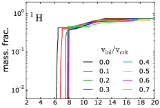
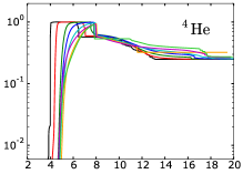
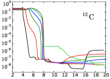
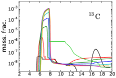
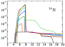
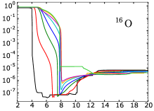
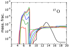
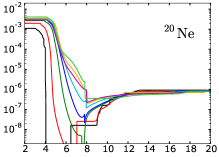
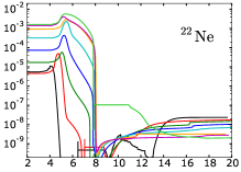
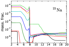
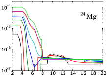
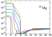
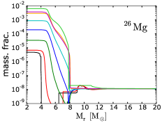
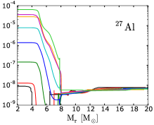
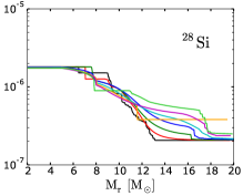
Figure 1: Internal abundance profiles in mass fraction of the 20 $M_{\odot}$ models with various initial rotation rates, at the end of the core He-burning phase.

Table 1: Initial abundances (in mass fraction) of the stellar models. The last line gives the ratio of the initial sum of CNO elements in the models, compared to the Sun.

Isotope	Mass fraction
1H	7.516e-01
3He	4.123-05
4He	2.484e-01
12C	1.292e-06
13C	4.297e-09
14N	1.022e-07
15N	4.024e-10
16O	6.821e-06
17O	3.514e-10
18O	2.001e-09
19F	8.385e-11
20Ne	9.205e-07
21Ne	7.327e-10
22Ne	2.354e-08
23Na	4.135e-09
24Mg	2.012e-07
25Mg	1.030e-08
26Mg	1.179e-08
27Al	7.694e-09
28Si	2.060e-07
(C+N+O) / (C+N+O)⊙	9.444e-04

Table 2: Properties of the 20 $M_{\odot}$ source star models: model label (column 1), $\upsilon_{\text{ini}}/\upsilon_{\text{crit}}$ (column 2), $\Omega_{\text{ini}}/\Omega_{\text{crit}}$ (column 3), initial equatorial velocity (column 4), mean equatorial velocity during the MS (column 5), total lifetime (column 6), mass of the model at the end of the evolution (column $7$).

Model	$\upsilon_{\text{ini}}/\upsilon_{\text{crit}}$	$\Omega_{\text{ini}}/\Omega_{\text{crit}}$	$\upsilon_{\text{ini}}$	$\langle\upsilon_{\text{eq}}\rangle_{\rm MS}$	$\tau_{\text{tot}}$	$M_{\text{fin}}$
			[km/s]	[km/s]	[Myr]	[$M_{\odot}$]
vv0	0.0	0	0	0	8.94	19.998
vv1	0.1	0.15	88	70	9.43	19.998
vv2	0.2	0.32	188	146	9.81	19.960
vv3	0.3	0.46	276	223	10.07	19.726
vv4	0.4	0.69	364	302	10.29	19.625
vv5	0.5	0.71	454	384	10.49	19.189
vv6	0.6	0.81	547	470	10.65	19.222
vv7	0.7	0.90	644	543	11.04	19.764

2.3 Mixing and nucleosynthesis

During the core H-burning and He-burning phase, the mixing induced by rotation changes the distribution of the chemical elements inside the star. In advanced stages (core C-burning and after), the burning timescale becomes small compared to the rotational mixing timescale so that rotation barely affects the distribution of chemical elements. During the core He-burning phase, the rotational mixing triggers exchanges of material between the convective He-burning core and the convective H-burning shell (Maeder & Meynet 2015; Frischknecht et al. 2016; Choplin et al. 2016). In addition, the growing convective He-burning core progressively engulfs the products of H-burning. The main steps of this mixing process are summarized below:

1. In the He-burning core, ¹²C and ¹⁶O are synthesized via the 3$\alpha$ process and ¹²C($\alpha,\gamma$)¹⁶O.

2. The abundant ¹²C and ¹⁶O in the He-burning core are progressively mixed into the H-burning shell. It boosts the CNO cycle and creates primary CNO elements, especially ¹⁴N and ¹³C.

3. The products of the H-burning shell (among them primary ¹³C and ¹⁴N) are mixed back into the He-core. From the primary ¹⁴N, the reaction chain ¹⁴N($\alpha,\gamma$)¹⁸F($e^{+}\nu_{e}$)¹⁸O($\alpha,\gamma$)²²Ne allows the synthesis of primary ²²Ne. The reactions ²²Ne($\alpha,n$) and ²²Ne($\alpha,\gamma$) make ²⁵Mg and ²⁶Mg, respectively. The neutrons released by the ²²Ne($\alpha,n$) reaction produce ¹⁹F, ²³Na, ²⁴Mg, and ²⁷Al by ¹⁴N($n,\gamma$)¹⁵N($\alpha,\gamma$)¹⁹F, ²²Ne($n,\gamma$)²³Ne($e^{-}\bar{\nu}_{e}$)²³Na, ²³Na($n,\gamma$)²⁴Na($e^{-}\bar{\nu}_{e}$)²⁴Mg, and ²⁶Mg($n,\gamma$)²⁷Mg($e^{-}\bar{\nu}_{e}$)²⁷Al, respectively. Free neutrons can also trigger the s-process, provided enough seeds, like ⁵⁶Fe, are present (Pignatari et al. 2008; Frischknecht et al. 2016; Choplin et al. 2018).

4. The newly formed elements in the He-burning core can be mixed again into the H-burning shell. It can boost the Ne-Na and Mg-Al cycles: additional Na and Al can be produced.

Figure 1 shows the results of this mixing process in the 20 $M_{\odot}$ models with various initial rotation rates. The chemical profiles are shown at the end of the core He-burning phase. As the initial rotation increases, the chemicals transit more efficiently from one burning region to another because of stronger rotational mixing and the convective He-burning core tends to grow more, which also facilitates the exchanges of chemicals between the two burning regions. For high initial rotation rates, however ($\upsilon_{\rm ini}/\upsilon_{\rm crit}\gtrsim 0.5$), the growing of the He-core is limited by the very active H-burning shell (the high activity is due to the copious amounts of ¹²C and ¹⁶O entering the shell and boosting the CNO cycle). This effect limits the efficiency of the mixing process for high rotation and makes the production of chemicals starting to saturate for $\upsilon_{\rm ini}/\upsilon_{\rm crit}\gtrsim 0.5$ (e.g. the ¹⁴N or ²²Ne profiles in Fig. 1).

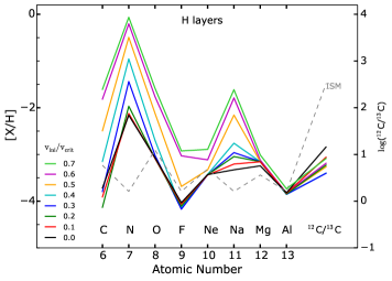
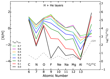
Figure 2: Integrated [X/H] and $\log$(¹²C/¹³C) ratios in the H-rich layers (left panel) and H + He-rich layers (right panel) at the pre-SN stage for the 20 $M_{\odot}$ models with different initial rotation rates. The material ejected through winds during the evolution is included. The dashed line shows the initial source star composition.

While the Ne-Na cycle is boosted in the H-burning shell of rotating models (see the peak of ²³Na at $\sim 8$ $M_{\odot}$), neither the Mg-Al cycle nor the ²⁷Al($p,\gamma$)²⁸Si reaction is significantly boosted (no similar peak in the H-burning shell) because the temperature in the H-burning shell ($T\lesssim 45$ MK) is too low to efficiently activate these reactions. Moreover, the synthesis of extra Al in the H-burning shell needs extra Mg, which is only built in the He-core when $T\gtrsim 220$ MK (through an $\alpha$-capture on ²²Ne). In a 20 $M_{\odot}$ model, this temperature corresponds to the end of the core He-burning phase. The extra Mg created in the core has then little time to be transported to the H-burning shell and boosts the Mg-Al cycle.

2.4 Composition of H- and He-rich layers at the pre-SN stage

H-rich layers

During the evolution of stars, some material is ejected through stellar winds. Rotation is expected to affect the mass loss of massive stars (Maeder 1999; Maeder & Meynet 2000). In these 20 $M_{\odot}$ models, however, losses through winds stay small ($<1$ $M_{\odot}$, see Table 2). The radiative mass loss–metallicity relation ($\dot{M}\propto Z^{0.85}$) plays a major role here and prevents significant radiative mass loss episodes. The left panel of Fig. 2 shows the chemical composition of the H-rich layers at the end of the evolution. It comprises all the material above the bottom of the H-shell (defined where the mass fraction of X(¹H) drops below 0.01). It includes the wind material. Depending on the model, the bottom of the H-shell is located at a mass coordinate in between 6.3 and 8 $M_{\odot}$. The typical CNO pattern appears for all the models (more N, less C and O), but the sum of CNO elements increases with rotation, as a result of ¹²C and ¹⁶O having diffused to the H-burning shell. Thanks to the extra Ne entering in the H-shell and boosting the Ne-Na cycle (see Sect. 2.3), [Na/H] spans $\sim 2$ dex from the non-rotating to the fast rotating model. The [Mg/H] and [Al/H] ratios do not vary more than 0.5 dex. The $\log$(¹²C/¹³C) ratio is close to the CNO equilibrium value of $\sim$ $0.6$.

H-rich and He-rich layers

The right panel of Fig. 2 shows the chemical composition of the H- and He-rich layers. All the material above the bottom of the He-shell (where the mass fraction of X(⁴He) drops below 0.01) is considered. In this case, the mass cuts are between 3.9 and 5.2 $M_{\odot}$, depending on the model. Compared to the previous case, the additional $\sim 2$ $M_{\odot}$ are H-free, so that it raises the [X/H] values slightly (by ¡ 0.5 dex). The CNO pattern is flipped compared to the ejecta of the H-rich layers only because ¹⁴N is depleted, while ¹²C and ¹⁶O are abundant in the region processed by He-burning (Fig. 1). The He-burning products (particularly Ne, Mg, and Al) are boosted compared to the previous case. These products also increase with initial rotation as a result of the back-and-forth mixing process (see Sect. 2.3). In the region processed by He-burning, ¹³C is depleted by ($\alpha,n$) and ($\alpha,\gamma$) reactions so that the ¹²C/¹³C ratio is largely enhanced compared to the case where only the H-rich ejecta is considered. Rotation nevertheless decreases this ratio because of the additional ¹³C that was synthesized in the layers processed by H-burning.

2.5 Effect of the mass cut

Figure 3 shows the effect of varying the mass cut $M_{\rm cut}$ from $\sim 5$ to $\sim 9$ $M_{\odot}$ in the vv4 model. The highest $M_{\rm cut}$ is located in the H-envelope, the lowest value in the He-shell. The numbers in parentheses indicate the mass fraction of ¹H at the mass coordinate equal to the indicated $M_{\rm cut}$. Varying the mass cut from the H- to He-shell flips the CNO pattern. It goes from a $\wedge$-shape to a $\vee$-shape pattern: in the H-shell, the effect of CNO cycle is dominant (high N/C and N/O ratios), while in the He-shell, the C and O produced by He-burning dominate so that the C/N and C/O ratios are dramatically increased. While the $\log$(¹²C/¹³C) is close to the CNO equilibrium value (about $0.6$) for shallow $M_{\rm cut}$, it increases with deeper mass cuts as a results of ¹³C-depletion and ¹²C-richness of the layers processed by He-burning. Deeper mass cuts also increase [Ne/H] or [Na/H] ratios, for instance, as a result of the addition of He-burning material in the ejecta.

3 Linking EMP stars with their source stars

If they were present, the stars discussed in the previous section should have left their chemical imprints on the next stellar generations. We therefore investigate whether the material processed by rotation may be found in the chemical composition of observed EMP stars. For the comparison, the elements C, N, O, Na, Mg, and Al and the ¹²C/¹³C ratio are considered because they are the elements mostly affected by rotation. The possible origin of the heavier elements is discussed in Sect. 5.3.

Table 3: Number of stars in the considered sample (from the SAGA database, Suda et al. 2008, 2017) having a given abundance available (first row) or having only a limit (second row).

	C	N	O	Na	Mg	Al	12C/13C
Abundance	272	75	35	166	271	248	30
Limit	0	54	56	2	0	1	9

3.1 Metal-poor star sample

The stars with $\leq-4$ [Fe/H] $\leq-3$ and with at least three abundance values determined among C, N, O, Na, Mg, Al, and ¹²C/¹³C are selected. This sample comprises 272 stars. The abundance data of the metal-poor stars considered in this work mostly come from the SAGA database (Suda et al. 2008, 2017). The recently observed stars fulfilling the criteria mentioned above were added: G64-12 (Placco et al. 2016a), LAMOSTJ2217+2104 (Aoki et al. 2018), SDSSJ0140+2344, SDSSJ1349+1407 (Bonifacio et al. 2018), SDSSJ0826+6125, SDSSJ1341+4741 (Bandyopadhyay et al. 2018). The individual references are given in Appendix A. Table 3 shows the number of available abundance and limits for the EMP stars considered.

3.2 Internal mixing processes in EMP stars

The link between the EMP star and its source(s) is made more difficult by the fact that EMP stars themselves may have undergone internal mixing processes from their birth (e.g. dredge-up, thermohaline mixing, rotation, or atomic diffusion, Richard et al. 2002; Charbonnel & Zahn 2007; Stancliffe et al. 2009). These processes may have caused surface abundance modifications, so that the abundance of an element derived from observations may be different to the abundance at the birth of the EMP star.

The first dredge-up and the thermohaline mixing, may be the most important processes. They happen in evolved EMP stars and can decrease the C surface abundance and ¹²C/¹³C ratio and increase the N surface abundance (e.g. Charbonnel 1994; Stancliffe et al. 2007; Eggleton et al. 2008; Lagarde et al. 2019). In this work, the evolutionary effects on the surface carbon abundance were corrected following Placco et al. (2014b), who proposed a correction based on stellar models to apply to the carbon abundance of stars with [Fe/H] $<-2$. This correction likely allows the initial surface carbon abundance of metal-poor stars to be recovered. By comparing the Placco et al. (2014b) sample with our sample, we corrected the C abundance of 173 EMP stars. The correction $\Delta$[C/H] applied to the [C/H] ratio varies between 0 and 0.77. After correction, the sample comprises 87 CEMP stars (EMP stars are considered CEMP if [C/Fe] $\geq 0.7$). For N and ¹²C/¹³C, no similar correction is available yet. Here we set the [N/H] and ¹²C/¹³C ratios as upper and lower limits, respectively, for the stars on the upper giant branch ($\log g<2$). These stars may indeed have experienced important modification of their surface N abundance and ¹²C/¹³C ratio. This assumption, and more generally internal mixing processes in EMP stars, is discussed further in Sect. 4.3.3.

We note that most of the CEMP stars considered here belong to group II (Yoon et al. 2016) because the metallicity range considered ($-4<$ [Fe/H] $<-3$) contains mainly group II stars. Group III stars are found at [Fe/H] $\lesssim-4,$ and group I mostly at [Fe/H] $\gtrsim-3$ (their figure 1). In our sample, $\sim 8\%$ of the considered CEMP stars have $A(C)>7$, where group I stars are found.

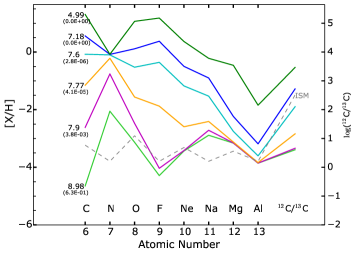
Figure 3: Effect of the mass cut for the vv4 model. The mass cut (in $M_{\odot}$) of the corresponding abundance pattern is indicated on the left. The numbers in parenthesis indicate the ¹H mass fraction in the star at the mass coordinate equal to the mass cut.

3.3 Fitting procedure

To fit the abundances of EMP stars with massive star models, we followed the same procedure described in Heger & Woosley (2010) and Ishigaki et al. (2018), especially for calculating the $\chi^{2}$. Considering N data points, U upper limits, and L lower limits, the $\chi^{2}$ can be computed as

$$\begin{split}\chi^{2}=&\sum^{N}_{i=1}\frac{(D_{i}-M_{i})^{2}}{\sigma^{2}_{o,i}+\sigma^{2}_{t,i}}\\ &+\sum^{N+U}_{i=N+1}\frac{(D_{i}-M_{i})^{2}}{\sigma^{2}_{o,i}+\sigma^{2}_{t,i}}\Theta(M_{i}-D_{i})\\ &+\sum^{N+U+L}_{i=N+U+1}\frac{(D_{i}-M_{i})^{2}}{\sigma^{2}_{o,i}+\sigma^{2}_{t,i}}\Theta(D_{i}-M_{i})\end{split},$$ (1)

where $D_{i}$ and $M_{i}$ are the [X/H] and $\log$(¹²C/¹³C) ratios derived from observations and predicted by source star models, respectively; $\Theta(x)$ is the Heaviside function; and $\sigma_{o,i}$ and $\sigma_{t,i}$ are the observational and theoretical uncertainties. When not available, $\sigma_{o,i}$ is set to $\bar{\sigma}_{o,i}$, which is the mean uncertainty of the sample for the abundance $i$. Mean uncertainties are 0.18, 0.26, 0.17, 0.12, 0.14, and 0.18 dex for [C/H], [N/H], [O/H], [Na/H], [Mg/H], and [Al/H], respectively. The theoretical uncertainties $\sigma_{t,i}$ are set to 0.15 for [C/H], [N/H], and [O/H] and 0.3 for [Na/H], [Mg/H], and [Al/H]. Larger uncertainties for Na, Mg, and Al are considered because of the larger uncertainties on the yields of these elements. The nuclear reaction rates important for the Ne-Na and Mg-Al cycles still suffer significant uncertainties that can affect stellar yields (Decressin et al. 2007; Choplin et al. 2016). The uncertainties associated with ($\alpha$,$\gamma$) or ($\alpha$,$n$) reactions operating in He-burning zones, such as ²²Ne($\alpha$,$\gamma$) or ²²Ne($\alpha$,$n$), are also non-negligible (e.g. Frischknecht et al. 2012). For $\log$(¹²C/¹³C), we set a general sigma value of 0.3 including uncertainties of models and of observations. Theoretical uncertainties are further discussed in Sect. 4.3.2.

For each EMP star, the minimum $\chi^{2}$ is searched among the eight source star models. For each model the mass cut $M_{\rm cut}$ and mass of the added interstellar medium (ISM) $M_{\rm ISM}$ are left as free parameters. The $M_{\rm cut}$ parameter is varied between the bottom of the He-shell (located at $\sim 4-5$ $M_{\odot}$ depending on the model) and the stellar surface, and $M_{\rm ISM}$ is varied between $10^{2}$ and $10^{6}$ $M_{\odot}$. By adding ISM material, we assume some dilution of the source star ejecta with the surrounding ISM. It should occur at the time of the source star explosion. The added ISM material has the same composition as the initial source star composition (dashed line in Figs. 2 and 3). The initial ISM composition and its possible impact on our results are further discussed in Sect. 4.1.2.

3.4 Weighting the source star models

As we show in the next section, it happens that for a given EMP star, more than one of the eight 20 $M_{\odot}$ source star models can give a reasonable solution. To account for this when deriving, for instance, the velocity distribution of the best source star models, we associate a weight with each fit, scaling with the goodness of fit. The goodness of fit is determined thanks to the p-value $p$, which is directly equal to the weight and can be written as

$$p(\chi^{2},N-m)=1-F(\chi^{2},N-m)=1-\frac{\gamma(\frac{N-m}{2},\frac{\chi^{2}}{2})}{\Gamma(\frac{N-m}{2})},$$ (2)

with $F$ the $\chi^{2}$ cumulative distribution function, $\Gamma$ the gamma function, and $\gamma$ the lower incomplete gamma function. Here $N$ is the number of measured abundances for the considered EMP star and $m=2$ is the number of free parameters for a given 20 $M_{\odot}$ model ($M_{\rm cut}$ and $M_{\rm ISM}$). From $\chi^{2}$, $N$, and $m$, the reduced $\chi^{2}$ can be calculated as $\chi_{\nu}^{2}=\chi^{2}/(N-m)$.

Since high $\chi^{2}$ values give negligible weights, the models that give bad fits are automatically discarded and will not contribute to determining the overall characteristics of the best progenitors (e.g. velocity distribution). Similarly, if no good fit can be found for a given EMP star, this EMP star is not considered because of the negligible weights of all the source star models.

We note that the weights for given EMP stars are not normalized to one. If so, the EMP stars that cannot be fitted correctly (hence having low weights for all source star models) will contribute similarly to the well fitted EMP stars. However, it is possible to normalize the weights to one if a threshold $\chi_{\nu,\text{th}}^{2}$ is first set (e.g. $\chi_{\nu,\text{th}}^{2}=3$) so as to discard the EMP stars where no $\chi_{\nu}^{2}<\chi_{\nu,\text{th}}^{2}$ can be found. We checked that this alternative method gives results that are similar to those of the adopted method; the results are presented in the next section.

4 Results

Figure 4 shows the distribution of $\chi^{2}$ of the best model for the 272 star fitted. Two stars with very high $\chi^{2}$ (BS16929-005 and SDSSJ0826+6125 with $\chi^{2}=31$ and 58, respectively) are not shown in Fig. 4. The stars that cannot be fitted correctly are discussed further in Sect. 4.4. Tables 4 and 5 give the fraction of fits having a $\chi^{2}$ and $\chi_{\nu}^{2}$ value below a given threshold, respectively. From Table 4 we see that 60 % (39 %) of the stars have $\chi^{2}<5$ ($\chi^{2}<3$). The CEMP stars show overall better fits than C-normal EMP stars. We also note that the 8 % of CEMP stars with A(C) ¿ 7 (or group I CEMP stars, Yoon et al. 2016) follow a $\chi^{2}$ distribution that is similar to that of the entire CEMP sample. In particular, $61$ % of them have $\chi^{2}<3$.

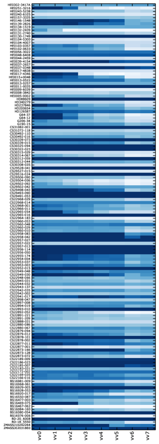
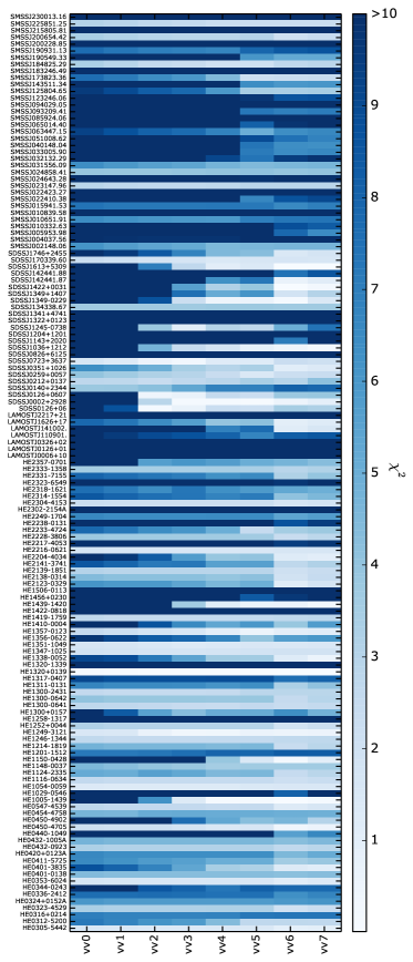
Figure 14: Summary plot of the abundance fitting of the 272 EMP stars with the eight source star models. For a given EMP star (y-axis label) and a given source star model (x-axis label), the colour indicates the best $\chi^{2}$ found.

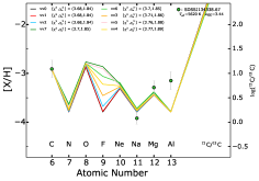
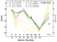
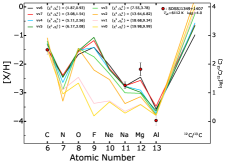
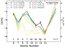
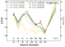
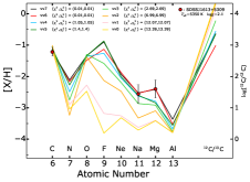
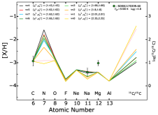
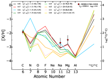
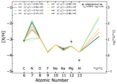
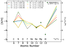
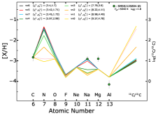
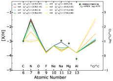
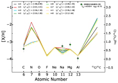
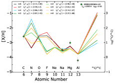
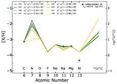
Figure 21: Continued.

Figure 14 in Appendix B shows a summary plot of the abundance fitting of each of the 272 EMP stars considering each of the eight source star models. Figure 21 in Appendix B shows the abundance fitting of all the EMP stars having at least one source star model with $\chi_{\nu}^{2}<2$. Figure 5 shows the abundance fitting of several EMP stars with $\chi^{2}_{\nu}<2$. We discuss below some of these fits individually.

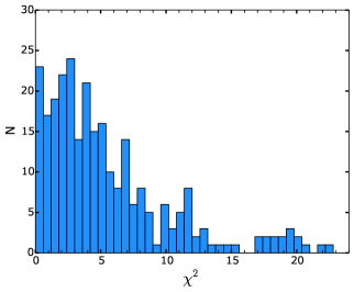
Figure 4: Distribution of the $\chi^{2}$ values for the 272 EMP stars fitted.

HE1439-1420

This star is shown in the top left panel. The C and N abundances of HE1439-1420 are compatible with a $\vee$-shape CNO pattern, but not with a $\wedge$-shape one. As shown in Figs. 2 and 3, $\vee$-shape CNO patterns are characteristics of mass cuts located in the He-shell region. In addition, the high Na and Mg enhancement of this star are best explained by fast rotating models that have experienced significant mixing between the H- and He-burning regions. The best fit is given by the vv7 model, with $M_{\rm cut}=5.45$ $M_{\odot}$ and $M_{\rm ISM}=1789$ $M_{\odot}$. The $\chi^{2}$ map for the vv7 model is shown in Fig. 6. The only minimum $\chi^{2}$ is located at the values mentioned previously. In general, it has been checked for the other EMP stars that only one minimum can be found in the $M_{\rm cut}$ $-$ $M_{\rm ISM}$ plane.

Table 4: Fraction of stars with a $\chi^{2}$ value below a given threshold. Results are given for the entire sample (272 stars), for CEMP stars (87 stars) and for C-normal EMP stars (185 stars).

	$\chi^{2}<10$	$\chi^{2}<5$	$\chi^{2}<3$	$\chi^{2}<2$	$\chi^{2}<1$
All stars	84 %	60 %	39 %	25 %	11 %
CEMP	89 %	77 %	59 %	48 %	30 %
C-normal EMP	82 %	52 %	29 %	14 %	3 %

Table 5: Fraction of fits having a $\chi_{\nu}^{2}$ value (reduced $\chi^{2}$, see text) below a given threshold. Results are given for the entire sample (272 stars), for CEMP stars (87 stars) and for C-normal EMP stars (185 stars).

	$\chi_{\nu}^{2}<10$	$\chi_{\nu}^{2}<5$	$\chi_{\nu}^{2}<3$	$\chi_{\nu}^{2}<2$	$\chi_{\nu}^{2}<1$
All stars	97 %	81 %	58 %	39 %	17 %
CEMP	99 %	91 %	77 %	64 %	40 %
C-normal EMP	96 %	76 %	49 %	26 %	5 %

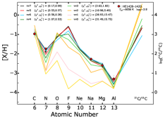
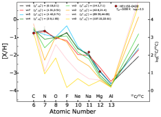
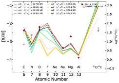
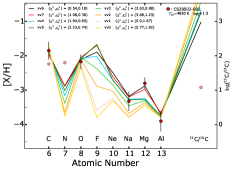
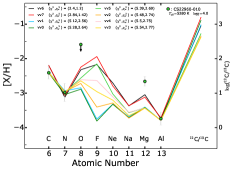
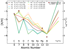
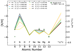
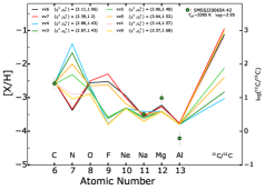
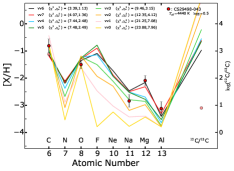
Figure 5: Examples of EMP stars having at least one source star model with $\chi^{2}_{\nu}<2$ ($\chi^{2}\lesssim 3$). Red and green circles denote CEMP ([C/Fe] $>0.7$) and C-normal EMP stars, respectively. For each EMP star, the best fit for each of the 20 $M_{\odot}$ models is shown, ranked by increasing $\chi^{2}$. For evolved EMP stars ($\log g<2$), [N/H] and $\log$(¹²C¹³C) are shown as light red and green symbols and are considered upper and lower limits, respectively. When available, the correction on the C abundance from Placco et al. (2014b) is taken into account. In this case, the [C/H] ratio before (after) correction is shown by a light (normal) red or green symbol. When available, the observational uncertainty is shown by a black bar. If it is not available, the mean observational uncertainty of the EMP sample (Sect. 3.3) is shown as a grey bar.

HE1150-0428

This star is shown in the top middle panel. The best fit is given by the vv6 model, with $M_{\rm cut}=7.46$ $M_{\odot}$ and $M_{\rm ISM}=100$ $M_{\odot}$. This $M_{\rm cut}$ is $\sim 0.4$ $M_{\odot}$ below the bottom of the hydrogen envelope. A deeper $M_{\rm cut}$ will give a more $\vee-$shape pattern for CNO, while a shallower $M_{\rm cut}$ will give a more $\wedge$-shape pattern. HE1150-0428, having [C/H] $\sim$ [N/H] therefore requires a $M_{\rm cut}$ around the bottom of the H-envelope, which is the region where the CNO pattern is flipping from a $\wedge$-shape to a $\vee$-shape.

BD-18_5550

The high [Mg/H] of this star (top right panel) requires both fast rotation and a deep mass cut. The best model is vv6, with $M_{\rm cut}=4.74$ and $M_{\rm ISM}=50941$ $M_{\odot}$.

CS29502-092

This star (shown in the middle left panel) is evolved, with $\log g<2$. Consequently, the [N/H] and ¹²C/¹³C are set as upper and lower limits respectively (see Sect. 3.2). In this case, the good source star models have similar characteristics to those in the previous case (BD-18_5550). The hypothesis of non-efficient internal mixing processes in EMP stars, which means that the [N/H] and ¹²C/¹³C ratios should not be set as limits in evolved stars, is investigated in Sect. 4.3.3.

4.1 Characteristics of the best source star models

We now derive the $M_{\rm cut}$, $M_{\rm ISM}$, and velocity distribution of the best source star models. The following analysis determines the ability of the eight models to fit the entire EMP star sample. Our approach may be seen as statistical: for a given EMP star and source star, the weight attributed to the fit (Sect. 3.4) can be seen as the likelihood of this source star being the true source of this specific EMP star.

In the case of HE1439-1420, the weights associated with the $\chi^{2}$ and $\chi_{\nu}^{2}$ values shown in the top left panel of Fig. 5 are as follows:

• 0.92 for the vv7 model, ($\chi^{2}$, $\chi_{\nu}^{2}$) $=(0.17,0.09)$;

• 0.77 for the vv5 model, ($\chi^{2}$, $\chi_{\nu}^{2}$) $=(0.53,0.27)$;

• 0.76 for the vv6 model, ($\chi^{2}$, $\chi_{\nu}^{2}$) $=(0.56,0.28)$;

• 0.59 for the vv4 model, ($\chi^{2}$, $\chi_{\nu}^{2}$) $=(1.07,0.53)$;

• 0.16 for the vv3 model, ($\chi^{2}$, $\chi_{\nu}^{2}$) $=(3.63,1.82)$;

• $4.2\times 10^{-3}$ for the vv2 model, ($\chi^{2}$, $\chi_{\nu}^{2}$) $=(10.98,5.49)$;

• $1.4\times 10^{-6}$ for the vv1 model, ($\chi^{2}$, $\chi_{\nu}^{2}$) $=(26.93,13.47)$;

• $1.4\times 10^{-7}$ for the vv0 model, ($\chi^{2}$, $\chi_{\nu}^{2}$) $=(31.49,15.75)$.

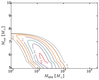
Figure 6: $\chi^{2}$ contour map for the vv7 model, considering the fit of HE1439-1420 (the axis shows the two free parameters $M_{\rm cut}$ and $M_{\rm ISM}$). The numbers associated with the contours give the $\chi^{2}$ values. The minimum $\chi^{2}$ is found for $M_{\rm cut}=5.45$ $M_{\odot}$ and $M_{\rm ISM}=1789$ $M_{\odot}$. These values produce the black pattern shown in the top left panel of Fig. 5.

4.1.1 Mass cut distribution

Figure 7 (top panel) shows the weighted $M_{\rm cut}$ distribution of the source star models. The distribution is normalized to 1. The two peaks in the mass cut distribution correspond to the bottom of the H-shell ($\sim 8$ $M_{\odot}$) and the bottom of the He-burning shell ($\sim 5$ $M_{\odot}$). Around these two mass coordinates, the stellar chemical composition is diverse and therefore a wide variety of chemical patterns, needed to account for the wide variety of EMP star chemical pattern, can be produced. We note that the best solutions for the CEMP stars (red distribution) are preferentially found for deeper $M_{\rm cut}$ in the layers processed by He-burning where C, Na, Mg, and Al are abundant (cf. Figs. 2 and 3).

Finding most of the mass cuts at the bottom of the H-shell and He-shell may be physically motivated by the fact that the energy required to unbind the material above a given mass cut shows jumps at these locations (Fig. 7, middle and bottom panels). By peaking at $\sim 5$ and $\sim 8$ $M_{\odot}$, the derivative of $E_{\rm UB}$ reveals these jumps. The jump at $\sim 8$ $M_{\odot}$ is smaller for slow rotating models (especially vv0 and vv1) because these models do not fully enter the red super giant (RSG) phase (Fig. 8), where the stellar radius expands significantly. On the contrary, since the faster rotating models enter the RSG phase, their envelopes expand dramatically and become loosely bound. Overall, we may expect a clustering of the mass cuts around $\sim 5$ and $\sim 8$ $M_{\odot}$ because the binding energy of most models significantly increases below these mass coordinates, making these deeper layers more difficult to expel.

4.1.2 $M_{\rm ISM}$ distribution

Figure 9 shows the weighted distribution of $M_{\rm ISM}$, the mass of added ISM. The distribution is normalized to 1. The overall blue distribution peaks around low $M_{\rm ISM}$ values. Among the best source star models (with $\chi^{2}<3$), 59 % have $10^{2}<M_{\rm ISM}<10^{3}$ $M_{\odot}$ and 73 % have $10^{2}<M_{\rm ISM}<10^{4}$ $M_{\odot}$. For such $M_{\rm ISM}$ values, the contribution of ISM is generally small compared to the source star contribution. For CEMP stars, it is more equally distributed. It can be understood together with the mass cut distribution: the good solutions for CEMP stars are generally found at deep mass cuts; it therefore requires significant dilution with ISM to not overestimate the CEMP star abundances.

In most cases, even with large $M_{\rm ISM}$, the source star material still dominates. For instance, BD-18_5550 (Fig. 5, top right panel) is best fitted by the vv6 model with ($\chi^{2},\chi^{2}_{\nu}$) = (1.74, 0.87), $M_{\rm cut}=4.74$ $M_{\odot}$, and $M_{\rm ISM}=5.1\times 10^{4}$ $M_{\odot}$. This $M_{\rm ISM}$ value corresponds to $\sim 0.07$ $M_{\odot}$ of carbon. In the source star ejecta there is $\sim 0.59$ $M_{\odot}$ of carbon. Hence, the resulting carbon content reflects more source star material than ISM material. When $M_{\rm cut}\sim 8$ $M_{\odot}$ (i.e. around the second peak, Fig. 7), less carbon is ejected from the source star. The star BS16920-017 is best fit by the vv5 model with ($\chi^{2},\chi^{2}_{\nu}$) = (1.69, 0.84), $M_{\rm cut}=7.99$ $M_{\odot}$ and $M_{\rm ISM}=10^{2}$ $M_{\odot}$. In this case the carbon mass from the stellar ejecta and the ISM are similar, about $10^{-4}$ $M_{\odot}$. However, the total amount of metals is higher in the stellar ejecta ($\sim 3.2\times 10^{-3}$ $M_{\odot}$) compared to the added ISM material ($\sim 9.6\times 10^{-4}$ $M_{\odot}$). This is mainly because there is more nitrogen in the stellar ejecta ($\sim 2.5\times 10^{-3}$ $M_{\odot}$) than in the added ISM ($\sim 10^{-5}$ $M_{\odot}$). The stellar ejecta is enriched in nitrogen because of the operation of the CNO cycle, which was boosted by the progressive arrival of ¹²C and ¹⁶O from the He-burning core.

Generally, apart from the most outer source star layers, the model loses memory of its initial chemical composition as evolution proceeds. The overproduction of C, N, O, Na, Mg, and Al in the source star is mainly due to the primary channel, which means that they were synthesized from the initial H and He content, not the initial metal content. Consequently, and also because the source star material generally dominates over the ISM material, the results should not depend critically on the initial metal mixture considered.

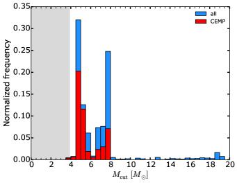
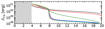
Figure 7: Top panel: Distribution of the source stars $M_{\rm cut}$ values derived from the CEMP star sample (red) and the entire sample (blue). Middle panel : Energy required to unbind the source star material above the considered $M_{\rm cut}$. It is computed as $E_{\rm UB}(M_{\rm cut})=\int_{M_{\rm cut}}^{M_{\rm fin}}GM_{\rm r}/r\leavevmode\nobreak\ \text{d}M_{\rm r}$ with $M_{\rm fin}$ the final source star mass (see Table 2). Bottom panel : Derivative of $E_{\rm UB}$ as a function of $M_{\rm cut}$. The shaded regions show the approximate unexplored $M_{\rm cut}$ region (below the bottom of the He-shell).

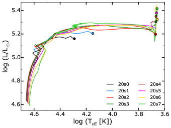
Figure 8: Tracks of the models in the Hertzsprung–Russell diagram. The circles denote the endpoints of the evolution.

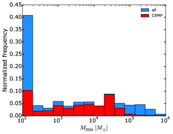
Figure 9: Distribution of the $M_{\rm ISM}$ values derived from the CEMP sample (red) and the entire sample (blue).

4.1.3 Velocity distribution

Figure 10 shows the weighted $\upsilon_{\rm ini}/\upsilon_{\rm crit}$ distribution of the source star models. The distribution is normalized to 1. There is a clear difference between the distribution derived from the C-normal and CEMP stars. For C-normal stars the amount of good fits is comparable, whatever the initial rotation rate. It gives a rather flat $\upsilon_{\rm ini}/\upsilon_{\rm crit}$ distribution; instead, for CEMP stars the ability to find good fits globally increases from non-rotation to fast rotation by a factor of $\sim 6-7$. This difference is due to the fact that C-normal stars generally have low [X/H] ratios, which can often be reproduced by any source star models. It eventually provides similar weights to all the source star models. The CEMP stars are enriched in carbon and also very often in N, O, Na, Mg, and Al, whose production increases with the initial source star rotation. While a large C or O abundance can be achieved in every source star model (Fig. 2, right panel), a large N, Na, Mg or Al abundance is preferentially obtained in fast rotating models. It gives higher weights to rotating models, hence the difference between the red and green distribution in Fig. 10.

The overall $\upsilon_{\rm ini}/\upsilon_{\rm crit}$ distribution follows a trend in between the C-normal EMP and CEMP distributions. The number of good fits increases by a factor of $\sim 3$ from no rotation to fast rotation. For indicative purposes, three fits of the $\upsilon_{\rm ini}/\upsilon_{\rm crit}$ distribution are shown in Fig. 10. The grey fit is of the form $ax+b$, with $(a,b)=(0.192,0.058)$. The blue fit is a fourth-degree polynomial: $\sum_{n=0}^{4}a_{n}x^{n}$ with $(a_{0},a_{1},a_{2},a_{3},a_{4})=(0.064,0.31,-1.71,4.91,-3.90)$. The red fit is the sum of a normal distribution and a skew normal distribution. It is of the form

$$\alpha\leavevmode\nobreak\ g(x;a_{0},b_{0})+\beta\leavevmode\nobreak\ f(x;a_{1},b_{1},c_{1}),$$ (3)

where

$$g(x;a,b)=e^{-(x-a)^{2}/b^{2}}$$ (4)

and

$$f(x;a,b,c)=g(x;a,b)\left[1+erf\left(c\frac{x-a}{b}\right)\right].$$ (5)

The coefficients in Eq. 3 are $(\alpha,\beta,a_{0},b_{0},a_{1},b_{1},c_{1})=(0.14,3.50\times 10^{-2},5.77\times 10^{-1},6.41\times 10^{-1},5.42\times 10^{-1},2.44\times 10^{-1},6.0)$. Although the red fit has the smallest residuals, we cannot exclude the other fits, which also provide reasonable agreements to the distribution.

4.2 Impact on the individual elements on the fitting

In order to check which chemical element(s) can have the largest impact in determining the best EMP source stars, we first inspected two individual stars (CS29498-043 and CS29502-092, shown in Fig. 5) which have all seven abundances determined. We fitted these stars while removing each time one of the seven elements from the fit. Overall, the fits are similar and the ranking of the source star models remains the same, except when removing Mg from the fit. Without Mg, the best fits for these two stars tend to be slower rotators. This shows that Mg may be an important element for constraining the rotation of the EMP source stars.

To check further, we performed the fitting analysis again while removing each time one of the seven elements from the analysis. When removed, an element was not considered to fit any of the EMP stars. Removing either N, O, or ¹²C/¹³C did not affect significantly the distributions shown in Figs. 7, 9, and 10. On the contrary, C and Mg (Na and Al to a smaller extent) mostly determine the shape of the distributions. This is mainly due to the fact that the number of stars with a measured N, O, or ¹²C/¹³C ratio is low compared to the number of stars having a C, Na, Mg, or Al abundance (see Table 3). In addition, some stars with a measured N or ¹²C/¹³C ratio have $\log g<2$ so that only limits were considered (see Sect. 3.2). Also, the observational uncertainties $\sigma_{\rm o}$ for N are on average higher than for C, Na, Mg, and Al (see Sect. 3.3). Overall, it gives less weight to the N abundance compared to other abundances. In the end, C and Mg (Na and Al to a smaller extent) have the highest impact on the derived distributions.

4.3 Robustness of the fitting analysis

4.3.1 Size of the abundance data

The amount of abundance data available varies from one EMP star to another. To check the robustness of our results against the number of abundance constraints, we performed the fitting analysis again by selecting only the EMP stars having at least five measured abundances. While 119 EMP stars have at least five abundances or limits, only 38 have at least five determined abundances. Considering only these 38 stars for the analysis gives a similar increasing trend to that seen in Fig. 10, and a similar double peaked mass cut distribution (Fig. 7). Compared to Fig. 9, the $M_{\rm ISM}$ distribution is more equally distributed between $10^{2}$ and $\sim 10^{5}$ $M_{\odot}$. These overall similar results suggest that the derived distributions are robust against the number of abundance constraints.

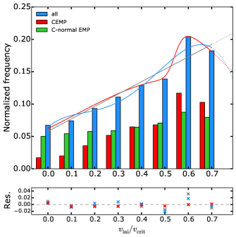
Figure 10: Distribution of the source stars $\upsilon_{\rm ini}/\upsilon_{\rm crit}$ values derived from the CEMP sample (red), the C-normal EMP sample (green), and the entire sample (blue). Three fits of the distribution are shown (red, blue, and grey curves; see text for details) together with their associated residuals (bottom panel).

4.3.2 Varying the theoretical uncertainties

The chemical yields of stellar models depend on processes such as convection, nuclear reaction rates, or the physics of rotation for instance. These processes contain uncertainties that cannot be estimated easily (see also discussion in Sect. 5.5). In this work, the model uncertainties $\sigma_{t,i}$ were treated approximately and set to fixed values (see Sect. 3.3).

As a simple (and limited) approach to investigate the impact of uncertainties on the results, we performed the previous analysis while changing the $\sigma_{t,i}$. We found that increasing the $\sigma_{t,i}$ gives a similar increasing trend for the $\upsilon_{\rm ini}/\upsilon_{\rm crit}$ distribution (Fig. 10), but progressively flattens the distribution. This occurs because with larger uncertainties, the source stars models that had high $\chi^{2}$ values (mostly non-rotating or slow rotating models) now have lower $\chi^{2}$ values and therefore greater weights. It increases the contribution of these models. For instance, setting $\sigma_{t,i}=0.2$ for [C/H], [N/H], and [O/H] (instead of 0.15) and $\sigma_{t,i}=0.4$ for [Na/H], [Mg/H], and [Al/H] (instead of 0.3) gives a contrast (ratio of the highest $\upsilon_{\rm ini}/\upsilon_{\rm crit}$ frequency to the lowest $\upsilon_{\rm ini}/\upsilon_{\rm crit}$ frequency) of 2.3, against 3.0 in the standard case. Increasing $\sigma_{t,i}$ again to 0.25 for C, N, and O and 0.5 for Na, Mg, and Al gives a contrast of 1.9. Overall, the specific slope (or shape) of the $\upsilon_{\rm ini}/\upsilon_{\rm crit}$ depends on the adopted uncertainties, but the dependance likely stays modest.

4.3.3 Internal mixing in EMP stars

Table 6: Same as Table 4, but considering very inefficient internal mixing processes in EMP stars (see text).

	$\chi_{\nu}^{2}<10$	$\chi_{\nu}^{2}<5$	$\chi_{\nu}^{2}<3$	$\chi_{\nu}^{2}<2$	$\chi_{\nu}^{2}<1$
All stars	95 %	77 %	53 %	33 %	14 %
CEMP	98 %	84 %	67 %	57 %	33 %
C-normal EMP	94 %	74 %	46 %	21 %	5 %

The efficiency of the internal mixing processes in low mass stars is still discussed, particularly thermohaline mixing (e.g. Denissenkov & Merryfield 2011; Traxler et al. 2011; Wachlin et al. 2014; Sengupta & Garaud 2018). If these processes were very efficient in EMP stars, we should see a clear separation between the C, N, and ¹²C/¹³C abundances of evolved and unevolved EMP stars, but this is not the case (Choplin et al. 2017a). As a test, we did the analysis again, assuming inefficient internal mixing processes in EMP stars (i.e. their C, N, and ¹²C/¹³C abundances did not change since their birth). In this case the carbon correction from Placco et al. (2014b) was not considered and the N abundance and ¹²C/¹³C ratio were not considered as limits if the EMP star was evolved ($\log g<2$). This new analysis slightly decreases the number of good fits (Table 6) because additional constraints were added (in the evolved EMP stars, N and ¹²C/¹³C are now data points and not limits). The $\upsilon_{\rm ini}/\upsilon_{\rm crit}$ distribution is barely affected. The maximum change in the distribution shown in Fig. 10 is about 4 %. This shows that, based on the current understanding on internal mixing processes (mainly dredge-up and thermohaline mixing), the efficiency of these processes, for the current sample of EMP stars, may not impact much the results presented here.

We also carried out the analysis again while considering only the not-so-evolved EMP stars because the abundances of evolved EMP stars suffer additional uncertainties, and thus their inclusion in the analysis may reduce its robustness. Among the 272 EMP stars, we selected the 128 EMP stars having $\log g\geq 2$. The $\upsilon_{\rm ini}/\upsilon_{\rm crit}$, $M_{\rm cut}$ and $M_{\rm ISM}$ distributions were found to be comparable to the distributions derived from the entire sample. In particular, the overall $\upsilon_{\rm ini}/\upsilon_{\rm crit}$ distribution is very similar to that of Fig. 10.

4.4 EMP stars with high $\chi^{2}$

Stars with [Na, Mg, Al / C] $\gtrsim 0$

The shared feature of about $70\leavevmode\nobreak\ \%$ of the EMP stars having a high $\chi^{2}$ is a relatively high [Mg/C] ratio (a high [Na/C] or [Al/C] ratio to a lesser extent), which cannot be achieved with the considered assumptions (see the five first panels of Fig. 11). In the source star models considered here, [Mg/C] $<0$ (Fig. 2), except in the H-rich layers of non-rotating or slow rotating models (e.g. the black pattern in the left panel of Fig. 2), but in this case, the low [C/H] and [Mg/H] ratios generally cannot account for the EMP star abundances. During the advanced stages of evolution and explosion, the most inner stellar layers are enriched in C, O, Na, Mg, Al, and heavier elements until the Fe-group (e.g. Thielemann et al. 1996; Woosley et al. 2002; Nomoto et al. 2006). Higher [Mg/C] ratios could be obtained in deeper source star layers. This EMP star group with high $\chi^{2}$ and high [Mg/C] ratios may indicate the need for a different source star material, likely originating from deeper layers and possibly processed by explosive nucleosynthesis.

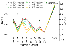
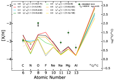
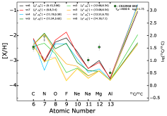
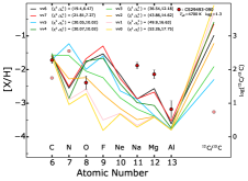
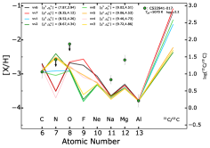
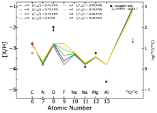
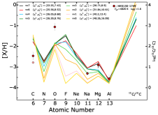
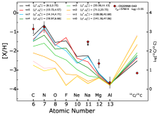
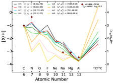
Figure 11: Same as Fig. 5, but for EMP stars with $\chi_{\nu}^{2}>2$ ($\chi^{2}>5$).

Stars with very low [X/H] ratios

Some other EMP stars ($\sim 20$) have at least one very low [X/H] ratio, below the ISM values considered here (e.g. CS22897-008 with a low [Al/H] ratio; see Fig. 11, middle right panel). No solution can give such low values. Zero-metallicity source star models may provide better solutions. A more complete study including source stars spanning a range of different initial metallicities will be addressed in a future work.

Stars with [O/C] $>0$

Several EMP stars ($\sim 5-10$) have very high [O/C] ratios (e.g. HE0130-1749, Fig. 11, bottom left panel). In most of the cases, the source star models predict [O/C] $\leq 0$. Since HE0130-1749 is evolved ($\log g=1.6$), the initial [C/H] was likely higher than the observed value. However, the [O/C] ratio after the Placco et al. (2014a) correction is still well above 0. If the internal mixing processes were much more efficient in HE0130-1749, we might expect a higher [C/H] ratio, which would improve the fit.

Other stars with high $\chi^{2}$

The other problematic EMP stars are generally specific cases. The unevolved star CS22958-042 has a low ¹²C/¹³C (Fig. 11, bottom centre panel) that can only be reproduced in the H-rich layers of source stars (Fig. 2). However, these H-rich layers have [N/C] $\sim 1-2$, while CS22958-042 has [N/C] $\sim 0$. Producing both a low [N/C] with a low ¹²C/¹³C is challenging for these models. A numerical experiment was carried out in Choplin et al. (2017a) in order to try improving the fit for such stars. This peculiar abundance trend can be reproduced if a late mixing event is included in the source star, occurring between the hydrogen- and helium-burning shell, shortly before the end of the source star evolution. In the EMP star sample, only a few stars have a measured C, N, and ¹²C/¹³C ratio together. Moreover, some of these stars are evolved and may have undergone important modifications of these abundances. More N abundances and ¹²C/¹³C ratio measurements in rather unevolved stars are required to further test the idea of a late mixing event in the source star.

Finally, HE1456+0230 (bottom right panel) has a high [C/H], [N/H] together with [N/C] $>0$. This is consistent with material processed by H-burning of a rotating source star. However, in such material, [Na/H] is high, which is not the case for HE1456+0230. Generally, our models predict that a high [N/H] with [N/C] $>0$ should be accompanied with some Na enhancements, together with a low ¹²C/¹³C ratio.

5 Discussions

5.1 CEMP and C-normal EMP stars, and source star matter ejection

While 64 % (40 %) of the CEMP stars have $\chi_{\nu}^{2}<2$ ($\chi_{\nu}^{2}<1$), only 26 % (5 %) of C-normal EMP stars have $\chi_{\nu}^{2}<2$ ($\chi_{\nu}^{2}<1$, Table 5). This important difference between CEMP and C-normal EMP stars suggests that the assumptions made in this study are adequate for most of the CEMP stars, but are not suitable for a large fraction of C-normal EMP stars. In particular, it is likely that the assumption of an explosion with strong fallback (Sect. 2.2) plays a major role and is more suitable for CEMP than C-normal EMP stars. Different kinds of SNe (e.g. more standard core collapse SNe), that could also have existed in the early Universe, may be predominantly responsible for the abundances of C-normal EMP stars. On the contrary, the great fraction of CEMP stars can be explained by source stars that experienced an explosion with strong fallback. We note that the idea of strong fallback was already associated with CEMP stars based on the fact that they have high [C/Fe] ratios and that, in the massive source star, C is located in shallower layers than Fe (e.g. Umeda & Nomoto 2003). Similar conclusions are derived here without considering Fe abundances.

5.2 Comparison with the velocity of nearby OB stars

5.2.1 $\langle\upsilon_{\rm eq}\rangle_{\rm MS}$ distributions

It is worth comparing the derived velocity distribution (Fig. 10) to distributions based on the observation of solar or near-solar metallicity massive stars. Figure 12 shows the distribution of $\langle\upsilon_{\rm eq}\rangle_{\rm MS}$, the mean velocity during the main sequence (MS), for our source star models (the $\langle\upsilon_{\rm eq}\rangle_{\rm MS}$ values are reported in Table 2). These values are representative of $\upsilon_{\rm eq}$ at any stage of the MS because of the modest variation of $\upsilon_{\rm eq}$ during the MS. This is shown by the grey segment at the top of Fig. 12 that represents the $\upsilon_{\rm eq}$ range during the MS for the vv6 model. The three fits in Fig. 12 are the same as in Fig. 10 (see Sect. 4.1.3 for details), but adapted to the new x-axis. The parameters are now $(a,b)=(2.46\times 10^{-4},5.94\times 10^{-2})$ for the grey fit; $(a_{0},a_{1},a_{2},a_{3},a_{4})=(6.40\times 10^{-2},4.14\times 10^{-4},-2.84\times 10^{-6},1.02\times 10^{-8},-1.04\times 10^{-11})$ for the blue fit; and $(\alpha,\beta,a_{0},b_{0},a_{1},b_{1},c_{1})=(0.14,3.5\times 10^{-2},4.5\times 10^{2},5.0\times 10^{2},4.2\times 10^{2},1.8\times 10^{2},6.0)$ for the red fit.

The dashed distribution labelled H+2006 shows the equatorial velocity distribution reported in Huang & Gies (2006), based on the observation of 496 presumably single OB-type stars observed in 19 different Galactic open clusters. The dashed distribution labelled Ra+2013 shows the distribution reported in Ramírez-Agudelo et al. (2013), based on the observation of 216 presumably single O-type stars observed in the 30 Doradus region of the Large Magellanic Cloud. The OB star samples span a range of spectral types which likely correspond to a range of evolutionary stages during the MS. As a first-order comparison, we consider here that the velocity distributions of these two OB star samples are representative of $\langle\upsilon_{\rm eq}\rangle_{\rm MS}$ (x-axis of Fig. 12). This may be a reasonable assumption since these two OB star samples likely contain objects with masses mostly below $30-40$ $M_{\odot}$ and the surface equatorial velocity of solar metallicity models with $M_{\rm ini}\leavevmode\nobreak\ \lesssim\leavevmode\nobreak\ 32$ $M_{\odot}$ does not vary strongly during the MS (Ekström et al. 2012, especially their Fig. 10). The black segment at the top of Fig. 12 illustrates this by showing the range of $\upsilon_{\rm eq}$ during the MS for a 20 $M_{\odot}$ solar metallicity model computed at $\upsilon_{\rm ini}/\upsilon_{\rm crit}=0.3$.

The H+2006 and Ra+2013 distributions peak at 200 and 100 km s^-1. Whether the distribution derived from EMP stars peaks at $\sim 500$ km s^-1 or would still increase toward higher velocities cannot be determined. In any case, a higher fraction of fast rotators and a flatter distribution can be noticed, compared to the distributions derived from observations. We note that while the comparison is made through $\langle\upsilon_{\rm eq}\rangle_{\rm MS}$, the velocity differences are likely significant because the variations in $\upsilon_{\rm eq}$ during the MS are modest compared to the peak difference (see the two segments at the top of Fig. 12).

5.2.2 Two different metallicity regimes

The H+2006 and Ra+2013 distributions are based on OB stars, which are either in open clusters ($-0.5<$ [Fe/H] $<+0.5$ in most of the cases, e.g. Paunzen et al. 2010; Heiter et al. 2014; Netopil et al. 2016) or in the 30 Doradus region (with metallicity $\sim 0.6\leavevmode\nobreak\ Z_{\odot}$ Lebouteiller et al. 2008). This work investigates a much lower metallicity range, sub-solar by a factor of $10^{3}-10^{4}$. Low metallicity stars are less metal-rich so that they are less opaque and more compact. As a consequence, for a given angular momentum content, they tend rotate faster than solar metallicity stars (e.g. Maeder & Meynet 2001). Figure 13 shows the models of Table 2 (blue curve) together with the same models computed at solar metallicity (red curve). For a given initial angular momentum content $L_{\rm ZAMS}$, $\langle\upsilon_{\rm eq}\rangle_{\rm MS}$ is indeed higher at low metallicity. The increasing fraction of fast rotators at low metallicity is supported by observations of rotating massive stars in different metallicity environments (Maeder et al. 1999; Martayan et al. 2007; Hunter et al. 2008; however, the metallicity regime in these studies is not comparable to the very low metallicity regime investigated here).

Figure 13 also shows that the higher fraction of fast rotators in the distribution derived from EMP stars might not be understood solely as a result of the physics of rotating massive stars. According to the additional solar metallicity models we have computed, the peaks of the distributions of Huang & Gies (2006) and Ramírez-Agudelo et al. (2013) correspond to an initial angular momentum of $\sim 1.5-3\times 10^{52}$ g cm² s^-1 (red circles in Fig. 13). The distribution derived in this work peaks at $\sim 4-5\times 10^{52}$ g cm² s^-1 (blue circles). This might indicate that low metallicity massive stars were born with more angular momentum. It might suggest that the removal of angular momentum during massive star formation was less efficient in the early Universe. This may happen if the magnetic braking during star formation is rather inefficient (Hirano & Bromm 2018).

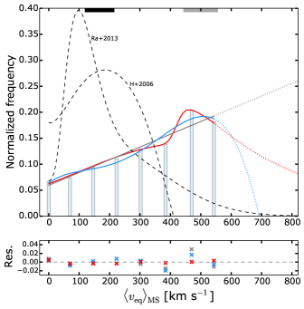
Figure 12: Distribution of the mean equatorial velocity during the MS for the EMP source star models. The three fits are the same as in Fig. 10, but adapted to the new x-axis (see text for details). The dashed black distributions show two equatorial velocity distributions reported in Huang & Gies (2006, H+2006) and Ramírez-Agudelo et al. (2013, Ra+2013), based on the observation of Galactic and LMC O-type and B-type stars (see text for details). The segments at the top show the $\upsilon_{\rm eq}$ range during the MS for the vv6 model (grey) and for a 20 $M_{\odot}$ model computed at solar metallicity with $\upsilon_{\rm ini}/\upsilon_{\rm crit}=0.3$ (black).

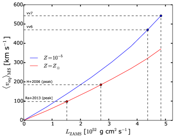
Figure 13: Mean equatorial velocity during the MS as a function of $L_{\rm ZAMS}$, the total angular momentum content at the ZAMS. The two curves show 20 $M_{\odot}$ models computed at solar metallicity (red) and at $Z=10^{-5}$ (blue, the models of Table 2). The two peaks of the Huang & Gies (2006, H+2006) and Ramírez-Agudelo et al. (2013, Ra+2013) velocity distributions are indicated, together with the vv6 and vv7 models.

5.3 Origin of trans-iron elements

Most metal-poor stars having [Fe/H] $<-3$ do not show strong enhancements in trans-iron elements. In our sample, 4 stars have [Sr/Fe] $>1$, 14 have [Ba/Fe] $>1,$ and 7 have [Eu/Fe] $>1$. One possible origin of these elements (or at least some of them) could be due to the s-process operating in the massive source stars, mainly during the core He-burning stage (e.g. Cameron 1960; Peters 1968; Couch et al. 1974; Lamb et al. 1977; Langer et al. 1989; Raiteri et al. 1991). To produce trans-iron elements, this process requires some initial amount of heavy seeds (e.g. Fe) to start with because the neutron flux is too weak to reach trans-iron elements starting from light seeds. Consequently, at zero metallicity, an almost null amount of trans-iron elements is expected. The standard s-process in non-rotating massive stars is likely inefficient below $Z\sim 10^{-4}$ (Prantzos et al. 1990). However, it has been shown that rotation can enhance the neutron flux and therefore boosts the s-process (e.g. Pignatari et al. 2008; Frischknecht et al. 2012; Choplin et al. 2018; Limongi & Chieffi 2018; Banerjee et al. 2019). This can lead to a significant production of trans-iron elements even at low metallicity. In what proportions this process can produce light (e.g. Sr) and heavy (e.g. Pb) trans-iron elements is still uncertain. The inclusion of the s-process in our analysis will be the object of a future work. Other processes or sources may also have contributed to the early enrichment of trans-iron elements, such as AGB stars (e.g. Herwig 2004; Cristallo et al. 2009), jet-like explosions driven by magneto-rotational instabilities (e.g. Winteler et al. 2012; Nishimura et al. 2015), or neutron star mergers (e.g. Thielemann et al. 2017).

5.4 Initial source star masses

The back and forth mixing process likely operates more efficiently in $<60$ $M_{\odot}$ models compared to higher masses models (Choplin et al. 2018), one reason being that higher mass stars have shorter lifetimes hence there is less time for the back and forth mixing process to operate. On the other hand, because higher mass stars have more massive H-shells and He-cores, their mass yields can be higher. Moreover, strong H–He shell interactions can occur in some models and can largely impact the nucleosynthesis (e.g. Ekström et al. 2008). The mass dependency of yields is then complex and it generally varies non-monotonically with initial mass (e.g. Hirschi 2007; Ekström et al. 2008; Yoon et al. 2012; Takahashi et al. 2014). Without a detailed study, it is therefore not possible to predict how our results will depend on the initial source star mass. It is likely, however, that EMP stars with high [Na, Mg, Al/H] ratios may be better reproduced by $\sim 20$ $M_{\odot}$ than $\sim 60$ $M_{\odot}$ models because an overproduction of Na, Mg, or Al requires enough time for the back and forth mixing to operate (Sect. 2.3). The shorter core He-burning stage of higher mass stars may prevent a significant overproduction of Na, Mg, or Al through the back and forth mixing process.

5.5 Rotational mixing uncertainties

Although we investigate the impact of uncertainties in Sect. 4.3.2, we employ a limited approach that cannot fully treat the strong stellar model uncertainties, especially those linked to the rotational mixing. In rotating models, the transport of chemical elements is governed by different diffusion coefficients (e.g. horizontal turbulence or shear mixing). Depending on the prescription used for these coefficients (e.g. Zahn 1992; Mathis et al. 2004; Talon & Zahn 1997; Maeder 1997; Maeder et al. 2013) the production of chemical elements (especially N) can vary significantly (Meynet et al. 2013).

Thanks to asteroseismic observations, it has also been shown that current low mass stellar models likely miss an angular momentum transport process (e.g. Cantiello et al. 2014; Eggenberger et al. 2017). This additional process may also be missing in massive stars. The nature and efficiency of this process is actively discussed (e.g. Eggenberger et al. 2019; Fuller et al. 2019). If added in the present models, it may provide different chemical yields. Brott et al. (2011b) also suggested that an additional mixing process should be included in massive stars to account for the observed population of slow rotating massive stars with high surface nitrogen abundances. The results of this work are subject to important model uncertainties that cannot be fully accounted for with simple approaches, such as the method used in Sect. 4.3.2.

6 Summary and conclusions

In this work, we have investigated whether the peculiar chemical signature of long-dead early massive stars including rotation may be found in the observed extremely metal-poor stars. We computed 20 $M_{\odot}$ models at metallicity $Z=10^{-5}$ with eight initial rotation rates ($0<\upsilon_{\rm ini}/\upsilon_{\rm crit}<0.7$).

The rotational mixing operating between the He-burning core and H-burning shell affects the abundances of light elements from C to Al. At the pre-SN stage, the material above the C-burning shell ($M_{\rm r}\gtrsim 4-5$ $M_{\odot}$) shows a variable chemical composition that strongly depends on the initial rotation. In the H-rich layers, the [C/H], [N/H], [F/H], and [Na/H] ratios are increased by $\sim 1-2$ dex from the non-rotating to the fast rotating case. In the H + He-rich layers, the [N/H], [F/H], [Ne/H], [Na/H], [Mg/H], and [Al/H] ratios are increased by $\sim 2-4$ dex from the non-rotating to the fast rotating case.

We compared the chemical composition of this material with the abundances of EMP stars with $-4<$ [Fe/H] $<-3$. We assumed that the massive stars experienced an explosion with strong fallback. Among the 272 EMP stars considered, $\sim 40-50\leavevmode\nobreak\ \%$ were found to have an abundance pattern consistent with our massive source star models. About $60-70\leavevmode\nobreak\ \%$ ($20-30\leavevmode\nobreak\ \%$) of the CEMP (C-normal EMP) stars can be reasonably well reproduced. In addition, while the abundance patterns of C-normal stars are roughly equally well reproduced by non-rotating and rotating source stars, the patterns of CEMP stars are better explained by fast rotators.

The velocity distribution of the best source star models reaches a maximum at $\upsilon_{\rm ini}/\upsilon_{\rm crit}=0.6-0.7$ (corresponding to initial equatorial velocities of $\sim 550-640$ km s^-1). Compared to the velocity distributions derived from the observation of nearby OB stars, our distribution is flatter and suggests a greater amount of massive fast rotators in the early Universe. The stellar evolution effects (such as the higher compactness of low metallicity stars) may not be sufficient to explain the observed differences. Our results suggest that the initial angular momentum content of early massive stars might have been higher than for solar metallicity massive stars. The possibly higher fraction of fast rotators at low metallicity may have important consequences for the SN types (and rates) from early massive stars, the integrated light of high redshift galaxies and the contribution of early massive stars to reionization.

Caution when using these results is required because of the limiting assumptions made here, especially the explosions with strong fallback (Sect. 2.2). Our results appear to be particularly sensitive to the Mg source star yield (Sect. 4.2), which could change significantly if considering different kind of explosions. As already suggested in the past (e.g. Meynet et al. 2010; Maeder et al. 2015; Choplin et al. 2017a), the ¹²C/¹³C ratio and N abundance should be among the best elements to probe the mixing process(es) at work in early massive stars. Consequently, more ¹²C/¹³C and N measurements (preferentially in non-evolved EMP stars) are desirable to better probe these processes. Finally, caution is also required because of the strong stellar model uncertainties, particularly on the physics of rotational mixing (Sect. 5.5).

Appendix A

Individual references for the considered stars include Jacobson et al. (2015), Roederer et al. (2014b), Andrievsky et al. (2007), Hollek et al. (2011), Spite et al. (2006), Bonifacio et al. (2007), Bonifacio et al. (2009), Lai et al. (2008), Spite et al. (2005), Cohen et al. (2013), Honda et al. (2004), Lai et al. (2007), Andrievsky et al. (2010), Andrievsky et al. (2008), Cayrel et al. (2004), Honda et al. (2011), Allen et al. (2012), Zhang et al. (2011), Barklem et al. (2005), Roederer et al. (2014a), Roederer et al. (2009), Venn et al. (2004), Aoki et al. (2009), Sbordone et al. (2010), Preston et al. (2006), Masseron et al. (2012), Spite et al. (2014), Aoki et al. (2005), Sivarani et al. (2006), Siqueira Mello et al. (2014), Masseron et al. (2006), Boesgaard et al. (2011), Placco et al. (2016a), Ren et al. (2012), Placco et al. (2014a), Hansen et al. (2015), Hansen et al. (2014), Yong et al. (2013), Aoki et al. (2007), Frebel et al. (2007), Cohen et al. (2006), Li et al. (2015), Li et al. (2015), Matsuno et al. (2017), Aoki et al. (2018), Aoki et al. (2008), Aoki et al. (2013), Bonifacio et al. (2018), Bonifacio et al. (2015), Bandyopadhyay et al. (2018), Matsuno et al. (2017), Behara et al. (2010), Spite et al. (2013), Placco et al. (2015), Aguado et al. (2016), Susmitha Rani et al. (2016), Aoki (2010).

Appendix B

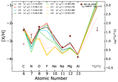
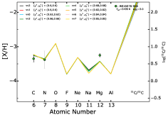
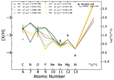
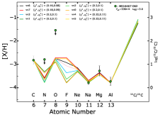
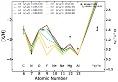
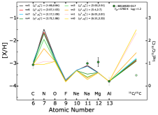
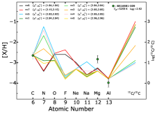
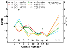
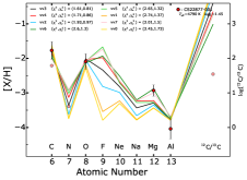
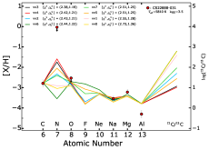
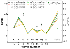
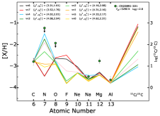
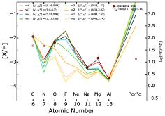
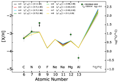
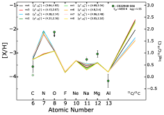
Figure 15: EMP stars having at least one source star model with $\chi_{\nu}^{2}<2$. Red and green circles denote CEMP ([C/Fe] $>0.7$) and C-normal EMP stars, respectively. For evolved EMP stars ($\log g<2$), [N/H] and $\log$(¹²C¹³C) are shown as light red or green symbols and are considered upper and lower limits, respectively. When available, the correction on the C abundance from Placco et al. (2014b) is taken into account. In this case, the [C/H] ratio before (after) correction is shown by a light (normal) red or green symbol. When available, the observational uncertainty is shown by a black bar. If it is not available, the mean observational uncertainty of the EMP sample (Sect. 3.3) is shown as a grey bar.

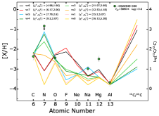
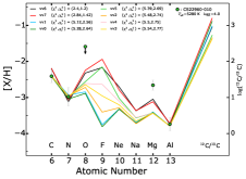
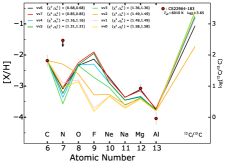
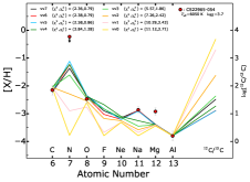
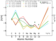
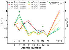
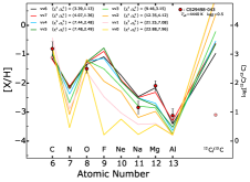
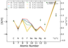
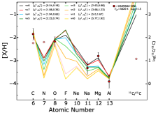
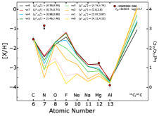
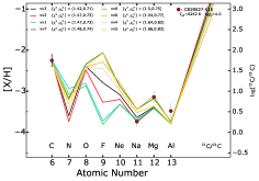
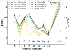
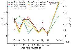
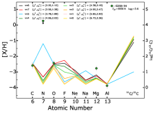
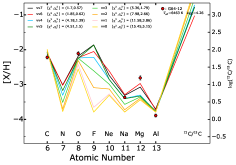
Figure 16: Continued.

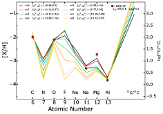
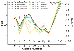
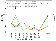
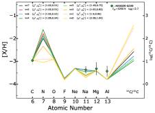
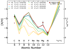
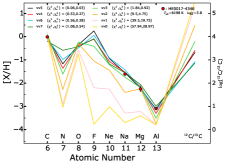
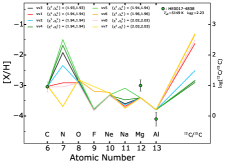
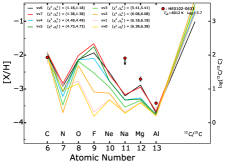
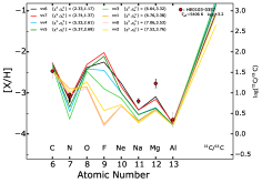
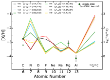
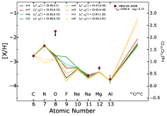
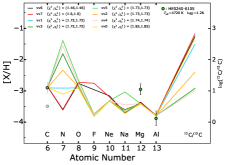
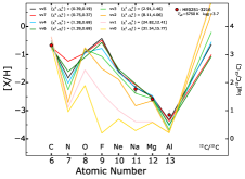
Figure 17: Continued.

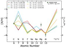
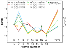
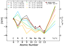
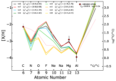
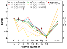
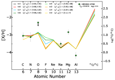
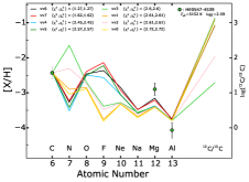
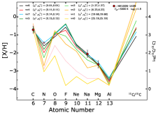
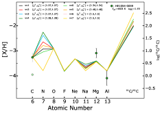
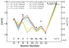
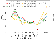
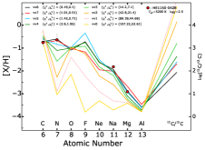
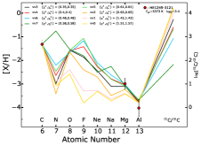
Figure 18: Continued.

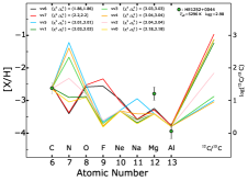
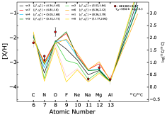
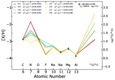
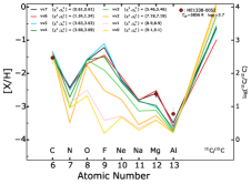
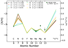
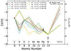
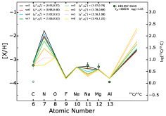
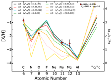
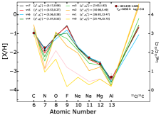
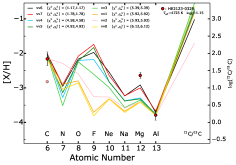
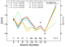
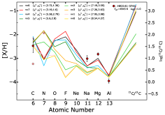
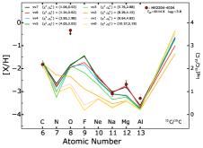
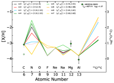
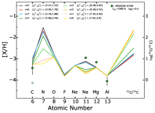
Figure 19: Continued.

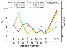
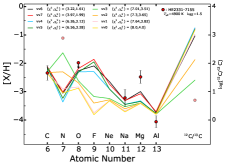
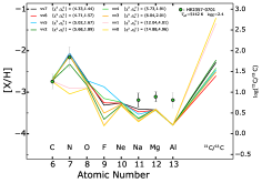
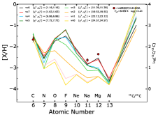
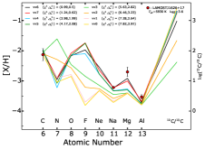
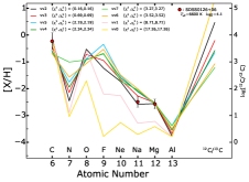
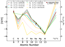
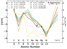
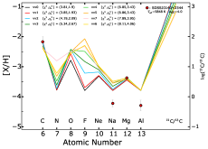
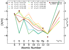
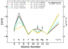
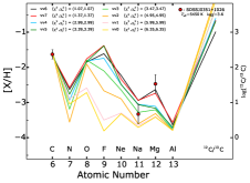
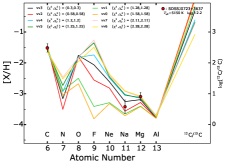
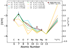
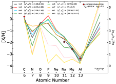
Figure 20: Continued.