Adaptive IGAFEM with optimal convergence rates: T-splines

Abstract.

We consider an adaptive algorithm for finite element methods for the isogeometric analysis (IGAFEM) of elliptic (possibly non-symmetric) second-order partial differential equations. We employ analysis-suitable T-splines of arbitrary odd degree on T-meshes generated by the refinement strategy of [Morgenstern, Peterseim, Comput. Aided Geom. Design 34 (2015)] in 2D and [Morgenstern, SIAM J. Numer. Anal. 54 (2016)] in 3D. Adaptivity is driven by some weighted residual a posteriori error estimator. We prove linear convergence of the error estimator (which is equivalent to the sum of energy error plus data oscillations) with optimal algebraic rates with respect to the number of elements of the underlying mesh.

1. Introduction

1.1. Adaptivity in isogeometric analysis

The central idea of isogeometric analysis (IGA) [HCB05, CHB09, BBdVC⁺06] is to use the same ansatz functions for the discretization of the partial differential equation (PDE) as for the representation of the problem geometry in computer aided design (CAD). While the CAD standard for spline representation in a multivariate setting relies on tensor-product B-splines, several extensions of the B-spline model have emerged to allow for adaptive refinement, e.g., (analysis-suitable) T-splines [SZBN03, DJS10, SLSH12, BdVBSV13], hierarchical splines [VGJS11, GJS12, KVVdZvB14], or LR-splines [DLP13, JKD14]; see also [JRK15, HKMP17] for a comparison of these approaches. All these concepts have been studied via numerical experiments. However, to the best of our knowledge, the thorough mathematical analysis of adaptive isogeometric finite element methods (IGAFEM) is so far restricted to hierarchical splines [BG16, BG17, GHP17, BG18, BBGV19]. Recently, linear convergence at optimal algebraic rate with respect to the number of mesh elements has been proved in [BG17] for the refinement strategy of [BG16] based on truncated hierarchical B-splines [GJS12], and in our own work [GHP17] for a newly proposed refinement strategy based on standard hierarchical B-splines. In the latter work, we identified certain abstract properties for the underlying meshes, the mesh-refinement, and the finite element spaces that imply well-posedness, reliability, and efficiency of a residual a posteriori error estimator and guarantee linear convergence at optimal rate for a related adaptive mesh-refining algorithm. Moreover, in [GHP17] we verified these properties in the case of hierarchical splines. We stress that adaptivity is well understood for standard FEM with globally continuous piecewise polynomials; see, e.g., [Dör96, MNS00, BDD04, Ste07, CKNS08, FFP14, CFPP14] for milestones on convergence and optimal convergence rates. In the frame of adaptive isogeometric boundary element methods (IGABEM), we also mention our recent works [FGP15, FGHP16, FGHP17, Gan17, GPS19a].

1.2. Model problem

On the bounded Lipschitz domain $\Omega\subset{\mathbb{R}}^{d}$, $d\in\{2,3\}$, with initial mesh ${\mathcal{T}}_{0}$ and for given $f\in L^{2}(\Omega)$ as well as $\boldsymbol{f}\in L^{2}(\Omega)^{d}$ with $\boldsymbol{f}|_{T}\in\boldsymbol{H}({\rm div},T)$ for all $T\in{\mathcal{T}}_{0}$, we consider a general second-order linear elliptic PDE in divergence form with homogenous Dirichlet boundary conditions

$$\begin{split}\mathcal{L}u:=-{\rm div}(\textit{{A}}\nabla u)+\textit{{b}}\cdot\nabla u+cu&=f+{\rm div}\boldsymbol{f}\quad\text{in }\Omega,\\ u&=0\quad\text{on }\partial\Omega.\end{split}$$ (1.1)

We pose the following regularity assumptions on the coefficients: $\textit{{A}}(x)\in{\mathbb{R}}^{d\times d}_{\mathrm{sym}}$ is a symmetric and uniformly positive definite matrix with $\textit{{A}}\in L^{\infty}(\Omega)^{d\times d}$ and $\textit{{A}}|_{T}\in W^{1,\infty}(T)$ for all $T\in{\mathcal{T}}_{0}$. The vector $\textit{{b}}(x)\in{\mathbb{R}}^{d}$ and the scalar $c(x)\in{\mathbb{R}}$ satisfy that $\textit{{b}},c\in L^{\infty}(\Omega)$. We interpret $\mathcal{L}$ in its weak form and define the corresponding bilinear form

$$\langle w\,,\,v\rangle_{\mathcal{L}}:=\int_{\Omega}\textit{{A}}(x)\nabla w(x)\cdot\nabla v(x)+\textit{{b}}(x)\cdot\nabla w(x)v(x)+c(x)w(x)v(x)\,dx.$$ (1.2)

The bilinear form is continuous, i.e., it holds that

$$\langle w\,,\,v\rangle_{\mathcal{L}}\leq\big{(}\|\textit{{A}}\|_{L^{\infty}(\Omega)}+\|\textit{{b}}\|_{L^{\infty}(\Omega)}+\|c\|_{L^{\infty}(\Omega)}\big{)}\|w\|_{H^{1}(\Omega)}\|v\|_{H^{1}(\Omega)}\text{ for all $v,w\in H^{1}(\Omega)$.}$$ (1.3)

Additionally, we suppose ellipticity of $\langle\cdot\,,\,\cdot\rangle_{\mathcal{L}}$ on $H^{1}_{0}(\Omega)$, i.e.,

$$\langle v\,,\,v\rangle_{\mathcal{L}}\geq C_{\rm ell}\|v\|_{H^{1}(\Omega)}^{2}\quad\text{for all }v\in H_{0}^{1}(\Omega).$$ (1.4)

Note that (1.4) is for instance satisfied if $\textit{{A}}(x)$ is uniformly positive definite and if $\textit{{b}}\in\boldsymbol{H}({\rm div},\Omega)$ with $-\frac{1}{2}\,{\rm div}\,\textit{{b}}(x)+c(x)\geq 0$ almost everywhere in $\Omega$.

Overall, the boundary value problem (1.1) fits into the setting of the Lax–Milgram theorem and therefore admits a unique solution $u\in H_{0}^{1}(\Omega)$ to the weak formulation

$$\langle u\,,\,v\rangle_{\mathcal{L}}=\int_{\Omega}fv-\boldsymbol{f}\cdot\nabla v\,dx\quad\text{for all }v\in H^{1}_{0}(\Omega).$$ (1.5)

Finally, we note that the additional regularity $\boldsymbol{f}|_{T}\in\boldsymbol{H}({\rm div},T)$ and $\textit{{A}}|_{T}\in W^{1,\infty}(T)$ for all $T\in{\mathcal{T}}_{0}$ is only required for the well-posedness of the residual a posteriori error estimator; see Section 2.5.

1.3. Outline & Contributions

The remainder of this work is organized as follows: Section 2 recalls the definition of T-meshes and T-splines of arbitrary odd degree in the parameter domain (Section 2.1) from [BdVBSV13] for $d=2$ and from [Mor16] for $d=3$. Moreover, it recalls corresponding refinement strategies (Section 2.2) from [MP15, Mor16], derives a canonical basis for the T-spline space with homogeneous boundary conditions (Section 2.3), and transfers all the definitions to the physical domain $\Omega$ via some parametrization $\gamma:[0,1]^{d}\to\overline{\Omega}$ (Section 2.4). Subsequently, we formulate a standard adaptive algorithm (Algorithm 2.7) of the form

$$\boxed{\texttt{solve}}\longrightarrow\boxed{\texttt{estimate}}\longrightarrow\boxed{\texttt{mark}}\longrightarrow\boxed{\texttt{refine}}$$ (1.6)

driven by some residual a posteriori error estimator (2.37). For T-splines in 2D, this algorithm has already been investigated numerically in [HKMP17]. Finally, our main result Theorem 2.11 is presented. First, it states that the error estimator $\eta_{\color[rgb]{0,0,0}}$ associated with the FEM solution $U_{\color[rgb]{0,0,0}}\in{\mathcal{X}}_{\color[rgb]{0,0,0}}\subset H^{1}_{0}(\Omega)$ is efficient and reliable, i.e., there exist $C_{\rm eff}$, $C_{\rm rel}>0$ such that

$$C_{\rm eff}^{-1}\,\eta_{\color[rgb]{0,0,0}}\leq\inf_{V_{\color[rgb]{0,0,0}}\in{\mathcal{X}}_{\color[rgb]{0,0,0}}}\big{(}\|u-V_{\color[rgb]{0,0,0}}\|_{H^{1}(\Omega)}+{\rm osc}_{\color[rgb]{0,0,0}}(V_{\color[rgb]{0,0,0}})\big{)}\leq\|u-U_{\color[rgb]{0,0,0}}\|_{H^{1}(\Omega)}+{\rm osc}_{\color[rgb]{0,0,0}}(U_{\color[rgb]{0,0,0}})\leq C_{\rm rel}\,\eta_{\color[rgb]{0,0,0}},$$ (1.7)

where $\eta_{\ell}$ denotes the error estimator in the $\ell$-th step of the adaptive algorithm and ${\rm osc}_{\color[rgb]{0,0,0}}(\cdot)$ denotes the corresponding data oscillation terms (see (2.41)). Second, it states that Algorithm 2.7 leads to linear convergence with optimal rates in the spirit of [Ste07, CKNS08, CFPP14]: There exist $C>0$ and $0<q<1$ such that

$$\eta_{\ell+j}\leq C\,q^{j}\,\eta_{\ell}\quad\text{for all }\ell,j\in{\mathbb{N}}_{0}.$$ (1.8)

Moreover, for sufficiently small marking parameters in Algorithm 2.7, the estimator (and thus equivalently also the so-called total error $\|u-U_{\ell}\|_{H^{1}(\Omega)}+{\rm osc}_{\ell}(U_{\ell})$; see (1.7)) decays even with the optimal algebraic convergence rate with respect to the number of mesh elements, i.e.,

$$\eta_{\ell}={\mathcal{O}}\big{(}(\#{\mathcal{T}}_{\ell})^{-s}\big{)}\quad\text{for all }\ell\in{\mathbb{N}}_{0},$$ (1.9)

whenever the rate $s>0$ is possible for optimally chosen meshes. The proof of Theorem 2.11 is postponed to Section 3 and is based on abstract properties of the underlying meshes, the mesh-refinement, the finite element spaces, and the oscillations which have been identified in [GHP17] and imply (an abstract version of) Theorem 2.11. In Section 3, we briefly recapitulate these properties and verify them for the present T-spline setting. The final Section 4 comments on possible extensions of Theorem 2.11.

1.4. General notation

Throughout, $|\cdot|$ denotes the absolute value of scalars, the Euclidean norm of vectors in ${\mathbb{R}}^{d}$, and the $d$-dimensional measure of a set in ${\mathbb{R}}^{d}$. Moreover, $\#$ denotes the cardinality of a set as well as the multiplicity of a knot within a given knot vector. We write $A\lesssim B$ to abbreviate $A\leq CB$ with some generic constant $C>0$, which is clear from the context. Moreover, $A\simeq B$ abbreviates $A\lesssim B\lesssim A$. Throughout, mesh-related quantities have the same index, e.g., ${\mathcal{X}}_{\bullet}$ is the ansatz space corresponding to the mesh ${\mathcal{T}}_{\bullet}$. The analogous notation is used for meshes ${\mathcal{T}}_{\circ}$, ${\mathcal{T}}_{\star}$, ${\mathcal{T}}_{\ell}$ etc. Moreover, we use $\widehat{\cdot}$ to transfer quantities in the physical domain $\Omega$ to the parameter domain $\widehat{\Omega}$, e.g., we write $\widehat{\mathbb{T}}$ for the set of all admissible meshes in the parameter domain, while $\mathbb{T}$ denotes the set of all admissible meshes in the physical domain.

2. Adaptivity with T-splines

In this section, we recall the formal definition of T-splines from [BdVBSV13] for $d=2$ and from [Mor16] for $d=3$ as well as corresponding mesh-refinement strategies from [MP15, Mor16]. While the mathematically sound definition is a bit tedious, the basic idea of T-splines is simple: Given a rectangular mesh (with hanging nodes) as in Figure 2.3, one associates to all nodes a local knot vector in each direction as the intersections (projected into the white area $\overline{\widehat{\Omega}}$) of the line in that direction through the node (indicated in red) with the mesh skeleton. The resulting local knot vectors then induce a standard tensor-product B-spline, and the set of all such B-splines spans the corresponding T-spline space. Moreover, we formulate an adaptive algorithm (Algorithm 2.7) for conforming FEM discretizations of our model problem (1.1), where adaptivity is driven by the residual a posteriori error estimator (see (2.37) below). Our main result of the present work Theorem 2.11 states reliability and efficiency of the estimator as well as linear convergence at optimal algebraic rate with respect to the number of mesh elements.

2.1. T-meshes and T-splines in the parameter domain $\mathbb{\widehat{\Omega}}$

Meshes ${\mathcal{T}}_{\bullet}$ and corresponding spaces ${\mathcal{X}}_{\bullet}$ are defined through their counterparts on the parameter domain

$$\widehat{\Omega}:=(0,N_{1})\times\dots\times(0,N_{d}),$$ (2.1)

where $N_{i}\in{\mathbb{N}}$ are fixed integers for $i\in\{1,\dots,d\}$. Recall that the symbol $\bullet$ is used for a generic mesh index to relate corresponding quantities; see the general notation of Section 1.4. Let $p_{1},\dots,p_{d}\geq 3$ be fixed odd polynomial degrees. Let $\widehat{\mathcal{T}}_{0}$ be an initial uniform tensor-mesh of the form

$$\widehat{\mathcal{T}}_{0}=\Big{\{}\prod_{i=1}^{d}[a_{i},a_{i}+1]:a_{i}\in\{0,\dots,N_{i}-1\}\text{ for }i\in\{1,\dots,d\}\Big{\}}.$$ (2.2)

For an arbitrary hyperrectangle $\widehat{T}=[a_{1},b_{1}]\times\dots[a_{d},b_{d}]$, we define its bisection in direction $i\in\{1,\dots,d\}$ as the set

$$\begin{split}{\tt bisect}_{i}(\widehat{T}):=\Big{\{}&\prod_{j=1}^{i-1}[a_{j},b_{j}]\times\Big{[}a_{i},\frac{a_{i}+b_{i}}{2}\Big{]}\times\prod_{j=i+1}^{d}[a_{j},b_{j}],\\ &\prod_{j=1}^{i-1}[a_{j},b_{j}]\times\Big{[}\frac{a_{i}+b_{i}}{2},b_{i}\Big{]}\times\prod_{j=i+1}^{d}[a_{j},b_{j}]\Big{\}}.\end{split}$$ (2.3)

For $k\in{\mathbb{N}}_{0}$, let

$$\underline{k}:=\lfloor k/d\rfloor d$$ (2.4)

and define the $k$-th uniform refinement of $\widehat{\mathcal{T}}_{0}$ inductively by

$$\widehat{\mathcal{T}}_{{\rm uni}(0)}:=\widehat{\mathcal{T}}_{0}\quad\text{and}\quad\widehat{\mathcal{T}}_{{\rm uni}(k)}:=\bigcup\big{\{}{\tt bisect}_{k+1-\underline{k}}(\widehat{T})\,:\,\widehat{T}\in\widehat{\mathcal{T}}_{{\rm uni}(k-1)}\big{\}};$$ (2.5)

see Figure 2.1 and 2.2. Note that the direction of bisection changes periodically.

Figure 2.1. Uniform refinements of 2D initial partition $\widehat{\mathcal{T}}_{0}:=\{[0,1]^{2}\}$.

Figure 2.2. Uniform refinements of 3D initial partition $\widehat{\mathcal{T}}_{0}:=\{[0,1]^{3}\}$.

A finite set $\widehat{\mathcal{T}}_{\bullet}$ is a T-mesh (in the parameter domain), if $\widehat{\mathcal{T}}_{\bullet}\subseteq\bigcup_{k\in{\mathbb{N}}_{0}}\widehat{\mathcal{T}}_{{\rm uni}(k)}$, $\bigcup_{\widehat{T}\in\widehat{\mathcal{T}}_{\bullet}}\widehat{T}=\overline{\widehat{\Omega}}$, and $|\widehat{T}\cap\widehat{T}^{\prime}|=0$ for all $\widehat{T},\widehat{T}^{\prime}\in\widehat{\mathcal{T}}_{\bullet}$ with $\widehat{T}\neq\widehat{T}^{\prime}$. For an illustrative example of a general T-mesh, see Figure 2.3. Since $\widehat{\mathcal{T}}_{{\rm uni}(k)}\cap\widehat{\mathcal{T}}_{{\rm uni}(k^{\prime})}=\emptyset$ for $k,k^{\prime}\in{\mathbb{N}}_{0}$ with $k\neq k^{\prime}$, each element $\widehat{T}\in\widehat{\mathcal{T}}_{\bullet}$ has a natural level

$${\rm level}(\widehat{T}):=k\in{\mathbb{N}}_{0}\quad\text{with }\widehat{T}\in\widehat{\mathcal{T}}_{{\rm uni}(k)}.$$ (2.6)

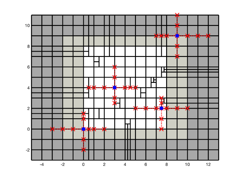
Figure 2.3. A general (non-admissible) T-mesh $\widehat{\mathcal{T}}_{\bullet}^{\rm ext}$ in 2D with $(p_{1},p_{2})=(5,3)$ is depicted. The sets $\widehat{\Omega}$, $\widehat{\Omega}^{\rm act}$, and $\widehat{\Omega}^{\rm ext}$ are highlighted in white, light gray, and dark gray, respectively. For the three (blue) nodes $z\in\{(0,0),(3,4),{\color[rgb]{0,0,0}},(9,9)\}$, their corresponding local index vectors $\widehat{\mathcal{I}}_{\bullet,i}^{\rm loc}(z)$ with $i\in\{1,2\}$ are indicated by (red) crosses. We also indicate in red the lines through the nodes mentioned at the beginning of Section 2. The local knot vectors are obtained by setting all negative values to $0$ and all values larger than $8$ to $8$, i.e., $\widehat{\mathcal{K}}_{\bullet,1}^{\rm loc}\big{(}(0,0)\big{)}=(0,0,0,0,0.5,1,2)$, $\widehat{\mathcal{K}}_{\bullet,2}^{\rm loc}\big{(}(0,0)\big{)}=(0,0,0,1,1.5)$, $\widehat{\mathcal{K}}_{\bullet,1}^{\rm loc}\big{(}(3,4)\big{)}=(0.5,1,2,3,4,4.5,5)$, $\widehat{\mathcal{K}}_{\bullet,2}^{\rm loc}\big{(}(3,4)\big{)}=(2.5,3,4,5,6)$, $\widehat{\mathcal{K}}_{\bullet,1}^{\rm loc}\big{(}(7.5,2)\big{)}=(5,6,7,7.5,8,8,8)$, $\widehat{\mathcal{K}}_{\bullet,2}^{\rm loc}\big{(}(7.5,2)\big{)}=(0,1,2,2.5,3)$, $\widehat{\mathcal{K}}_{\bullet,1}^{\rm loc}\big{(}(9,9)\big{)}=(7,7.5,8,8,8,8,8)$, $\widehat{\mathcal{K}}_{\bullet,2}^{\rm loc}\big{(}(9,9)\big{)}=(7,8,8,8,8)$. This guarantees that all associated B-splines have support within the closure of $\widehat{\Omega}$.

In order to define T-splines, in particular to allow for knot multiplicities larger than one at the boundary, we have to extend the mesh $\widehat{\mathcal{T}}_{\bullet}$ on $\overline{\widehat{\Omega}}$ to a mesh on $\overline{\widehat{\Omega}^{\rm ext}}$, where

$$\widehat{\Omega}^{\rm ext}:=\prod_{i=1}^{d}(-p_{i},N_{i}+p_{i}).$$ (2.7)

We define $\widehat{\mathcal{T}}_{0}^{\rm ext}$ analogously to (2.2) and $\widehat{\mathcal{T}}_{\bullet}^{\rm ext}$ as the mesh on $\overline{\widehat{\Omega}^{\rm ext}}$ that is obtained by extending any bisection, which takes place on the boundary $\partial\widehat{\Omega}$ during the refinement from $\widehat{\mathcal{T}}_{0}$ to $\widehat{\mathcal{T}}_{\bullet}$, to the set $\overline{\widehat{\Omega}^{\rm ext}}\setminus\overline{\widehat{\Omega}}$; see Figure 2.3. For $d=2$, this formally reads

$$\widehat{\mathcal{T}}_{\bullet}^{\rm ext}:=\widehat{\mathcal{T}}_{\bullet}\cup\big{\{}{\rm ext}_{\bullet}(\widehat{E}_{1}\times\widehat{E}_{2})\,:\,{\rm dim}(\widehat{E}_{1}\times\widehat{E}_{2})<2\wedge\widehat{E}_{i}\in\{\{0\},\{N_{i}\},[0,N_{i}]\}\text{ for }i\in\{1,2\}\big{\}},$$ (2.8)

where

$${\rm ext}_{\bullet}\big{(}\{(0,0)\}\big{)} :=\big{\{}[a_{1},a_{1}+1]\times[a_{2},a_{2}+1]\,:\,a_{i}\in\{-p_{i},\dots,-1\}\text{ for }i\in\{1,2\}\big{\}},$$

$${\rm ext}_{\bullet}\big{(}[0,N_{1}]\times\{0\})\big{)} :=\big{\{}[a_{1},b_{1}]\times[a_{2},a_{2}+1]\,:\,a_{2}\in\{-p_{2},\dots,-1\}\wedge\exists b_{2}^{\prime}:[a_{1},b_{1}]\times[0,b_{2}^{\prime}]\in\widehat{\mathcal{T}}_{\bullet}\big{\}},$$

and the remaining ${\rm ext}_{\bullet}(\cdot)$ terms are defined analogously. Note that the logical expression

$$\exists b_{2}^{\prime}:[a_{1},b_{1}]\times[0,b_{2}^{\prime}]\in\widehat{\mathcal{T}}_{\bullet}$$

means that there exists an element at the (lower part of the) boundary $\partial\widehat{\Omega}$ with side $[a_{1},b_{1}]$. For $d=3$, this reads

$$\widehat{\mathcal{T}}_{\bullet}^{\rm ext}:=\widehat{\mathcal{T}}_{\bullet}\cup\Big{\{}{\rm ext}_{\bullet}\Big{(}{\prod_{i=1}^{3}}\widehat{E}_{i}\Big{)}:{{\rm dim}\Big{(}\prod_{i=1}^{3}}\widehat{E}_{i}\Big{)}<3\wedge\widehat{E}_{i}\in\{\{0\},\{N_{i}\},[0,N_{i}]\}\text{ for }i\in\{1,2,3\}\Big{\}},$$

where

$${\rm ext}_{\bullet}\big{(}\{(0,0,0)\}\big{)}:=\Big{\{}\prod_{i=1}^{3}[a_{i},a_{i}+1]:a_{i}\in\{-p_{i},\dots,-1\}\text{ for }i\in\{1,2,3\}\Big{\}},$$

$${\rm ext}_{\bullet}\big{(}[0,N_{1}]\times\{0\}\times\{0\}\big{)}:=\big{\{}[a_{1},b_{1}]\times[a_{2},a_{2}+1]\times[a_{3},a_{3}+1]:$$

$$\qquad a_{i}\in\{-p_{i},\dots,-1\}\text{ for }i\in\{2,3\}\wedge\exists b_{2}^{\prime},b_{3}^{\prime}:[a_{1},b_{1}]\times[0,b_{2}^{\prime}]\times[0,b_{3}^{\prime}]\in\widehat{\mathcal{T}}_{\bullet}\big{\}},$$

$${\rm ext}_{\bullet}\big{(}[0,N_{1}]\times[0,N_{2}]\times\{0\}\big{)}:=\big{\{}[a_{1},b_{1}]\times[a_{2},b_{2}]\times[a_{3},a_{3}+1]:$$

$$\qquad a_{3}\in\{-p_{3},\dots,-1\}\wedge\exists b_{3}^{\prime}:[a_{1},b_{1}]\times[a_{2},b_{2}]\times[0,b_{3}^{\prime}]\in\widehat{\mathcal{T}}_{\bullet}\big{\}},$$

and the remaining ${\rm ext}_{\bullet}(\cdot)$ terms are defined analogously. Note that the logical expressions

$$\exists b_{2}^{\prime},b_{3}^{\prime}:[a_{1},b_{1}]\times[0,b_{2}^{\prime}]\times[0,b_{3}^{\prime}]\in\widehat{\mathcal{T}}_{\bullet}\quad\text{{\color[rgb]{0,0,0}}}\quad\exists b_{3}^{\prime}:[a_{1},b_{1}]\times[a_{2},b_{2}]\times[0,b_{3}^{\prime}]\in\widehat{\mathcal{T}}_{\bullet}$$

mean that there exists an element at the (lower part of the) boundary $\partial\widehat{\Omega}$ with side $[a_{1},b_{1}]$, and with sides $[a_{1},b_{1}]$ as well as $[a_{2},b_{2}]$, respectively. The corresponding skeleton in any direction $i\in\{1,\dots,d\}$ reads

$$\partial_{i}\widehat{\mathcal{T}}^{\rm ext}_{\bullet}:=\bigcup\big{\{}\prod_{j=1}^{i-1}[a_{j},b_{j}]\times\{a_{i},b_{i}\}\times\prod_{j=i+1}^{d}[a_{j},b_{j}]:\prod_{j=1}^{d}[a_{j},b_{j}]\in\widehat{\mathcal{T}}^{\rm ext}_{\bullet}\big{\}}.$$ (2.9)

Recall that $p_{i}\geq 3$ are odd. We abbreviate

$$\widehat{\Omega}^{\rm act}:=\prod_{i=1}^{d}\big{(}-(p_{i}-1)/2,N_{i}+(p_{i}-1)/2\big{)}.$$ (2.10)

As in the literature, its closure $\overline{\widehat{\Omega}^{\rm act}}$ is called active region, whereas $\overline{\widehat{\Omega}^{\rm ext}}\setminus\widehat{\Omega}^{\rm act}$ is called frame region. The set of nodes $\widehat{\mathcal{N}}^{\rm act}_{\bullet}$ in the active region reads

$$\widehat{\mathcal{N}}_{\bullet}^{\rm act}:=\big{\{}z\in\overline{\widehat{\Omega}^{\rm act}}\,:\,z\text{ is vertex of some }\widehat{T}\in\widehat{\mathcal{T}}_{\bullet}^{\rm act}\big{\}}.$$ (2.11)

To each node $z=(z_{1},\dots,z_{d})\in\widehat{\mathcal{N}}^{\rm act}_{\bullet}$ and each direction $i\in\{1,\dots,d\}$, we associate the corresponding global index vector which is obtained by drawing a line in the $i$-th direction through the node $z$ and collecting the $i$-th coordinates of the intersections with the skeleton. Formally, this reads

$$\widehat{\mathcal{I}}_{\bullet,i}^{\rm gl}(z):={\rm sort}\big{(}\big{\{}t\in[-p_{i},N_{i}+p_{i}]\,:\,(z_{1},\dots,z_{i-1},t,z_{i+1},\dots,z_{d})\in\partial_{i}\widehat{\mathcal{T}}^{\rm ext}_{\bullet}\big{\}}\big{)},$$

where ${\rm sort}(\cdot)$ returns (in ascending order) the sorted vector corresponding to a set of numbers. The corresponding local index vector

$$\widehat{\mathcal{I}}^{\rm loc}_{\bullet,i}(z)\in{\mathbb{R}}^{p_{i}+2}$$ (2.12)

is the vector of all $p_{i}+2$ consecutive elements in $\widehat{\mathcal{I}}_{\bullet,i}^{\rm gl}(z)$ having $z_{i}$ as their $((p_{i}+3)/2)$-th (i.e., their middle) entry; see Figure 2.3. Note that such elements always exist due to the definition of $\widehat{\mathcal{I}}_{\bullet,i}^{\rm gl}(z)$ and the fact that $p_{i}$ is odd. This induces the global knot vector

$$\widehat{\mathcal{K}}_{\bullet,i}^{\rm gl}(z):=\max\Big{(}\min\big{(}\widehat{\mathcal{I}}_{\bullet,i}^{\rm gl}(z),N_{i}\big{)},0\Big{)},$$ (2.13)

and the local knot vector

$$\widehat{\mathcal{K}}_{\bullet,i}^{\rm loc}(z):=\max\Big{(}\min\big{(}\widehat{\mathcal{I}}_{\bullet,i}^{\rm loc}(z),N_{i}\big{)},0\Big{)},$$ (2.14)

where $\max(\cdot,0)$ and $\min(\cdot,N_{i})$ are understood element-wise (i.e., for each element in $\widehat{\mathcal{I}}_{\bullet,i}^{\rm gl}(z)$ and $\widehat{\mathcal{I}}_{\bullet,i}^{\rm{\color[rgb]{0,0,0}}}(z)$, respectively). We stress that the resulting global knot vectors in each direction are so-called open knot vectors, i.e., the multiplicity of the first knot $0$ and the last knot $N_{i}$ is $p_{i}+1$. Moreover, the interior knots coincide with the indices in $\widehat{\Omega}$ and all have multiplicity one. For more general index to parameter mappings, we refer to Section 4.2. We define the corresponding tensor-product B-spline $\widehat{B}_{\bullet,z}:\overline{\widehat{\Omega}}\to{\mathbb{R}}$ as

$$\widehat{B}_{\bullet,z}(t_{1},\dots,t_{d}):=\prod_{i=1}^{d}\widehat{B}\big{(}t_{i}\,|\,\widehat{\mathcal{K}}^{\rm loc}_{\bullet,i}(z)\big{)}\quad\text{for {\color[rgb]{0,0,0}} }(t_{1},\dots,t_{d})\in\overline{\widehat{\Omega}},$$ (2.15)

where $\widehat{B}\big{(}t_{i}\,|\,\widehat{\mathcal{K}}^{\rm loc}_{\bullet,i}(z)\big{)}$ denotes the unique one-dimensional B-spline induced by $\widehat{\mathcal{K}}^{\rm loc}_{\bullet,i}(z)$. For convenience of the reader, we recall the following definition for arbitrary $p\in{\mathbb{N}}_{0}$ via divided differences,

$$\widehat{B}\big{(}t|(x_{0},\dots,x_{p+1})\big{)}:=(x_{p+1}-x_{0})\cdot[x_{0},\dots,x_{p+1}]\big{(}\max\{(\cdot)-t,0\}^{p}\big{)}$$

$$\text{for {\color[rgb]{0,0,0}} }t\in{\mathbb{R}}\text{ and }x_{0}\leq\dots\leq x_{p+1};$$

see also [dB01] for equivalent definitions and elementary properties. We only mention that $\widehat{B}\big{(}\cdot|(x_{0},\dots,x_{p+1})\big{)}$ is positive on the open interval $(x_{0},x_{p+1})$, it does not vanish at $x_{0}$ if and only if $x_{0}=\dots=x_{p}$, and it does not vanish at $x_{p+1}$ if and only if $x_{1}=\dots=x_{p+1}$. Due to definition (2.14), each $\widehat{B}_{\bullet,z}$ has thus indeed only support within the closure of the parameter domain $\widehat{\Omega}$, and multiple knots may only occur at the boundary $\partial\widehat{\Omega}$. According to, e.g., [dB01, Section 6], each tensor-product B-spline satisfies that $\widehat{B}_{\bullet,z}\in C^{2}\big{(}\overline{\widehat{\Omega}}\big{)}$. With this, we see for the space of T-splines in the parameter domain that

$$\widehat{\mathcal{Y}}_{\bullet}:={\rm span}\big{\{}\widehat{B}_{\bullet,z}\,:\,z\in\widehat{\mathcal{N}}^{\rm act}_{\bullet}\big{\}}\subset C^{2}\big{(}\overline{\widehat{\Omega}}\big{)}.$$ (2.16)

Finally, we define our ansatz space in the parameter domain as

$$\widehat{\mathcal{X}}_{\bullet}:=\big{\{}\widehat{V}_{\bullet}\in\widehat{\mathcal{Y}}_{\bullet}\,:\,\widehat{V}_{\bullet}|_{\partial\widehat{\Omega}}=0\big{\}}.$$ (2.17)

Note that this specifies the abstract setting of Section 3.3. For a more detailed introduction to T-meshes and splines, we refer to, e.g., [BdVBSV14, Section 7].

2.2. Refinement in the parameter domain $\mathbb{\widehat{\Omega}}$

In this section, we recall the refinement algorithm from [MP15, Algorithm 2.9 and Corollary 2.15] for $d=2$ and [Mor16, Algorithm 2.9] for $d=3$; see also [Mor17, Chapter 5]. To this end, we first define for a T-mesh $\widehat{\mathcal{T}}_{\bullet}$ and $\widehat{T}\in\widehat{\mathcal{T}}_{\bullet}$ with $k:={\rm level}(\widehat{T})$ the set of its neighbors

$$\boldsymbol{\rm N}_{\bullet}(\widehat{T}):=\big{\{}\widehat{T}^{\prime}\in\widehat{\mathcal{T}}_{\bullet}\,:\,\exists t\in\widehat{T}^{\prime}\text{ with }|{\rm mid}_{i}(\widehat{T})-t_{i}|<D_{i}(k)\text{ for all }i\in\{1,\dots,d\}\big{\}},$$ (2.18)

where ${\rm mid}(\widehat{T})=({\rm mid}_{1}(\widehat{T}),\dots,{\rm mid}_{d}(\widehat{T}))$ denotes the midpoint of $\widehat{T}$ and $D(k)=(D_{1}(k),\dots,D_{d}(k))$ is defined as

$$D(k):=\begin{cases}2^{-k/2}\big{(}p_{1}/2,\,p_{2}/2+1\big{)}\,&\text{if }d=2\text{ and }k=0\,\,{\rm mod}\,\,2,\\ 2^{-(k{\color[rgb]{0,0,0}}1)/2}\big{(}p_{1}/{\color[rgb]{0,0,0}}+1{\color[rgb]{0,0,0}},\,p_{2}{\color[rgb]{0,0,0}}\big{)}\,&\text{if }d=2\text{ and }k=1\,\,{\rm mod}\,\,2,\\ 2^{-k/3}\big{(}p_{1}+3/2,\,p_{2}+3/2,\,p_{3}+3/2\big{)}\,&\text{if }d=3\text{ and }k=0\,\,{\rm mod}\,\,3,\\ 2^{-(k-1)/3}\big{(}p_{1}/2+3/4,\,p_{2}+3/2,\,p_{3}+3/2\big{)}\,&\text{if }d=3\text{ and }k=1\,\,{\rm mod}\,\,3,\\ 2^{-(k-2)/3}\big{(}p_{1}/2+3/4,\,p_{2}/2+3/4,\,p_{3}+3/2\big{)}\,&\text{if }d=3\text{ and }k=2\,\,{\rm mod}\,\,3;\end{cases}$$ (2.19)

see Figure 2.4 and 2.5 for some examples. For $d=2$, [MP15, Corollary 2.15] also provides the following identity

$$\boldsymbol{\rm N}_{\bullet}(\widehat{T})=\big{\{}\widehat{T}^{\prime}\in\widehat{\mathcal{T}}_{\bullet}\,:\,|{\rm mid}_{i}(\widehat{T})-{\rm mid}_{i}(\widehat{T}^{\prime})|\leq D_{i}(k)\text{ for all }i\in\{1,2\}\big{\}}.$$ (2.20)

We define the set of bad neighbors

$$\boldsymbol{\rm N}^{\rm bad}_{\bullet}(\widehat{T}) :=\big{\{}\widehat{T}^{\prime}\in\boldsymbol{\rm N}_{\bullet}(\widehat{T})\,:\,{\rm level}(\widehat{T}^{\prime})<{\rm level}(\widehat{T})\big{\}}.$$ (2.21)

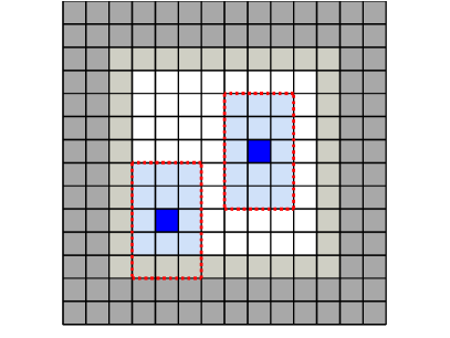
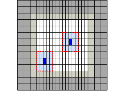
Figure 2.4. An initial T-mesh $\widehat{\mathcal{T}}_{0}^{\rm ext}$ in 2D (left) with $(p_{1},p_{2})=(3,3)$ and its first uniform refinement (right) are depicted. The sets $\widehat{\Omega}$, $\widehat{\Omega}^{\rm act}$, and $\widehat{\Omega}^{\rm ext}$ are highlighted in white, light gray, and dark gray, respectively. For each of the four blue elements, the corresponding neighbors are shown in light blue. According to definition (2.18), the neighbors are all elements in $\overline{\widehat{\Omega}}$ with non-empty intersection with the rectangles indicated in red.

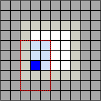
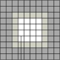
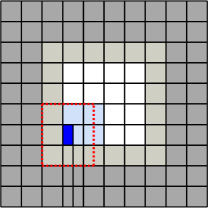
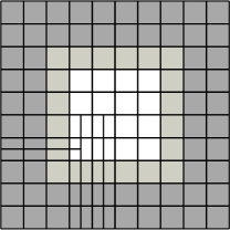
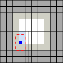
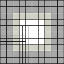
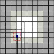
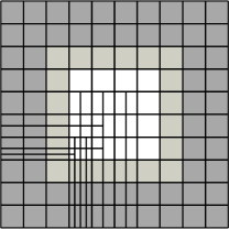
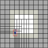
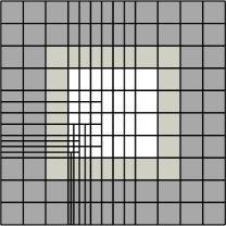
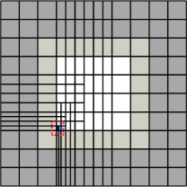
Figure 2.5. An initial T-mesh $\widehat{\mathcal{T}}_{0}^{\rm ext}$ in 2D (top left) with $(p_{1},p_{2})=(3,3)$ and its first five refinements towards the lower left corner of $\widehat{\Omega}$ are depicted. The sets $\widehat{\Omega}$, $\widehat{\Omega}^{\rm act}$, and $\widehat{\Omega}^{\rm ext}$ are highlighted in white, light gray, and dark gray, respectively. Every second picture shows the element (in blue) that is marked to obtain the next mesh. Its neighbors are shown in light blue. According to definition (2.18), the neighbors are all elements in $\overline{\widehat{\Omega}}$ with non-empty intersection with the rectangles indicated in red.

Algorithm 2.1.

Input: T-mesh $\widehat{\mathcal{T}}_{\bullet}$, marked elements $\widehat{\mathcal{M}}_{\bullet}=:\widehat{\mathcal{M}}_{\bullet}^{(0)}\subseteq\widehat{\mathcal{T}}_{\bullet}$.

• Iterate the following steps (a)–(b) for $j=0,1,2,\dots$ until $\widehat{\mathcal{U}}_{\bullet}^{(j)}=\emptyset$:

  • Define $\widehat{\mathcal{U}}_{\bullet}^{(j)}:=\bigcup_{\widehat{T}\in\widehat{\mathcal{M}}_{\bullet}^{(j)}}\boldsymbol{\rm N}^{\rm bad}(\widehat{T})\setminus\widehat{\mathcal{M}}_{\bullet}^{(j)}$.

  • Define $\widehat{\mathcal{M}}_{\bullet}^{(j+1)}:=\widehat{\mathcal{M}}_{\bullet}^{(j)}\cup\widehat{\mathcal{U}}_{\bullet}^{(j)}$.

• Bisect all $\widehat{T}\in\widehat{\mathcal{M}}_{\bullet}^{(j)}$ via ${\tt bisect}_{{\rm level}(\widehat{T})+1-\underline{{\rm level}(\widehat{T})}}$ and obtain a finer T-mesh

  $${\tt refine}(\widehat{\mathcal{T}}_{\bullet},\widehat{\mathcal{M}}_{\bullet}):=\widehat{\mathcal{T}}_{\bullet}\setminus\widehat{\mathcal{M}}_{\bullet}^{(j)}\cup\bigcup\big{\{}{\tt bisect}_{{\rm level}(\widehat{T})+1-\underline{{\rm level}(\widehat{T})}}(\widehat{T})\,:\,\widehat{T}\in\widehat{\mathcal{M}}_{\bullet}^{(j)}\big{\}},$$ (2.22)

  where we recall from (2.4) that $\underline{{\rm level}(\widehat{T})}=\lfloor{\rm level}(\widehat{T})/d\rfloor d$.

Output: Refined mesh ${\tt refine}(\widehat{\mathcal{T}}_{\bullet},\widehat{\mathcal{M}}_{\bullet})$.

Remark 2.2.

The additional bisection of neighbors (and their neighbors, etc.) of marked elements is required to ensure local quasi-uniformity (see (2.24)–(2.25) below) and analysis-suitability in the sense of [BdVBSV13, Mor16] for $d=2,3$, respectively. For $d=2$, the latter is characterized by the assumption that horizontal T-junction extensions do not intersect vertical ones. In particular, this yields linear independence of the set of B-splines $\big{\{}\widehat{B}_{\bullet,z}\,:\,z\in\widehat{\mathcal{N}}^{\rm act}_{\bullet}\big{\}}$; see Section 2.3.

For any T-mesh $\widehat{\mathcal{T}}_{\bullet}$, we define ${\tt refine}(\widehat{\mathcal{T}}_{\bullet})$ as the set of all T-meshes $\widehat{\mathcal{T}}_{\circ}$ such that there exist T-meshes $\widehat{\mathcal{T}}_{(0)},\dots,\widehat{\mathcal{T}}_{(J)}$ and marked elements $\widehat{\mathcal{M}}_{(0)},\dots,\widehat{\mathcal{M}}_{(J-1)}$ with $\widehat{\mathcal{T}}_{\circ}=\widehat{\mathcal{T}}_{(J)}={\tt refine}(\widehat{\mathcal{T}}_{(J-1)},\widehat{\mathcal{M}}_{(J-1)}),\dots,\widehat{\mathcal{T}}_{(1)}={\tt refine}(\widehat{\mathcal{T}}_{(0)},\widehat{\mathcal{M}}_{(0)})$, and $\widehat{\mathcal{T}}_{(0)}=\widehat{\mathcal{T}}_{\bullet}$; see Figure 2.5 for some refined meshes. Here, we formally allow $J=0$, i.e., $\widehat{\mathcal{T}}_{\bullet}\in{\tt refine}(\widehat{\mathcal{T}}_{\bullet})$. Finally, we define the set of all admissible T-meshes as

$$\widehat{\mathbb{T}}:={\tt refine}(\widehat{\mathcal{T}}_{0}).$$ (2.23)

For any admissible $\widehat{\mathcal{T}}_{\bullet}\in\widehat{\mathbb{T}}$, [MP15, remark after Definition 2.4 and Lemma 2.14] proves for $d=2$ that

$$|{\rm level}(\widehat{T})-{\rm level}(\widehat{T}^{\prime})|\leq 1\quad\text{for all }\widehat{T},\widehat{T}^{\prime}\in\widehat{\mathcal{T}}_{\bullet}\text{ with }\widehat{T}^{\prime}\in\boldsymbol{\rm N}_{\bullet}(\widehat{T}),$$ (2.24)

as well as

$$\big{\{}\widehat{T}^{\prime}\in\widehat{\mathcal{T}}_{\bullet}\,:\,\widehat{T}\cap\widehat{T}^{\prime}\neq\emptyset\big{\}}\subseteq\boldsymbol{\rm N}_{\bullet}(\widehat{T})\quad\text{for all }\widehat{T}\in\widehat{\mathcal{T}}_{\bullet}.$$ (2.25)

Similarly, [Mor16, Lemma 3.5] proves (2.24)–(2.25) for $d=3$.

Remark 2.3.

As any element $\widehat{T}\in\widehat{\mathcal{T}}_{\bullet}\in\mathbb{T}$ of level $k$ is essentially of size $2^{-k/2}$ if $d=2$ and $2^{-k/3}$ if $d=3$, the definition of $\boldsymbol{\rm N}_{\bullet}(\widehat{T})$ and (2.24)–(2.25) yield that the number $\#\boldsymbol{\rm N}_{\bullet}(\widehat{T})$ is uniformly bounded independently of the level. Moreover, for $d=2$, [MP15, remark after Definition 2.4] states that whenever $\widehat{T}$ is bisected (in direction $k+1-\underline{k}$), the resulting sons $\widehat{T}_{1},\widehat{T}_{2}$ in the refined mesh $\widehat{\mathcal{T}}_{\circ}$ satisfy that $\boldsymbol{\rm N}_{\circ}(\widehat{T}_{i})\setminus\{\widehat{T}_{1},\widehat{T}_{2}\}\subseteq\boldsymbol{\rm N}_{\bullet}(\widehat{T})\setminus\{\widehat{T}\}$. One elementarily sees that this inclusion also holds for $d=3$. The latter two properties allow for an efficient implementation of Algorithm 2.1, where the neighbors of all elements in the current mesh are stored in a suitable data structure and updated after each bisection.

2.3. Basis of $\widehat{\mathcal{X}}_{\bullet}$

First, we emphasize that for general T-meshes $\widehat{\mathcal{T}}_{\bullet}$ as in Section 2.1, the set $\big{\{}\widehat{B}_{\bullet,z}\,:\,z\in\widehat{\mathcal{N}}^{\rm act}_{\bullet}\big{\}}$ is not necessarily a basis of the corresponding T-spline space $\widehat{\mathcal{Y}}_{\bullet}$ since it is not necessarily linearly independent; see [BCS10] for a counter example. According to [BdVBSV14, Proposition 7.4], a sufficient criterion for linear independence of a set of B-splines is dual-compatibility: We say that $\big{\{}\widehat{B}_{\bullet,z}\,:\,z\in\widehat{\mathcal{N}}_{\bullet}\big{\}}$ is dual-compatible if for all $z,z^{\prime}\in\widehat{\mathcal{N}}_{\bullet}$ with $|\widehat{B}_{\bullet,z}\cap\widehat{B}_{\bullet,z^{\prime}}|>0$, the corresponding local knot vectors are at least in one direction aligned, i.e., there exists $i\in\{1,\dots,d\}$ such that $\widehat{\mathcal{K}}^{\rm loc}_{\bullet,i}(z)$ and $\widehat{\mathcal{K}}^{\rm loc}_{\bullet,i}(z^{\prime})$ are both sub-vectors of one common sorted vector $\widehat{\mathcal{K}}$.

We stress that admissible meshes yield dual-compatible B-splines, where the local knot vectors are even aligned in at least two directions for $d=3$, and thus linearly independent B-splines. Indeed, [MP15, Theorem 3.6] and [Mor16, Theorem 5.3] prove analysis-suitability (see Remark 2.2) for $d=2$ and $d=3$, respectively. According to [BdVBSV14, Theorem 7.16] for $d=2$ and [Mor16, Theorem 6.6] for $d=3$, this implies the stated dual-compatibility. To be precise, [Mor16] defines the space of T-splines differently as the span of $\big{\{}\widehat{B}_{\bullet,z}\,:\,z\in\widehat{\mathcal{N}}_{\bullet}^{\rm act}\cap\overline{\widehat{\Omega}}\big{\}}$ and shows that this set is dual-compatible. The functions in this set are not only zero on the boundary $\partial\widehat{\Omega}$, but also some of their derivatives vanish there since the maximal multiplicity in the used local knot vectors is at most $p_{i}$ in each direction; see, e.g., [dB01, Section 6]. Nevertheless, the proofs immediately generalize to our standard definition of T-splines. The following lemma provides a basis of $\widehat{\mathcal{X}}_{\bullet}$.

Lemma 2.4.

Let $\widehat{\mathcal{T}}_{\bullet}\in\widehat{\mathbb{T}}$ be an arbitrary admissible T-mesh in the parameter domain $\widehat{\Omega}$. Then, $\big{\{}\widehat{B}_{\bullet,z}\,:\,z\in\widehat{\mathcal{N}}^{\rm act}_{\bullet}\setminus\partial\widehat{\Omega}^{\rm act}\big{\}}$ is a basis of $\widehat{\mathcal{X}}_{\bullet}$.

Proof.

Since we already know that the set $\big{\{}\widehat{B}_{\bullet,z}\,:\,z\in\widehat{\mathcal{N}}^{\rm act}_{\bullet}\setminus\partial\widehat{\Omega}^{\rm act}\big{\}}$ is linearly independent, we only have to show that it generates $\widehat{\mathcal{X}}_{\bullet}$.

Step 1: We recall that the one-dimensional B-spline $\widehat{B}(\cdot|{\color[rgb]{0,0,0}}_{0},\dots,{\color[rgb]{0,0,0}}_{p+1})$ induced by a sorted knot vector $({\color[rgb]{0,0,0}}_{0},\dots,{\color[rgb]{0,0,0}}_{p+1})\in{\mathbb{R}}^{p+2}$ is positive on the interval $({\color[rgb]{0,0,0}}_{0},{\color[rgb]{0,0,0}}_{p+1})$. It does not vanish at ${\color[rgb]{0,0,0}}_{0}$ if and only if ${\color[rgb]{0,0,0}}_{0}=\dots={\color[rgb]{0,0,0}}_{p}$, and it does not vanish at ${\color[rgb]{0,0,0}}_{p+1}$ if and only if ${\color[rgb]{0,0,0}}_{1}=\dots={\color[rgb]{0,0,0}}_{p+1}$. In particular, for all $z\in\widehat{\mathcal{N}}_{\bullet}^{\rm act}$, this and the tensor-product structure of $\widehat{B}_{\bullet,z}$ yield that $\widehat{B}_{\bullet,z}|_{\partial\widehat{\Omega}}\neq 0$ if and only if $z{\color[rgb]{0,0,0}}\partial\widehat{\Omega}^{\rm act}$; see also Figure (2.3). This shows that

$${\rm span}\big{\{}\widehat{B}_{\bullet,z}\,:\,z\in\widehat{\mathcal{N}}^{\rm act}_{\bullet}\setminus\partial\widehat{\Omega}^{\rm act}\big{\}}\subseteq\widehat{\mathcal{X}}_{\bullet}.$$ (2.26)

Step 2: To see the other inclusion, let $\widehat{V}_{\bullet}\in\widehat{\mathcal{X}}_{\bullet}$. Then, there exists a representation of the form $\widehat{V}_{\bullet}=\sum_{z\in\widehat{\mathcal{N}}_{\bullet}^{\rm act}}c_{z}\widehat{B}_{\bullet,z}$. Let $\widehat{E}$ be an arbitrary facet of the boundary $\partial\widehat{\Omega}$ and $\widehat{E}^{\rm act}$ its extension onto $\partial\widehat{\Omega}^{\rm act}$, i.e.,

$$\widehat{E} :=\prod_{j=1}^{i-1}[0,N_{j}]\times\{\widehat{e}\}\times\prod_{j=i+1}^{d}[0,N_{j}],$$

$$\widehat{E}^{\rm act} :=\prod_{j=1}^{i-1}[-(p_{j}-1)/2,N_{j}+(p_{j}-1)/2]\times\{\widehat{e}^{\,{\rm act}}\}\times\prod_{j=i+1}^{d}[-(p_{j}-1)/2,N_{j}+(p_{j}-1)/2],$$

with $i\in\{1,\dots,d\}$, $\widehat{e}:=0$ and $\widehat{e}^{\,{\rm act}}:=-(p_{i}-1)/2$, or $\widehat{e}:=N_{i}$ and $\widehat{e}^{\,{\rm act}}:=N_{i}+(p_{i}-1)/2$. Restricting onto $\widehat{E}$ and using the argument from Step 1, we derive that

$$0=\widehat{V}_{\bullet}|_{\widehat{E}}=\sum_{z\in\widehat{\mathcal{N}}_{\bullet}^{\rm act}}c_{z}\widehat{B}_{\bullet,z}|_{\widehat{E}}=\sum_{z\in\widehat{\mathcal{N}}_{\bullet}^{\rm act}\cap\widehat{E}^{\rm act}}c_{z}\widehat{B}_{\bullet,z}|_{\widehat{E}}.$$

For $d=2$, the set $\big{\{}\widehat{B}_{\bullet,z}|_{\widehat{E}}\,:\,z\in\widehat{\mathcal{N}}_{\bullet}^{\rm act}\cap\widehat{E}^{\rm act}\big{\}}$ coincides (up to the domain of definition) with the set of $(d-1)$-dimensional B-splines corresponding to the global knot vector $\widehat{\mathcal{K}}_{\bullet,i}^{\rm gl}((0,0))$ if $\widehat{e}=0$ and $\widehat{\mathcal{K}}_{\bullet,i}^{\rm gl}((N_{1},N_{2}))$ if $\widehat{e}=N_{i}$; see, e.g., [dB01, Section 2] for a precise definition of the set of B-splines associated to some global knot vector. It is well-known that these functions are linearly independent, wherefore we derive that $c_{z}=0$ for the corresponding coefficients.

For $d=3$, the set $\big{\{}\widehat{B}_{\bullet,z}|_{\widehat{E}}\,:\,z\in\widehat{\mathcal{N}}_{\bullet}^{\rm act}\cap\widehat{E}^{\rm act}\big{\}}$ coincides (up to the domain of definition) with the set of $(d-1)$-dimensional B-splines corresponding to the $(d-1)$-dimensional T-mesh

$$\widehat{\mathcal{T}}_{\bullet}^{\rm ext}|_{\widehat{E}^{\rm ext}}:=\Big{\{}\prod_{\begin{subarray}{c}j=1\\ j\neq i\end{subarray}}^{i-1}[a_{j},b_{j}]:\prod_{j=1}^{d}[a_{j},b_{j}]\in\widehat{\mathcal{T}}^{\rm ext}_{\bullet}\wedge a_{i}=\widehat{e}\Big{\}}.$$ (2.27)

We have already mentioned that [Mor16, Theorem 5.3 and Theorem 6.6] shows that the local knot vectors of the B-spline basis of $\widehat{\mathcal{Y}}_{\bullet}$ are even aligned in at least two directions. In particular, the knot vectors of the B-splines corresponding to the mesh $\widehat{\mathcal{T}}_{\bullet}^{\rm ext}|_{\widehat{E}^{\rm ext}}$ are aligned in at least one direction. This yields dual-compatibility and thus linear independence of these B-splines, which concludes that $c_{z}=0$ for the corresponding coefficients. Since $\partial\widehat{\Omega}^{\rm act}$ is the union of all its facets and $\widehat{E}$ was arbitrary, this concludes that $c_{z}=0$ for all $z\in\widehat{\mathcal{N}}_{\bullet}^{\rm act}\cap\partial\widehat{\Omega}^{\rm act}$ and thus the other inclusion in (2.26). ∎

Finally, we study the support of the basis functions of $\widehat{\mathcal{Y}}_{\bullet}$ (and thus of $\widehat{\mathcal{X}}_{\bullet}$). To this end, we define for $\widehat{\mathcal{T}}_{\bullet}\in\widehat{\mathbb{T}}$ and $\widehat{\omega}\subseteq\overline{\widehat{\Omega}}$, the patches of order $k\in{\mathbb{N}}$ inductively by

$$\pi_{\bullet}^{0}(\widehat{\omega}):=\widehat{\omega},\quad\pi_{\bullet}^{k}(\widehat{\omega}):=\bigcup\big{\{}\widehat{T}\in\widehat{\mathcal{T}}_{\bullet}\,:\,{\widehat{T}}\cap\pi_{\bullet}^{k-1}(\widehat{\omega})\neq\emptyset\big{\}}.$$ (2.28)

Lemma 2.5.

Let $\widehat{\mathcal{T}}_{\bullet}\in\widehat{\mathbb{T}}$, $\widehat{T}\in\widehat{\mathcal{T}}_{\bullet}$, and $z\in\widehat{\mathcal{N}}_{\bullet}^{\rm act}$ with $|\widehat{T}\cap{\rm supp}(\widehat{B}_{\bullet,z})|>0$. Then, there exists a uniform $k_{\rm supp}\in{\mathbb{N}}_{0}$ such that ${\rm supp}(\widehat{B}_{\bullet,z})\subseteq\pi_{\bullet}^{k_{\rm supp}}(\widehat{T})$. Moreover, there exist only $k_{\rm supp}$ nodes $z^{\prime}\in\widehat{\mathcal{N}}_{\bullet}^{\rm act}$ such that $|\widehat{T}\cap{\rm supp}(\widehat{B}_{\bullet,z^{\prime}})|>0$. The constant $k_{\rm supp}$ depends only on $d$ and $(p_{1},\dots,p_{d})$.

Proof.

We prove the assertion in two steps.

Step 1: We prove the first assertion. Without loss of generality, we can assume that $z\in\overline{\widehat{\Omega}}$, since otherwise there exists $z^{\prime\prime}\in\widehat{\mathcal{N}}_{\bullet}^{\rm act}\cap\overline{\widehat{\Omega}}$ (namely the projection of $z$ into $\overline{\widehat{\Omega}}$) such that ${\rm supp}(\widehat{B}_{\bullet,z})\subseteq{\rm supp}(\widehat{B}_{\bullet,z^{\prime\prime}})$ (see (2.14)) and the assertion for $z^{\prime\prime}$ yields that ${\rm supp}(\widehat{B}_{\bullet,z})\subseteq\pi_{\bullet}^{k_{\rm supp}}(\widehat{T})$. Obviously, the support of $\widehat{B}_{\bullet,z}$ can be covered by elements in $\widehat{\mathcal{T}}_{\bullet}$, i.e., ${\rm supp}(\widehat{B}_{\bullet,z})\subseteq\bigcup\widehat{\mathcal{T}}_{\bullet}=\overline{\widehat{\Omega}}$. We show that $|\widehat{T}|\simeq|{\rm supp}(\widehat{B}_{\bullet,z})|$. Let $\widehat{T}_{z}\in\widehat{\mathcal{T}}_{\bullet}$ with $z\in\widehat{T}_{z}$ and thus $\widehat{T}_{z}\subseteq{\rm supp}(\widehat{B}_{\bullet,z})$. Then, (2.24)–(2.25) and the definition of $\widehat{B}_{\bullet,z}$ show that

$$|\widehat{T}_{z}|\simeq|{\rm supp}(\widehat{B}_{\bullet,z})|.$$ (2.29)

Now, let $z_{\widehat{T}}\in\widehat{\mathcal{N}}_{\bullet}^{\rm act}$ with $z_{\widehat{T}}\in\widehat{T}$ and thus $\widehat{T}\subseteq{\rm supp}(\widehat{B}_{\bullet,z_{\widehat{T}}})$. Then, we have that $|{\rm supp}(\widehat{B}_{\bullet,z})\cap{\rm supp}(\widehat{B}_{\bullet,z_{\widehat{T}}})|>0$. Since $\widehat{\mathcal{T}}_{\bullet}$ yields dual-compatible B-splines, the knot lines of $\widehat{B}_{\bullet,z}$ and $\widehat{B}_{\bullet,z_{\widehat{T}}}$ are aligned in one direction. Moreover, due to (2.24)–(2.25), the difference between consecutive knot lines is equivalent to $2^{-{\rm level}(\widehat{T}_{z})/2}$ and $2^{-{\rm level}(\widehat{T})/2}$, respectively. Thus, we obtain that ${\rm level}(\widehat{T}_{z})\simeq{\rm level}(\widehat{T})$ and $|\widehat{T}_{z}|\simeq|\widehat{T}|$. In combination with (2.29), we derive that $|\widehat{T}|\simeq|{\rm supp}(\widehat{B}_{\bullet,z})|$. Since $\widehat{T}$ is arbitrary and ${\rm supp}(\widehat{B}_{\bullet,z})$ is connected, this yields the existence of $k_{\rm supp}^{\prime}\in{\mathbb{N}}_{0}$ with ${\rm supp}(\widehat{B}_{\bullet,z})\subseteq\pi_{\bullet}^{k_{\rm supp}^{\prime}}(\widehat{T})$.

Step 2: We prove the second assertion. First, let $z^{\prime}\in\widehat{\mathcal{N}}_{\bullet}^{\rm act}\cap\overline{\widehat{\Omega}}$. Then, Step 1 gives that $z^{\prime}\in{\rm supp}(\widehat{B}_{\bullet,z^{\prime}})\subseteq\pi_{\bullet}^{k_{\rm supp}}(\widehat{T})$. Therefore, we see that the number of such $z^{\prime}$ is bounded by $\#(\widehat{\mathcal{N}}_{\bullet}^{\rm act}\cap\overline{\widehat{\Omega}}\cap\pi_{\bullet}^{k_{\rm supp}}(\widehat{T}))$. If $z^{\prime}\in\widehat{\mathcal{N}}_{\bullet}^{\rm act}\setminus\overline{\widehat{\Omega}}$, there exists $z^{\prime\prime}\in\widehat{\mathcal{N}}_{\bullet}^{\rm act}\cap\overline{\widehat{\Omega}}$ (namely the projection of $z^{\prime}$ into $\overline{\widehat{\Omega}}$) such that ${\rm supp}(\widehat{B}_{\bullet,{\color[rgb]{0,0,0}{z^{\prime}}}})\subseteq{\rm supp}(\widehat{B}_{\bullet,z^{\prime\prime}})$ and thus $|{\rm supp}(\widehat{T}\cap\widehat{B}_{\bullet,z^{\prime\prime}})|>0$. On the other hand, for given $z^{\prime\prime}\in\widehat{\mathcal{N}}_{\bullet}^{\rm act}\cap\overline{\widehat{\Omega}}$, the number of $z^{\prime}\in\widehat{\mathcal{N}}_{\bullet}^{\rm act}\setminus\overline{\widehat{\Omega}}$ with ${\rm supp}(\widehat{B}_{\bullet,{\color[rgb]{0,0,0}{z^{\prime}}}})\subseteq{\rm supp}(\widehat{B}_{\bullet,z^{\prime\prime}})$ is uniformly bounded by some constant $C>0$ depending only on $d$ and $(p_{1},\dots,p_{d})$; see also Figure 2.3. Altogether, we see that the number of $z^{\prime}\in\widehat{\mathcal{N}}_{\bullet}^{\rm act}$ with $|{\rm supp}(\widehat{B}_{\bullet,z^{\prime}})\cap\widehat{T}|>0$ is bounded by $(1+C)\#(\widehat{\mathcal{N}}_{\bullet}^{\rm act}\cap\overline{\widehat{\Omega}}\cap\pi_{\bullet}^{k_{\rm supp}}(\widehat{T}))$. Due to (2.24)–(2.25), this term is bounded by some uniform constant $k_{\rm supp}^{\prime\prime}\in{\mathbb{N}}_{0}$. Finally, we set $k_{\rm supp}:=\max(k_{\rm supp}^{\prime},k_{\rm supp}^{\prime\prime})$. ∎

2.4. T-meshes and splines in the physical domain $\mathbb{\Omega}$

To transform the definitions in the parameter domain $\widehat{\Omega}$ to the physical domain $\Omega$, we assume as in [GHP17, Section 3.6] that we are given a bi-Lipschitz continuous piecewise $C^{2}$ parametrization

$$\gamma:\overline{\widehat{\Omega}}\to\overline{\Omega}\quad\text{with}\quad\gamma\in W^{1,\infty}({\widehat{\Omega}})\cap C^{2}(\widehat{\mathcal{T}}_{0})\quad\text{and}\quad\gamma^{-1}\in W^{1,\infty}(\Omega)\cap C^{2}({\mathcal{T}}_{0}),$$ (2.30)

where $C^{2}(\widehat{\mathcal{T}}_{0}):=\big{\{}v:\overline{\Omega}\to{\mathbb{R}}\,:\,v|_{\widehat{T}}\in C^{2}(\widehat{T})\text{ for all }\widehat{T}\in\widehat{\mathcal{T}}_{0}\big{\}}$ and $C^{2}({\mathcal{T}}_{0}):=\big{\{}v:\overline{\Omega}\to{\mathbb{R}}\,:\,v|_{T}\in C^{2}(T)\text{ for all }T\in{\mathcal{T}}_{0}\big{\}}$. Consequently, there exists $C_{\gamma}>0$ such that for all $i,j,k\in\{1,\dots,d\}$

$$\begin{split}\Big{\|}\frac{\partial}{\partial t_{j}}\gamma_{i}\Big{\|}_{L^{\infty}(\widehat{\Omega})}\leq C_{\gamma},\quad\Big{\|}\frac{\partial}{\partial x_{j}}(\gamma^{-1})_{i}\Big{\|}_{L^{\infty}(\Omega)}\leq C_{\gamma},\\ \Big{\|}\frac{\partial^{2}}{\partial t_{j}\partial t_{k}}\gamma_{i}\Big{\|}_{L^{\infty}(\widehat{\Omega})}\leq C_{\gamma},\quad\Big{\|}\frac{\partial^{2}}{\partial x_{j}\partial x_{k}}(\gamma^{-1})_{i}\Big{\|}_{L^{\infty}(\Omega)}\leq C_{\gamma},\end{split}$$ (2.31)

where $\gamma_{i}$ resp.  $(\gamma^{-1})_{i}$ denotes the $i$-th component of $\gamma$ resp.  $\gamma^{-1}$ and any second derivative is meant ${\mathcal{T}}_{0}$-elementwise. All previous definitions can now also be made in the physical domain, just by pulling them from the parameter domain via the diffeomorphism $\gamma$. For these definitions, we drop the symbol $\widehat{\cdot}$. Given $\widehat{\mathcal{T}}_{\bullet}\in\widehat{\mathbb{T}}$, the corresponding mesh in the physical domain reads ${\mathcal{T}}_{\bullet}:=\big{\{}\gamma(\widehat{T})\,:\,\widehat{T}\in\widehat{\mathcal{T}}_{\bullet}\big{\}}$. In particular, we have that ${\mathcal{T}}_{0}=\big{\{}\gamma(\widehat{T})\,:\,\widehat{T}\in\widehat{\mathcal{T}}_{0}\big{\}}$. Moreover, let $\mathbb{T}:=\big{\{}{\mathcal{T}}_{\bullet}\,:\,\widehat{\mathcal{T}}_{\bullet}\in\widehat{\mathbb{T}}\big{\}}$ be the set of admissible meshes in the physical domain. If now $\mathcal{M}_{\bullet}\subseteq{\mathcal{T}}_{\bullet}$ with ${\mathcal{T}}_{\bullet}\in\mathbb{T}$, we abbreviate $\widehat{\mathcal{M}}_{\bullet}:=\big{\{}\gamma^{-1}(T)\,:\,T\in\mathcal{M}_{\bullet}\big{\}}$ and define ${\tt refine}({\mathcal{T}}_{\bullet},\mathcal{M}_{\bullet}):=\big{\{}\gamma(\widehat{T})\,:\,\widehat{T}\in{\tt refine}(\widehat{\mathcal{T}}_{\bullet},\widehat{\mathcal{M}}_{\bullet})\big{\}}$. For ${\mathcal{T}}_{\bullet}\in\mathbb{T}$, let ${\mathcal{Y}}_{\bullet}:=\big{\{}\widehat{V}_{\bullet}\circ\gamma^{-1}\,:\,\widehat{V}_{\bullet}\in\widehat{\mathcal{Y}}_{\bullet}\big{\}}$ be the corresponding space of T-splines, and ${\mathcal{X}}_{\bullet}:=\big{\{}\widehat{V}_{\bullet}\circ\gamma^{-1}\,:\,\widehat{V}_{\bullet}\in\widehat{\mathcal{X}}_{\bullet}\big{\}}$ the corresponding space of T-splines which vanish on the boundary. By regularity of $\gamma$, we especially obtain that

$${\mathcal{X}}_{\bullet}\subset\big{\{}v\in H_{0}^{1}(\Omega)\,:\,v|_{T}\in H^{2}(T)\text{ for all }T\in{\mathcal{T}}_{\bullet}\big{\}}.$$ (2.32)

Let $U_{\bullet}\in{\mathcal{X}}_{\bullet}$ be the corresponding Galerkin approximation to the solution $u\in H^{1}_{0}(\Omega)$, i.e.,

$$\langle U_{\bullet}\,,\,V_{\bullet}\rangle_{\mathcal{L}}=\int_{\Omega}fV_{\bullet}-\boldsymbol{f}\cdot\nabla V_{\bullet}\,dx\quad\text{for all }V_{\bullet}\in{\mathcal{X}}_{\bullet}.$$ (2.33)

We note the Galerkin orthogonality

$$\langle u-U_{\bullet}\,,\,V_{\bullet}\rangle_{\mathcal{L}}=0\quad\text{for all }V_{\bullet}\in{\mathcal{X}}_{\bullet}$$ (2.34)

as well as the resulting Céa-type quasi-optimality

$$\|u-U_{\bullet}\|_{H^{1}(\Omega)}\leq C_{\text{C\'{e}a}}\min_{V_{\bullet}\in{\mathcal{X}}_{\bullet}}\|u-V_{\bullet}\|_{H^{1}(\Omega)}\text{ with }C_{\text{C\'{e}a}}:=\textstyle\frac{\|\textit{{A}}\|_{L^{\infty}(\Omega)}\!+\!\|\textit{{b}}\|_{L^{\infty}(\Omega)}\!+\!\|c\|_{L^{\infty}(\Omega)}}{C_{\rm ell}}.$$ (2.35)

2.5. Error estimator

Let ${\mathcal{T}}_{\bullet}\in\mathbb{T}$ and $T_{1}\in{\mathcal{T}}_{\bullet}$. For almost every $x\in\partial T_{1}\cap\Omega$, there exists a unique element $T_{2}\in{\mathcal{T}}_{\bullet}$ with $x\in T_{1}\cap T_{2}$. We denote the corresponding outer normal vectors by $\nu_{1}$ resp. $\nu_{2}$ and define the normal jump as

$$[(\textit{{A}}\nabla U_{\bullet}+\boldsymbol{f})\cdot\nu](x)=(\textit{{A}}\nabla U_{\bullet}+\boldsymbol{f})|_{T_{1}}(x)\cdot\nu_{1}(x)+(\textit{{A}}\nabla U_{\bullet}+\boldsymbol{f})|_{T^{\prime}}(x)\cdot\nu_{2}(x).$$ (2.36)

With this definition, we employ the residual a posteriori error estimator

$$\eta_{\bullet}:=\eta_{\bullet}({\mathcal{T}}_{\bullet})\quad\text{with}\quad\eta_{\bullet}({\mathcal{S}}_{\bullet})^{2}:=\sum_{T\in{\mathcal{S}}_{\bullet}}\eta_{\bullet}(T)^{2}\text{ for all }{\mathcal{S}}_{\bullet}\subseteq{\mathcal{T}}_{\bullet},$$ (2.37a)

where, for all $$T\in{\mathcal{T}}_{\bullet}$$, the local refinement indicators read

$$\begin{split}\eta_{\bullet}(T)^{2}&:=|T|^{2/d}\|f+{\rm div}(\textit{{A}}\nabla U_{\bullet}+\boldsymbol{f})-\textit{{b}}\cdot\nabla U_{\bullet}-cU_{\bullet}\|_{L^{2}(T)}^{2}\\ &\quad+|T|^{1/d}\|[(\textit{{A}}\nabla U_{\bullet}+\boldsymbol{f})\cdot\nu]\|_{L^{2}(\partial T\cap\Omega)}^{2}.\end{split}$$ (2.37b)

We refer, e.g., to the monographs [AO00, Ver13] for the analysis of the residual a posteriori error estimator (2.37) in the frame of standard FEM with piecewise polynomials of fixed order.

Remark 2.6.

If ${\mathcal{X}}_{\bullet}\subset C^{1}(\Omega)$, then the jump contributions in (2.37) vanish and $\eta_{\bullet}(T)$ consists only of the volume residual.

2.6. Adaptive algorithm

We consider the common formulation of an adaptive mesh-refining algorithm; see, e.g., Algorithm 2.2 of [CFPP14].

Algorithm 2.7.

Input: Adaptivity parameter $0<\theta\leq 1$ and marking constant $C_{\rm min}\geq 1$.
Loop: For each $\ell=0,1,2,\dots$, iterate the following steps (i)–(iv):

• Compute Galerkin approximation $U_{\ell}\in{\mathcal{X}}_{\ell}$.

• Compute refinement indicators $\eta_{\ell}({T})$ for all elements ${T}\in{\mathcal{T}}_{\ell}$.

• Determine a set of marked elements $\mathcal{M}_{\ell}\subseteq{\mathcal{T}}_{\ell}$ with $\theta\,\eta_{\ell}^{2}\leq\eta_{\ell}(\mathcal{M}_{\ell})^{2}$ which has up to the multiplicative constant $C_{\rm min}$ minimal cardinality.

• Generate refined mesh ${\mathcal{T}}_{\ell+1}:={\tt refine}({\mathcal{T}}_{\ell},\mathcal{M}_{\ell})$.

Output: Sequence of successively refined meshes ${\mathcal{T}}_{\ell}$ and corresponding Galerkin approximations $U_{\ell}$ with error estimators $\eta_{\ell}$ for all $\ell\in{\mathbb{N}}_{0}$.

Remark 2.8.

For the sake of simplicity, we assume that $U_{\ell}$ is computed exactly. However, according to [CFPP14, Section 7], the forthcoming optimality analysis remains valid if $U_{\ell}$ is replaced by an approximation $\widetilde{U}_{\ell}\in{\mathcal{X}}_{\ell}$ such that

$$\|U_{\ell}-\widetilde{U}_{\ell}\|_{\mathcal{L}}\leq\vartheta\eta_{\ell}(\widetilde{U}_{\ell})$$ (2.38)

with the energy norm $\|\cdot\|_{\mathcal{L}}^{2}:=\langle\cdot\,,\,\cdot\rangle_{\mathcal{L}}$, the error estimator $\eta_{\ell}(\widetilde{U}_{\ell})$ defined analogously as in (2.37), and a sufficiently small but fixed adaptivity parameter $0<\vartheta<1$. In practice, (2.38) can be efficiently realized if one preconditions the arising linear system appropriately and then solves it iteratively; see [FHPS19] in case of the boundary element method. Assuming $\mathcal{L}$ to be symmetric, i.e., $\textit{{b}}=0$, one employs PCG-iterations [GvL12] starting from $\widetilde{U}_{\ell}^{0}:=\widetilde{U}_{\ell-1}$ with $\widetilde{U}_{-1}:=0$ until

$$\|\widetilde{U}_{\ell}^{j}-\widetilde{U}_{\ell}^{j-1}\|_{\mathcal{L}}\leq\vartheta^{\prime}\eta_{\ell}(\widetilde{U}_{\ell}^{j}),$$ (2.39)

and $\widetilde{U}_{\ell}$ is defined as the final PCG-iterate $\widetilde{U}_{\ell}^{j}$. For analysis-suitable T-splines and the Poisson model problem, appropriate preconditioners have recently been developed in [CV20]. At least for the Poisson model problem, this gives rise to an extended version of Algorithm 2.7 which does not only converge at optimal rate with respect to the number of mesh elements, but also with respect to the overall computational cost; see [GPS19b] for a recent development.

2.7. Data oscillations

We fix polynomial orders $(q_{1},\dots,q_{d})$ and define for ${\mathcal{T}}_{\bullet}\in\mathbb{T}$ the space of transformed polynomials

$$\mathcal{P}(\Omega):=\big{\{}\widehat{V}\circ\gamma\,:\,\widehat{V}\text{ is a tensor-polynomial of order }(q_{1},\dots,q_{d})\big{\}}.$$ (2.40)

Remark 2.9.

In order to obtain higher-order oscillations, the natural choice of the polynomial orders is $q_{i}\geq 2p_{i}-1$ for $i\in\{1\,\dots,d\}$; see, e.g., [NV12, Section 3.1]. If ${\mathcal{X}}_{\bullet}\subset C^{1}(\Omega)$, it is sufficient to choose $q_{i}\geq 2p_{i}-2$; see Remark 2.10.

Let ${\mathcal{T}}_{\bullet}\in\mathbb{T}$. For $T\in{\mathcal{T}}_{\bullet}$, we define the $L^{2}$-orthogonal projection $P_{\bullet,T}:L^{2}(T)\to\big{\{}{W}|_{T}\,:\,{W}\in\mathcal{P}(\Omega)\big{\}}$. For an interior edge $E\in\mathcal{E}_{\bullet,T}:=\big{\{}T\cap T^{\prime}\,:\,T^{\prime}\in{\mathcal{T}}_{\bullet}\wedge{\rm dim}(T\cap T^{\prime})=d-1\big{\}}$, we define the $L^{2}$-orthogonal projection $P_{\bullet,E}:L^{2}(E)\to\big{\{}{W}|_{E}\,:\,{W}\in\mathcal{P}(\Omega)\big{\}}$. Note that $\bigcup\mathcal{E}_{\bullet,T}=\overline{\partial T\cap\Omega}$. For $V_{\bullet}\in{\mathcal{X}}_{\bullet}$, we define the corresponding oscillations

$${\rm osc}_{\bullet}(V_{\bullet}):={\rm osc}_{\bullet}(V_{\bullet},{\mathcal{T}}_{\bullet})\quad\text{with}\quad{\rm osc}_{\bullet}({{V_{\bullet}}},{\mathcal{S}}_{\bullet})^{2}:=\sum_{T\in{\mathcal{S}}_{\bullet}}{\rm osc}_{\bullet}({{V_{\bullet}}},T)^{2}\text{ for all }{\mathcal{S}}_{\bullet}\subseteq{\mathcal{T}}_{\bullet},$$ (2.41a)

where, for all $$T\in{\mathcal{T}}_{\bullet}$$, the local oscillations read

$$\begin{split}{\rm osc}_{\bullet}({{V_{\bullet}}},T)^{2}&:=|T|^{2/d}\|(1-P_{\bullet,T})(f+{\rm div}(\textit{{A}}\nabla V_{\bullet}+\boldsymbol{f})-\textit{{b}}\cdot\nabla V_{\bullet}-cV_{\bullet})\|_{L^{2}(T)}^{2}\\ &\quad+\sum_{E\in\mathcal{E}_{\bullet,T}}|T|^{1/d}\|(1-P_{\bullet,E})[(\textit{{A}}\nabla V_{\bullet}+\boldsymbol{f})\cdot\nu]\|_{L^{2}(E)}^{2}.\end{split}$$ (2.41b)

We refer, e.g., to [NV12] for the analysis of oscillations in the frame of standard FEM with piecewise polynomials of fixed order.

Remark 2.10.

If ${\mathcal{X}}_{\bullet}\subset C^{1}(\Omega)$, then the jump contributions in (2.41) vanish and ${\rm osc}_{\bullet}(V_{\bullet},T)$ consists only of the volume oscillations.

2.8. Main result

Let

$$\mathbb{T}(N):=\big{\{}{\mathcal{T}}_{\bullet}\in\mathbb{T}\,:\,\#{\mathcal{T}}_{\bullet}-\#{\mathcal{T}}_{0}\leq N\big{\}}\quad\text{for all }N\in{\mathbb{N}}_{0}.$$ (2.42)

For all $s>0$, define

$$\|u\|_{\mathbb{A}_{s}}:=\sup_{N\in{\mathbb{N}}_{0}}\min_{{\mathcal{T}}_{\bullet}\in\mathbb{T}(N)}(N+1)^{s}\,\eta_{\bullet}\in[0,\infty]$$ (2.43)

and

$$\|u\|_{\mathbb{B}_{s}}:=\sup_{N\in{\mathbb{N}}_{0}}\Big{(}\min_{{\mathcal{T}}_{\bullet}\in\mathbb{T}(N)}(N+1)^{s}\,\inf_{V_{\bullet}\in{\mathcal{X}}_{\bullet}}\big{(}\|u-V_{\bullet}\|_{H^{1}(\Omega)}+{\rm osc}_{\bullet}(V_{\bullet})\big{)}\Big{)}\in[0,\infty].$$ (2.44)

By definition, $\|u\|_{\mathbb{A}_{s}}<\infty$ (or $\|u\|_{\mathbb{B}_{s}}<\infty$) implies that the error estimator $\eta_{\bullet}$ (or the total error) on the optimal meshes ${\mathcal{T}}_{\bullet}$ decays at least with rate ${\mathcal{O}}\big{(}(\#{\mathcal{T}}_{\bullet})^{-s}\big{)}$. The following main theorem states that Algorithm 2.7 reaches each possible rate $s>0$. The proof builds upon the analysis of [GHP17] and is given in Section 3. Generalizations are found in Section 4.

Theorem 2.11.

The following four assertions (i)–(iv) hold:

• The residual error estimator (2.37) satisfies reliability, i.e., there exists a constant $C_{\rm rel}>0$ such that

  $$\|u-U_{\bullet}\|_{H^{1}(\Omega)}+{\rm osc}_{\bullet}\leq C_{\rm rel}\eta_{\bullet}\quad\text{for all }{\mathcal{T}}_{\bullet}\in\mathbb{T}.$$ (2.45)

• The residual error estimator satisfies efficiency, i.e., there exists a constant $C_{\rm eff}>0$ such that

  $$C_{\rm eff}^{-1}\eta_{\bullet}\leq\inf_{V_{\bullet}\in{\mathcal{X}}_{\bullet}}\big{(}\|u-V_{\bullet}\|_{H^{1}(\Omega)}+{\rm osc}_{\bullet}(V_{\bullet})\big{)}.$$ (2.46)

• For arbitrary $0<\theta\leq 1$ and $C_{\rm min}\geq 1$, there exist constants $C_{\rm lin}>0$ and $0<q_{\rm lin}<1$ such that the estimator sequence of Algorithm 2.7 guarantees linear convergence in the sense of

  $$\eta_{\ell+j}^{2}\leq C_{\rm lin}q_{\rm lin}^{j}\eta_{\ell}^{2}\quad\text{for all }j,\ell\in{\mathbb{N}}_{0}.$$ (2.47)

• There exists a constant $0<\theta_{\rm opt}\leq 1$ such that for all $0<\theta<\theta_{\rm opt}$, all $C_{\rm min}\geq 1$, and all $s>0$, there exist constants $c_{\rm opt},C_{\rm opt}>0$ such that

  $$c_{\rm opt}\|u\|_{\mathbb{A}_{s}}\leq\sup_{\ell\in{\mathbb{N}}_{0}}{(\#{\mathcal{T}}_{\ell}-\#{\mathcal{T}}_{0}+1)^{s}}\,{\eta_{\ell}}\leq C_{\rm opt}\|u\|_{\mathbb{A}_{s}},$$ (2.48)

  i.e., the estimator sequence will decay with each possible rate $s>0$.

The constants $C_{\rm rel},C_{\rm eff},C_{\rm lin},q_{\rm lin},\theta_{\rm opt},$ and $C_{\rm opt}$ depend only on $d$, the coefficients of the differential operator $\mathcal{L}$, ${\rm diam}(\Omega)$, $C_{\rm\gamma}$, and $(p_{1},\dots,p_{d})$, where $C_{\rm lin},q_{\rm lin}$ depend additionally on $\theta$ and the sequence $(U_{\ell})_{\ell\in{\mathbb{N}}_{0}}$, and $C_{\rm opt}$ depends furthermore on $C_{\rm min}$, and $s>0$. Finally, $c_{\rm opt}$ depends only on $C_{\rm son}$, $\#{\mathcal{T}}_{0}$, and $s$. $\square$

Remark 2.12.

In particular, it holds that

$$C_{\rm eff}^{-1}\|u\|_{\mathbb{A}_{s}}\leq\|u\|_{\mathbb{B}_{s}}\leq C_{\rm rel}\|u\|_{\mathbb{A}_{s}}\quad\text{for all }s>0.$$ (2.49)

If one applies continuous piecewise polynomials of degree $p$ on a triangulation of some polygonal or polyhedral domain $\Omega$ as ansatz space, [GM08] proves that $\|u\|_{\mathbb{B}_{p/d}}<\infty$. The proof requires that $u$ allows for a certain decomposition and that the oscillations are of higher order; see Remark 2.9. In our case, $\|u\|_{\mathbb{A}_{s}}\simeq\|u\|_{\mathbb{B}_{s}}$ depends besides the polynomial degrees $(p_{1},\dots,p_{d})$ also on the (piecewise) smoothness of the parametrization $\gamma$. In practice, $\gamma$ is usually piecewise $C^{\infty}$. Given this additional regularity of $\gamma$, one might expect that the result of [GM08] can be generalized such that $\|u\|_{\mathbb{A}_{s}},\|u\|_{\mathbb{B}_{s}}<\infty$ for $s=\min_{i=1,\dots,d}p_{i}/d$. However, the proof goes beyond the scope of the present work and is left to future research.

Remark 2.13.

Note that almost minimal cardinality of $\mathcal{M}_{\ell}$ in Algorithm 2.7 (iii) is only required to prove optimal convergence behavior (2.48), while linear convergence (2.47) formally allows $C_{\rm min}=\infty$, i.e., it suffices that $\mathcal{M}_{\ell}$ satisfies the Dörfler marking criterion. We refer to [CFPP14, Section 4.3–4.4] for details.

Remark 2.14.

(a) If the bilinear form $\langle\cdot\,,\,\cdot\rangle_{\mathcal{L}}$ is symmetric, $C_{\rm lin}$, $q_{\rm lin}$ as well as $c_{\rm opt}$, $C_{\rm opt}$ are independent of $(U_{\ell})_{\ell\in{\mathbb{N}}_{0}}$; see [GHP17, Remark 4.1].

(b) If the bilinear form $\langle\cdot\,,\,\cdot\rangle_{\mathcal{L}}$ is non-symmetric, there exists an index $\ell_{0}\in{\mathbb{N}}_{0}$ such that the constants $C_{\rm lin}$, $q_{\rm lin}$ as well as $c_{\rm opt}$, $C_{\rm opt}$ are independent of $(U_{\ell})_{\ell\in{\mathbb{N}}_{0}}$ if (2.47)–(2.48) are formulated only for $\ell\geq\ell_{0}$. We refer to the recent work [BHP17, Theorem 19].

Remark 2.15.

Let $h_{\ell}:=\max_{T\in{\mathcal{T}}_{\ell}}|T|^{1/d}$ be the maximal mesh-width. Then, $h_{\ell}\to 0$ as $\ell\to\infty$, ensures that ${\mathcal{X}}_{\infty}:=\overline{\bigcup_{\ell\in{\mathbb{N}}_{0}}{\mathcal{X}}_{\ell}}=H_{0}^{1}(\Omega)$; see [GHP17, Remark 2.7] for the elementary proof. We note that the latter observation allows to follow the ideas of [BHP17] to show that the adaptive algorithm yields optimal convergence even if the bilinear form $\langle\cdot\,,\,\cdot\rangle_{\mathcal{L}}$ is only elliptic up to some compact perturbation provided that the continuous problem is well-posed. This includes, e.g., adaptive FEM for the Helmhotz equation; see [BHP17].

3. Proof of Theorem 2.11

In [GHP17, Section 2], we have identified abstract properties of the underlying meshes, the mesh-refinement, the finite element spaces, and the oscillations which imply Theorem 2.11; see [Gan17, Section 4.2–4.3] for more details. We mention that [GHP17, Gan17] actually only treat the case $\boldsymbol{f}=0$, but the corresponding proofs immediately extend to more general $\boldsymbol{f}$ as in Section 1.2. In the remainder of this section, we recapitulate these properties and verify them for our considered T-spline setting. For their formulation, we define for ${\mathcal{T}}_{\bullet}\in\mathbb{T}$ and $\omega\subseteq\overline{\Omega}$, the patches of order $k\in{\mathbb{N}}$ inductively by

$$\pi_{\bullet}^{0}(\omega):=\omega,\quad\pi_{\bullet}^{k}(\omega):=\bigcup\big{\{}T\in{\mathcal{T}}_{\bullet}\,:\,{T}\cap\pi_{\bullet}^{k-1}(\omega)\neq\emptyset\big{\}}.$$ (3.1)

The corresponding set of elements is

$$\Pi_{\bullet}^{k}(\omega):=\big{\{}T\in{\mathcal{T}}_{\bullet}\,:\,{T}\subseteq\pi_{\bullet}^{k}(\omega)\big{\}},\quad\text{i.e.,}\quad\pi_{\bullet}^{k}(\omega)=\bigcup\Pi_{\bullet}^{k}(\omega){\text{ for }k>0}.$$ (3.2)

To abbreviate notation, we let $\pi_{\bullet}(\omega):=\pi_{\bullet}^{1}(\omega)$ and $\Pi_{\bullet}(\omega):=\Pi_{\bullet}^{1}(\omega)$. For ${\mathcal{S}}_{\bullet}\subseteq{\mathcal{T}}_{\bullet}$, we define $\pi_{\bullet}^{k}({\mathcal{S}}_{\bullet}):=\pi_{\bullet}^{k}(\bigcup{\mathcal{S}}_{\bullet})$ and $\Pi_{\bullet}^{k}({\mathcal{S}}_{\bullet}):=\Pi_{\bullet}^{k}(\bigcup{\mathcal{S}}_{\bullet})$.

3.1. Mesh properties

We show that there exist $C_{\rm locuni},C_{\rm patch},C_{\rm trace},C_{\rm dual}>0$ such that all meshes ${\mathcal{T}}_{\bullet}\in\mathbb{T}$ satisfy the following four properties (M1)–(M4):

1. Local quasi-uniformity. For all $T\in{\mathcal{T}}_{\bullet}$ and all $T^{\prime}\in\Pi_{\bullet}(T)$, it holds that $C_{\rm locuni}^{-1}|T^{\prime}|\leq|T|\leq C_{\rm locuni}\,|T^{\prime}|$, i.e., neighboring elements have comparable size.

2. Bounded element patch. For all $T\in{\mathcal{T}}_{\bullet}$, it holds that $\#\Pi_{\bullet}(T)\leq C_{\rm patch}$, i.e., the number of elements in a patch is uniformly bounded.

3. Trace inequality. For all $T\in{\mathcal{T}}_{\bullet}$ and all $v\in H^{1}(\Omega)$, it holds that $\|v\|_{L^{2}(\partial T)}^{2}\leq C_{\rm trace}\big{(}|T|^{-1/d}\|v\|_{L^{2}(T)}^{2}+|T|^{1/d}\|\nabla v\|_{L^{2}(T)}^{2}\big{)}.$

4. Local estimate in dual norm: For all $T\in{\mathcal{T}}_{\bullet}$ and all $w\in L^{2}(T)$, it holds that $|T|^{-1/d}\|w\|_{H^{-1}(T)}\leq C_{\rm dual}\|w\|_{L^{2}(T)},$ where $\|{w}\|_{H^{-1}(T)}:=\sup\big{\{}\int_{T}{w}v\,dx\,:\,v\in H_{0}^{1}(T)\wedge\|\nabla v\|_{L^{2}(T)}=1\big{\}}$.

Remark 3.1.

In usual applications, where $T\in{\mathcal{T}}_{\bullet}$ have simple shapes, the properties (M3)–(M4) are naturally satisfied; see, e.g., [Gan17, Section 4.2.1].

To see (M1)–(M4), let ${\mathcal{T}}_{\bullet}\in\mathbb{T}$. Then, (2.24)–(2.25) imply local quasi-uniformity (M1) in the parameter domain, which transfers with the help of the regularity (2.31) of $\gamma$ immediately to the physical domain. The constant $C_{\rm locuni}$ depends only on the dimension $d$ and the constant $C_{\rm\gamma}$. Moreover, (2.24)–(2.25) yield uniform boundedness of the number of elements in a patch, i.e., (M2), where $C_{\rm patch}$ depends only on $d$.

Regularity (2.31) of $\gamma$ shows that it is sufficient to prove (M3) for hyperrectangles $\widehat{T}$ in the parameter domain. There, the trace inequality (M3) is well-known; see, e.g., [Gan17, Proposition 4.2.2] for a proof for general Lipschitz domains. The constant $C_{\rm trace}$ depends only on $d$ and $C_{\rm\gamma}$.

Finally, (M4) in the parameter domain follows immediately from the Poincaré inequality. By regularity (2.31) of $\gamma$, this property transfers to the physical domain. The constant $C_{\rm dual}$ depends only on $d$ and $C_{\rm\gamma}$.

3.2. Refinement properties

We show that there exist $C_{\rm son}\geq 2$ and $0<q_{\rm son}<1$ such that all meshes ${\mathcal{T}}_{\bullet}\in\mathbb{T}$ satisfy for arbitrary marked elements $\mathcal{M}_{\bullet}\subseteq{\mathcal{T}}_{\bullet}$ with corresponding refinement ${\mathcal{T}}_{\circ}:={\tt refine}({\mathcal{T}}_{\bullet},\mathcal{M}_{\bullet})$, the following elementary properties (R1)–(R3):

1. Bounded number of sons. It holds that $\#{\mathcal{T}}_{\circ}\leq C_{\rm son}\,\#{\mathcal{T}}_{\bullet}$, i.e., one step of refinement leads to a bounded increase of elements.

2. Father is union of sons. It holds that $T=\bigcup\big{\{}{T^{\prime}}\in{\mathcal{T}}_{\circ}\,:\,T^{\prime}\subseteq T\big{\}}$ for all $T\in{\mathcal{T}}_{\bullet}$, i.e., each element $T$ is the union of its successors.

3. Reduction of sons. It holds that $|T^{\prime}|\leq q_{\rm son}\,|T|$ for all $T\in{\mathcal{T}}_{\bullet}$ and all $T^{\prime}\in{\mathcal{T}}_{\circ}$ with $T^{\prime}\subsetneqq T$, i.e., successors are uniformly smaller than their father.

By induction and the definition of ${\tt refine}({\mathcal{T}}_{\bullet})$, one easily sees that (R2)–(R3) remain valid for arbitrary ${\mathcal{T}}_{\circ}\in{\tt refine}({\mathcal{T}}_{\bullet})$. In particular, (R2)–(R3) imply that each refined element $T\in{\mathcal{T}}_{\bullet}\setminus{\mathcal{T}}_{\circ}$ is split into at least two sons, wherefore

$$\#({\mathcal{T}}_{\bullet}\setminus{\mathcal{T}}_{\circ})\leq\#{\mathcal{T}}_{\circ}-\#{\mathcal{T}}_{\bullet}\quad\text{for all }{\mathcal{T}}_{\circ}\in{\tt refine}({\mathcal{T}}_{\bullet}).$$ (3.3)

Remark 3.2.

In usual applications, the properties (R2)–(R3) are trivially satisfied. The same holds for (R1) on rectangular meshes. However, (R1) is not obvious for standard refinement strategies for simplicial meshes; see [GSS14] for 3D newest vertex bisection for tetrahedral meshes.

Moreover, the following properties (R4)–(R5) hold with a generic constant $C_{\rm clos}>0$:

1. Closure estimate. If $\mathcal{M}_{\ell}\subseteq{\mathcal{T}}_{\ell}$ and ${\mathcal{T}}_{\ell+1}={\tt refine}({\mathcal{T}}_{\ell},\mathcal{M}_{\ell})$ for all $\ell\in{\mathbb{N}}_{0}$, then

   $$\#{\mathcal{T}}_{L}-\#{\mathcal{T}}_{0}\leq C_{\rm clos}\sum_{\ell=0}^{L-1}\#\mathcal{M}_{\ell}\quad\text{for all }L\in{\mathbb{N}}.$$

2. Overlay estimate. For all ${\mathcal{T}}_{\bullet},{\mathcal{T}}_{\star}\in\mathbb{T}$, there exists a common refinement ${\mathcal{T}}_{\circ}\in{\tt refine}({\mathcal{T}}_{\bullet})\cap{\tt refine}({\mathcal{T}}_{\star})$ such that

   $$\#{\mathcal{T}}_{\circ}\leq\#{\mathcal{T}}_{\bullet}+\#{\mathcal{T}}_{\star}-\#{\mathcal{T}}_{0}.$$

Verification of (R1)–(R3)

(R1) is trivially satisfied with $C_{\rm son}=2$, since each refined element is split into exactly two elements. Moreover, the union of sons property (R2) holds by definition. The reduction property (R3) in the parameter domain is trivially satisfied and easily transfers to the physical domain with the help of the regularity (2.31) of $\gamma$; see [GHP17, Section 5.3] for details. The constant $0<q_{\rm son}<1$ depends only on $d$ and $C_{\gamma}$.

Verification of (R4)

The proof of the closure estimate (R4) is found in [MP15, Section 6] for $d=2$, and in [Mor16, Section 7] for $d=3$. The constant $C_{\rm clos}$ depends only on the dimension $d$ and the polynomials orders $(p_{1},\dots,p_{d})$.

Verification of (R5)

The proof of the overlay property (R5) is found in [MP15, Section 5] for $d=2$. For $d=3$, the proof follows along the same lines.

3.3. Space properties

We show that there exist constants $C_{\rm inv}>0$ and $k_{\rm loc},k_{\mathrm{proj}}\in{\mathbb{N}}_{0}$ such that the following properties (S1)–(S3) hold for all ${\mathcal{T}}_{\bullet}\in\mathbb{T}$:

1. Inverse estimate. For all $i,j\in\{0,1,2\}$ with $j\leq i$, all $V_{\bullet}\in{\mathcal{X}}_{\bullet}$ and all $T\in{\mathcal{T}}_{\bullet}$, it holds that $|T|^{(i-j)/d}\|V_{\bullet}\|_{H^{i}(T)}\leq C_{\rm inv}\,\|V_{\bullet}\|_{H^{j}(T)}$.

2. Refinement yields nestedness. For all ${\mathcal{T}}_{\circ}\in{\tt refine}({\mathcal{T}}_{\bullet})$, it holds that ${\mathcal{X}}_{\bullet}\subseteq{\mathcal{X}}_{\circ}$.

3. Local domain of definition. For all ${\mathcal{T}}_{\circ}\in{\tt refine}({\mathcal{T}}_{\bullet})$ and all $T\in{\mathcal{T}}_{\bullet}\setminus\Pi_{\bullet}^{k_{\rm loc}}({\mathcal{T}}_{\bullet}\setminus{\mathcal{T}}_{\circ})\subseteq{\mathcal{T}}_{\bullet}\cap{\mathcal{T}}_{\circ}$, it holds that $V_{\circ}|_{\pi_{\bullet}^{k_{\rm proj}}(T)}\in\big{\{}V_{\bullet}|_{\pi_{\bullet}^{k_{\rm proj}}(T)}\,:\,V_{\bullet}\in{\mathcal{X}}_{\bullet}\big{\}}$.

Moreover, we show that there exist $C_{\rm sz}>0$ and $k_{\rm app},k_{\rm grad}\in{\mathbb{N}}_{0}$ such that for all ${\mathcal{T}}_{\bullet}\in\mathbb{T}$, there exists a Scott–Zhang-type projector $J_{\bullet}:H^{1}_{0}(\Omega)\to{\mathcal{X}}_{\bullet}$ with the following properties (S4)–(S6):

1. Local projection property. With $k_{\mathrm{proj}}\in{\mathbb{N}}_{0}$ from (S3), for all $v\in H^{1}_{0}(\Omega)$ and $T\in{\mathcal{T}}_{\bullet}$, it holds that $(J_{\bullet}v)|_{T}=v|_{T}$, if $v|_{\pi_{\bullet}^{k_{\mathrm{proj}}}(T)}\in\big{\{}V_{\bullet}|_{\pi_{\bullet}^{k_{\mathrm{proj}}}(T)}\,:\,V_{\bullet}\in{\mathcal{X}}_{\bullet}\big{\}}$.

2. Local $\boldsymbol{L^{2}}$-approximation property. For all $T\in{\mathcal{T}}_{\bullet}$ and all $v\in H_{0}^{1}(\Omega)$, it holds that $\|(1-J_{\bullet})v\|_{L^{2}(T)}\leq C_{\rm sz}\,|T|^{1/d}\,\|v\|_{H^{1}(\pi_{\bullet}^{k_{\mathrm{app}}}(T))}$.

3. Local $\boldsymbol{H^{1}}$-stability. For all $T\in{\mathcal{T}}_{\bullet}$ and $v\in H_{0}^{1}(\Omega)$, it holds that $\|\nabla J_{\bullet}v\|_{L^{2}(T)}\leq C_{\rm sz}\|v\|_{H^{1}(\pi_{\bullet}^{k_{\mathrm{grad}}}(T))}$.

Verification of (S1)

Let $T\in{\mathcal{T}}_{\bullet}\in\mathbb{T}$. Let $V_{\bullet}\in{\mathcal{X}}_{\bullet}$. Define $\widehat{V}_{\bullet}:=V_{\bullet}\circ\gamma\in\widehat{\mathcal{X}}_{\bullet}\subseteq\widehat{\mathcal{Y}}_{\bullet}$ and $\widehat{T}:=\gamma^{-1}(T)\in\widehat{\mathcal{T}}_{\bullet}$. Regularity (2.31) of $\gamma$ proves for $i\in\{0,1,2\}$ that

$$\|V_{\bullet}\|_{H^{i}(T)}\simeq\|\widehat{V}_{\bullet}\|_{H^{i}(\widehat{T})},$$ (3.4)

where the hidden constants depend only on $d$ and $C_{\gamma}$. Thus, it is sufficient to prove (S1) in the parameter domain. In general, $\widehat{V}_{\bullet}$ is not a $\widehat{\mathcal{T}}_{\bullet}$-piecewise tensor-polynomial. However, there is a uniform constant $k\in{\mathbb{N}}_{0}$ depending only on $d$ and $(p_{1},\dots,p_{d})$ such that $\widehat{V}_{\bullet}|_{\widehat{T}^{\prime}}$ is a tensor-polynomial on any $k$-times refined son $\widehat{T}^{\prime}\subseteq\widehat{T}$ with $\widehat{T}^{\prime}\in\widehat{\mathcal{T}}_{{\rm uni}({\rm level}(\widehat{T})+k)}$:

To see this, we use Lemma 2.5, which yields that the number of B-splines $\widehat{B}_{\bullet,z}$ which are needed in the linear combination of $\widehat{V}_{\bullet}|_{\widehat{T}}$, i.e., $\widehat{B}_{\bullet,z}$ with $|{\rm supp}(\widehat{B}_{\bullet,z})\cap\widehat{T}|{\color[rgb]{0,0,0}}$, is uniformly bounded by $k_{\rm supp}$. Moreover, Lemma 2.5 and local quasi-uniformity (2.24)–(2.25) show that ${\rm level}(\widehat{T}^{\prime\prime})\simeq{\rm level}(\widehat{T})$ for all elements $\widehat{T}^{\prime\prime}\in\widehat{\mathcal{T}}_{\bullet}$ which satisfy that $|{\rm supp}(\widehat{B}_{\bullet,z})\cap\widehat{T}^{\prime\prime}|>0$ for any of these B-splines. Since we only allow dyadic bisections, the definition of $\widehat{B}_{\bullet,z}$ yields the existence of $k\in{\mathbb{N}}_{0}$ depending only on $d$ and $(p_{1},\dots,p_{d})$ such that $\widehat{B}_{\bullet,z}|_{\widehat{T}^{\prime}}$ and thus $\widehat{V}_{\bullet}|_{\widehat{T}^{\prime}}$ are tensor-product polynomials for any son $\widehat{T}^{\prime}\subseteq\widehat{T}$ with $\widehat{T}^{\prime}\in\widehat{\mathcal{T}}_{{\rm uni}({\rm level}(\widehat{T})+k)}$.

In particular, we can apply a standard scaling argument on $\widehat{T}^{\prime}$. Since $\widehat{T}$ is the union of all such sons and $|\widehat{T}|\simeq|\widehat{T}^{\prime}|$, this yields that

$$|\widehat{T}|^{(i-j)/d}\|\widehat{V}_{\bullet}\|_{H^{i}(\widehat{T})}\lesssim\|\widehat{V}_{\bullet}\|_{H^{j}(\widehat{T})},$$ (3.5)

where the hidden constant depends only on $d$ and $(p_{1},\dots,p_{d})$. Together, (3.4)–(3.5) conclude the proof of (S1), where $C_{\rm inv}$ depends only on $d$, $C_{\gamma}$, and $(p_{1},\dots,p_{d})$.

Verification of (S2)

We note that in general, i.e., for arbitrary T-meshes, nestedness of the induced T-splines spaces is not evident; see, e.g., [LS14, Section 6]. However, the refinement strategies (Algorithm 2.1) from [MP15, Mor16] yield nested T-spline spaces. For $d=2$, this is stated in [MP15, Corollary 5.8]. For $d=3$, this is stated in [Mor17, Theorem 5.4.12]. We already mentioned in Section 2.3 that [Mor16] (as well as [Mor17]) define the space of T-splines differently as the span of $\big{\{}\widehat{B}_{\bullet,z}\,:\,z\in\widehat{\mathcal{N}}_{\bullet}^{\rm act}\cap\overline{\widehat{\Omega}}\big{\}}$. Nevertheless, the proofs immediately generalize to our standard definition of T-splines, i.e.,

$$\widehat{\mathcal{Y}}_{\bullet}\subseteq\widehat{\mathcal{Y}}_{\circ}\quad\text{for all }\widehat{\mathcal{T}}_{\bullet}\in\widehat{\mathbb{T}},\widehat{\mathcal{T}}_{\circ}\in{\tt refine}(\widehat{\mathcal{T}}_{\bullet}),$$ (3.6)

which also yields the inclusion ${\mathcal{X}}_{\bullet}\subseteq{\mathcal{X}}_{\circ}$.

Verification of (S3)

We show the assertion in the parameter domain. For arbitrary but fixed $k_{\mathrm{proj}}\in{\mathbb{N}}_{0}$ (which will be fixed later in Section 3 to be $k_{\rm proj}:=k_{\rm supp}$), we set $k_{\rm loc}:=k_{\rm proj}+k_{\rm supp}$ with $k_{\rm supp}$ from Lemma 2.5. Let $\widehat{\mathcal{T}}_{\bullet}\in\widehat{\mathbb{T}}$, $\widehat{\mathcal{T}}_{\circ}\in{\tt refine}(\widehat{\mathcal{T}}_{\bullet})$, and $\widehat{V}_{\circ}\in\widehat{\mathcal{X}}_{\circ}$. We define the patch functions $\pi_{\bullet}(\cdot)$ and $\Pi_{\bullet}(\cdot)$ in the parameter domain analogously to the patch functions in the physical domain. Let $\widehat{T}\in\widehat{\mathcal{T}}_{\bullet}\setminus\Pi_{\bullet}^{k_{\rm loc}}(\widehat{\mathcal{T}}_{\bullet}\setminus\widehat{\mathcal{T}}_{\circ})$. Then, one easily shows that

$$\Pi_{\bullet}^{k_{\rm loc}}(\widehat{T})\subseteq\widehat{\mathcal{T}}_{\bullet}\cap\widehat{\mathcal{T}}_{\circ};$$ (3.7)

see [GHP17, Section 5.8]. We see that $\widehat{\omega}=\pi_{\circ}^{k_{\rm loc}}(\widehat{T})$, and, in particular, also $\widehat{\omega}:=$ $\pi_{\bullet}^{k_{\rm proj}}(\widehat{T})=\pi_{\circ}^{k_{\rm proj}}(\widehat{T})$. According to Lemma 2.4, it holds that

$$\big{\{}\widehat{V}_{\bullet}|_{\widehat{\omega}}\,:\,\widehat{V}_{\bullet}\in\widehat{\mathcal{X}}_{\bullet}\big{\}}={\rm span}\big{\{}\widehat{B}_{\bullet,z}|_{\widehat{\omega}}\,:\,\big{(}z\in\widehat{\mathcal{N}}^{\rm act}_{\bullet}\setminus\partial\widehat{\Omega}^{\rm act}\big{)}\wedge\big{(}|{\rm supp}(\widehat{B}_{\bullet,z})\cap\widehat{\omega}|>0\big{)}\big{\}},$$

as well as

$$\big{\{}\widehat{V}_{\circ}|_{\widehat{\omega}}\,:\,\widehat{V}_{\circ}\in\widehat{\mathcal{X}}_{\circ}\big{\}}={\rm span}\big{\{}\widehat{B}_{\circ,z}|_{\widehat{\omega}}\,:\,\big{(}z\in\widehat{\mathcal{N}}^{\rm act}_{\circ}\setminus\partial\widehat{\Omega}^{\rm act}\big{)}\wedge\big{(}|{\rm supp}(\widehat{B}_{\circ,z})\cap\widehat{\omega}|>0\big{)}\big{\}}.$$

We will prove that

$$\big{\{}\widehat{B}_{\bullet,z}\,:\,z\in\widehat{\mathcal{N}}^{\rm act}_{\bullet}\wedge|{\rm supp}(\widehat{B}_{\bullet,z})\cap\widehat{\omega}|>0\big{\}}=\big{\{}\widehat{B}_{\circ,z}\,:\,z\in\widehat{\mathcal{N}}^{\rm act}_{\circ}\wedge|{\rm supp}(\widehat{B}_{\circ,z})\cap\widehat{\omega}|>0\big{\}},$$ (3.8)

which will conclude (S3). To show "$\subseteq$", let $\widehat{B}_{\bullet,z}$ be an element of the left set. By Lemma 2.5, this implies that ${\rm supp}(\widehat{B}_{\bullet,z})\subseteq\pi_{\bullet}^{k_{\rm loc}}(\widehat{T})$. Together with (3.7), we see that ${\rm supp}(\widehat{B}_{\bullet,z})\subseteq\bigcup(\widehat{\mathcal{T}}_{\bullet}\cap\widehat{\mathcal{T}}_{\circ})$. This proves that no element within ${\rm supp}(\widehat{B}_{\bullet,z})$ is changed during refinement. Thus, the definition of T-spline basis functions proves that $\widehat{B}_{\bullet,z}=\widehat{B}_{\circ,z}$. The same argument shows the converse inclusion "$\supseteq$". This proves (3.8), and thus (S3) follows.

Verification of (S4)–(S6)

Given ${\mathcal{T}}_{\bullet}\in\mathbb{T}$, we introduce a suitable Scott–Zhang-type operator $J_{\bullet}:H_{0}^{1}(\Omega)\to{\mathcal{X}}_{\bullet}$ which satisfies (S4)–(S6). To this end, it is sufficient to construct a corresponding operator $\widehat{J}_{\bullet}:H_{0}^{1}(\widehat{\Omega})\to\widehat{\mathcal{X}}_{\bullet}$ in the parameter domain, and to define

$$J_{\bullet}v:=\big{(}\widehat{J}_{\bullet}(v\circ\gamma)\big{)}\circ\gamma^{-1}\quad\text{for all }v\in H_{0}^{1}(\Omega).$$ (3.9)

By regularity (2.31) of $\gamma$, the properties (S4)–(S6) immediately transfer from the parameter domain $\widehat{\Omega}$ to the physical domain $\Omega$. In Section 2.3, we have already mentioned that any admissible mesh $\widehat{\mathcal{T}}_{\bullet}\in\widehat{\mathbb{T}}$ yields dual-compatible B-splines $\big{\{}\widehat{B}_{\bullet,z}\,:\,z\in\widehat{\mathcal{N}}^{\rm act}_{\bullet}\big{\}}$. According to [BdVBSV14, Section 2.1.5] in combination with [BdVBSV14, Proposition 7.3] for $d=2$ and with [Mor16, Theorem 6.7] for $d=3$, this implies for all $z\in\widehat{\mathcal{N}}_{\bullet}$ the existence of a local dual function $\widehat{B}_{\bullet,z}^{*}\in L^{2}(\widehat{\Omega})$ with ${\rm supp}(\widehat{B}_{\bullet,z}^{*})={\rm supp}(\widehat{B}_{\bullet,z})$ such that

$$\int_{\widehat{\Omega}}\widehat{B}_{\bullet,z}^{*}\,\widehat{B}_{\bullet,z^{\prime}}\,dt=\delta_{z,z^{\prime}}\quad\text{for all }z^{\prime}\in\widehat{\mathcal{N}}_{\bullet}^{\rm act},$$ (3.10)

and

$$\|\widehat{B}_{\bullet,z}^{*}\|_{L^{2}(\widehat{\Omega})}\leq\prod_{i=1}^{d}\big{(}{9^{p_{i}}}(2p_{i}+3)^{d}\big{)}\,{|{\rm supp}(\widehat{B}_{\bullet,z})|^{-1/2}}.$$ (3.11)

With these dual functions, it is easy to define a suitable Scott–Zhang-type operator by

$$\widehat{J}_{\bullet}:L^{2}(\widehat{\Omega})\to\widehat{\mathcal{X}}_{\bullet},\quad\widehat{v}\mapsto\sum_{z\in\widehat{\mathcal{N}}^{\rm act}_{\bullet}\setminus\partial\widehat{\Omega}^{\rm act}}\Big{(}\int_{\widehat{\Omega}}\widehat{B}_{\bullet,z}^{*}\,\widehat{v}\,dt\Big{)}\,\widehat{B}_{\bullet,z}.$$ (3.12)

A similar operator has already been defined and analyzed, e.g., in [BdVBSV14, Section 7.1]. Indeed, the only difference in the definition is the considered index set $\widehat{\mathcal{N}}^{\rm act}_{\bullet}\setminus\partial\widehat{\Omega}^{\rm act}$ instead of $\widehat{\mathcal{N}}^{\rm act}_{\bullet}$, which guarantees that $\widehat{J}_{\bullet}\widehat{v}$ vanishes on the boundary; see Lemma 2.4. Along the lines of [BdVBSV14, Proposition 7.7], one can thus prove the following result, where the projection property (3.13) follows immediately from (3.10).

Lemma 3.3.

Let $\widehat{\mathcal{T}}_{\bullet}\in\widehat{\mathbb{T}}$. Then, $\widehat{J}_{\bullet}$ is a projection, i.e.,

$$\widehat{J}_{\bullet}\widehat{V}_{\bullet}=\widehat{V}_{\bullet}\quad\text{for all }\widehat{V}_{\bullet}\in{\mathcal{X}}_{\bullet}.$$ (3.13)

Moreover, $\widehat{J}_{\bullet}$ is locally $L^{2}$-stable, i.e., there exists $C_{J}>0$ such that for all $\widehat{T}\in\widehat{\mathcal{T}}_{\bullet}$

$$\|\widehat{J}_{\bullet}\widehat{v}\|_{L^{2}(\widehat{T})}\leq C_{J}\|\widehat{v}\|_{L^{2}\big{(}\bigcup\{{\rm supp}(\widehat{B}_{\bullet,z}):(z\in{\mathcal{N}}^{\rm act}_{\bullet}\setminus\partial\widehat{\Omega}^{\rm act})\wedge|{\rm supp}(\widehat{B}_{\bullet,z})\cap\widehat{T}|>0)\}\big{)}}\quad\text{for all }\widehat{v}\in L^{2}(\widehat{\Omega}).$$ (3.14)

The constant $C_{J}$ depends only on $d$ and $(p_{1},\dots,p_{d})$. $\square$

With Lemma 3.3 at hand, we next prove (S4) in the parameter domain. Let $\widehat{T}\in\widehat{\mathcal{T}}_{\bullet},\widehat{v}\in H_{0}^{1}(\widehat{\Omega})$, and $\widehat{V}_{\bullet}\in\widehat{\mathcal{X}}_{\bullet}$ such that $\widehat{v}|_{\pi^{k_{\rm proj}}_{\bullet}(\widehat{T})}=\widehat{V}_{\bullet}|_{\pi^{k_{\rm proj}}_{\bullet}(\widehat{T})}$, where $k_{\rm proj}:=k_{\rm supp}$ with $k_{\rm supp}$ from Lemma 2.5. With Lemma 2.5, the fact that ${\rm supp}(\widehat{B}_{\bullet,z}^{*})={\rm supp}(\widehat{B}_{\bullet,z})$, and the projection property (3.13) of $\widehat{J}_{\bullet}$, we conclude that

$$(\widehat{J}_{\bullet}\widehat{v})|_{\widehat{T}}=\sum_{z\in\widehat{\mathcal{N}}^{\rm act}_{\bullet}\setminus\partial\widehat{\Omega}^{\rm act}}\Big{(}\int_{\widehat{\Omega}}\widehat{B}_{\bullet,z}^{*}\widehat{v}\,dt\Big{)}\,\widehat{B}_{\bullet,z}|_{\widehat{T}}=\sum_{\begin{subarray}{c}z\in\widehat{\mathcal{N}}^{\rm act}_{\bullet}\setminus\partial\widehat{\Omega}^{\rm act}\\ {\rm supp}(\widehat{B}_{\bullet,z})\subseteq\pi_{\bullet}^{\rm proj}(\widehat{T})\end{subarray}}\Big{(}\int_{\widehat{\Omega}}\widehat{B}_{\bullet,z}^{*}\widehat{V}_{\bullet}\,dt\Big{)}\,\widehat{B}_{\bullet,z}|_{\widehat{T}}=\widehat{V}_{\bullet}|_{\widehat{T}}=\widehat{v}|_{\widehat{T}}.$$

Next, we prove (S5). We note that for the modified projection operator from [BdVBSV14], this property is already found, e.g., in [BdVBSV14, Proposition 7.8]. Let $\widehat{T}\in\widehat{\mathcal{T}}_{\bullet}$, $\widehat{v}\in H_{0}^{1}(\widehat{\Omega})$, and $\widehat{V}_{\bullet}\in\widehat{\mathcal{X}}_{\bullet}$. By (3.13)–(3.14) and Lemma 2.5, it holds that

$$\|(1-\widehat{J}_{\bullet})\widehat{v}\|_{L^{2}(\widehat{T})}\stackrel{{\scriptstyle\eqref{eq:projection}}}{{=}}\|(1-\widehat{J}_{\bullet})(\widehat{v}-\widehat{V}_{\bullet})\|_{L^{2}(\widehat{T})}\stackrel{{\scriptstyle\eqref{eq:L2stability}}}{{\lesssim}}\|\widehat{v}-\widehat{V}_{\bullet}\|_{L^{2}(\pi_{\bullet}^{k_{\rm supp}}(\widehat{T}))}.$$

To proceed, we distinguish between two cases, first, $\pi_{\bullet}^{2k_{\rm supp}}(\widehat{T})\cap\partial\widehat{\Omega}=\emptyset$ and, second, $\pi_{\bullet}^{2k_{\rm supp}}(\widehat{T})\cap\partial\widehat{\Omega}\neq\emptyset$, i.e., if $\widehat{T}$ is far away from the boundary or not. Since the elements in the parameter domain are hyperrectangular, these cases are equivalent to $|\pi_{\bullet}^{2k_{\rm supp}}(\widehat{T})\cap\partial\widehat{\Omega}|=0$ and $|\pi_{\bullet}^{2k_{\rm supp}}(\widehat{T})\cap\partial\widehat{\Omega}|>0$, respectively, where $|\cdot|$ denotes the $(d-1)$-dimensional measure.

In the first case, we proceed as follows: Nestedness (3.6) especially proves that $1\in\widehat{\mathcal{Y}}_{0}\subseteq\widehat{\mathcal{Y}}_{\bullet}$. Thus, there exists a representation $1=\sum_{z\in\widehat{\mathcal{N}}_{\bullet}^{\rm act}}c_{z}\widehat{B}_{\bullet,z}$. Indeed, [BdVBSV14, Proposition] even proves that $c_{z}=1$ for all $z\in\widehat{\mathcal{N}}^{\rm act}_{\bullet}$, i.e., the B-splines $\big{\{}\widehat{B}_{\bullet,z}\,:\,z\in\widehat{\mathcal{N}}^{\rm act}_{\bullet}\big{\}}$ form a partition of unity. With Lemma 2.5, we see that $|{\rm supp}(\widehat{\beta})\cap\pi_{\bullet}^{k_{\rm supp}}(\widehat{T})|>0$ implies that ${\rm supp}(\widehat{\beta})\subseteq\pi_{\bullet}^{2k_{\rm supp}}(\widehat{T})$. Therefore, the restriction satisfies that

$$1=\sum_{z\in\widehat{\mathcal{N}}^{\rm act}_{\bullet}}\widehat{B}_{\bullet,z}|_{\pi_{\bullet}^{k_{\rm supp}}(\widehat{T})}=\sum_{\begin{subarray}{c}z\in\widehat{\mathcal{N}}^{\rm act}_{\bullet}\\ |{\rm supp}(\widehat{B}_{\bullet,z})\cap\pi_{\bullet}^{k_{\rm supp}}(\widehat{T})|>0\end{subarray}}\widehat{B}_{\bullet,z}|_{\pi_{\bullet}^{k_{\rm supp}}(\widehat{T})}=\sum_{\begin{subarray}{c}z\in\widehat{\mathcal{N}}^{\rm act}_{\bullet}\\ {\rm supp}(\widehat{B}_{\bullet,z})\subseteq\pi_{\bullet}^{2k_{\rm supp}}(\widehat{T})\end{subarray}}\widehat{B}_{\bullet,z}|_{\pi_{\bullet}^{k_{\rm supp}}(\widehat{T})}.$$

We define

$$\widehat{V}_{\bullet}:=\widehat{v}_{\pi_{\bullet}^{k_{\rm supp}}(\widehat{T})}\sum_{\begin{subarray}{c}z\in\widehat{\mathcal{N}}^{\rm act}_{\bullet}\\ {\rm supp}(\widehat{B}_{\bullet,z})\subseteq\pi_{\bullet}^{2k_{\rm supp}}(\widehat{T})\end{subarray}}\widehat{B}_{\bullet,z},\quad\text{where }\widehat{v}_{\pi_{\bullet}^{k_{\rm supp}}(\widehat{T})}:=|\pi_{\bullet}^{k_{\rm supp}}(\widehat{T})|^{-1}\int_{\pi_{\bullet}^{k_{\rm supp}}(\widehat{T})}\widehat{v}\,dt.$$

In the second case, we set $\widehat{V}_{\bullet}:=0$. In the first case, we apply the Poincaré inequality, whereas we use the Friedrichs inequality in the second case. In either case, we obtain that $\widehat{V}_{\bullet}\in\widehat{\mathcal{X}}_{\bullet}$, and (2.24)–(2.25) show that

$$\|\widehat{v}-\widehat{V}_{\bullet}\|_{L^{2}(\pi_{\bullet}^{k_{\rm supp}}(\widehat{T}))}\lesssim{\rm diam}(\pi_{\bullet}^{2k_{\rm supp}}(\widehat{T}))\|\nabla\widehat{v}\|_{L^{2}(\pi_{\bullet}^{2k_{\rm supp}}(\widehat{T}))}\simeq|\widehat{T}|^{1/d}\|\nabla\widehat{v}\|_{L^{2}(\pi_{\bullet}^{2k_{\rm supp}}(\widehat{T}))}.$$ (3.15)

The hidden constants depend only on $\widehat{\mathcal{T}}_{0}$, $(p_{1},\dots,p_{d})$, and the shape of the patch $\pi_{\bullet}^{k_{\rm supp}}(\widehat{T})$ or the shape of $\pi_{\bullet}^{2k_{\rm supp}}(\widehat{T})$ and of $\pi_{\bullet}^{k_{\rm supp}}(\widehat{T})\cap\partial\widehat{\Omega}$. However, by (2.24)–(2.25), the number of different patch shapes is bounded itself by a constant which again depends only on $d$ and $(p_{1},\dots,p_{d})$.

Finally, we prove (S6). Let again $\widehat{T}\in\widehat{\mathcal{T}}_{\bullet}$ and $\widehat{v}\in H_{0}^{1}(\widehat{\Omega})$. For all $\widehat{V}_{\bullet}\in\widehat{\mathcal{X}}_{\bullet}$ that are constant on $\widehat{T}$, the projection property (3.13) implies that

$$\|\nabla\widehat{J}_{\bullet}\widehat{v}\|_{L^{2}(\widehat{T})}\stackrel{{\scriptstyle\eqref{eq:projection}}}{{=}}\|\nabla\widehat{J}_{\bullet}(\widehat{v}-\widehat{V}_{\bullet})\|_{L^{2}(\widehat{T})} \stackrel{{\scriptstyle\eqref{eq:parameter invest}}}{{\lesssim}} |\widehat{T}|^{-1/d}\,\|\widehat{J}_{\bullet}(v-\widehat{V}_{\bullet})\|_{L^{2}(\widehat{T})}$$

$$\stackrel{{\scriptstyle\eqref{eq:L2stability}}}{{\lesssim}} |\widehat{T}|^{-1/d}\,\|\widehat{v}-\widehat{V}_{\bullet}\|_{L^{2}(\pi_{\bullet}^{k_{\rm supp}}(\widehat{T}))}.$$

Arguing as before and using (3.15), we conclude the proof.

3.4. Oscillation properties

There exists $C_{\rm inv}^{\prime}>0$ such that the following property (O1) holds for all ${\mathcal{T}}_{\bullet}\in\mathbb{T}$:

1. Inverse estimate in dual norm. For all ${W}\in\mathcal{P}(\Omega)$, it holds that $|T|^{1/d}\|{W}\|_{L^{2}(T)}\leq C_{\rm inv}^{\prime}\,\|{W}\|_{H^{-1}(T)}$.

Moreover, there exists $C_{\rm lift}>0$ such that for all ${\mathcal{T}}_{\bullet}\in\mathbb{T}$ and all $T,T^{\prime}\in{\mathcal{T}}_{\bullet}$ with non-trivial $(d-1)$-dimensional intersection $E:=T\cap T^{\prime}$, there exists a lifting operator $L_{\bullet,E}:\big{\{}W|_{E}\,:\,W\in\mathcal{P}(\Omega)\big{\}}\to H_{0}^{1}(T\cup T^{\prime})$ with the following properties (O2)–(O4):

1. Lifting inequality. For all ${W}\in\mathcal{P}(\Omega)$, it holds that $\int_{E}{W}^{2}\,dx\leq C_{\rm lift}\int_{E}\,L_{\bullet,E}({{W|_{E}}})W\,dx$.

2. $\boldsymbol{L^{2}}$-control. For all ${W}\in\mathcal{P}(\Omega)$, it holds that $\|L_{\bullet,E}({W|_{E}})\|_{L^{2}(T\cup T^{\prime})}^{2}\leq C_{\rm lift}|T\cup T^{\prime}|^{1/d}\,\|{W}\|_{L^{2}(E)}^{2}$.

3. $\boldsymbol{H^{1}}$-control. For all ${W}\in\mathcal{P}(\Omega)$, it holds that $\|\nabla L_{\bullet,E}({W|_{E}})\|_{L^{2}(T\cup T^{\prime})}^{2}\leq C_{\rm lift}|T\cup T^{\prime}|^{-1/d}\,\|{W}\|_{L^{2}(E)}^{2}$.

The properties can be proved along the lines of [GHP17, Section 5.11–5.12], where they are proved for polynomials on hierarchical meshes; see also [Gan17, Section 4.5.11–4.5.12] for details. The proofs rely on standard scaling arguments and the existence of a suitable bubble function. The involved constants thus depend only on $d$, $C_{\rm\gamma}$, and $(q_{1},\dots,q_{d})$.

4. Possible Generalizations

In this section, we briefly discuss several easy generalizations of Theorem 2.11. We note that all following generalizations are compatible with each other, i.e., Theorem 2.11 holds analogously for rational T-splines in arbitrary dimension $d\geq 2$ on geometries $\Omega$ that are initially non-uniformly meshed if one uses arbitrarily graded mesh-refinement. If $d=2$, one can even employ rational T-splines of arbitrary degree $p_{1},p_{2}\geq 2$.

4.1. Rational T-splines

Instead of the ansatz space ${\mathcal{X}}_{\bullet}$, one can use rational hierarchical splines, i.e.,

$${\mathcal{X}}_{\bullet}^{W_{0}}:=\Big{\{}\frac{V_{\bullet}}{W_{0}}:V_{\bullet}\in{\mathcal{X}}_{\bullet}\Big{\}},$$ (4.1)

where $W_{0}\in{\mathcal{Y}}_{0}$ with $W_{0}>0$ is a fixed positive weight function. In this case, the corresponding basis consists of NURBS instead of B-splines. Indeed, the mesh properties (M1)–(M4), the refinement properties (R1)–(R5), and the oscillation properties (O1)–(O4) from Section 3 are independent of the discrete spaces. To verify the validity of Theorem 2.11 in the NURBS setting, it thus only remains to verify the properties (S1)–(S6) for the NURBS finite element spaces. The inverse estimate (S1) follows similarly as in Section  3.3 since we only consider a fixed and thus uniformly bounded weight function $W_{0}\in{\mathcal{Y}}_{0}$. The properties (S2)–(S3) depend only on the numerator of the NURBS functions and thus transfer. To see (S4)–(S6), one can proceed as in Section 3.3, where the corresponding Scott–Zhang-type operator $J_{\bullet}^{W_{0}}:L^{2}(\Omega)\to{\mathcal{X}}_{\bullet}^{W_{0}}$ now reads $J_{\bullet}^{W_{0}}v:={J_{\bullet}(vW_{0})}/{W_{0}}$ for all $v\in L^{2}(\Omega)$. Overall, the involved constants then depend additionally on $W_{0}$.

4.2. Non-uniform initial mesh

By definition, $\widehat{\mathcal{T}}_{0}$ is a uniform tensor-mesh. Instead one can also allow for non-uniform tensor-meshes

$$\widehat{\mathcal{T}}_{0}=\Big{\{}\prod_{i=1}^{d}[a_{i,j},a_{i,j+1}]:i\in\{1,\dots,d\}\wedge j\in\{0,\dots,N_{i}-1\}\Big{\}},$$ (4.2)

where $(a_{i,j})_{j=0}^{N_{i}}$ is a strictly increasing vector with $a_{i,0}=0$ and $a_{i,N_{i}}=N_{i}$, and adapt the corresponding definitions accordingly. In particular, for the refinement, the definition (2.18) of neighbors of an element has to be adapted and depends on $\widehat{\mathcal{T}}_{0}$. To circumvent this problem, one can transform the non-uniform mesh via some function $\varphi$ to a uniform one, perform the refinement there, and then transform the refined mesh back via $\varphi^{-1}$. Indeed, for each $i\in\{1,\dots,d\}$, there exists a continuous strictly monotonously increasing function $\varphi_{i}:[0,N_{i}]\to[0,N_{i}]$ that affinely maps any interval $[a_{i,j},a_{i,j+1}]$ to $[j,j+1]$. Then, the resulting tensor-product $\varphi:=\varphi_{1}\otimes\dots\otimes\varphi_{d}:\overline{\widehat{\Omega}}\to\overline{\widehat{\Omega}}$ defined as in (2.15) is a bijection. To prove the mesh properties (M1)–(M4) and the refinement properties (R1)–(R5), one first verifies them on transformed meshes $\big{\{}\varphi(\widehat{T})\,:\,\widehat{T}\in\widehat{\mathcal{T}}_{\bullet}\big{\}}$ as in Section 3.1–3.2, and then transforms these results via $\gamma\circ\varphi^{-1}$ to physical meshes ${\mathcal{T}}_{\bullet}$. The space properties (S1)–(S6) and the oscillation properties (O1)–(O4) follow as in Section 3.3–3.4. All involved constants depend additionally on $\widehat{\mathcal{T}}_{0}$.

4.3. Arbitrary grading

Instead of dividing the refined elements into two sons, one can also divide them into $m$ sons, where $m\geq 2$ is a fixed integer. Indeed, such a grading parameter $n$ has already been proposed and analyzed in [Mor16] to obtain a more localized refinement strategy. The proofs hold verbatim, but the constants depend additionally on $m$.

4.4. Arbitrary dimension $d\geq 2$

[Mor17, Section 5.4 and 5.5] generalizes T-meshes, T-splines, and the refinement strategy developed in [Mor16] for $d=3$ to arbitrary $d\geq 2$. We note that the resulting refinement for $d=2$ does not coincide with the refinement from [MP15] that we consider in this work. Instead, the latter leads to a smaller mesh closure. However, Theorem 2.11 is still valid if the refinement strategy from [Mor17, Section 5.4 and 5.5] is used for $d\geq 2$. Indeed, the mesh properties (M1)–(M4) essentially follow from (2.24)–(2.25), which are stated in [Mor17, Lemma 5.4.10]. The properties (R1)–(R3) are satisfied by definition, (R4) is proved in [Mor17, Section 5.4.2], and (R5) follows along the lines of [MP15, Section 5]. The space properties (S1) and (S3)–(S6) can be verified as in Section 3.3, where the required dual-compatability is found in [Mor17, Theorem 5.3.14 and 5.4.11]. Nestedness (S2) is proved in [Mor17, Theorem 5.4.12]. The oscillation properties (O1)–(O4) follow as in Section 3.4.

4.5. Arbitrary polynomial degrees $(p_{1},\dots,p_{d})$ for $d=2$

In [BdVBSV13], T-splines of arbitrary degree have been analyzed for $d=2$. Depending on the degrees $p_{1},p_{2}\geq 2$, the corresponding basis functions are associated with elements, element edges, or, as in our case, with nodes. We only restricted to odd degrees for the sake of readability. Indeed, the work [MP15] allows for arbitrary $p_{1},p_{2}\geq 2$. In particular, all cited results of [MP15] are also valid in this case, and Theorem 2.11 follows along the lines of Section 3. However, to the best of our knowledge, T-splines of arbitrary degree have not been investigated for $d>2$.

References

- [AO00] Mark Ainsworth and J. Tinsley Oden. A posteriori error estimation in finite element analysis. Pure and Applied Mathematics (New York). John Wiley & Sons, New York, 2000.
- [BBdVC+06] Yuri Bazilevs, Lourenco Beirão da Veiga, J. Austin Cottrell, Thomas J. R. Hughes, and Giancarlo Sangalli. Isogeometric analysis: approximation, stability and error estimates for h-refined meshes. Math. Models Methods Appl. Sci., 16(07):1031–1090, 2006.
- [BBGV19] Cesare Bracco, Annalisa Buffa, Carlotta Giannelli, and Rafael Vázquez. Adaptive isogeometric methods with hierarchical splines: An overview. Discrete Contin. Dyn. Syst., 39(1):241–261, 2019.
- [BCS10] Annalisa Buffa, Durkbin Cho, and Giancarlo Sangalli. Linear independence of the T-spline blending functions associated with some particular T-meshes. Comput. Methods Appl. Mech. Engrg., 199(23-24):1437–1445, 2010.
- [BDD04] Peter Binev, Wolfgang Dahmen, and Ron DeVore. Adaptive finite element methods with convergence rates. Numer. Math., 97(2):219–268, 2004.
- [BdVBSV13] Lourenco Beirão da Veiga, Annalisa Buffa, Giancarlo Sangalli, and Rafael Vázquez. Analysis-suitable T-splines of arbitrary degree: definition, linear independence and approximation properties. Math. Models Methods Appl. Sci., 23(11):1979–2003, 2013.
- [BdVBSV14] Lourenco Beirão da Veiga, Annalisa Buffa, Giancarlo Sangalli, and Rafael Vázquez. Mathematical analysis of variational isogeometric methods. Acta Numer., 23:157–287, 2014.
- [BG16] Annalisa Buffa and Carlotta Giannelli. Adaptive isogeometric methods with hierarchical splines: error estimator and convergence. Math. Models Methods Appl. Sci., 26(01):1–25, 2016.
- [BG17] Annalisa Buffa and Carlotta Giannelli. Adaptive isogeometric methods with hierarchical splines: Optimality and convergence rates. Math. Models Methods Appl. Sci., 27(14):2781–2802, 2017.
- [BG18] Annalisa Buffa and Eduardo M. Garau. A posteriori error estimators for hierarchical B-spline discretizations. Math. Models Methods Appl. Sci., 28(8):1453–1480, 2018.
- [BHP17] Alex Bespalov, Alexander Haberl, and Dirk Praetorius. Adaptive FEM with coarse initial mesh guarantees optimal convergence rates for compactly perturbed elliptic problems. Comput. Methods Appl. Mech. Engrg., 317:318–340, 2017.
- [CFPP14] Carsten Carstensen, Michael Feischl, Marcus Page, and Dirk Praetorius. Axioms of adaptivity. Comput. Math. Appl., 67(6):1195–1253, 2014.
- [CHB09] J. Austin Cottrell, Thomas J. R. Hughes, and Yuri Bazilevs. Isogeometric analysis: toward integration of CAD and FEA. John Wiley & Sons, New York, 2009.
- [CKNS08] J. Manuel Cascon, Christian Kreuzer, Ricardo H. Nochetto, and Kunibert G. Siebert. Quasi-optimal convergence rate for an adaptive finite element method. SIAM J. Numer. Anal., 46(5):2524–2550, 2008.
- [CV20] Durkbin Cho and Rafael Vázquez. BPX preconditioners for isogeometric analysis using analysis-suitable T-splines. IMA J. Numer. Anal., 40(1):764–799, 2020.
- [dB01] Carl de Boor. A practical guide to splines. Springer, New York, 2001.
- [DJS10] Michael R. Dörfel, Bert Jüttler, and Bernd Simeon. Adaptive isogeometric analysis by local h-refinement with T-splines. Comput. Methods Appl. Mech. Engrg., 199(5-8):264–275, 2010.
- [DLP13] Tor Dokken, Tom Lyche, and Kjell F. Pettersen. Polynomial splines over locally refined box-partitions. Comput. Aided Geom. Design, 30(3):331–356, 2013.
- [Dör96] Willy Dörfler. A convergent adaptive algorithm for Poisson’s equation. SIAM J. Numer. Anal., 33(3):1106–1124, 1996.
- [FFP14] Michael Feischl, Thomas Führer, and Dirk Praetorius. Adaptive FEM with optimal convergence rates for a certain class of nonsymmetric and possibly nonlinear problems. SIAM J. Numer. Anal., 52(2):601–625, 2014.
- [FGHP16] Michael Feischl, Gregor Gantner, Alexander Haberl, and Dirk Praetorius. Adaptive 2D IGA boundary element methods. Eng. Anal. Bound. Elem., 62:141–153, 2016.
- [FGHP17] Michael Feischl, Gregor Gantner, Alexander Haberl, and Dirk Praetorius. Optimal convergence for adaptive IGA boundary element methods for weakly-singular integral equations. Numer. Math., 136(1):147–182, 2017.
- [FGP15] Michael Feischl, Gregor Gantner, and Dirk Praetorius. Reliable and efficient a posteriori error estimation for adaptive IGA boundary element methods for weakly-singular integral equations. Comput. Methods Appl. Mech. Engrg., 290:362–386, 2015.
- [FHPS19] Thomas Führer, Alexander Haberl, Dirk Praetorius, and Stefan Schimanko. Adaptive BEM with inexact PCG solver yields almost optimal computational costs. Numer. Math., 141:967–1008, 2019.
- [Gan17] Gregor Gantner. Optimal adaptivity for splines in finite and boundary element methods. PhD thesis, Institute for Analysis and Scientific Computing, TU Wien, 2017.
- [GHP17] Gregor Gantner, Daniel Haberlik, and Dirk Praetorius. Adaptive IGAFEM with optimal convergence rates: Hierarchical B-splines. Math. Models Methods Appl. Sci., 27(14):2631–2674, 2017.
- [GJS12] Carlotta Giannelli, Bert Jüttler, and Hendrik Speleers. THB-splines: The truncated basis for hierarchical splines. Comput. Aided Geom. Design, 29(7):485–498, 2012.
- [GM08] Fernando D. Gaspoz and Pedro Morin. Convergence rates for adaptive finite elements. IMA J. Numer. Anal., 29(4):917–936, 2008.
- [GPS19a] Gregor Gantner, Dirk Praetorius, and Stefan Schimanko. Adaptive isogeometric boundary element methods with local smoothness control. arXiv preprint, 1903.01830, 2019.
- [GPS19b] Gregor Gantner, Dirk Praetorius, and Stefan Schimanko. Rate optimal adaptive FEM with inexact solver for nonlinear operators. Submitted for publication, 2019.
- [GSS14] Dietmar Gallistl, Mira Schedensack, and Rob P. Stevenson. A remark on newest vertex bisection in any space dimension. Computational methods in applied mathematics, 14(3):317–320, 2014.
- [GvL12] Gene H. Golub and Charles F. van Loan. Matrix computations, volume 4. Johns Hopkins University Press, Baltimore, 2012.
- [HCB05] Thomas J. R. Hughes, J. Austin Cottrell, and Yuri Bazilevs. Isogeometric analysis: CAD, finite elements, NURBS, exact geometry and mesh refinement. Comput. Methods Appl. Mech. Engrg., 194(39):4135–4195, 2005.
- [HKMP17] Paul Hennig, Markus Kästner, Philipp Morgenstern, and Daniel Peterseim. Adaptive mesh refinement strategies in isogeometric analysis—A computational comparison. Comput. Methods Appl. Mech. Engrg., 316:424–448, 2017.
- [JKD14] Kjetil A. Johannessen, Trond Kvamsdal, and Tor Dokken. Isogeometric analysis using LR B-splines. Comput. Methods Appl. Mech. Engrg., 269:471–514, 2014.
- [JRK15] Kjetil A. Johannessen, Filippo Remonato, and Trond Kvamsdal. On the similarities and differences between classical hierarchical, truncated hierarchical and LR B-splines. Comput. Methods Appl. Mech. Engrg., 291:64–101, 2015.
- [KVVdZvB14] Gokturk Kuru, Clemens V. Verhoosel, Kristoffer G. Van der Zee, and E. Harald van Brummelen. Goal-adaptive isogeometric analysis with hierarchical splines. Comput. Methods Appl. Mech. Engrg., 270:270–292, 2014.
- [LS14] Xin Li and Michael A Scott. Analysis-suitable T-splines: characterization, refineability, and approximation. Mathematical Models and Methods in Applied Sciences, 24(06):1141–1164, 2014.
- [MNS00] Pedro Morin, Ricardo H. Nochetto, and Kunibert G. Siebert. Data oscillation and convergence of adaptive FEM. SIAM J. Numer. Anal., 38(2):466–488, 2000.
- [Mor16] Philipp Morgenstern. Globally structured three-dimensional analysis-suitable T-splines: Definition, linear independence and -graded local refinement. SIAM J. Numer. Anal., 54(4):2163–2186, 2016.
- [Mor17] Philipp Morgenstern. Mesh refinement strategies for the adaptive isogeometric method. PhD thesis, University of Bonn, 2017.
- [MP15] Philipp Morgenstern and Daniel Peterseim. Analysis-suitable adaptive T-mesh refinement with linear complexity. Comput. Aided Geom. Design, 34:50–66, 2015.
- [NV12] Ricardo H. Nochetto and Andreas Veeser. Primer of adaptive finite element methods. In: Multiscale and adaptivity: Modeling, numerics and applications. Lecture Notes in Mathematics, 2040:125–225, Springer, Berlin, Heidelberg, 2012.
- [SLSH12] Michael A. Scott, Xin Li, Thomas W. Sederberg, and Thomas J. R. Hughes. Local refinement of analysis-suitable T-splines. Comput. Methods Appl. Mech. Engrg., 213:206–222, 2012.
- [Ste07] Rob Stevenson. Optimality of a standard adaptive finite element method. Found. Comput. Math., 7(2):245–269, 2007.
- [SZBN03] Thomas W. Sederberg, Jianmin Zheng, Almaz Bakenov, and Ahmad Nasri. T-splines and T-NURCCs. ACM Trans. Graph., 22(3):477–484, 2003.
- [Ver13] Rüdiger Verfürth. A posteriori error estimation techniques for finite element methods. Oxford University Press, Oxford, 2013.
- [VGJS11] Anh-Vu Vuong, Carlotta Giannelli, Bert Jüttler, and Bernd Simeon. A hierarchical approach to adaptive local refinement in isogeometric analysis. Comput. Methods Appl. Mech. Engrg., 200(49):3554–3567, 2011.