Dynamics of transient cat-states in degenerate parametric oscillation with and without nonlinear Kerr interactions

Abstract

A cat-state is formed as the steady-state solution for the signal mode of an ideal, degenerate parametric oscillator, in the limit of negligible single-photon signal loss. In the presence of signal loss, this is no longer true over timescales much longer than the damping time. However, for sufficient parametric nonlinearity, a cat-state can still exist as a transient state. In this paper, we study the dynamics of the creation and decoherence of cat-states in degenerate parametric oscillation, both with and without the Kerr nonlinearity found in recent superconducting-circuit experiments that generate cat-states in microwave cavities. We determine the time of formation and the lifetime of a cat-state of fixed amplitude in terms of three dimensionless parameters $\lambda$, $g$ and $\chi$. These relate to the driving strength, the parametric nonlinearity relative to signal damping, and the Kerr nonlinearity, respectively. We find that the Kerr nonlinearity has little effect on the threshold parametric nonlinearity ($g>1$) required for the formation of cat-states, and does not significantly alter the decoherence time of the cat-state, but can reduce the time of formation. The quality of the cat-state increases with the value of $g$. To verify the existence of the cat-state, we consider several signatures, including interference fringes and negativity. We emphasize the importance of taking into account more than one of these signatures. We simulate a superconducting-circuit experiment using published experimental parameters and find good agreement with experimental results, indicating that a nonclassical cat-like state with a small Wigner negativity is generated in the experiment. Interference fringes however are absent, requiring higher $g$ values. Finally, we explore the feasibility of creating large cat-states with a coherent amplitude of $20$, corresponding to 400 photons, and study finite temperature reservoir effects.

I introduction

After Schrödinger’s famous paradox, a “cat-state” is a quantum superposition of two macroscopically distinguishable states, often taken to be coherent states (Schrödinger, 1935). The cat-state plays a fundamental role in motivating experiments probing the validity of quantum mechanics for macroscopic systems (Fröwis et al., 2018). More recently, it has been recognized that cat-states are a useful resource for quantum information processing and metrology (Chuang et al., 1997; Zurek, 2001; van Enk and Hirota, 2001; Toscano et al., 2006; Caves and Shaji, 2010; Joo et al., 2011; Mirrahimi et al., 2014; Wang et al., 2016; Michael et al., 2016). There has been success in creating mesoscopic superposition states, including in optical cavities, ion traps, and for Rydberg atoms (Brune et al., 1996; Monroe et al., 1996; Friedman et al., 2000; Greiner et al., 2002; Walther et al., 2004; Mitchell et al., 2004; Leibfried et al., 2005; Ourjoumtsev et al., 2007; Palacios-Laloy et al., 2010; Afek et al., 2010; Monz et al., 2011; Kirchmair et al., 2013; Kovachy et al., 2015; Omran et al., 2019). In microwave experiments that utilise superconducting circuits to enhance nonlinearities, cat-states with up to $80$ photons (Wang et al., 2016) and $100$ photons (Vlastakis et al., 2013) have been reported.

Recently, a two-photon driven dissipative process based on superconducting circuits has been used to generate cat-like states in a microwave cavity (Leghtas et al., 2015; Wang et al., 2019). Following the proposal by Mirrahimi et al. (Mirrahimi et al., 2014), the experiment demonstrates confinement of a state to a manifold mostly spanned by two coherent states with opposite phases. The creation of a cat-like state in a superposition of the two coherent states $\pi$ out of phase is made possible by the strong nonlinearity due to a Josephson junction and a comparatively low single-photon damping of the signal (Wallraff et al., 2004; Leghtas et al., 2013a, b; Vlastakis et al., 2013; Mirrahimi et al., 2014; Leghtas et al., 2015; Wang et al., 2016). This process is an example of degenerate parametric oscillation (DPO). In an optical DPO, current setups give a much smaller nonlinearity and cat-states are not generated. Rather, the system evolves to a bistable situation, being in a classical mixture of the two coherent amplitudes, with quantum tunneling possible between the two states (Drummond and Kinsler, 1989; Kinsler and Drummond, 1991).

In this paper, we study the generation, dynamics and eventual decoherence of a cat-state in a degenerate parametric oscillator (DPO). We extend previous quantum treatments of the DPO to include the additional Kerr nonlinearities that arise in the recent superconducting experiments. In both the standard DPO (without Kerr nonlinearity) and the DPO with Kerr nonlinearity, we demonstrate the possibility of the formation of cat-states in a transient regime if the two-photon effective nonlinear driving is sufficiently strong. We fully characterize the parameter regimes necessary for the formation of the cat-states, determining the threshold nonlinearity required, and the time-scales over which the cat-states are generated. In the presence of signal-photon losses from the cavity, the cat-states eventually decohere. We determine the lifetime of the cat-states for the full parameter regime. To fully evaluate the dynamics of cat-state formation, we consider several signatures of cat-states, including the negativity of the Wigner function and interference fringes.

Understanding the dynamics of the formation of cat-states in degenerate parametric oscillation is motivated by applications in quantum information, and by the development of the Coherent Ising Machine (CIM), an optimization device capable of solving NP-hard problems (Marandi et al., 2014; McMahon et al., 2016; Inagaki et al., 2016). Although current realizations of the CIM use the equivalent of a network of optical DPOs which do not operate in a cat-state regime, the regime of cat-states may be of interest in future devices. There already exist proposals (Nigg et al., 2012; Goto et al., 2019) and experiments (Pfaff et al., 2017) generating itinerant cat-states in a DPO, which will be useful in a DPO network for adiabatic quantum computation (Goto, 2016a, b; Puri et al., 2017) to solve these NP-hard problems.

A DPO consists of pump and signal modes resonant in a cavity at frequencies $2\omega$ and $\omega$ respectively, and resembles a laser in exhibiting a threshold behavior for the intensity of the signal mode (Brosnan and Byer, 1979; Heidmann et al., 1987; Villar et al., 2005; Laurat et al., 2005; Keller et al., 2008). The signal photons leave the cavity with a fixed cavity decay rate $\gamma_{1}$. Unlike the laser, however, the steady-state solutions for the amplitude of the signal field above threshold have a fixed phase relation. A quantum analysis of the DPO was given by Drummond, McNeil and Walls (Drummond et al., 1981), who gave exact steady-state solutions in the limit of a fast-decaying pump mode, which acts to generate photon pairs at the signal frequency. The possibility of generating a cat-state as a superposition of the two coherent steady-state solutions $\pi$ out of phase was proposed by Wolinsky and Carmichael (Wolinsky and Carmichael, 1988). While it was realized that the steady-state solution forming over times much longer than $\gamma_{1}^{-1}$ would not be a cat-state (Reid and Yurke, 1992), it became clear that in the limit of zero signal losses, a cat-state would form dynamically from a vacuum state as a result of the two-photon driving process (Gilles et al., 1994; Hach III and Gerry, 1994; Krippner et al., 1994). Cat-states can be generated as a transient over suitable timescales even in the presence of signal losses (which give decoherence) provided the nonlinearity is sufficiently dominant (Krippner et al., 1994).

In this paper, we provide a complete analysis of the dynamics of the cat-states in terms of three parameters that define the system. The parameters are the driving strength $\lambda$, the parametric nonlinearity $g$ (scaled relative to cavity and pump decay rates), and the time of evolution $\tau$ (scaled relative to the signal cavity decay rate $\gamma_{1}$). Our study assumes that the pump field decays much more rapidly than the intracavity signal field. Whether a cat-state or a mixture is formed depends on the competition between how fast one can generate a cat-state and how fast one loses it, due to decoherence from signal-photon loss. A minimum $g>1$ is required for the formation of a cat-like state. We find that the value of $g$ also determines the lifetime and quality of the cat state, in the presence of the signal damping. We analyze the limit as $g\rightarrow\infty$, showing that the cat-state becomes increasingly stable, consistent with the analysis of Gilles et al (Gilles et al., 1994).

The Hamiltonian describing the superconducting cat-system is that of the DPO, but with an additional term due to a Kerr nonlinearity. This introduces a fourth scaled parameter $\chi$. Recent works by Sun et al. (Sun et al., 2019a, b) have revealed that the cat-states can form in the presence of the Kerr terms, in the limit of zero signal loss, but that the final steady-state solution where signal loss is present cannot be a cat-state. The analysis presented in this paper determines the threshold condition for the formation of transient cat-states including the Kerr nonlinearity. The Kerr nonlinearity has little effect on the threshold parametric nonlinearity required for the formation of cat-states. We also predict how fast a cat-state can be generated for a given Kerr nonlinearity, and how fast the cat-state decays. For cat-states of a fixed size, the time of formation can be reduced for a fixed parametric nonlinearity, provided the driving field or Kerr nonlinearity can be increased and that the parametric nonlinearity satisfies $g>1$.

The paper is organized as follows. In Section II, we introduce the Hamiltonian modeling the degenerate parametric oscillator. In this work, we solve using the master equation expanded in the number-state basis, which provides a set of partial differential equations for all matrix elements of a density operator (up to a cutoff number). The master equation and the corresponding steady states in certain limits are described in Section III. In Appendix A, we consider cat-state signatures, including both interference fringes in the quadrature probability distribution (Yurke and Stoler, 1986, 1988) and the photon-number distribution. The Q and Wigner functions (Wigner, 1932; Cahill and Glauber, 1969; Hillery et al., 1984) are also considered. For cat-states, the Wigner function becomes negative, and the corresponding Wigner negativity (Kenfack and Życzkowski, 2004) can be computed from the Wigner function, as a signature of the cat-state. The zeros of a Q function for a pure state (Lütkenhaus and Barnett, 1995) serve the same purpose. Technical issues are also mentioned in this section as some of the signatures are numerically hard to compute.

In Sections IV-VII, we present the results for different DPO parameters. In Section IV, we compute the dynamics of a degenerate parametric oscillator at zero temperature without detuning and Kerr nonlinearity, and give a full study the corresponding time evolution and decoherence of the cat-state signatures. The effect of detuning and Kerr nonlinearity are examined in Sections V and VI. In Section VII, we simulate an experiment using published superconducting circuit experimental parameters, and find that our numerical results agree well with the experimental observations. Based on these realistic parameters, we explore the feasibility of generating large transient cat-states, and study the effects of finite temperatures. We conclude in Section VIII.

II The Hamiltonian

II.1 Degenerate parametric oscillation

The Hamiltonian for a degenerate parametric oscillator (DPO) is given by (Drummond et al., 1981)

$$H_{1}\! =\!\hbar\omega_{1}a_{1}^{\dagger}a_{1}+\hbar\omega_{2}a_{2}^{\dagger}a_{2}+\frac{i\hbar}{2}\!\left(\bar{g}a_{2}a_{1}^{\dagger 2}\!-\!\bar{g}^{*}a_{2}^{\dagger}a_{1}^{2}\right)\!$$

$$+\!i\hbar\epsilon\left(a_{2}^{\dagger}e^{-i\omega_{p}t}\!-\!a_{2}e^{i\omega_{p}t}\right)\!+\!\sum_{i=1}^{2}\!\left(a_{i}^{\dagger}\Gamma_{i}\!+\!a_{i}\Gamma_{i}^{\dagger}\right)\,.$$ (1)

Here $a_{i}$ are boson operators for the optical cavity modes at frequencies $\omega_{i}$, with $\omega_{2}\approx 2\omega_{1}$. The modes with frequency $\omega_{2}$ and $\omega_{1}$ are the pump and signal modes respectively. The pump mode is driven by an external, classical light field of amplitude $\epsilon$ with frequency $\omega_{p}$, and $\bar{g}$ is the coupling strength between the pump and signal modes. The last term represents the couplings of the cavity modes to the external environment and hence describes the single-photon losses of pump and signal from the cavity to the environment (Yurke, 1984; Yurke and Denker, 1984; Collett and Gardiner, 1984; Gardiner and Collett, 1985). We ignore thermal noise in the pump, but will include the thermal noise in the signal, if necessary.

In this work, we set the driving laser frequency $\omega_{p}$ to be on resonance with the pump mode frequency $\omega_{2}$, and transform the system into the rotating frame of the driving frequency. The resulting Hamiltonian is then given by

$$H_{2}\! =\hbar\bar{\Delta}a_{1}^{\dagger}a_{1}+\!\frac{i\hbar}{2}\!\left(\bar{g}a_{2}a_{1}^{\dagger 2}\!-\!\bar{g}^{*}a_{2}^{\dagger}a_{1}^{2}\right)\!$$

$$+\!i\hbar\epsilon\left(a_{2}^{\dagger}\!-\!a_{2}\right)\!+\!\sum_{i=1}^{2}\!\left(a_{i}^{\dagger}\Gamma_{i}\!+\!a_{i}\Gamma_{i}^{\dagger}\right)\,$$ (2)

where $\bar{\Delta}=\omega_{1}-\omega_{p}/2$. A nonzero $\bar{\Delta}$ implies that the signal mode frequency $\omega_{1}$ is not exactly half the pump mode frequency $\omega_{2}$.

When the pump mode single-photon decay rate is much larger than the signal mode decay rate, i.e. $\gamma_{2}\gg\gamma_{1}$, the pump mode can be adiabatically eliminated (Drummond et al., 1981). In this case, the pump mode amplitude has a steady state $\alpha_{2}^{0}=\left(\epsilon-\bar{g}\alpha_{1}^{2}/2\right)/\gamma_{2}$, which is determined by the signal mode amplitude expectation value $\alpha_{1}$ (Drummond et al., 1981). The signal-mode amplitude evolves in time according to a simpler Hamiltonian involving only the signal mode (Sun et al., 2019b):

$$H =\hbar\bar{\Delta}a_{1}^{\dagger}a_{1}+i\hbar\left(\frac{\bar{g}\epsilon}{\gamma_{2}}a_{1}^{\dagger 2}-\frac{\bar{g}^{*}\epsilon^{*}}{\gamma_{2}}a_{1}^{2}\right)$$

$$+a_{1}^{\dagger}\Gamma_{1}+a_{1}\Gamma_{1}^{\dagger}+\frac{\left|\bar{g}\right|^{2}}{4\gamma_{2}}\left(a_{1}^{2}\Gamma_{2}^{\dagger}+a_{1}^{\dagger 2}\Gamma_{2}\right)\,.$$ (3)

A simple semi-classical analysis (in which noise terms are ignored) indicates that this system undergoes a threshold when $\epsilon=\epsilon_{c}=\frac{\gamma_{1}\gamma_{2}}{\bar{g}}$ (Drummond et al., 1980, 1981) i.e. when

$$\lambda=\left|\bar{g}\epsilon\right|/\left(\gamma_{1}\gamma_{2}\right)=1\,.$$ (4)

Below this threshold ($\lambda<1$), the semi-classical mean signal amplitude is zero. Above threshold ($\lambda>1$), the intensity of the signal field increases with increasing driving field.

In certain regimes of parameters above threshold, the two-photon driven dissipative process (3) generates cat-states of type (Wolinsky and Carmichael, 1988; Hach III and Gerry, 1994; Gilles et al., 1994; Krippner et al., 1994; Munro and Reid, 1995)

$$|\psi_{\text{even}}\rangle =\mathcal{N}_{+}\left(|\alpha_{0}\rangle+|-\alpha_{0}\rangle\right)$$

$$|\psi_{\text{odd}}\rangle =\mathcal{N}_{-}\left(|\alpha_{0}\rangle-|-\alpha_{0}\rangle\right)\,$$ (5)

where $\mathcal{N}_{\pm}=\left[2\left(1\pm e^{-2\left|\alpha_{0}\right|^{2}}\right)\right]^{-1/2}$ and $|\pm\alpha_{0}\rangle$ are coherent states with amplitudes $\alpha_{0}=\pm\sqrt{2\epsilon/\bar{g}}$ respectively. Here, thermal noise is ignored. The $|\psi_{\text{even}}\rangle$ and $|\psi_{\text{odd}}\rangle$ are cat-states with even and odd photon number respectively (Bužek et al., 1992; Hach III and Gerry, 1994; Gilles and Knight, 1993). In particular, Hach and Gerry (Hach III and Gerry, 1994) and Gilles et al. (Gilles et al., 1994) show that cat-states survive in this two-photon driven dissipative process provided the single-photon losses for the signal $a_{1}$ are neglected. Reid and Yurke showed that the single-photon signal losses eventually destroy the cat-state (Reid and Yurke, 1992). They calculated the Wigner function of the steady state formed including signal losses, showing that this function was positive and therefore could not be a cat-state. For sufficiently strong coupling $\bar{g}$, a cat-state can form in a transient regime (Krippner et al., 1994). In Sections IV and V, we extend this earlier work, by examining the full dynamics of the formation and decoherence of the cat-states over the complete parameter range.

II.2 Degenerate parametric oscillation with a Kerr medium

A promising system where single-photon signal damping can be small relative to the nonlinearity is the superconducting circuit involving a Josephson junction (Kirchmair et al., 2013; Vlastakis et al., 2013; Wang et al., 2016). However, the implementation of the two-photon driven dissipative process in Eq. (3) in a superconducting circuit leads to an additional Kerr-type nonlinear interaction. The resulting Hamiltonian for this system (after the adiabatic elimination process) is given by (Sun et al., 2019b, a)

$$H =\hbar\bar{\Delta}a_{1}^{\dagger}a_{1}+i\hbar\left(\frac{\bar{g}\epsilon}{\gamma_{2}}a_{1}^{\dagger 2}-\frac{\bar{g}^{*}\epsilon^{*}}{\gamma_{2}}a_{1}^{2}\right)+\frac{\hbar\bar{\chi}}{2}a_{1}^{\dagger 2}a_{1}^{2}$$

$$+a_{1}^{\dagger}\Gamma_{1}+a_{1}\Gamma_{1}^{\dagger}+\frac{\left|\bar{g}\right|^{2}}{4\gamma_{2}}\left(a_{1}^{2}\Gamma_{2}^{\dagger}+a_{1}^{\dagger 2}\Gamma_{2}\right)\,.$$ (6)

It has been shown that the two-photon driven dissipative process (6) including $\bar{\chi}$ also gives the threshold Eq. (4) (Sun et al., 2019b). Here thermal noise is ignored. Above threshold, the process in the absence of single-photon loss generates cat-states of type Eq. (5) (Mirrahimi et al., 2014; Sun et al., 2019b) but where $|\pm\alpha_{0}\rangle$ are coherent states with amplitude $\alpha_{0}$ given by (Sun et al., 2019b)

$$\alpha_{0} =\sqrt{\frac{\epsilon}{\frac{\bar{g}}{2}\left(1+i\frac{2\gamma_{2}}{\bar{g}^{2}}\bar{\chi}\right)}}\,.$$ (7)

As with the DPO, Sun et al. have shown that the cat-states are destroyed in the limit of the steady-state if signal loss is nonzero (Sun et al., 2019b). In Sections VI and VII, we examine the dynamics of the signal mode as it evolves from the vacuum, identifying the parameter regimes which show the feasibility of the formation of transient cat-states.

III Master equation and steady state solutions

III.1 Master equation

A master equation takes into account the damping and quantum noise fluctuations as well as the dynamics due to the system Hamiltonian, in the Markovian approximation. The Hamiltonian in the previous section has a corresponding master equation that describes the time evolution of the signal mode $a\equiv a_{1}$. The full master equation corresponding to Eq. (6) including the effect of thermal reservoirs is given by

$$\frac{\partial}{\partial t}\rho =-i\bar{\Delta}\left[a^{\dagger}a,\rho\right]+\frac{\left|\bar{g}\epsilon\right|}{2\gamma_{2}}\left[a^{\dagger 2}-a^{2},\rho\right]-i\frac{\bar{\chi}}{2}\left[a^{\dagger 2}a^{2},\rho\right]+\frac{1}{2}\left(\frac{\bar{g}^{2}}{2\gamma_{2}}\right)\left(2a^{2}\rho a^{\dagger 2}-a^{\dagger 2}a^{2}\rho-\rho a^{\dagger 2}a^{2}\right)$$

$$+\left(N+1\right)\gamma_{1}\left[2a\rho a^{\dagger}-a^{\dagger}a\rho-\rho a^{\dagger}a\right]+N\gamma_{1}\left[2a^{\dagger}\rho a-aa^{\dagger}\rho-\rho aa^{\dagger}\right]\,.$$ (8)

With no loss of generality, we can choose the phase of $\bar{g}$ such that $\bar{g}\epsilon=\bar{g}^{*}\epsilon^{*}$ (Carmichael and Wolinsky, 1986; Kinsler and Drummond, 1991). Here, $\rho$ is the density operator of the signal mode. The first term on the right side of Eq. (8) is due to the detuning between the driving field and signal mode frequency. The second term describes the driving of the signal mode by the pump. The third term arises from the Kerr-type interaction, and the fourth term describes the two-photon loss process where two signal-mode photons convert back to a pump mode photon, which then subsequently leaks out of the system. The remaining terms describe single-photon damping due to the interaction between the system and its environment, where the parameter $N$ is the mean thermal occupation number of the reservoir.

III.2 Steady-state solutions

The steady-state solution $\rho\left(\infty\right)$ that satisfies $\partial\rho/\partial t=0$ is typically hard to obtain for driven quantum systems out of thermal equilibrium. Using the generalized P distribution (Drummond and Gardiner, 1980), the steady-state solution in the quantum case where damping and parametric nonlinearity are present can be obtained using the method of potentials (Drummond et al., 1981; Wolinsky and Carmichael, 1988; Kryuchkyan and Kheruntsyan, 1996). This was recently extended to the general quantum case where damping and both Kerr and parametric nonlinearity are present (Sun et al., 2019a, b).

III.2.1 Two-photon dissipation and driving with no signal single-photon damping

First, the steady-state solution in the absence of thermal noise where the single-photon losses are neglected ($\gamma_{1}=0$), and where the Kerr term ($\bar{\chi}=0$) is zero, has been shown to be of the form (Hach III and Gerry, 1994; Gilles et al., 1994)

$$\rho\left(\infty\right) =p_{++}|\psi_{\text{even}}\rangle\langle\psi_{\text{even}}|+p_{--}|\psi_{\text{odd}}\rangle\langle\psi_{\text{odd}}|$$

$$+p_{+-}|\psi_{\text{even}}\rangle\langle\psi_{\text{odd}}|+p_{-+}|\psi_{\text{odd}}\rangle\langle\psi_{\text{even}}|\,$$ (9)

This is a classical mixture of the even and odd cat-states $|\psi_{\text{even}}\rangle=\mathcal{N}_{+}\left(|\alpha_{0}\rangle+|-\alpha_{0}\rangle\right)$ and $|\psi_{\text{odd}}\rangle=\mathcal{N}_{-}\left(|\alpha_{0}\rangle-|-\alpha_{0}\rangle\right)$ given by Eq. (5). Here we assume no detuning $\bar{\Delta}=0$. The coherent amplitude is found to be $\alpha_{0}=\pm\sqrt{2\epsilon/\bar{g}}$, which can be given in terms of the pump parameter $\lambda$ (defined in Eq. (4) for the parametric oscillator with signal damping)

$$\lambda\equiv\left|\bar{g}\epsilon\right|/\left(\gamma_{1}\gamma_{2}\right)$$ (10)

and a dimensionless two-photon dissipative rate

$$g\equiv\sqrt{\bar{g}^{2}/\left(2\gamma_{1}\gamma_{2}\right)}$$ (11)

via

$$\alpha_{0}=\sqrt{\lambda}/g\,.$$ (12)

This gives consistency with the work of Wolinsky and Carmichael who had earlier pointed to the possibility of cat-states with amplitude $\alpha_{0}=\sqrt{\lambda}/g$ in the limit of negligible signal damping (Wolinsky and Carmichael, 1988). The amplitudes $\alpha_{0}=\pm\sqrt{\lambda}/g$ correspond to the steady-state solutions derived in a semi-classical approach where quantum noise is ignored. The coefficients $p_{++},\,p_{--}$ can be interpreted as probabilities ($p_{++}+p_{--}=1$) and are obtained from the initial state of the system where these coefficients are the constants of motion. Following this, if the system has an initial vacuum state, the steady state is an even cat-state $|\psi_{\text{even}}\rangle$.

The steady-state solution of Eq. (8) for the system with an additional Kerr-type interaction $\bar{\chi}$ has recently been analyzed by Sun et al. (Sun et al., 2019b). The steady-state is of the form (9), except that the coherent amplitude becomes

$$\alpha_{0}=\sqrt{\lambda/\left(g^{2}+i\chi^{\prime}\right)}=\sqrt{\lambda/g^{2}\left(1+i\chi\right)}$$ (13)

which is rotated in phase-space due to the nonlinear Kerr term $\bar{\chi}$. Here, $\chi^{\prime}=\bar{\chi}/\gamma_{1}$ is the scaled Kerr interaction strength, and $\chi\equiv\chi^{\prime}/g^{2}$ is the ratio of the Kerr strength to the parametric gain, which will be used throughout Section VI.

III.2.2 Steady-solution in the presence of signal single-photon damping

The steady-state solution for the general case where the single-photon damping is taken into account is calculated using the complex P-representation (Drummond and Gardiner, 1980; Drummond et al., 1981; Sun et al., 2019a, b). Here, we ignore thermal noise. After adiabatic elimination of the pump mode, a corresponding Fokker-Planck equation allows the analytical steady-state potential solution to be obtained (Drummond et al., 1981). A steady-state solution in the positive P-representation was derived by Wolinsky and Carmichael (Wolinsky and Carmichael, 1988), who pointed out the potential to create cat-states in the large $g$ limit. However, this approach is not valid for strong coupling and Kerr nonlinearities.

From the complex P solutions, a Wigner function can be derived which, being positive, demonstrated that the steady-state solution itself cannot be a cat-state (Reid and Yurke, 1992). Beginning with an even cat-state, for example, it is well-known that the loss of a signal photon converts the system into an odd cat-state (Carmichael, 2009). The presence of single-photon signal loss therefore leads to a mixture of the odd and even cat-states being created. A 50/50 mixture of the even and odd cat-states is equivalent to a 50/50 mixture of the two coherent states $|\pm\alpha_{0}\rangle$. This gives the mechanism by which ultimately the mesoscopic quantum coherence that gives the cat-state is destroyed.

An analysis of the steady-state solution given by Sun et al. (Sun et al., 2019b) yields that for the system where the signal mode is initially in a vacuum state, the steady state solution for $g>1$ with an initial vacuum state is given by a density operator in a mixture of the form (Sun et al., 2019b)

$$\rho_{ss} =P_{ss}|\psi_{\text{even}}\rangle\langle\psi_{\text{even}}|+\left(1-P_{ss}\right)\rho_{\text{mix}}\,$$ (14)

where

$$\rho_{mix}=\frac{1}{2}|\alpha_{0}\rangle\langle\alpha_{0}|+\frac{1}{2}|-\alpha_{0}\rangle\langle-\alpha_{0}|$$

and

$$P_{ss}=[1+\text{exp}(-2\left|\alpha_{0}\right|^{2})]/[\text{exp}(2\left|\alpha_{0}\right|^{2})+\text{exp}(-2\left|\alpha_{0}\right|^{2})].$$

where $\alpha_{0}$ is given by Eq. (13). The steady-state solution in Eq. (9) is a good approximation when the single-photon loss is low (Krippner et al., 1994). There are proposals involving higher-order nonlinear interactions that involve four-photon driven dissipation process which can reduce the effect of single-photon losses (Mirrahimi et al., 2014). These nonlinear interactions can be easily incorporated into our formalism, but are not dealt with in this work.

III.3 Number state expansion

In the presence of damping and noise, a transient cat-state is nevertheless possible for large $g$ (Krippner et al., 1994; Munro and Reid, 1995). In order to fully capture the dynamics of the system, we give a numerical solution of the master equation Eq. (8), by expanding in the number state basis $\{|n\rangle\}$. This leads to time evolution equations for each density operator matrix element $\rho_{nm}\equiv\langle n|\rho|m\rangle$:

$$\frac{\partial\rho_{nm}}{\partial\tau} =-i\Delta\left(n-m\right)\rho_{n,m}+\frac{\lambda}{2}\left[\sqrt{n\left(n-1\right)}\rho_{n-2,m}\!+\!\sqrt{m\left(m-1\right)}\rho_{n,m-2}\!-\!\sqrt{\left(n+1\right)\left(n+2\right)}\rho_{n+2,m}\!-\!\sqrt{\left(m+1\right)\left(m+2\right)}\rho_{n,m+2}\right]$$

$$-i\frac{\chi^{\prime}}{2}\left[n\left(n-1\right)-m\left(m-1\right)\right]\rho_{n,m}+g^{2}\sqrt{\left(n+1\right)\left(n+2\right)\left(m+1\right)\left(m+2\right)}\rho_{n+1,m+2}-\frac{g^{2}}{2}\left[n\left(n-1\right)+m\left(m-1\right)\right]\rho_{n,m}$$

$$+2\left(N+1\right)\sqrt{\left(n+1\right)\left(m+1\right)}\rho_{n+1,m+1}-\left(N+1\right)n\rho_{n,m}-\left(N+1\right)m\rho_{n,m}$$

$$+2N\sqrt{nm}\rho_{n-1,m-1}-N\left(n+1\right)\rho_{n,m}-N\left(m+1\right)\rho_{n,m}$$ (15)

where we introduce dimensionless parameters that are scaled by $\gamma_{1}$: $\tau=\gamma_{1}t$, $\Delta=\bar{\Delta}/\gamma_{1}$, $\lambda=\left|\bar{g}\epsilon\right|/\left(\gamma_{1}\gamma_{2}\right)$, $\chi^{\prime}=\bar{\chi}/\gamma_{1}$ and $g=\sqrt{\bar{g}^{2}/\left(2\gamma_{1}\gamma_{2}\right)}$. For a given $n$ and $m$, the right side of Eq. (15) has contributions from indices other than $n$ and $m$. In other words, we can express Eq. (15) as follows:

$$\frac{\partial}{\partial\tau}\rho_{n,m} =\sum_{i}\sum_{j}\mathcal{L}_{nm}^{ij}\rho_{i,j}\,$$ (16)

where

$$\mathcal{L}_{nm}^{ij} =\frac{\lambda}{2}\sqrt{n\left(n-1\right)}\delta_{n-2}^{i}\delta_{m}^{j}+\frac{\lambda}{2}\sqrt{m\left(m-1\right)}\delta_{n}^{i}\delta_{m-2}^{j}-\frac{\lambda}{2}\sqrt{\left(n+1\right)\left(n+2\right)}\delta_{n+2}^{i}\delta_{m}^{j}-\frac{\lambda}{2}\sqrt{\left(m+1\right)\left(m+2\right)}\delta_{n}^{i}\delta_{m+2}^{j}$$

$$-i\frac{\chi^{\prime}}{2}\left[n\left(n-1\right)-m\left(m-1\right)\right]\delta_{n}^{i}\delta_{m}^{j}+g^{2}\sqrt{\left(n+1\right)\left(n+2\right)\left(m+1\right)\left(m+2\right)}\delta_{n+2}^{i}\delta_{m+2}^{j}-\frac{g^{2}}{2}\left[n\left(n-1\right)+m\left(m-1\right)\right]\delta_{n}^{i}\delta_{m}^{j}$$

$$+2\left(N+1\right)\sqrt{\left(n+1\right)\left(m+1\right)}\delta_{n+1}^{i}\delta_{m+1}^{j}-\left(N+1\right)n\delta_{n}^{i}\delta_{m}^{j}-\left(N+1\right)m\delta_{n}^{i}\delta_{m}^{j}$$

$$+2N\sqrt{nm}\delta_{n-1}^{i}\delta_{m-1}^{j}-N\left(n+1\right)\delta_{n}^{i}\delta_{m}^{j}-N\left(m+1\right)\delta_{n}^{i}\delta_{m}^{j}-i\Delta n\delta_{n}^{i}\delta_{m}^{j}+i\Delta m\delta_{n}^{i}\delta_{m}^{j}$$

Here, $\delta_{n}^{i}$ is a Kronecker delta function with $\delta_{n}^{i}=1$ if $i=n$ and $\delta_{n}^{i}=0$ otherwise.

Eq. (16) is solved numerically using the fourth-order Runge Kutta algorithm. Depending on the coherent amplitude, a suitable photon-number cut-off is chosen. The validity of this choice is checked by ensuring the diagonal matrix elements with large photon number are not populated, and also by computing the trace of the density operator, to ensure $Tr\rho=1$. Furthermore, the convergence of the results is checked by increasing the cut-off number. The time-step is chosen such that the time-step error is negligible.

IV Transient cat-states with no Kerr nonlinearity

In this section, we analyze the dynamics of transient cat-states, assuming zero detuning ($\bar{\Delta}=0$) and zero Kerr nonlinearity ($\bar{\chi}=0$). We ignore thermal noise. We solve the master equation above numerically in the number state basis as explained in Section III and compute for the quadrature probability distributions and their Wigner negativities. These different cat-signatures are summarized in the Appendix A, and allow us to determine the onset of a cat-state.

We analyze for a complete range of parameters. In fact, three parameters specify the transient behavior. These are $\lambda,$ $g$ given by Eqns (10-11) and defined earlier by Wolinsky and Carmichael (Wolinsky and Carmichael, 1988), and the time $\tau=\gamma_{1}t$ scaled relative to the signal cavity decay time $1/\gamma_{1}$. In fact, to analyze the strong coupling limit of large $g$, we find it convenient to introduce a new set of parameters which completely define the dynamics. These are: the pump strength scaled relative to the oscillation threshold (as given in Eq. (4))

$$\Lambda=\left|\bar{g}\epsilon\right|/\gamma_{2}=\gamma_{1}\lambda\,,$$ (17)

the scaled coupling strength

$$G=\sqrt{\bar{g}^{2}/\left(2\gamma_{2}\right)}=\sqrt{\gamma_{1}}g\,,$$ (18)

and the scaled time $T=G^{2}t.$ Using the parameters, the master equation in Eq. (8) becomes

$$\frac{\partial}{\partial T}\rho= \frac{\Lambda}{2G^{2}}\left[a^{\dagger 2}-a^{2},\rho\right]+\frac{1}{2}\left(2a^{2}\rho a^{\dagger 2}-a^{\dagger 2}a^{2}\rho-\rho a^{\dagger 2}a^{2}\right)$$

$$+\frac{\gamma_{1}}{G^{2}}\left(2a\rho a^{\dagger}-a^{\dagger}a\rho-\rho a^{\dagger}a\right).$$ (19)

To make clear the relation with the case of signal damping $\gamma_{1}\neq 0$, we express $\Lambda$ and $G$ in terms of $\lambda$ and $g$

$$\frac{\partial}{\partial T}\rho= \frac{\lambda}{2g^{2}}\left[a^{\dagger 2}-a^{2},\rho\right]+\frac{1}{2}\left(2a^{2}\rho a^{\dagger 2}-a^{\dagger 2}a^{2}\rho-\rho a^{\dagger 2}a^{2}\right)$$

$$+\frac{1}{g^{2}}\left(2a\rho a^{\dagger}-a^{\dagger}a\rho-\rho a^{\dagger}a\right).$$ (20)

The first term is proportional to $\alpha_{0}^{2}$, which gives the amplitudes $\pm\alpha_{0}=\pm\sqrt{\Lambda}/G=\pm\sqrt{\lambda}/g$ of the cat-state (that might be formed in the steady-state), as predicted by Eq. (12). The last term in Eq. (20) is zero in the case without single-photon damping ($\gamma_{1}=0$, $g\rightarrow\infty$).

IV.1 Two-photon driving and dissipation with no single-photon signal damping

We would first like to understand the dynamics without single-photon signal damping and at zero temperature. This corresponds to $\gamma_{1}=0$, implying $g\rightarrow\infty$. Apart from the scaled time $T$ of evolution, the master equation Eq. (19) has only one free parameter which corresponds to the steady-state coherent amplitude $\alpha_{0}=\sqrt{\Lambda}/G$. Here, we present a determination of the interaction time $T$ required for the onset of a cat-state, as a function of $\alpha_{0}=\sqrt{\Lambda}/G$, for the full range of parameters, thus extending earlier work (Gilles et al., 1994; Hach III and Gerry, 1994).

In Figures 1 and 2 we fix $\alpha_{0}$ and determine the dimensionless time $T$ for a transient cat state of amplitude $\alpha_{0}$ to appear, as measured by the emergence of the fringes in $P(p)$ and the Wigner negativity $\delta$. By comparing the numerical result of the Wigner negativity time evolution with the Wigner negativity for a pure, even cat-state of amplitude $\alpha_{0}$ in Eq. (LABEL:eq:Wigner_cat_state), the dimensionless cat-formation time $T_{\text{cat}}$ is obtained when the Wigner negativity from the numerical simulation agrees with the analytical result of the ideal cat-state (refer Appendix) to four significant figures.

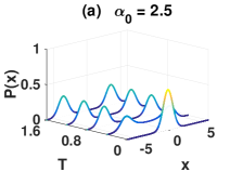
Figure 1: The $x$-quadrature probability distribution (a, c) and $p$-quadrature probability distribution (b, d) as a function of scaled time $T=G^{2}t$ for $\alpha_{0}=2.5$ (a, b) and $\alpha_{0}=10$ (c, d). Here, $\gamma_{1}=0$.

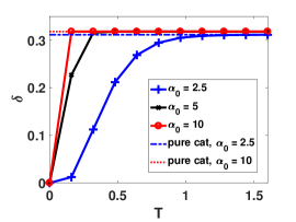
Figure 2: The time evolution of the Wigner negativity $\delta$ for $\alpha_{0}=2.5,\,5,$ and $10$, in terms of the scaled time $T=G^{2}t$. The blue (dashed), black (solid) and red (dashed-dotted) lines correspond to $\alpha_{0}=2.5,\,5,$ and $10$ respectively. The blue dashed horizontal line shows the Wigner negativity for a pure, even cat-state for $\alpha_{0}=2.5$ as calculated from the analytical Wigner function in Eq. (LABEL:eq:Wigner_cat_state). The red dashed-dotted horizontal line corresponds to the same quantity but for $\alpha_{0}=5$ and $10$, which have the same Wigner negativity. The cat-formation time is calculated as the time taken for the Wigner negativity to reach the analytical value associated with the pure cat-state.

These results demonstrate that larger cat-state amplitudes $\alpha_{0}$ have shorter scaled cat-state onset times $T_{\text{cat}}$. We next discuss the cat-formation time $t_{\text{cat}}=T_{\text{cat}}/G^{2}$ for different cat-sizes $\alpha_{0}$ assuming $\gamma_{1}=0$. Recall that a cat-state in the lossless case has an absolute coherent amplitude $|\alpha_{0}|=|\sqrt{\Lambda}/G|$. In order to obtain $|\alpha_{0}|$ of a certain amplitude, one can either fix $G$ and change $\Lambda$ accordingly, or fix $\Lambda$ and change $G$, or change both. If $G$ is fixed while $\Lambda$ is changed to obtain $|\alpha_{0}|$ of a certain amplitude, then $t_{\text{cat}}$ can indeed be shorter for a larger cat-state (Table 1). However, $\Lambda$ scales as $\alpha_{0}^{2}G^{2}$ and this may quickly become impractical for large $\alpha_{0}$.

$\alpha_{0}$	$T_{\text{cat}}$	$t_{\text{cat}}=T_{\text{cat}}/G^{2},$	$t_{\text{cat}}=T_{\text{cat}}\alpha_{0}^{2}/\Lambda$,
		(fixed $G$)	(fixed $\Lambda$)
2.5	$1.75\pm 0.05$	$\left(35.0\pm 1.0\right)\text{$\mu s$}$	$\left(35.0\pm 1.0\right)\text{$\mu s$}$
5.0	$0.45\pm 0.035$	$\left(9.0\pm 0.7\right)\text{$\mu s$}$	$\left(36.0\pm 2.8\right)\text{$\mu s$}$
10.0	$0.14\pm 0.01$	$\left(2.80\pm 0.20\right)\text{$\mu$s}$	$\left(44.8\pm 3.2\right)\text{$\mu s$}$

Table 1: The cat-formation times for fixed $G$ and fixed $\Lambda$. Here $T=G^{2}t$ is the scaled time and $t_{\text{cat}}$ is the real time in seconds. In the third column, we use the estimated value of $G=2.24\times 10^{2}\sqrt{\text{Hz}}$ for the experiment (Leghtas et al., 2015). In the last column, we fix $\Lambda=3.13\times 10^{5}\text{Hz}$.

To get a sense of the timescale in real times, we consider the parameters from the experiment reported in (Leghtas et al., 2015). The nonlinear coupling strength is $\bar{g}/2\pi=225\text{kHz}$, and the Kerr-type interaction strength is $\bar{\chi}/2\pi=4\text{kHz}$. The single signal-photon damping rate is $\gamma_{1}/2\pi=3.98\text{kHz}$, and single pump-photon damping rate $\gamma_{2}/2\pi=3.18\text{MHz}$. In this section, we choose the pump field amplitude to be $\epsilon/2\pi=703\text{kHz}$ such that $|\alpha_{0}|=2.5$, without the Kerr term ($\bar{\chi}=0$), according to Eq. (7). These correspond to parameter values $G=\sqrt{\bar{g}^{2}/\left(2\gamma_{2}\right)}=2.24\times 10^{2}\sqrt{\text{Hz}}$ and $\Lambda=\left|\bar{g}\epsilon\right|/\gamma_{2}=3.13\times 10^{5}\text{Hz}$. In practice, it is better to modify both the parameters $G$ and $\Lambda$ for different $\alpha_{0}$. For the sake of our discussion, however, we consider the case where $\Lambda=3.13\times 10^{5}\text{Hz}$ is fixed and we change $G$ accordingly, where $G$ scales as $\sqrt{\Lambda}/\alpha_{0}$. Hence, $t_{\text{cat}}=T_{\text{cat}}/G^{2}=T_{\text{cat}}\alpha_{0}^{2}/\Lambda$. The $t_{\text{cat}}$ for different cat sizes are shown in Table 1.

IV.2 Single-photon signal damping

Next, we include the effect of the signal damping ($\gamma_{1}\neq 0$). Apart from the time of evolution, the master equation Eq. (20) has two free parameters $\alpha_{0}$ and $g$, which is the effective ratio of the two-photon nonlinearity to the signal decay rate. For sufficiently small $g$, cat-states cannot form. As mentioned previously, the cat-size is given by the amplitude $\alpha_{0}=\sqrt{\lambda}/g$, and we fix this for each Figure below. The parameter $g$ is changed in order to find the threshold value of $g$ where interference fringes, and hence a cat-state, emerge. We take $\alpha_{0}=2.5$ to be the minimum value of $\alpha_{0}$ corresponding to a cat-state.

Figures 3, 4 and 5 indicate that $g>1$ is the threshold for the emergence of fringes (and hence of a cat-state), regardless of the amplitude $\alpha_{0}$ of the cat size. For $g>1$, the Figures show the interference fringes to become more pronounced as $g$ increases. For long enough $T$, the fringes vanish, as the system approaches a steady-state. The steady state is not a cat-state, having a positive Wigner function (Reid and Yurke, 1992).

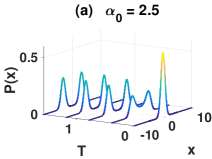
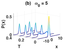
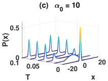
Figure 3: The $x$-quadrature probability distribution as a function of scaled time $T=G^{2}t$ for $g=1$ for various $\alpha_{0}$. The distribution is unchanged for $g=1.5,$ 2.0 and 2.5. We note that $g=G/\sqrt{\gamma_{1}}$.

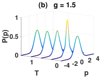
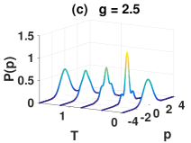
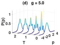
Figure 4: The $p$-quadrature probability distribution as a function of scaled time $T=G^{2}t$ for different values of $g=G/\sqrt{\gamma_{1}}$. Here, $\alpha_{0}=2.5$. For (a), (b), and (c), the time range for $T$ is $0-1.6$. For (d), the time range is $0-2.5$.

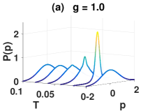
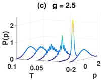
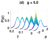
Figure 5: The $p$-quadrature probability distribution as a function of scaled time $T=G^{2}t$ for different values of $g=G/\sqrt{\gamma_{1}}$. Here, $\alpha_{0}=10$.

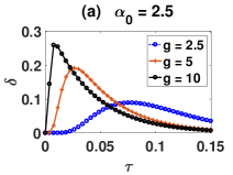
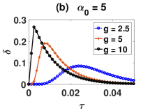
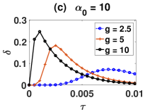
Figure 6: The evolution of Wigner negativity in time $\tau$ (in units of the cavity lifetime $\gamma_{1}^{-1}$) for different values of $\alpha_{0}$. In each plot, the different lines correspond to different $g$ values. The blue, orange and black lines correspond to $g=2.5,\,5$ and $10$ respectively.

It is interesting to know the experimental run-time needed to obtain a cat-like state with the maximal non-classicality. This is quantified by the Wigner negativity. We computed the time evolution of the Wigner negativity. This allows us to estimate the time of formation of a transient state with the largest Wigner negativity, given $\alpha_{0}$ and $g$. In Fig. 6, we present the Wigner negativity results with different $g$’s, for $\alpha_{0}=2.5,\,5$ and $10$ respectively. The results are presented with respect to the time $\tau=\gamma_{1}t=T/g^{2}$ relative to the signal-cavity lifetime. We see first the formation of the cat-state, followed by its decay. Assuming the cavity lifetime is unchanged, for fixed $|\alpha_{0}|$ a larger $g$ implies a quicker formation, but also a quicker decay. Larger cat-sizes $\alpha_{0}$ imply quicker timescales.

We define the cat-state lifetime as the time $\tau$ taken for the Wigner negativity to reduce from the maximum value to $\delta\leq 0.05$. We note that this choice is rather arbitrary and is mainly motivated by the practical consideration that a state with $\delta=0.05$ is too small to be treated as a cat-state or any useful nonclassical state, while at the same time not too small that the numerical simulations remain tractable. A much longer simulation time is needed to reach a state with $\delta=0$, which would be a more natural choice as the cat-state lifetime. The cat-state lifetimes for different values of $g$ and $\alpha_{0}$ are tabulated in Table 2. From the table and Fig. 6, we see that for a fixed $\alpha_{0}$, the cat-states with larger $g$ have a shorter lifetime, even though a larger Wigner negativity can be reached. Also, for fixed $g$, the smaller cat-states have a longer lifetime.

$g$	$T$			$\tau$
	$\alpha_{0}=2.5$	$\alpha_{0}=5$	$\alpha_{0}=10$	$\alpha_{0}=2.5$	$\alpha_{0}=5$	$\alpha_{0}=10$
$2.5$	$0.8206$	$0.2344$	$0.0625$	$0.1313$	$0.0375$	$0.0100$
$5$	$2.250$	$0.5950$	$0.1625$	$0.0900$	$0.0238$	$0.0065$
10	$7.880$	$2.000$	$0.50$	$0.0788$	$0.0200$	$0.0050$

Table 2: The cat-state lifetimes for different $g$ and $\alpha_{0}$ values as given in units of the signal cavity decay time, $\tau=\gamma_{1}t$. Here, $T=G^{2}t$. The cat-state lifetime is defined as the time taken for the Wigner negativity to reach $\delta\leq 0.05$.

Figure 7 shows the photon-number probability distribution at different times, evolving from the vacuum state. The system evolves from a vacuum state into an even cat-state (5). The single-photon loss, however, will cause decoherence and the state evolves into a classical mixture of even and odd cat-states. The time-step errors for the results in Fig. 7 are negligible. The photon number probability distribution at dimensionless time $\tau=0.0150$ centered around $n=100$, which agrees well with the steady state prediction $\left|\alpha\right|^{2}=\lambda/g^{2}=100$. This distribution resembles a Poissonian distribution, as expected for a coherent state.

The Wigner functions at different times are computed according to Eq. (38) and the results are presented in Fig. 8. The function around the origin admits negative values which demonstrates the nonclassical nature of the cat-state.

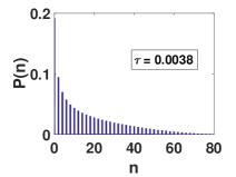
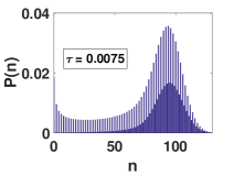
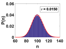
Figure 7: The photon number probability distribution at different times. Here $g=2.5$ and $\alpha_{0}=10$. A state that only allows even photon numbers eventually settles into a state that has a Poissonian distribution. This can be seen in the plot at time $\tau=0.015$, where a Poissonian distribution with a mean photon number of $100$ is fitted in red.

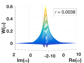
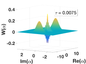
Figure 8: The Wigner function at different times. The parameters are $g=2.5$ and $\alpha_{0}=10$.

V Detuning

We now briefly consider the effect of a detuning ($\omega_{1}-\omega_{p}/2$) between the signal mode and the external field frequency. Under conditions of detuning, the system can display bistability in the intensity of the signal mode as a function of the external driving intensity, which is manifested as a hysteresis cycle (Lugiato et al., 1988; Fabre et al., 1990). The system can also display self pulsing where the outputs give oscillations in their intensities (Lugiato et al., 1988; Fabre et al., 1990). These behaviors can, in turn, affect other quantum properties such as the squeezing amplitudes. A full semiclassical analysis is given in Sun et al. (Sun et al., 2019a).

Here, we investigate the effect of detuning on the transient cat-state. In this work, we consider only the detuning $\Delta=(\omega_{1}-\omega_{p}/2)/\gamma_{1}$ of the signal mode, and only the regime where $\Delta\leq\lambda$ in which case the steady-state semiclassical solution has two stable values (Sun et al., 2019a). We ignore thermal noise and select $\chi=0$.

The Wigner negativity and purity calculations given in Fig. 9 reveal no observable differences in the physical states in the cases with and without detuning. To this end, we plot a Wigner function at an instant in time in Fig. 10. This shows that the two mean values of the Gaussian peaks are no longer situated along the real axis, but are rotated and have acquired complex values. The effect of detuning is to rotate the physical state in phase space, as consistent with the steady state analysis given by Sun et al. (Sun et al., 2019a). This explains the apparent reduction in the visibility of the interference fringes as shown in Fig. 11; the $p$-quadrature is not at an optimal angle to observe the interference fringes.

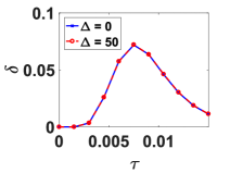
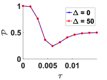
Figure 9: The evolution of (left) the Wigner negativity and (right) the purity for $\Delta=0$ and $\Delta=50$. The parameters are $g=2.5$ and $\lambda/g^{2}=100$. Here $\chi=0$. The results show no difference between the two cases with different detunings.

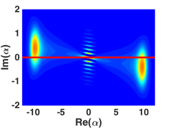
Figure 10: The Wigner function at dimensionless time $\tau=0.0075$. The parameters are $g=2.5$ and $\alpha_{0}=10$. Here $\chi=0$. The detuning is $\Delta=50$. In the presence of detuning $\Delta$, the physical state is rotated in phase space.

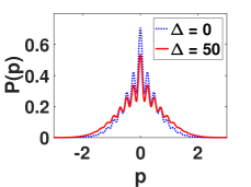
Figure 11: The $p$-quadrature probability distribution at dimensionless time $\tau=0.0067$. The parameters are $g=2.5$ and $\alpha_{0}=10$. Here $\chi=0$. The blue dashed line corresponds to zero detuning and the orange solid line corresponds to $\Delta=50$. Since the detuning rotates the physical state in phase space, the $p$-quadrature is not at an optimal angle to observe the interference fringes. This leads to a reduction in fringe visibility. The Wigner negativity and purity are unaltered from the zero-detuning case.

VI Degenerate parametric oscillation with the anharmonic Kerr interaction

A proposal to generate cat-states with a Kerr interaction is put forward by Yurke and Stoler (Yurke and Stoler, 1986, 1988). They showed that a coherent state can evolve into a multi-component cat-state. Depending on the interaction time, a two-component cat-state can also be created. The mechanism of cat-state creation in a Kerr interaction originates from the fact that the phase acquired by the state is photon-number dependent. This means that this method of creating a cat-state is hard to achieve in the presence of single-photon losses. However, the Yurke and Stoler proposal has been realized in a superconducting circuit experiment (Kirchmair et al., 2013), where the Kerr nonlinearity is larger than $30$ times the single-photon decay rate. Drummond and Walls (Drummond and Walls, 1980) have provided an exact steady-state solution to a driven, dissipative system with a Kerr interaction at zero temperature, which gives quantum predictions that are different from those of a semiclassical analysis.

The combined Kerr and parametric case was studied recently (Sun et al., 2019a, b). These authors gave a derivation of the adiabatic master equation and both semiclassical and exact steady-state solutions. The semiclassical solutions have bistable regimes. There are also tristable regimes, with detunings included. Here, we assume there are no detunings and ignore thermal noise. In this case, the main effect of the additional Kerr nonlinearities is to change the nature of the Schrödinger cat solutions.

Below, we will give more detail by solving the master equation using a particular choice of scaled variables. The master equation including the Kerr nonlinearity is given by

$$\frac{\partial}{\partial t}\rho =\frac{\Lambda}{2}\left[a^{\dagger 2}-a^{2},\rho\right]+\gamma_{1}\left(2a\rho a^{\dagger}-a^{\dagger}a\rho-\rho a^{\dagger}a\right)$$

$$-i\frac{\bar{\chi}}{2}\left[a^{\dagger 2}a^{2},\rho\right]+\frac{1}{2}G^{2}\left(2a^{2}\rho a^{\dagger 2}-a^{\dagger 2}a^{2}\rho-\rho a^{\dagger 2}a^{2}\right)\,$$

where $G=\sqrt{\bar{g}^{2}/\left(2\gamma_{2}\right)}$ and $\Lambda=\left|\bar{g}\epsilon\right|/\gamma_{2}$ as defined previously. We consider $\sqrt{G^{4}+\bar{\chi}^{2}}=G^{2}\sqrt{\left(1+\bar{\chi}^{2}/G^{4}\right)}$ which defines a dimensionless time $\mathcal{T}=\sqrt{G^{4}+\bar{\chi}^{2}}t$. The master equation is then

$$\frac{\partial}{\partial\mathcal{T}}\rho =\!\frac{\Lambda}{2\sqrt{G^{4}+\bar{\chi}^{2}}}\left[a^{\dagger 2}\!-\!a^{2},\rho\right]\!-\!\frac{i\bar{\chi}}{2G^{2}\sqrt{1+\frac{\bar{\chi}^{2}}{G^{4}}}}\left[a^{\dagger 2}a^{2},\rho\right]$$

$$+\frac{\gamma_{1}}{G^{2}\sqrt{1+\frac{\bar{\chi}^{2}}{G^{4}}}}\left(2a\rho a^{\dagger}-a^{\dagger}a\rho-\rho a^{\dagger}a\right)$$

$$+\frac{1}{2}\frac{1}{\sqrt{1+\frac{\bar{\chi}^{2}}{G^{4}}}}\left(2a^{2}\rho a^{\dagger 2}-a^{\dagger 2}a^{2}\rho-\rho a^{\dagger 2}a^{2}\right)\,.$$ (22)

The steady state in the presence of Kerr nonlinearity has a coherent amplitude $\alpha_{0}$ given by (13), with an absolute value $\left|\alpha_{0}\right|=\sqrt{\lambda/\sqrt{g^{4}+\chi^{\prime 2}}}\equiv\sqrt{\Lambda/G^{2}\sqrt{\left(1+\chi^{2}\right)}}$ where $\chi\equiv\bar{\chi}/G^{2}=\chi^{\prime}/g^{2}$. With this choice of scaling factor, the master equation above can be expressed in terms of $\alpha_{0}$, $g$, and $\chi$ as follows:

$$\frac{\partial}{\partial\mathcal{T}}\rho =\frac{1}{2}\left|\alpha_{0}\right|^{2}\left[a^{\dagger 2}-a^{2},\rho\right]-\frac{i}{2}\frac{\chi}{\sqrt{1+\chi^{2}}}\left[a^{\dagger 2}a^{2},\rho\right]$$

$$+\frac{1}{g^{2}\sqrt{1+\chi^{2}}}\left(2a\rho a^{\dagger}-a^{\dagger}a\rho-\rho a^{\dagger}a\right)$$

$$+\frac{1}{2}\frac{1}{\sqrt{1+\chi^{2}}}\left(2a^{2}\rho a^{\dagger 2}-a^{\dagger 2}a^{2}\rho-\rho a^{\dagger 2}a^{2}\right)\,.$$ (23)

In the lossless case ($\gamma_{1}=0$, $g\rightarrow\infty$), the third term does not contribute.

VI.1 No single-photon signal damping

To study the behavior, we first examine the case with no signal damping, corresponding to $\gamma_{1}=0$ (the third term in the master equation is zero). From (23), we see that the free parameters in this case are the coherent amplitude $\left|\alpha_{0}\right|,\,g$ and $\chi\equiv\bar{\chi}/G^{2}=\chi^{\prime}/g^{2}$. We fix $\left|\alpha_{0}\right|$ while changing $\chi$. To keep $\alpha_{0}$ constant for large $r$, we assume a sufficiently large driving field, $\Lambda$ or $\lambda$. Detunings are assumed zero.

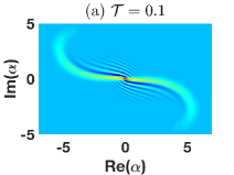
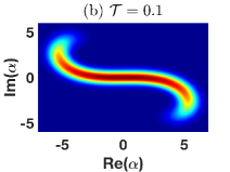
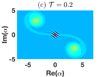
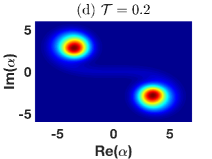
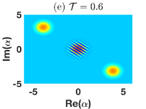
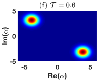
Figure 12: The evolution of the Wigner function (a, c, e) and Q function (b, d, f) with no single-photon damping. In this lossless case, the free parameters determining the dynamics Eq. (23) are $\chi$ and $\left|\alpha_{0}\right|$. Here, $\chi=5$ and $|\alpha_{0}|=5$.

In Fig. 12, we plot the evolution of the Wigner and Q functions for $|\alpha_{0}|=5$ with $\chi=5$. These phase space distributions show the dynamics of the system under the presence of Kerr interaction. Starting with an initial vacuum state, the state quickly turns into a squeezed state with a curved distribution in the phase space distributions due to the large Kerr effect, as shown in Fig. 12 (a) and (b). Some time later, we observe the build up of two Gaussian peaks that correspond to the complex amplitudes with opposite phases as predicted in Eq. (13). Finally, the system reaches a steady state, as shown in Fig. 12 (e) and (f), where the two Gaussian peaks are fully separated. In particular, in the Wigner distribution of Fig. 12 (e), negative values around the origin suggests the presence of cat-states, which is confirmed by computing the corresponding Wigner negativities and compared with the analytical Wigner negativity value of a cat-state as given in Eq. (LABEL:eq:Wigner_cat_state).

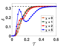
Figure 13: The evolution of the Wigner negativity with different $\chi$ ratios for $\left|\alpha_{0}\right|=5$, in the lossless case $\gamma_{1}=0$. By comparing the numerical Wigner negativity with the analytical Wigner negativity (black dashed horizontal line) for a Wigner function in Eq. (LABEL:eq:Wigner_cat_state), the cat formation time is determined when the numerical value agrees with the analytical value to four significant figures.

The evolution of the Wigner negativity for $|\alpha_{0}|=5$, for different values of $\chi$ is presented in Fig. 13. For $\chi=1$, the Wigner negativity time evolution is similar to that of the case without Kerr interaction. The Wigner negativity increases until reaching a value corresponding to a cat-state. For larger $\chi$, however, the dynamics is markedly different; the negativity rises steadily initially, reaching a peak before decreasing and increasing again until the value reaches the negativity corresponding to that of a cat-state.

An understanding of this dynamics for large $\chi$ can be obtained from the corresponding Wigner function time evolution in Fig. 12. In the earlier stage of the dynamics, the Kerr term dominates the parametric gain term for large $\chi$. The large contribution from the Kerr effect produces a nonclassical state; the larger the Kerr strength, the larger the peak Wigner negativity. As the two Gaussian peaks with the same amplitude but opposite phases are building, the Wigner negativity value decreases, before increasing again due to the formation of a cat-state as the system approaches the steady state. We note that a cat-state corresponds to the case where the Wigner function has two fully separated Gaussian peaks with the presence of interference fringes around the origin.

We also plotted the evolution of the rotated quadrature probability distributions $P\left(x_{\phi}\right)$ and $P\left(x_{\phi+\pi/2}\right)$, where the angle $\phi$ is determined from the predicted complex amplitude $\alpha_{0}=|\alpha_{0}|e^{i\phi}$ as given in Eq. (13). The results are plotted in Figs. 14 and 15 for $|\alpha_{0}|=5$ and $|\alpha_{0}|=10$ respectively. In each figure, the rotated quadrature probability distributions for different $\chi$ values are also presented. For larger $\chi$, it takes a similar dimensionless time $\mathcal{T}$ for the quadrature probability distribution to reach the one that corresponds to a cat-state, which implies a shorter real time.

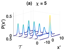
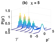
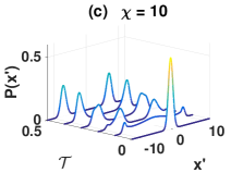
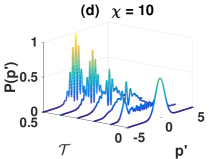
Figure 14: The evolution of quadrature probability distributions $x^{\prime}=x_{\phi}$ and $p^{\prime}=x_{\phi+\pi/2}$ respectively, for (a,b) $\chi=5$ and (c,d) $\chi=10$. Here, $|\alpha_{0}|=5$ and the angle $\phi$ is determined from the predicted complex amplitude $\alpha_{0}=|\alpha_{0}|e^{i\phi}$ as given in Eq. (13).

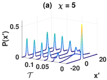
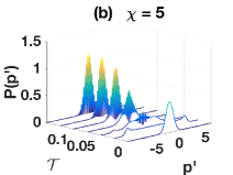
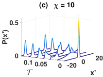
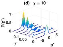
Figure 15: The evolution of quadrature probability distributions $x^{\prime}=x_{\phi}$ and $p^{\prime}=x_{\phi+\pi/2}$ respectively, for (a,b) $\chi=5$ and (c,d) $\chi=10$. Here, $|\alpha_{0}|=10$ and the angle $\phi$ is determined from the predicted complex amplitude $\alpha_{0}=|\alpha_{0}|e^{i\phi}$ as given in Eq. (13). The time range for all plots is $0-0.15$.

The cat-formation times for different $\chi$ and $|\alpha_{0}|$ values, in both the dimensionless time $\mathcal{T}_{\text{cat}}$ and real time $t_{\text{cat}}=\mathcal{T}_{\text{cat}}/\left(G^{2}\sqrt{1+\chi^{2}}\right)$, are presented in Table 3 using the value of $G=2.24\times 10^{2}\sqrt{\text{Hz}}$ as taken from the parameters of the experiment of Leghtas et al. (2015) (refer Section IV.1). The cat-formation time is determined by comparing the numerical Wigner negativity with that of a pure cat-state Wigner function in Eq. (LABEL:eq:Wigner_cat_state). From the table, we see that for a cat-state of fixed amplitude, a similar nonlinearity $\chi$ has a larger $\mathcal{T}_{\text{cat}}$, in agreement with the observations in Figs. 14 and 15. Also from the table, a longer $\mathcal{T}_{\text{cat}}$ corresponds to a shorter $t_{\text{cat}}$. Thus, a larger Kerr interaction speeds up the cat-formation time.

$\chi$	$\mathcal{T}_{\text{cat}}$		$t_{\text{cat}}=\mathcal{T}_{\text{cat}}/\left(G^{2}\sqrt{1+\chi^{2}}\right)$ ($\mu s$)
	$\left|\alpha_{0}\right|=5$	$\left|\alpha_{0}\right|=10$	$\left|\alpha_{0}\right|=5$	$\left|\alpha_{0}\right|=10$
$0$	$0.40\pm 0.02$	$0.125\pm 0.005$	$8.00\pm 0.40$	$2.50\pm 0.10$
$1$	$0.44\pm 0.02$	$0.130\pm 0.005$	$6.22\pm 0.28$	$1.84\pm 0.07$
$2$	$0.52\pm 0.02$	$0.135\pm 0.005$	$4.65\pm 0.18$	$1.21\pm 0.04$
$5$	$0.74\pm 0.02$	$0.20\pm 0.005$	$2.90\pm 0.08$	$0.78\pm 0.02$

Table 3: The cat-formation times for different values of the nonlinear parameter $\chi$ and $\left|\alpha_{0}\right|$. The parameter $G=2.24\times 10^{2}\sqrt{\text{Hz}}$ is used to convert the dimensionless time $\mathcal{T}_{\text{cat}}$ to the real time $t_{\text{cat}}$.

VI.2 Single-photon signal damping

Now we focus on the case where $\gamma_{1}\neq 0$ i.e. $g$ is finite. We examine the transient behavior of the signal field assuming the initial state is the vacuum state. The free parameters in this case are the coherent amplitude $\left|\alpha_{0}\right|,\,g$ and $\chi$, as well as the scaled time $\mathcal{T}=\left(g^{2}\sqrt{1+\chi^{2}}\right)t$.

In the presence of single-photon damping, an ideal pure cat-state cannot be formed even as a transient state. This is true without the Kerr interaction, but becomes more noticeable in the solutions we give for nonzero $\chi$. Rather, in an optimal situation, a cat-like state is formed where two peaks are fully separated and interference fringes are present around the origin. Here, we define the cat lifetime as the time taken for the Wigner negativity to reach $\delta\leq 0.05$, provided the quadrature distributions are initially consistent with a cat-state, being two-peaked for $x^{\prime}$ and with fringes for $p^{\prime}$.

It is reported that a cat-like state has been observed in the experiment of Leghtas et al. (Leghtas et al., 2015). In the following, we carry out the numerical simulation of the experiment using the published experimental parameters where $g=1.41$, $\chi^{\prime}=1.01$, giving $\chi=0.5$ and an estimated coherent amplitude $\left|\alpha_{0}\right|=2$. The numerical results are shown in Fig. 16 where the time evolution of the quadrature probability distributions and the Wigner negativity are plotted. We see from Fig. 16 (top left) that the coherent peaks in $x^{\prime}$ with opposite phases are never fully separated for $|\alpha_{0}|=2$. The largest Wigner negativity value in the simulation, located around dimensionless time $\mathcal{T}=0.5$ is small ($\sim 0.025$) and this is reflected by the absence of observable interference fringes in the quadrature probability distribution in Fig. 16 (top right). This supports that, while a nonclassical state is produced in the experiment, the state is not a mesoscopic cat-state: The coherent peaks are not fully separated and the non-classicality of the state as quantified by the Wigner negativity is weak.

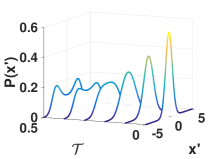
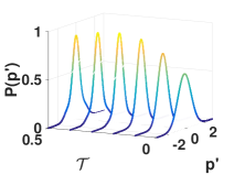
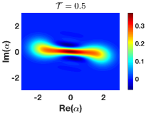
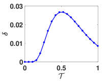
Figure 16: The quadrature probability distributions as a function of time (top left and right). The bottom left figure shows the Wigner function at $\mathcal{T}=0.5$, which has the largest Wigner negativity $\delta$ as given in the bottom right plot. Here, the experimental parameters (Leghtas et al., 2015) are $g=1.41$, $\chi^{\prime}=1.01$, giving $\chi=0.5$ and an estimated coherent amplitude $\left|\alpha_{0}\right|=2$.

In Table 4, we evaluate the cat-lifetime as defined in the previous section, by evaluating the time taken for a cat-state to decay to a Wigner negativity smaller than $0.05$. For the parameters of the experiment, we note again that for $|\alpha_{0}|=2$, the steady state corresponds to two peaks in $x^{\prime}$ that are not fully separated. From the table, for $g\leq 1.5$, the Wigner negativity does not exceed $0.05$ and is too small (when compared to a pure cat-state with amplitude $|\alpha_{0}|=2$, which has a Wigner negativity of $0.2937$ as predicted by Eq. LABEL:eq:Wigner_cat_state) to be considered a cat-state at any point of the simulation. True cat-states are generated for higher $g$, however. Next, we investigate the non-classicality of transient cat-states with larger coherent amplitudes and Kerr strengths.

$\chi$	$\mathcal{T}_{\text{life}}$			$t_{\text{life}}=\mathcal{T}_{\text{life}}/\left(\text{$\gamma$}g^{2}\sqrt{1+\chi^{2}}\right)$ $(\mu s)$
	$g=1$	$g=1.5$	$g=2.5$	$g=2.5$
$0.5$	$0$	$0$	$1.225$	$7.01$
$1.0$	$0$	$0$	$1.375$	$6.22$

Table 4: The cat-like state lifetime for different $\chi$ and $g$ values, for $|\alpha_{0}|=2$. For comparison, the experimental parameters of Leghtas et al. (Leghtas et al., 2015) are $g=1.41$, $\chi=0.5$ and $\gamma=2\pi\times 3.98\text{kHz}$.

To study the effect of single-photon damping, we compute the time evolution of the quadrature phase amplitude distributions and Wigner negativity, varying $g$ for different values of $\chi$ and $|\alpha_{0}|$. Recall in Section VI.1 with no signal single-photon loss that a large Kerr interaction speeds up the cat-formation time. As a cat-state is highly nonclassical, the system parameters that lead to earlier cat formation might also lead to a quicker decay/decrease in the Wigner negativity and the corresponding cat-state lifetime. This is confirmed by Table 4 for the experimental parameters of (Leghtas et al., 2015).

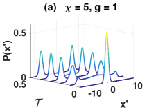
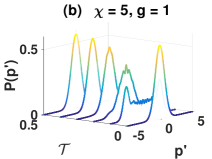
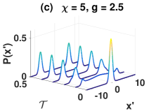
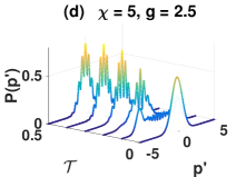
Figure 17: The evolution of quadrature probability distributions $x^{\prime}=x_{\phi}$ and $p^{\prime}=x_{\phi+\pi/2}$ respectively, in the presence of single-photon damping. The angle $\phi$ is determined from the predicted complex amplitude $\alpha_{0}=|\alpha_{0}|e^{i\phi}$ as given in Eq. (13). Here, $\chi=5$, $|\alpha_{0}|=5$ with $g=1$ and $2.5$.

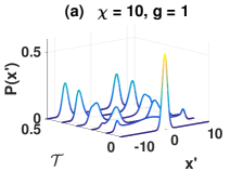
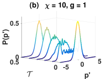
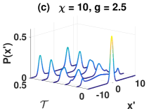
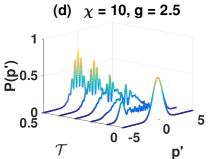
Figure 18: Description as for Figure 17. Here, $\chi=10$, $|\alpha_{0}|=5$ with $g=1$ and $2.5$.

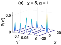
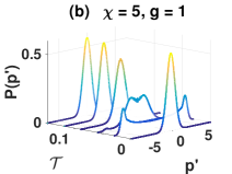
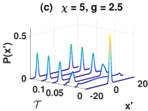
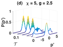
Figure 19: Description as for Figure 17. Here $|\alpha_{0}|=10$. The time range for all plots is $0-0.15$.

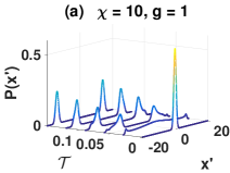
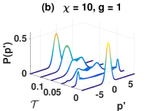
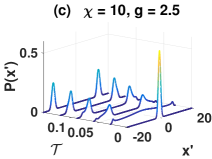
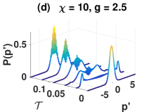
Figure 20: Description as for Figure 18. Here $|\alpha_{0}|=10$. The time range for all plots is $0-0.15$.

Another question to be answered is whether the presence of a Kerr effect changes the threshold of $g$ required for a cat-state. We find that $g>1$ is still required for the generation of a cat state. The results for different $\chi$ and $|\alpha_{0}|$ are presented in Figs. 17, 18, 19, and 20. Figs. 17 and 18 show the time evolution of the quadrature probability distributions for $|\alpha_{0}|=5$ with $\chi=5$ and $\chi=10$, respectively. The same quantities are plotted in Figs. 19 and 20 for $|\alpha_{0}|=10$. The emergence of interference fringes corresponds to $g\geq 1$ even in the presence of large Kerr strength. These results are confirmed by the time evolution of the Wigner negativity as presented in Figs. 21 and 22. When $g$ is large enough to produce cat-like states, these figures also show larger Wigner negativities with larger $\chi$ for the same $\alpha_{0}$ and $g$ values.

We emphasize the need to compute several cat-state signatures and caution the use of any single signature alone to interpret the nonclassicality of the physical state. For instance, the Wigner negativity is not sufficient to infer the presence of a cat-state. The peak values of Wigner negativity observed in Figs. 21 and 22 for $\chi=5$ do not correspond to cat-states, despite the large negativity values. These large negativities correspond to nonclassical states that arise due to the large Kerr interaction term, before the formation of cat-states. As previously discussed, a cat-state is formed when two well-separated peaks in $P(x^{\prime})$ are observed and when interference fringes in the corresponding $P(p^{\prime})$ distribution exist. This can be inferred from the quadrature probability distributions or the Wigner function itself, but not directly from the Wigner negativity.

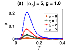
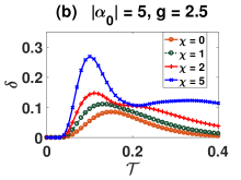
Figure 21: The evolution of the Wigner negativity with different $\chi$ values for (a) $g=1$ and (b) $g=2.5$. In both cases, $\left|\alpha_{0}\right|=5$. Note that a peak in the Wigner negativity does not imply the formation of a cat-state (see main text). The verification of a cat-state can only be drawn in conjunction with other cat-state signatures such as in Fig. 17.

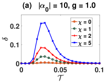
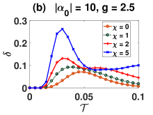
Figure 22: The evolution of the Wigner negativity with different $\chi$ values for (a) $g=1$ and (b) $g=2.5$. In both cases, $\left|\alpha_{0}\right|=10$.

We also see that with a finite $g$ (signal losses), as for the earlier case without nonlinearity, the cat-state eventually decoheres to a mixed state. More loss (lower $g$) gives a faster decay, for fixed nonlinearity $\chi$ and $\alpha_{0}$. This is quantified in the Table 5 which evaluates the Wigner negativity. Also from the table, we see that for fixed $g$ and $\alpha_{0}$, the cat-state decoheres faster for the larger $\chi$ value given here.

(a) $\chi$ $\mathcal{T}_{\text{life}}$ $t_{\text{life}}=\mathcal{T}_{\text{life}}/\left(\gamma g^{2}\sqrt{1+\chi^{2}}\right)$ $(\mu s)$ $g=1$ $g=1.5$ $g=2.5$ $g=2.5$ 5 $0$ $0$ $0.68$ $0.85$ 10 $0$ $0$ $1.25$ $0.80$

(b) $\chi$ $\mathcal{T}_{\text{life}}$ $t_{\text{life}}=\mathcal{T}_{\text{life}}/\left(\gamma g^{2}\sqrt{1+\chi^{2}}\right)$ $(\mu s)$ $g=1$ $g=1.5$ $g=2.5$ $g=2.5$ 5 $0$ 0 $0.177$ $0.222$ 10 $0$ 0 $0.324$ $0.206$

Table 5: The cat-like state lifetime for different $\chi$ and $g$ values, for (a) $|\alpha_{0}|=5$ and (b) $|\alpha_{0}|=10$. Here, $\gamma=2\pi\times 3.98\text{kHz}$. We comment that for $g=1.5$, the small value of negativity is not associated with well-separated peaks in the distribution of $x^{\prime}$ (Figs. 17, 18, 19, and 20). Hence we do not claim these are cat-states.

VII Large transient cat

In this section, we investigate the feasibility of observing a transient cat state using physical parameters that are achievable in an experiment similar to the superconducting-cavity setup discussed in the previous subsection. The effects of finite temperatures leading to thermal noise are also included. We choose $g=2$ and $\left|\alpha_{0}\right|=20$, which corresponds to a coherent amplitude of $20$. We focus on the quadrature probability distribution as a cat-state signature. In order to achieve $g=2$ in an experiment, either the signal decay rate has to be reduced or the nonlinear coupling strength has to be enhanced, or both.

We computed the evolution of the quadrature probability distributions both with and without the Kerr nonlinear interaction at zero temperature. The results are shown in Figs. 23 and 24. For the nonzero Kerr case, it is the rotated quadrature probability distributions $P\left(x_{\phi}\right)$ and $P\left(x_{\phi+\pi/2}\right)$ that are plotted, where the angle $\phi$ is determined from the predicted complex amplitude $\alpha_{0}=|\alpha_{0}|e^{i\phi}$ as given in Eq. (13). From these figures, the interference fringes appear sooner in the presence of Kerr nonlinear interaction. This observation is confirmed in Fig. 25, where snapshots of these interference fringes in the quadrature probability distributions are presented. We include plots with thermal noise of $N$ thermal photons present in the reservoir. Even though we assume an initial vacuum state, as in previous calculations, the reservoir thermal noise causes a decoherence that destroys the cat-state.

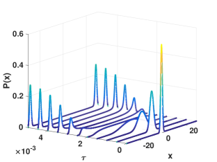
Figure 23: The evolution of the quadrature probability distributions in scaled time $\tau=\gamma t$. Here, the parameters are $g=2$, $\left|\alpha_{0}\right|=20$ and $\chi=0$ at zero temperature. The time range for all plots is $0-0.005$.

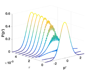
Figure 24: The evolution, in scaled time $\tau=\gamma t$, of the rotated quadrature probability distributions $x^{\prime}=x_{\phi}$ and $p^{\prime}=x_{\phi+\pi/2}$ respectively. The angle $\phi$ is determined from the predicted complex amplitude $\alpha_{0}=|\alpha_{0}|e^{i\phi}$ as given in Eq. (13). Here, the parameters are $g=2$, $\left|\alpha_{0}\right|=20$ and $\chi=5$ at zero temperature. The time range for all plots is $0-0.005$.

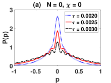
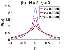
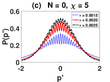
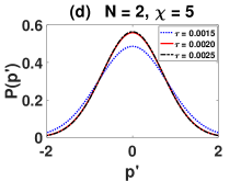
Figure 25: Snapshots of the quadrature probability distribution showing the interference fringes for the case (top) without and (lower) with Kerr nonlinear interaction. Here, the parameters $g=2$, $\left|\alpha_{0}\right|=20$ and $p^{\prime}$ are the same as in Fig. 24. The case with thermal noise is characterized by the mean thermal occupation number $N$.

The decoherence mechanism is known for this system. The single-photon damping process switches the state between even and odd cat-states with probabilities that scale with the single-photon damping rate, and are further enhanced by the thermal noise. Eventually, the system reaches a steady state where it is a mixture of the even and odd cat-states. A detailed mathematical analysis of the decoherence process discussed here can be found in Ref. (Carmichael, 2009).

It is appropriate to discuss a few points on the factors that might limit the achievable cat-state amplitude. In the case without detuning and Kerr-nonlinearity, the coherent state in the superposition has an amplitude of $\sqrt{\lambda}/g$. Assuming all other cat-state destroying parameters ($\gamma_{1},\,N$) remain the same, for larger $g$, an even larger $\lambda$ is needed to obtain the same cat-state amplitude, which can be hard to achieve.

There are also difficulties from the point of view of calculation. This work uses the number-state basis expansion of the density operator and the cutoff number scales roughly with the coherent amplitude as $\left|\alpha_{0}\right|^{2}+\left|\alpha_{0}\right|$, where $\alpha_{0}$ is the coherent amplitude of the state. The super-operator that dictates the time evolution of the density operator has a size of $n_{c}^{2}\times n_{c}^{2}$, where $n_{c}$ is the cutoff number, and this quickly becomes problematic even if the super-operator is represented as a sparse matrix. Also, the cat-state signatures such as the Wigner function and its negativity are almost not computable even with quadruple-precision computation. Other methods such as the positive-P phase space representation are available and are more suited for computations in this regime. However, more sophisticated techniques (Deuar and Drummond, 2002) in phase space methods have to be employed when the quantum noise is large ($g>1$). Even though the Q-function is always positive and does not signify nonclassicality when the state is a mixed state, it nevertheless has the merit that its numerical computation is stable. Together with other cat-state signatures, the Q-function can still serve as a good nonclassicality indicator. Other cat-state signatures such as the quadrature probability distributions can be computed to a very large photon number cutoff (much larger than $500$, which is needed for cat amplitude $\alpha_{0}>20$) though efficient algorithms such as the Clenshaw algorithm for evaluating sums involving orthogonal polynomials are required.

VIII conclusion

It is known that a Schrödinger cat state is formed as the steady state of a degenerate parametric oscillator, in the limit where single-photon damping is zero and the initial condition is a vacuum state (Gilles et al., 1994; Hach III and Gerry, 1994). In the same limit, under an additional nonlinear Kerr interaction, the corresponding steady state is also a cat-state (Sun et al., 2019b). It is illuminating to study the dynamics in the lossless case, as the interplay between the different nonlinear interactions affects the cat-formation time, providing a better understanding of the physics involved in the formation of a cat-state. In Sections IV.A, and VI.A, we have examined this limit, showing in Section VI.A how the Kerr nonlinearity can enhance the formation of the cat-state. In particular, we examine the effect of the Kerr nonlinearity on the threshold value of $g$, and illustrate how the formation time and lifetime of the cat-state is affected by the Kerr nonlinearity in the zero temperature limit.

In practice, the cavity single-photon damping is very important. This causes decoherence and eventually destroys the cat-state, as known from previous exact steady-state results. In Section IV.B, we analyze the effect of this using a parameter $g$ which gives the strength of parametric nonlinearity relative to the single-photon signal decay rate. A threshold value of $g$ is necessary for a cat-state to form. When $g$ is large enough to form a cat-state, we find that a larger $g$ will lead to a physical state with a larger Wigner negativity, implying the formation of a more nonclassical state. However, the more nonclassical the state is, the shorter is its lifetime.

We also examine the effects of detuning $\Delta$, in Section V. With all other DPO parameters being equal, the presence of detuning rotates the physical state in phase space, and does not affect the Wigner negativity and purity of the state throughout the dynamics of the system. The Kerr nonlinearity also rotates the state in phase space. Unlike detuning, however, the Kerr interaction also changes the nonclassicality of the state. This is examined in Section VI.

For large $\chi$, where the Kerr interaction strength is larger than the parametric gain $g$, the Kerr term dominates the dynamics of the system in the early stage. The larger the Kerr strength, the larger the value of the corresponding Wigner negativity. As the two stable states with equal amplitudes but opposite phases are gradually formed due to the parametric term, the Wigner negativity decreases, before increasing again as the cat-state is fully reached. A cat-state must have two well-separated peaks along the phase space axis where the two amplitudes lie, and hence the dynamical picture given here is only clear when different cat-state signatures are computed and compared. The Wigner negativity alone does not provide conclusive evidence of a cat-state. Two distinct probability peaks and the presence of interference fringes in the orthogonal quadrature are also necessary. This can be seen in the quadrature probability distribution and Wigner function, which confirms the macroscopic coherence between the two peaks.

With this physical picture established, we carried out a numerical simulation in Section VI.B of a recent experiment of Leghtas et al. (Leghtas et al., 2015). While a nonclassical state is produced, in agreement with experimental measurements of Wigner negativity, it does not appear to be a fully mesoscopic cat-state. The coherent peaks are not fully separated and the nonclassicality is relatively weak. This is indicated by absence of significant interference fringes in the quadrature probability distribution and relatively small Wigner negativities. We nevertheless agree that this was an important experimental step towards demonstrating a fully developed mesoscopic superposition of two well-separated coherent states.

By exploring the parameter space, we find that $g>1$ is still required for the cat-state generation, irrespective of the Kerr interaction strength $\chi$. When $g$ is large enough for cat formation, for a fixed coherent amplitude $|\alpha_{0}|$, a larger $\chi$ takes a shorter time to form a cat-state and also has a larger Wigner negativity. However, it has a shorter lifetime, as defined by the Wigner negativity in Section IV.

The ability to compute the time evolution of the physical state allows us to estimate the lifetime of a cat-state including thermal noise. An example is given for large $|\alpha_{0}|$ in Section VII. To obtain a large cat amplitude in the presence of thermal noise, which tends to destroy the coherence of the cat-state, a large value of $g$ is necessary. Alternatively, a system that has a lower temperature or lower cavity decay rate is required. The engineering of the reservoir, for instance, with squeezed states, as a means of noise reduction is also possible and will be explored in a future publication.

Appendix

Appendix A Cat-state and signatures

Here we summarize the cat-state signatures that verify the presence of cat-states in the system. We focus on the simplest example, in which we use these signatures to distinguish the difference between a cat-state

$$|\psi_{\text{cat}}\rangle =\mathcal{N}_{\theta}\left(|\alpha_{0}\rangle+e^{i\theta}|-\alpha_{0}\rangle\right)\,$$ (24)

which is a superposition of two coherent states $|\pm\alpha_{0}\rangle$ well-separated in phase space ($\mathcal{N}_{\theta}$ is a normalization constant and $\theta$ a phase), and an arbitrary mixture of the two coherent states given by the density operator

$$\rho_{\text{mix}}=P_{+}|\alpha_{0}\rangle\langle\alpha_{0}|+P_{-}|-\alpha_{0}\rangle\langle-\alpha_{0}|\,,$$ (25)

where $P_{\pm}$ are probabilities and $P_{+}+P_{-}=1$.

The objective is to confirm that the system is not in the coherent state mixture (25). Thus, if we consider systems confined to be in a mixture of the two coherent states, or in a mixture of superpositions of the two coherent states, the exclusion of the mixture (25) implies some type of cat-like state, although not necessarily a pure cat-state. For definiteness, we also require that a cat-state have clear operational signatures of fringes or Wigner negativity, as we explain below.

Realizing it is possible the system may be in a state of reduced purity, the general confined density operator can be written with off-diagonal terms as

$$\rho = P_{11}|\alpha_{0}\rangle\langle\alpha_{0}|+P_{22}|-\alpha_{0}\rangle\langle-\alpha_{0}|$$ (26)

$$+P_{12}|\alpha_{0}\rangle\langle-\alpha_{0}|+P_{21}|-\alpha_{0}\rangle\langle\alpha_{0}|$$

This state can also be written in terms of the odd and even cat-states as

$$\rho =p_{++}|\psi_{\text{even}}\rangle\langle\psi_{\text{even}}|+p_{--}|\psi_{\text{odd}}\rangle\langle\psi_{\text{odd}}|$$

$$+p_{+-}|\psi_{\text{even}}\rangle\langle\psi_{\text{odd}}|+p_{-+}|\psi_{\text{odd}}\rangle\langle\psi_{\text{even}}|\,$$ (27)

We note that these “impure cat-states” may or may not give a result that, for example, has interference fringes. As a result, it is an open question whether such intermediate states are identifiable by any of the criteria in common use. It is also possible that the system cannot be represented in terms of the two coherent states alone, in which case a broader class of mixtures needs to be excluded. Alternative approaches to detecting mesoscopic coherence are discussed elsewhere (Bennett et al., 1996; Terhal and Horodecki, 2000; Brennen, 2003; Cavalcanti and Reid, 2006; Korsbakken et al., 2007; Cavalcanti and Reid, 2008; Fröwis and Dür, 2012; Baumgratz et al., 2014; Sekatski et al., 2014; Fröwis et al., 2015; Oudot et al., 2015; Fröwis et al., 2016; Yadin and Vedral, 2016; Fröwis et al., 2018; Teh et al., 2018) and include those based on uncertainty relations (Cavalcanti and Reid, 2006, 2008; Teh et al., 2018; Reid, 2019).

In this paper, we identify the cat-state using both interference fringes and negativity of the Wigner function. Where the distribution for one quadrature phase amplitude ($X$) shows two well-separated Gaussian peaks corresponding to the two coherent states, the observation of interference fringes in the orthogonal quadrature ($P$) excludes all models of the form of (25). This gives evidence of a significant quantum coherence, which is one type of signature of a Schrödinger cat-state.

However, if the associated Wigner function is observed to be positive, then there exists a joint probability distribution $P(x,p)$ to correctly describe the marginal probability distributions $P(x)$ and $P(p)$ for the results $x$ and $p$ of measurements $X$ and $P$. It is then possible to construct two “elements of reality”, the variables $x$ and $p$, that directly and simultaneously predetermine the results for $X$ and $P$. While these “elements of reality” $x$ and $p$ do not describe quantum states (being simultaneously precisely defined (Reid, 2019)), the system can nonetheless, with respect to these variables, be interpreted as being in one or other of states corresponding to the Gaussian peaks in $X$. This interpretation is not possible for the ideal cat-state (24) which possesses a negative Wigner function. Thus, the observation of interference fringes associated with a negative Wigner function (consistent with that of the state (24)) gives strong evidence of a cat-state.

A.1 Interference fringes in the quadrature probability distribution

One of the earliest proposed cat state signatures is the presence of interference fringes in the quadrature probability distribution (Yurke and Stoler, 1986, 1988). In order to understand the origin of the interference fringes, consider an even cat-state

$$|\psi_{\text{even}}\rangle =\mathcal{N}_{+}\left(|\alpha_{0}\rangle+|-\alpha_{0}\rangle\right)\,$$ (28)

Without losing generality, we assume that $\alpha_{0}$ is real, and that $|\alpha_{0}|$ is large. The $x$-quadrature for this state has two contributions from two well-separated phase points along $x$-axis. The corresponding $x$-quadrature probability distribution has two significant Gaussian distributions centered around these two phase points along the $x$-axis. This gives us justification to assume the system is either a superposition, or a mixture, as in (26).

To exclude the statistical mixture (25), one measures the orthogonal quadrature $p$. For a cat-state (24), the probability amplitudes for these two possible contributions $|\pm\alpha_{0}\rangle$ have to be summed, and hence there will be interference fringes in the $p$-quadrature probability distribution for this cat state. These fringes cannot arise for the system given by the classical mixture (25) which is therefore excluded if fringes are observed. If we consider the coherent-state manifold, with $\alpha_{0}\geq 2.5$ to allow for distinct Gaussian distributions, the onset of fringes implies failure of the mixture (25), so that $P_{12}$ and $P_{21}$ defined by eq. (26) must be nonzero.

More generally, a cat-state may be in a manifold of superposition states spanned by two coherent states $\left\{|\alpha_{0}\rangle,|-\alpha_{0}\rangle\right\}$, where $\alpha_{0}$ is a complex number and these two coherent states can have any phase relation between them. Therefore, we define a general rotated quadrature operator $x_{\theta}=\left(e^{-i\theta}a+e^{i\theta}a^{\dagger}\right)/\sqrt{2}$. The $x_{\theta}$-quadrature probability distribution can be computed from a density operator $\rho$ which is expanded in the number state basis. The probability distribution $P\left(x_{\theta}\right)$ is then

$$\langle x_{\theta}|\rho|x_{\theta}\rangle =\langle x_{\theta}|\left(\sum_{n,m}\rho_{nm}|n\rangle\langle m|\right)|x_{\theta}\rangle$$

$$=\sum_{n,m}\rho_{nm}\langle x_{\theta}|n\rangle\langle m|x_{\theta}\rangle\,,$$ (29)

where

$$\langle x_{\theta}|n\rangle =\frac{e^{-i\theta n}}{\sqrt{2^{n}n!\sqrt{\pi}}}e^{-\frac{x_{\theta}^{2}}{2}}H_{n}\left(x_{\theta}\right)\,.$$ (30)

Here, $H_{n}\left(x\right)$ is the Hermite polynomial. In particular, for $\theta=0$, $x_{\theta=0}=x$ and for $\theta=\pi/2$, $x_{\theta=\pi/2}=p$, and their inner products with a number state are given by

$$\langle x|n\rangle =\frac{1}{\sqrt{2^{n}n!\sqrt{\pi}}}e^{-\frac{x^{2}}{2}}H_{n}\left(x\right)$$ (31)

$$\langle p|n\rangle =\frac{\left(-i\right)^{n}}{\sqrt{2^{n}n!\sqrt{\pi}}}e^{-\frac{p^{2}}{2}}H_{n}\left(p\right)$$ (32)

respectively. For an even cat-state with real-valued coherent amplitudes, $\alpha_{0}$, the $p$-quadrature probability distribution is given by (Yurke and Stoler, 1988; Teh et al., 2018)

$$P\left(p\right) =\frac{1}{\sqrt{\pi}}\mathcal{N}_{+}^{2}\left\{2\text{exp}\left(-p^{2}\right)\left[1+\cos\left(2\sqrt{2}p\alpha_{0}\right)\right]\right\}\,,$$ (33)

For comparison purposes, we plot $P\left(p\right)$ for $\alpha_{0}=5$ in Fig. 26 using Eq. (33).

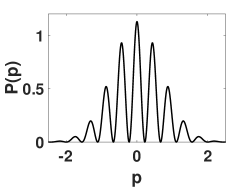
Figure 26: The $p$-quadrature probability distribution for a pure, even cat-state with $\alpha_{0}=5$.

In this work, a number state cutoff of up to $500$ is used. There is a floating point number overflowing issue in the numerical computation of Eqs. (31) and (32), which arises from the evaluation of the Hermite polynomials. This issue is overcome by using a Matlab function (Polkinghorne, 2019) that employs logarithmic manipulation. Moreover, this Matlab function is based on the Clenshaw algorithm (Clenshaw, 1955; Press et al., 2007) that computes orthogonal polynomials more efficiently and accurately (Smith, 1965) than either naively computing the summations involved or other methods using the Hermite polynomials recurrence relation such as the Forsythe method (Forsythe, 1957).

A.2 Photon-number probability distribution

Yet another aspect where the quantum superposition of a cat state is manifested is in the photon-number probability distribution. The even cat-state Eq. (28)

$$|\psi_{\text{even}}\rangle =\mathcal{N_{+}}\left(|\alpha_{0}\rangle+|-\alpha_{0}\rangle\right)$$

$$=\mathcal{N_{+}}e^{-\frac{\left|\alpha_{0}\right|^{2}}{2}}\sum_{n}^{\infty}\frac{1}{\sqrt{n!}}\left[\alpha_{0}^{n}+\left(-\alpha_{0}\right)^{n}\right]|n\rangle\,,$$ (34)

contains an even number of photons. Similarly, an odd cat-state $|\psi_{\text{odd}}\rangle=\mathcal{N_{-}}\left(|\alpha_{0}\rangle-|-\alpha_{0}\rangle\right)$ has an odd number of photons. For a classical mixture of $|\alpha_{0}\rangle$ and $|-\alpha_{0}\rangle$, the photon number probability distribution is nonzero for both even and odd numbers of photons. Hence, assuming we are in the manifold of the superpositions of the two coherent states (or their mixtures), the photon-number probability distribution reveals both the nonclassicality of a cat-state and its phase relation. It is possible that the system is in a superposition of both the even and odd cat-states, and the photon number probability distribution does not distinguish between this state and a classical mixture of the even and odd cat-states. With that, we also computed the purity of the state given by

$$\mathcal{P} {\normalcolor=}\text{Tr}\left(\rho^{2}\right)\,.$$ (35)

A.3 Phase-space distributions

It is also useful to consider phase-space distributions that can determine the entire quantum states, and display quantum features. In particular, we compute the Husimi Q and Wigner functions.

A.3.1 Wigner function and its negativity

The Wigner function gives us the joint probability distribution of the real and imaginary parts of the coherent amplitude of the quantum state, which allows the deduction of the form of a cat state. The Wigner function for a density operator in a Fock state for a finite particle number is given by (Cahill and Glauber, 1969; Pathak and Banerji, 2014)

$$W\left(\alpha,\alpha^{*}\right) =\sum_{n}^{N_{c}}\rho_{nn}X_{nn}+2\text{Re}\left(\sum_{m=1}^{N_{c}}\sum_{n=0}^{m-1}\rho_{nm}X_{nm}\right)\,,$$ (36)

where $n<m$, $\rho_{nm}$ is the matrix element of the density operator $\rho$ and $X_{nm}$ is (Cahill and Glauber, 1969; Pathak and Banerji, 2014)

$$X_{nm} =\frac{2\left(-1\right)^{n}}{\pi}\sqrt{\frac{n!}{m!}}e^{-2\left|\alpha\right|^{2}}\left(2\alpha\right)^{m-n}L_{n}^{m-n}\left(4\left|\alpha\right|^{2}\right)\,.$$ (37)

Here, $L_{b}^{a}\left(x\right)$ is the associated Laguerre polynomial. For large cutoff photon numbers $N_{c}$, the direct evaluation of the Wigner function in Eq. (36) leads to numerical instabilities. These issues can be overcome by rewriting the expression in Eq. (36) as

$$W\left(\alpha,\alpha^{*}\right) =\sum_{n}^{N_{c}}\rho_{nn}X_{nn}+2\text{Re}\left(e^{-2\left|\alpha\right|^{2}}\sum_{l=1}^{N_{c}}c_{l}\left(2\alpha\right)^{l}\right)\,,$$ (38)

where

$$c_{l} =\sum_{n=0}^{N_{c}-l}\rho_{n,l+n}\frac{2\left(-1\right)^{n}}{\pi}\sqrt{\frac{n!}{\left(l+n\right)!}}L_{n}^{l}\left(4\left|\alpha\right|^{2}\right)\,.$$ (39)

The first term in Eq. (38) involving the sum of Laguerre polynomials is evaluated using the Clenshaw algorithm (Clenshaw, 1955). For the second term, the same algorithm is used to compute $c_{l}$ which contains the sum of associated Laguerre polynomials. Then the sum of polynomials $2\alpha$ is computed using the Horner’s method for polynomial evaluation. We note that for $\alpha$ that has a large amplitude, large numerical errors are found and these methods cease to work.

In experiments, state tomography has to be carried out. It has been proposed by Lutterbach and Davidovich (Lutterbach and Davidovich, 1997) that measurements of the photon number parity amounts to the determination of a Wigner function. This is based on the fact that a Wigner function is the expectation value of the number parity operator $\hat{\Pi}=exp\left(i\pi\hat{n}\right)$, where $\hat{n}$ is the number operator, for a physical state that is displaced by a coherent amplitude $\alpha$. Explicitly, it is given as follows (Cahill and Glauber, 1969):

$$W\left(\alpha\right) =\frac{2}{\pi}\text{Tr}\left(\hat{D}\left(-\alpha\right)\rho\hat{D}\left(\alpha\right)\hat{\Pi}\right)\,,$$ (40)

where $\hat{D}\left(\alpha\right)$ is a displacement operator. This method has been used to determine the Wigner function in experiments (Bertet et al., 2002; Vlastakis et al., 2013; Sun et al., 2014; Wang et al., 2016; Liu et al., 2017; Wang et al., 2017).

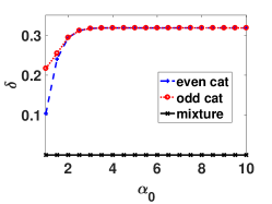
Figure 27: The Wigner negativity $\delta$ as a function of the coherent amplitude $\alpha_{0}$, for both the ideal cat-state and the mixture Eq. (25).

The negativity of the Wigner function can be quantified as (Kenfack and Życzkowski, 2004)

$$\delta =\frac{1}{2}\intop\left[\left|W\left(\alpha,\alpha^{*}\right)\right|-W\left(\alpha,\alpha^{*}\right)\right]d^{2}\alpha\,.$$ (41)

A positive-valued Wigner function gives $\delta=0$ while $\delta$ is nonzero in the presence of any negative values in a Wigner function. The Wigner functions $W_{+}$ and $W_{-}$ for the even cat-state and odd cat-state respectively are given by (Teh et al., 2018)

$$W_{\pm}\left(\alpha,\alpha^{*}\right) = \frac{2}{\pi}\mathcal{N}_{\pm}^{2}\left\{exp\left[-2\left(\alpha^{*}-\alpha_{0}^{*}\right)\left(\alpha-\alpha_{0}\right)\right]\right.$$

$$+exp\left[-2\left(\alpha^{*}+\alpha_{0}^{*}\right)\left(\alpha+\alpha_{0}\right)\right]$$

$$\pm\langle\alpha_{0}|-\alpha_{0}\rangle exp\left[-2\left(\alpha^{*}-\alpha_{0}^{*}\right)\left(\alpha+\alpha_{0}\right)\right]$$

$$\left.\pm\langle-\alpha_{0}|\alpha_{0}\rangle exp\left[-2\left(\alpha^{*}+\alpha_{0}^{*}\right)\left(\alpha-\alpha_{0}\right)\right]\right\}\,.$$

which give negative values. For a mixture $\rho$ of Eq. (25) which has purity given by $\mathcal{P}=P_{+}^{2}+P_{-}^{2}+P_{+}P_{-}\text{e}^{-2\left|\alpha_{0}\right|^{2}}$, the Wigner function is

$$W_{\text{mix}}\left(\alpha,\alpha^{*}\right) =\frac{1}{\pi}\left\{exp\left[-2\left(\alpha^{*}-\alpha_{0}^{*}\right)\left(\alpha-\alpha_{0}\right)\right]\right.$$

$$+exp\left[-2\left(\alpha^{*}+\alpha_{0}^{*}\right)\left(\alpha+\alpha_{0}\right)\right]$$ (43)

and does not admit any negative values. Fig. 27 plots the value of $\delta$, using Eq. (41), for the cat-states $|\psi_{\text{even}}\rangle$ and $|\psi_{\text{odd}}\rangle$ versus $\alpha_{0}$, and for the mixture $\rho$ of Eq. (25) with $P_{+}=P_{-}=1/2$, which has purity given by $\mathcal{P}=\left(2+e^{-4\left|\alpha_{0}\right|^{2}}\right)/4$. Hence, the magnitude of Wigner function negativity $\delta$ quantitatively captures the nonclassicality of the quantum state. This is because the mixture Eq. (25) has a non-negative Wigner function. Hence, if we assume the system is constrained to the manifold of superpositions of the two coherent state (or their mixtures), the negativity is a signature of a cat-state. We note however that more generally, the negativity does not always imply a cat-state, due to the possible presence of microscopic superpositions.

Numerically, the computation of the Wigner negativity in Eq. (41) requires schemes of numerical integration that have errors as a finite grid size is used. In this work, a trapezoidal numerical integration as well as the Gauss-Lobatto numerical integration are used. With the same grid size, the Gauss-Lobatto method is known to be much more accurate than the trapezoidal numerical integration. The Wigner negativities computed using both of these methods agree up to four significant figures, indicating that the grid size chosen is fine enough and the Wigner negativities computed have small grid size errors.

A.3.2 Husimi Q function

The Husimi Q function is defined by $Q\left(\alpha,\alpha^{*}\right)=\langle\alpha|\rho|\alpha\rangle/\pi$. The expression of a Q function for a density operator in the number state basis is given by

$$Q\left(\alpha,\alpha^{*}\right) =\frac{1}{\pi}\langle\alpha|\rho|\alpha\rangle$$

$$=\frac{1}{\pi}\langle\alpha|\left(\sum_{n,m}\rho_{nm}|n\rangle\langle m|\right)|\alpha\rangle$$

$$=\sum_{n,m}\rho_{nm}\frac{\left(\alpha^{*}\right)^{n}\alpha^{m}}{\pi\sqrt{n!m!}}exp\left(-\left|\alpha\right|^{2}\right)\,.$$ (44)

Unlike the Wigner function which admits negative values and is used as an indicator of nonclassicality, the Husimi Q function is always positive. However, it has been shown by Lütkenhaus and Barnett (Lütkenhaus and Barnett, 1995) that a highly nonclassical state will have zeros in the Q function, where the corresponding Wigner function at these zero points have equal positive and negative contributions. Also, in the case where the calculation of the Wigner function is too numerically intensive to be computed, the Q function can serve as a phase-space visualization guide that complements other cat state signatures.

References

- Schrödinger (1935) E. Schrödinger, Naturwissenschaften 23, 823 (1935).
- Fröwis et al. (2018) F. Fröwis, P. Sekatski, W. Dür, N. Gisin, and N. Sangouard, Rev. Mod. Phys. 90, 025004 (2018).
- Chuang et al. (1997) I. L. Chuang, D. W. Leung, and Y. Yamamoto, Phys. Rev. A 56, 1114 (1997).
- Zurek (2001) W. H. Zurek, Nature 412, 712 (2001).
- van Enk and Hirota (2001) S. J. van Enk and O. Hirota, Phys. Rev. A 64, 022313 (2001).
- Toscano et al. (2006) F. Toscano, D. A. R. Dalvit, L. Davidovich, and W. H. Zurek, Phys. Rev. A 73, 023803 (2006).
- Caves and Shaji (2010) C. M. Caves and A. Shaji, Optics Communications 283, 695 (2010).
- Joo et al. (2011) J. Joo, W. J. Munro, and T. P. Spiller, Phys. Rev. Lett. 107, 083601 (2011).
- Mirrahimi et al. (2014) M. Mirrahimi, Z. Leghtas, V. V. Albert, S. Touzard, R. J. Schoelkopf, L. Jiang, and M. H. Devoret, New Journal of Physics 16, 045014 (2014).
- Wang et al. (2016) C. Wang, Y. Y. Gao, P. Reinhold, R. W. Heeres, N. Ofek, K. Chou, C. Axline, M. Reagor, J. Blumoff, K. M. Sliwa, L. Frunzio, S. M. Girvin, L. Jiang, M. Mirrahimi, M. H. Devoret, and R. J. Schoelkopf, Science 352, 1087 (2016).
- Michael et al. (2016) M. H. Michael, M. Silveri, R. T. Brierley, V. V. Albert, J. Salmilehto, L. Jiang, and S. M. Girvin, Phys. Rev. X 6, 031006 (2016).
- Brune et al. (1996) M. Brune, E. Hagley, J. Dreyer, X. Maître, A. Maali, C. Wunderlich, J. M. Raimond, and S. Haroche, Phys. Rev. Lett. 77, 4887 (1996).
- Monroe et al. (1996) C. Monroe, D. M. Meekhof, B. E. King, and D. J. Wineland, Science 272, 1131 (1996).
- Friedman et al. (2000) J. R. Friedman, V. Patel, W. Chen, S. K. Tolpygo, and J. E. Lukens, Nature 406, 43 (2000).
- Greiner et al. (2002) M. Greiner, O. Mandel, T. W. Hänsch, and I. Bloch, Nature 419, 51 (2002).
- Walther et al. (2004) P. Walther, J.-W. Pan, M. Aspelmeyer, R. Ursin, S. Gasparoni, and A. Zeilinger, Nature 429, 158 (2004).
- Mitchell et al. (2004) M. W. Mitchell, J. S. Lundeen, and A. M. Steinberg, Nature 429, 161 (2004).
- Leibfried et al. (2005) D. Leibfried, E. Knill, S. Seidelin, J. Britton, R. B. Blakestad, J. Chiaverini, D. B. Hume, W. M. Itano, J. D. Jost, C. Langer, R. Ozeri, R. Reichle, and D. J. Wineland, Nature 438, 639 (2005).
- Ourjoumtsev et al. (2007) A. Ourjoumtsev, H. Jeong, R. Tualle-Brouri, and P. Grangier, Nature 448, 784 (2007).
- Palacios-Laloy et al. (2010) A. Palacios-Laloy, F. Mallet, F. Nguyen, P. Bertet, D. Vion, D. Esteve, and A. N. Korotkov, Nature Physics 6, 442 (2010).
- Afek et al. (2010) I. Afek, O. Ambar, and Y. Silberberg, Science 328, 879 (2010).
- Monz et al. (2011) T. Monz, P. Schindler, J. T. Barreiro, M. Chwalla, D. Nigg, W. A. Coish, M. Harlander, W. Hänsel, M. Hennrich, and R. Blatt, Phys. Rev. Lett. 106, 130506 (2011).
- Kirchmair et al. (2013) G. Kirchmair, B. Vlastakis, Z. Leghtas, S. E. Nigg, H. Paik, E. Ginossar, M. Mirrahimi, L. Frunzio, S. M. Girvin, and R. J. Schoelkopf, Nature 495, 205 (2013).
- Kovachy et al. (2015) T. Kovachy, P. Asenbaum, C. Overstreet, C. A. Donnelly, S. M. Dickerson, A. Sugarbaker, J. M. Hogan, and M. A. Kasevich, Nature 528, 530 (2015).
- Omran et al. (2019) A. Omran, H. Levine, A. Keesling, G. Semeghini, T. T. Wang, S. Ebadi, H. Bernien, A. S. Zibrov, H. Pichler, S. Choi, J. Cui, M. Rossignolo, P. Rembold, S. Montangero, T. Calarco, M. Endres, M. Greiner, V. Vuletić, and M. D. Lukin, Science 365, 570 (2019).
- Vlastakis et al. (2013) B. Vlastakis, G. Kirchmair, Z. Leghtas, S. E. Nigg, L. Frunzio, S. M. Girvin, M. Mirrahimi, M. H. Devoret, and R. J. Schoelkopf, Science 342, 607 (2013).
- Leghtas et al. (2015) Z. Leghtas, S. Touzard, I. M. Pop, A. Kou, B. Vlastakis, A. Petrenko, K. M. Sliwa, A. Narla, S. Shankar, M. J. Hatridge, M. Reagor, L. Frunzio, R. J. Schoelkopf, M. Mirrahimi, and M. H. Devoret, Science 347, 853 (2015).
- Wang et al. (2019) Z. Wang, M. Pechal, E. A. Wollack, P. Arrangoiz-Arriola, M. Gao, N. R. Lee, and A. H. Safavi-Naeini, Phys. Rev. X 9, 021049 (2019).
- Wallraff et al. (2004) A. Wallraff, D. I. Schuster, A. Blais, L. Frunzio, R. S. Huang, J. Majer, S. Kumar, S. M. Girvin, and R. J. Schoelkopf, Nature 431, 162 (2004).
- Leghtas et al. (2013a) Z. Leghtas, G. Kirchmair, B. Vlastakis, M. H. Devoret, R. J. Schoelkopf, and M. Mirrahimi, Phys. Rev. A 87, 042315 (2013a).
- Leghtas et al. (2013b) Z. Leghtas, G. Kirchmair, B. Vlastakis, R. J. Schoelkopf, M. H. Devoret, and M. Mirrahimi, Phys. Rev. Lett. 111, 120501 (2013b).
- Drummond and Kinsler (1989) P. D. Drummond and P. Kinsler, Phys. Rev. A 40, 4813 (1989).
- Kinsler and Drummond (1991) P. Kinsler and P. D. Drummond, Phys. Rev. A 43, 6194 (1991).
- Marandi et al. (2014) A. Marandi, Z. Wang, K. Takata, R. L. Byer, and Y. Yamamoto, Nature Photonics 8, 937 (2014).
- McMahon et al. (2016) P. L. McMahon, A. Marandi, Y. Haribara, R. Hamerly, C. Langrock, S. Tamate, T. Inagaki, H. Takesue, S. Utsunomiya, K. Aihara, R. L. Byer, M. M. Fejer, H. Mabuchi, and Y. Yamamoto, Science 354, 614 (2016).
- Inagaki et al. (2016) T. Inagaki, Y. Haribara, K. Igarashi, T. Sonobe, S. Tamate, T. Honjo, A. Marandi, P. L. McMahon, T. Umeki, K. Enbutsu, O. Tadanaga, H. Takenouchi, K. Aihara, K.-i. Kawarabayashi, K. Inoue, S. Utsunomiya, and H. Takesue, Science 354, 603 (2016).
- Nigg et al. (2012) S. E. Nigg, H. Paik, B. Vlastakis, G. Kirchmair, S. Shankar, L. Frunzio, M. H. Devoret, R. J. Schoelkopf, and S. M. Girvin, Phys. Rev. Lett. 108, 240502 (2012).
- Goto et al. (2019) H. Goto, Z. Lin, T. Yamamoto, and Y. Nakamura, Phys. Rev. A 99, 023838 (2019).
- Pfaff et al. (2017) W. Pfaff, C. J. Axline, L. D. Burkhart, U. Vool, P. Reinhold, L. Frunzio, L. Jiang, M. H. Devoret, and R. J. Schoelkopf, Nature Physics 13, 882 (2017).
- Goto (2016a) H. Goto, Scientific Reports 6, 21686 (2016a).
- Goto (2016b) H. Goto, Phys. Rev. A 93, 050301 (2016b).
- Puri et al. (2017) S. Puri, C. K. Andersen, A. L. Grimsmo, and A. Blais, Nature Communications 8, 15785 (2017).
- Brosnan and Byer (1979) S. Brosnan and R. Byer, IEEE Journal of Quantum Electronics 15, 415 (1979).
- Heidmann et al. (1987) A. Heidmann, R. J. Horowicz, S. Reynaud, E. Giacobino, C. Fabre, and G. Camy, Phys. Rev. Lett. 59, 2555 (1987).
- Villar et al. (2005) A. S. Villar, L. S. Cruz, K. N. Cassemiro, M. Martinelli, and P. Nussenzveig, Phys. Rev. Lett. 95, 243603 (2005).
- Laurat et al. (2005) J. Laurat, L. Longchambon, C. Fabre, and T. Coudreau, Opt. Lett. 30, 1177 (2005).
- Keller et al. (2008) G. Keller, V. D’Auria, N. Treps, T. Coudreau, J. Laurat, and C. Fabre, Opt. Express 16, 9351 (2008).
- Drummond et al. (1981) P. Drummond, K. McNeil, and D. Walls, Optica Acta: International Journal of Optics 28, 211 (1981).
- Wolinsky and Carmichael (1988) M. Wolinsky and H. J. Carmichael, Phys. Rev. Lett. 60, 1836 (1988).
- Reid and Yurke (1992) M. D. Reid and B. Yurke, Phys. Rev. A 46, 4131 (1992).
- Gilles et al. (1994) L. Gilles, B. M. Garraway, and P. L. Knight, Phys. Rev. A 49, 2785 (1994).
- Hach III and Gerry (1994) E. E. Hach III and C. C. Gerry, Phys. Rev. A 49, 490 (1994).
- Krippner et al. (1994) L. Krippner, W. J. Munro, and M. D. Reid, Phys. Rev. A 50, 4330 (1994).
- Sun et al. (2019a) F.-X. Sun, Q. He, Q. Gong, R. Y. Teh, M. D. Reid, and P. D. Drummond, New Journal of Physics, 21, 093035 (2019a).
- Sun et al. (2019b) F.-X. Sun, Q. He, Q. Gong, R. Y. Teh, M. D. Reid, and P. D. Drummond, Phys. Rev. A 100, 033827 (2019b).
- Yurke and Stoler (1986) B. Yurke and D. Stoler, Phys. Rev. Lett. 57, 13 (1986).
- Yurke and Stoler (1988) B. Yurke and D. Stoler, Physica B+C 151, 298 (1988).
- Wigner (1932) E. Wigner, Phys. Rev. 40, 749 (1932).
- Cahill and Glauber (1969) K. E. Cahill and R. J. Glauber, Phys. Rev. 177, 1882 (1969).
- Hillery et al. (1984) M. Hillery, R. O’Connell, M. Scully, and E. Wigner, Physics Reports 106, 121 (1984).
- Kenfack and Życzkowski (2004) A. Kenfack and K. Życzkowski, Journal of Optics B: Quantum and Semiclassical Optics 6, 396 (2004).
- Lütkenhaus and Barnett (1995) N. Lütkenhaus and S. M. Barnett, Phys. Rev. A 51, 3340 (1995).
- Yurke (1984) B. Yurke, Phys. Rev. A 29, 408 (1984).
- Yurke and Denker (1984) B. Yurke and J. S. Denker, Phys. Rev. A 29, 1419 (1984).
- Collett and Gardiner (1984) M. J. Collett and C. W. Gardiner, Phys. Rev. A 30, 1386 (1984).
- Gardiner and Collett (1985) C. W. Gardiner and M. J. Collett, Phys. Rev. A 31, 3761 (1985).
- Drummond et al. (1980) P. D. Drummond, K. J. McNeil, and D. F. Walls, Optica Acta: International Journal of Optics, Optica Acta: International Journal of Optics 27, 321 (1980).
- Munro and Reid (1995) W. J. Munro and M. D. Reid, Phys. Rev. A 52, 2388 (1995).
- Bužek et al. (1992) V. Bužek, A. Vidiella-Barranco, and P. L. Knight, Phys. Rev. A 45, 6570 (1992).
- Gilles and Knight (1993) L. Gilles and P. L. Knight, Phys. Rev. A 48, 1582 (1993).
- Carmichael and Wolinsky (1986) H. J. Carmichael and M. Wolinsky, in Quantum Optics IV, edited by J. D. Harvey and D. F. Walls (Springer Berlin Heidelberg, Berlin, Heidelberg, 1986) pp. 208–220.
- Drummond and Gardiner (1980) P. D. Drummond and C. W. Gardiner, Journal of Physics A: Mathematical and General 13, 2353 (1980).
- Kryuchkyan and Kheruntsyan (1996) G. Kryuchkyan and K. Kheruntsyan, Optics Communications 127, 230 (1996).
- Carmichael (2009) H. J. Carmichael, Statistical methods in quantum optics 2: Non-classical fields (Springer Science & Business Media, 2009).
- Lugiato et al. (1988) L. A. Lugiato, C. Oldano, C. Fabre, E. Giacobino, and R. J. Horowicz, Il Nuovo Cimento D 10, 959 (1988).
- Fabre et al. (1990) C. Fabre, E. Giacobino, A. Heidmann, L. Lugiato, S. Reynaud, M. Vadacchino, and W. Kaige, Quantum Optics: Journal of the European Optical Society Part B 2, 159 (1990).
- Drummond and Walls (1980) P. D. Drummond and D. F. Walls, Journal of Physics A: Mathematical and General 13, 725 (1980).
- Deuar and Drummond (2002) P. Deuar and P. D. Drummond, Phys. Rev. A 66, 033812 (2002).
- Bennett et al. (1996) C. H. Bennett, H. J. Bernstein, S. Popescu, and B. Schumacher, Phys. Rev. A 53, 2046 (1996).
- Terhal and Horodecki (2000) B. M. Terhal and P. Horodecki, Phys. Rev. A 61, 040301(R) (2000).
- Brennen (2003) G. K. Brennen, Quantum Info. Comput. 3, 619 (2003).
- Cavalcanti and Reid (2006) E. G. Cavalcanti and M. D. Reid, Phys. Rev. Lett. 97, 170405 (2006).
- Korsbakken et al. (2007) J. I. Korsbakken, K. B. Whaley, J. Dubois, and J. I. Cirac, Phys. Rev. A 75, 042106 (2007).
- Cavalcanti and Reid (2008) E. G. Cavalcanti and M. D. Reid, Phys. Rev. A 77, 062108 (2008).
- Fröwis and Dür (2012) F. Fröwis and W. Dür, New Journal of Physics 14, 093039 (2012).
- Baumgratz et al. (2014) T. Baumgratz, M. Cramer, and M. B. Plenio, Phys. Rev. Lett. 113, 140401 (2014).
- Sekatski et al. (2014) P. Sekatski, N. Sangouard, and N. Gisin, Phys. Rev. A 89, 012116 (2014).
- Fröwis et al. (2015) F. Fröwis, N. Sangouard, and N. Gisin, Optics Communications 337, 2 (2015), macroscopic quantumness: theory and applications in optical sciences.
- Oudot et al. (2015) E. Oudot, P. Sekatski, F. Fröwis, N. Gisin, and N. Sangouard, J. Opt. Soc. Am. B 32, 2190 (2015).
- Fröwis et al. (2016) F. Fröwis, P. Sekatski, and W. Dür, Phys. Rev. Lett. 116, 090801 (2016).
- Yadin and Vedral (2016) B. Yadin and V. Vedral, Phys. Rev. A 93, 022122 (2016).
- Teh et al. (2018) R. Y. Teh, S. Kiesewetter, P. D. Drummond, and M. D. Reid, Phys. Rev. A 98, 063814 (2018).
- Reid (2019) M. Reid, Physical Review A 100, 052118 (2019).
- Polkinghorne (2019) R. Polkinghorne, Fock States (https://www.github.com/thisrod/fockstates), GitHub (2019).
- Clenshaw (1955) C. W. Clenshaw, Mathematics of Computation 9, 118 (1955).
- Press et al. (2007) W. Press, S. Teukolsky, W. Vetterling, and B. Flannery, Numerical Recipes 3rd Edition: The Art of Scientific Computing (Cambridge University Press, 2007).
- Smith (1965) F. J. Smith, Mathematics of Computation 19, 33 (1965).
- Forsythe (1957) G. Forsythe, Journal of the Society for Industrial and Applied Mathematics 5, 74 (1957).
- Pathak and Banerji (2014) A. Pathak and J. Banerji, Physics Letters A 378, 117 (2014).
- Lutterbach and Davidovich (1997) L. G. Lutterbach and L. Davidovich, Phys. Rev. Lett. 78, 2547 (1997).
- Bertet et al. (2002) P. Bertet, A. Auffeves, P. Maioli, S. Osnaghi, T. Meunier, M. Brune, J. M. Raimond, and S. Haroche, Phys. Rev. Lett. 89, 200402 (2002).
- Sun et al. (2014) L. Sun, A. Petrenko, Z. Leghtas, B. Vlastakis, G. Kirchmair, K. M. Sliwa, A. Narla, M. Hatridge, S. Shankar, J. Blumoff, L. Frunzio, M. Mirrahimi, M. H. Devoret, and R. J. Schoelkopf, Nature 511, 444 (2014).
- Liu et al. (2017) K. Liu, Y. Xu, W. Wang, S.-B. Zheng, T. Roy, S. Kundu, M. Chand, A. Ranadive, R. Vijay, Y. Song, L. Duan, and L. Sun, Science Advances 3 (2017), 10.1126/sciadv.1603159.
- Wang et al. (2017) W. Wang, L. Hu, Y. Xu, K. Liu, Y. Ma, S.-B. Zheng, R. Vijay, Y. P. Song, L.-M. Duan, and L. Sun, Phys. Rev. Lett. 118, 223604 (2017).