RKKY interactions of CeB₆ based on effective Wannier model

Abstract

We examine the RKKY interactions of CeB₆ between multipole moments based on the effective Wannier model obtained from the bandstructure calculation including 14 Ce-$f$ orbitals and 60 conduction orbitals of Ce-$d,s$ and B-$p,s$. By using the $f$-$c$ mixing matrix elements of the Wannier model together with the conduction band dispersion, the multipole couplings with the RKKY oscillation are obtained for the active moments in $\Gamma_{8}$ subspace. Both of the $\Gamma_{5g}$ quadrupole $O_{xy}$ and the $\Gamma_{2u}$ octupole $T_{xyz}$ couplings are largely enhanced with $\bm{q}=(\pi,\pi,\pi)$ which naturally explains the antiferro-quadrupolar phase of the phase II, and are also enhanced with $\bm{q}=(0,0,0)$ corresponding to the elastic softening of $C_{44}$. Also the couplings of the $\Gamma_{5u}$ octupole $T_{z}^{\beta}$ is quite large for $\bm{q}=(0,0,\pi)$ which is related to the antiferro-octupolar ordering of a possible candidate for the phase IV of Ce_xLa_1-xB₆.

1 Introduction

Electronic state of CeB₆ has been one of the central issues in the heavy Fermion systems, since it exhibits a rich phase diagram of the multipole orderings[1, 2] due to the $\Gamma_{8}$ quartet ground state with the degrees of freedom of multipole moments as shown in Table 1. Several multipole orderings have been observed in temperature and magnetic field $(T,H)$ phase diagram such as the antifero-quadrupolar (AFQ) ordering of $\Gamma_{5g}$ quadrupole moments $(O_{yz},O_{zx},O_{xy})$ with a critical transition temperature $T_{Q}=3.2$ K (phase II) and the antifero-magnetic ordering of $\Gamma_{4u}$ magnetic multipoles $(\sigma^{x},\sigma^{y},\sigma^{z})$ with $T_{N}=2.3$ K (phase III). The antifero-octupolar (AFO) ordering of $\Gamma_{5u}$ octupoles $(T^{\beta}_{x},T^{\beta}_{y},T^{\beta}_{z})$ is also discussed as a possible candidate of the phase IV in the La-substitution system of Ce_xLa_1-xB₆.

The 4$f$ electrons of CeB₆ are almost localized from several experiments. The Fermi-surface (FS) has been observed in the de Haas-van Alphen (dHvA) experiments[3], the angle resolved photoemission spectroscopy (ARPES)[4, 5] and the high-resolution photoemission tomography[6], where an ellipsoidal FS centered at X point in the Brillouin zone (BZ) has been confirmed and is almost the same as that of LaB₆ with the 4$f^{0}$ state. In such a localized $f$ electron system, Ruderman-Kittel-Kasuya-Yosida (RKKY) interaction[7, 8, 9] plays an important role for the multipole ordering and must determine the ordering moments and wavevectors. The phonomenological RKKY models of CeB₆[10, 11] succeeded in reproducing the basic phase diagram in $T$-$H$ plane and giving a great advance in the multipole physics in $\Gamma_{8}$ ground state system.

However in these studies, only the nearest neighbor RKKY Hamiltonian with a symmetric coupling and/or asymmetric correction terms was used for explaining the experimental phase diagram. As shown in the original studies[7, 8, 9], the RKKY interaction has a decaying and oscillating function of $2k_{\rm F}R$ with the Fermi wavenumber $k_{\rm F}$ of conduction $(c)$ band and distance between multipole moments $R$, and thus these effects should be taken into account through the microscopic description of the $f$-$c$ mixing and $c$ band states. The explicit derivation of the RKKY multipole couplings based on the realistic bandstructure calculation still has been an important challenge for the microscopic understanding of the multipole order.

In this study, we derive the RKKY interaction of CeB₆ based on the 74-orbital effective Wannier model derived from the bandstructure calculation directly[12]. By using the realistic $c$ band dispersion together with the $f$-$c$ mixing matrix elements from the Wannier model of CeB₆, we calculate the RKKY couplings between the active multipole moments in $\Gamma_{8}$ subspace mediated by the realistic $c$ band states explicitly. The obtained RKKY multipole interactions show that the 1st leading multipole mode is the $\bm{q}=(\pi,\pi,\pi)$-AFQ ordering with $\Gamma_{5g}$ quadrupole $O_{xy}$ together with $\Gamma_{2u}$ octupole $T_{xyz}$ and the 2nd leading mode is the $\bm{q}=(0,0,\pi)$-AFO ordering with $\Gamma_{5u}$ octupole $T_{z}^{\beta}$.

IRR	notation	pseudospin rep.	multipole
$\Gamma_{2u}$	$\xi$	$\tau^{y}$	$\frac{2}{9\sqrt{5}}T_{xyz}$
$\Gamma_{3g}$	$\bm{\tau}^{\prime}{}=(\tau^{z},\tau^{x})$	$(\tau^{z},\tau^{x})$	$\frac{1}{4}(O_{u},O_{v})$
$\Gamma_{5g}$	$\bm{\mu}=(\mu^{x},\mu^{y},\mu^{z})$	$(\tau^{y}\sigma^{x},\tau^{y}\sigma^{y},\tau^{y}\sigma^{z})$	$(O_{yz},O_{zx},O_{xy})$
$\Gamma_{4u}^{(1)}$	$\bm{\sigma}=(\sigma^{x},\sigma^{y},\sigma^{z})$	$(\sigma^{x},\sigma^{y},\sigma^{z})$	$\frac{14}{15}\bm{J}-\frac{4}{45}\bm{T}^{\alpha}$
$\Gamma_{4u}^{(2)}$	$\bm{\eta}=(\eta^{x},\eta^{y},\eta^{z})$	$(\eta^{+}\sigma^{x},\eta^{-}\sigma^{y},\tau^{z}\sigma^{z})$	$-\frac{2}{15}\bm{J}+\frac{7}{45}\bm{T}^{\alpha}$
$\Gamma_{5u}$	$\bm{\zeta}=(\zeta^{x},\zeta^{y},\zeta^{z})$	$(\zeta^{+}\sigma^{x},\zeta^{-}\sigma^{y},\tau^{x}\sigma^{z})$	$\frac{1}{3\sqrt{5}}\bm{T}^{\beta}$

Table 1: The irreducible representations (IRRs), notations and pseudospin representations for the active multipole moments in $\Gamma_{8}$ subspace where $\bm{J}~{}(\bm{T}^{\alpha,\beta})$ is the dipole (octupole), $\bm{J}=(J_{x},J_{y},J_{z})$, $\bm{T}^{\alpha(\beta)}=(T_{x}^{\alpha(\beta)},T_{y}^{\alpha(\beta)},T_{z}^{\alpha(\beta)})$, $\eta^{\pm}=-\frac{1}{2}(\tau^{z}\mp\sqrt{3}\tau^{x})$, $\zeta^{\pm}=-\frac{1}{2}(\tau^{x}\pm\sqrt{3}\tau^{z})$, and $g~{}(u)$ means even (odd) time-reversal symmetry. Here all the multipole operators are normalized.

2 Model & Formulation

First we perform the bandstructure calculation of CeB₆ and LaB₆ by using the WIEN2k code[13], which is based on the density-functional theory (DFT) and includes the effect of the spin-orbit coupling (SOC) within the second variation approximation. The explicit bandstructures and FSs are shown in Fig.1 (a)-(d) of Ref. [12], where three FSs are obtained in CeB₆, while an ellipsoidal FS centered at X point is obtained in LaB₆, which well accounts for the experimental results[3, 4, 5, 6].

Next we construct the 74-orbital effective Wannier model based on the maximally localized Wannier functions (MLWFs) method[14, 15] from the DFT bandstructure of CeB₆, where 14 $f$-states from Ce-$f$ (7 orbital $\times$ 2 spin) and 60 $c$-states from Ce-$d$ (5 orbital $\times$ 2 spin), Ce-$s$ (1 orbital $\times$ 2 spin), B-$p$ (6 site $\times$ 3 orbital $\times$ 2 spin) and B-$s$ (6 site $\times$ 1 orbital $\times$ 2 spin) are fully included and the obtained bandstructure well reproduces the DFT band as shown in Fig.1 (e) and (f) of Ref. [12]. The obtained tight-binding (TB) Hamiltonian is given by the following form as,

$$H_{\rm TB} =\sum_{\bm{k}}\sum_{mm^{\prime}{}}h_{mm^{\prime}{}}^{ff}(\bm{k})f_{\bm{k}m}^{\dagger}f_{\bm{k}m^{\prime}{}}+\sum_{\bm{k}}\sum_{\ell\ell^{\prime}{}}h_{\ell\ell^{\prime}{}}^{cc}(\bm{k})c_{\bm{k}\ell}^{\dagger}c_{\bm{k}\ell^{\prime}{}}+\sum_{\bm{k}}\sum_{m\ell}\left(V_{\bm{k}m\ell}f_{\bm{k}m}^{\dagger}c_{\bm{k}\ell}+h.c.\right)$$ (1)

where $f_{\bm{k}m}^{\dagger}~{}(c_{\bm{k}\ell}^{\dagger})$ is a creation operator for a $f~{}(c)$ electron with wavevector $\bm{k}$ and 14 (60) spin-orbital states $m~{}(\ell)$. Here 14 $f$ states of $m$ are represented by the CEF eigenstates as $\Gamma_{8}$ quartet and $\Gamma_{7}$ doublet with the total angular momentum $J=5/2$, and $\Gamma_{6}$, $\Gamma_{7}$ doublets and $\Gamma_{8}$ quartet with $J=7/2$. The $f$-$f$ [$c$-$c$] matrix element of $h_{mm^{\prime}{}}^{ff}(\bm{k})~{}[h_{\ell\ell^{\prime}{}}^{cc}(\bm{k})]$ includes the $f~{}(c)$ energy levels, SOC couplings, CEF splittings and $f$-$f$ ($c$-$c$) hopping integrals, and $V_{\bm{k}m\ell}$ is the $f$-$c$ mixing element.

Here we consider the RKKY interaction between the multipole moments of $\Gamma_{8}$ quartet. For this purpose, we start from the localized $f$ limit where a $4f^{1}$ state is realized in $\Gamma_{8}$ at each Ce site and the $f$-$f$ hopping and $f$-$c$ mixing become zero. Hence the remained $c$ electron Hamiltonian $H_{\rm TB}^{c}$ is diagonalized as follows,

$$H_{\rm TB}^{c}=\sum_{\bm{k}}\sum_{\ell\ell^{\prime}{}}h_{\ell\ell^{\prime}{}}^{cc}(\bm{k})c_{\bm{k}\ell}^{\dagger}c_{\bm{k}\ell^{\prime}{}}=\sum_{\bm{k}s}\varepsilon_{\bm{k}s}^{c}a_{\bm{k}s}^{\dagger}a_{\bm{k}s},$$ (2)

where $a_{\bm{k}s}^{\dagger}$ is a creation operator for a electron with $\bm{k}$ and band-index $s$ with the $c$ band dispersion $\varepsilon_{\bm{k}s}^{c}$ and the eigenvector $u_{\bm{k}s\ell}^{c}$ where $a_{\bm{k}s}=\sum_{\ell}u_{\bm{k}s\ell}^{c}c_{\bm{k}\ell}$. Figure 1 shows the $c$ bandstructure [Fig. 1(a)] and their FSs of the 21st band [Fig. 1(b) & (c)] and the obtained $c$ state well describes the experimental FSs[3, 4, 5, 6] and is also almost same as the DFT-bandstructure of LaB₆ without $f$ electron.

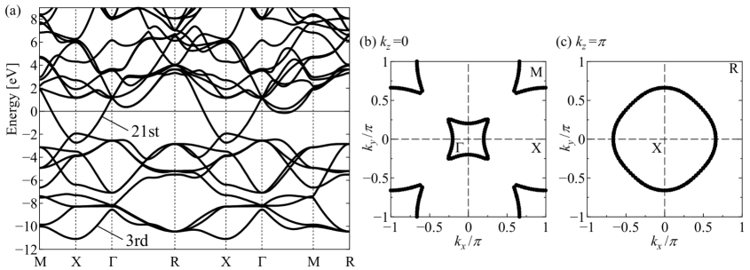
Figure 1: (a) Bandstructure and (b),(c) FSs (21st band) of the conduction states in the Wannier model for CeB₆ in the simple cubic BZ, where the high-symmetry points are $\Gamma$[$(0,0,0)$], X[$(\pi,0,0)$], M[$(\pi.\pi,0)$] and R[$(\pi.\pi,\pi)$]. All bands have two-folded degeneracy due to the time-reversal symmetry and 1st and 2nd bands are located in $-15$ eV (not shown).

By using the second-order perturbation w. r. t. the $f$-$c$ mixing $V_{\bm{k}m\ell}$ in the third term of $H_{\rm TB}$, we obtain the multi-orbital Kondo lattice Hamiltonian which is given by,

$$H_{\rm MKL} =\sum_{im}\left(\varepsilon_{\Gamma_{8}}^{f}+\Delta\varepsilon_{\Gamma_{8}}^{f}\right)f_{im}^{\dagger}f_{im}+\sum_{\bm{k}s}\varepsilon_{\bm{k}s}^{c}a_{\bm{k}s}^{\dagger}a_{\bm{k}s}+\sum_{i}\sum_{mm^{\prime}{}}\sum_{\bm{k}\bm{k^{\prime}{}}}\sum_{\ell\ell^{\prime}{}}J_{imm^{\prime}{}}^{\bm{k}\ell,\bm{k}^{\prime}{}\ell^{\prime}{}}f_{im}^{\dagger}f_{im^{\prime}{}}c_{\bm{k}\ell}^{\dagger}c_{\bm{k}^{\prime}{}\ell^{\prime}{}},$$ (3)

where $f_{im}^{\dagger}$ is a creation operator for a $f$ electron with a Ce-atom $i$ and 4-states in $\Gamma_{8}$ quartet $\Ket{m}=\Ket{1}\sim\Ket{4}$ which are given with the $J_{z}$-base of $J=5/2$ $\Ket{M}$ explicitly as,

$$\Ket{1}=-\sqrt{\frac{1}{6}}\Ket{+\frac{3}{2}}-\sqrt{\frac{5}{6}}\Ket{-\frac{5}{2}}$$ (4)

$$\Ket{2}=+\Ket{+\frac{1}{2}}$$ (5)

$$\Ket{3}=-\Ket{-\frac{1}{2}}$$ (6)

$$\Ket{4}=+\sqrt{\frac{1}{6}}\Ket{-\frac{3}{2}}+\sqrt{\frac{5}{6}}\Ket{+\frac{5}{2}},$$ (7)

where $\varepsilon_{\Gamma_{8}}^{f}$ is the bare $f$ energy-level and $\Delta\varepsilon_{\Gamma_{8}}^{f}$ is a energy shift due to the DFT potential which is of the order of a few eV. The Kondo coupling $J_{imm^{\prime}{}}^{\bm{k}\ell,\bm{k}^{\prime}{}\ell^{\prime}{}}$ can be written by the following simple form,

$$J_{imm^{\prime}{}}^{\bm{k}\ell,\bm{k}^{\prime}{}\ell^{\prime}{}}=\frac{2}{N}\frac{V_{\bm{k}m\ell}V_{\bm{k}^{\prime}{}m^{\prime}{}\ell^{\prime}{}}^{*}}{\mu-\varepsilon_{\Gamma_{8}}^{f}}e^{-i(\bm{k}-\bm{k}^{\prime}{})\cdot\bm{R}_{i}},$$ (8)

where only $f^{0}$-intermediate process is considered and the scattered $c$ orbital energies are fixed to $\mu$.

The RKKY Hamiltonian can be obtained from the second-order perturbation w. r. t. the third term of $H_{\rm MKL}$ together with the thermal average for the $c$ states. The final form is given by,

$$H_{\rm RKKY}\!=\!-\!\sum_{\Braket{ij}}\!\sum_{m_{1}m_{2}}\!\sum_{m_{3}m_{4}}\!K_{m_{1}m_{2}m_{3}m_{4}}(\bm{R}_{ij})f_{im_{1}}^{\dagger}f_{im_{2}}f_{jm_{4}}^{\dagger}f_{jm_{3}},$$ (9)

$$K_{m_{1}m_{2}m_{3}m_{4}}(\bm{R}_{ij})=\frac{1}{N}\sum_{\bm{q}}K_{m_{1}m_{2}m_{3}m_{4}}(\bm{q})~{}e^{i\bm{q}\cdot(\bm{R}_{i}-\bm{R}_{j})},$$ (10)

where $K_{m_{1}m_{2}m_{3}m_{4}}(\bm{R}_{ij})$ is the RKKY coupling between $\{m_{1},m_{2}\}$ at Ce-atom $\bm{R}_{i}$ and $\{m_{3},m_{4}\}$ at $\bm{R}_{j}$ and $\Braket{ij}$ represents a summation for Ce-Ce vectors $\bm{R}_{ij}=\bm{R}_{i}-\bm{R}_{j}$ and $K_{m_{1}m_{2}m_{3}m_{4}}(\bm{q})$ is given by,

$$K_{m_{1}m_{2}m_{3}m_{4}}(\bm{q})=\frac{1}{N}\sum_{\bm{k}ss^{\prime}{}}\frac{v_{\bm{k}s}^{m_{3}m_{1}}v_{\bm{k}+\bm{q}s^{\prime}{}}^{m_{2}m_{4}}}{(\mu-\varepsilon_{\Gamma_{8}}^{f})^{2}}\frac{f(\varepsilon_{\bm{k}+\bm{q}s^{\prime}{}}^{c})-f(\varepsilon_{\bm{k}s}^{c})}{\varepsilon_{\bm{k}s}^{c}-\varepsilon_{\bm{k}+\bm{q}s^{\prime}{}}^{c}},$$ (11)

where $f(x)$ is the Fermi distribution function $f(x)=1/(e^{(x-\mu)/T}+1)$ and $\mu$ is a chemical potential. Here $v_{\bm{k}s}^{mm^{\prime}{}}$ is a $f$-$c$ mixing matrix between $m$ and $m^{\prime}{}$ via the $c$ band state with $\bm{k},s$ given by,

$$v_{\bm{k}s}^{mm^{\prime}{}}=\sum_{\ell\ell^{\prime}{}}V_{\bm{k}m\ell}^{*}V_{\bm{k}m^{\prime}{}\ell^{\prime}{}}u_{\bm{k}s\ell}^{c*}u_{\bm{k}s\ell^{\prime}{}}^{c},$$ (12)

which has all information about the $f$ state scattering between $\{m,m^{\prime}{}\}$ through the $c$ state with $\bm{k},s$.

The multipole interaction in $\bm{q}$-space is explicitly given by the follwing form,

$$\overline{K}_{O_{\Gamma}}(\bm{q})=\sum_{m_{1}m_{2}}\sum_{m_{3}m_{4}}O_{m_{1}m_{2}}^{\Gamma}O_{m_{4}m_{3}}^{\Gamma}\left(K_{m_{1}m_{2}m_{3}m_{4}}(\bm{q})-K_{m_{1}m_{2}m_{3}m_{4}}^{\rm loc}\right)$$ (13)

where $O_{mm^{\prime}{}}^{\Gamma}$ is the matrix element of the multipole operator and $K_{m_{1}m_{2}m_{3}m_{4}}^{\rm loc}=(1/N)\sum_{\bm{q}}K_{m_{1}m_{2}m_{3}m_{4}}(\bm{q})$. The mean-field multipole susceptibility $\chi_{O_{\Gamma}}(\bm{q})$ is written by,

$$\chi_{O_{\Gamma}}(\bm{q})=\frac{\chi_{O_{\Gamma}}^{0}(\bm{q})}{1-\chi_{O_{\Gamma}}^{0}(\bm{q})\overline{K}_{O_{\Gamma}}(\bm{q})},$$ (14)

which is enhanced towards the multipole ordering instability for the ordering moment $O_{\Gamma}$ and wavevector $\bm{q}=\bm{Q}$, and diverges at a critical point of the multipole ordering transition temperature $T=T_{O_{\Gamma}}^{\bm{Q}}$ where $\chi_{O_{\Gamma}}^{0}(\bm{q})\overline{K}_{O_{\Gamma}}(\bm{q})$ reaches unity. In the localized $f$ limit, the $\Gamma_{8}$ ground state is degenerate and the single-site susceptibility for all multipole moments exhibits the Curie law, $\chi_{O_{\Gamma}}^{0}(\bm{q})=1/T$, and then the transition temperature for a certain multipole ordering is determined by the condition $T_{O_{\Gamma}}^{\bm{Q}}=\overline{K}_{O_{\Gamma}}^{\rm max}(\bm{Q})$. Therefore the sign and maximum value of $\overline{K}_{O_{\Gamma}}(\bm{q})$ plays an central role for the multipole ordering. Hereafter we set $\mu-\varepsilon_{\Gamma_{8}}^{f}=2$ eV, and $\mu$ is determined so as to keep $n_{tot}=n^{c}=21$ and $T$ is set to $T=0.005$ eV throughout the calculation.

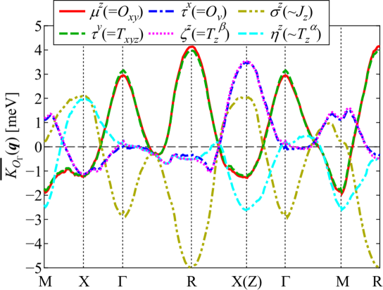
Figure 2: (Color online) The $\bm{q}$-dependence of the RKKY multipole coupling $\overline{K}_{O_{\Gamma}}(\bm{q})$ for the multipole moments of the typical irreducible representations. The individual terms for $\Gamma_{2u}$ octupole $T_{xyz}$, $\Gamma_{3g}$ quadrupoles $O_{u},O_{v}$, $\Gamma_{4u}$ multipoles $(\sigma^{x},\sigma^{y},\sigma^{z})$ and $(\eta^{x},\eta^{y},\eta^{z})$ and, $\Gamma_{5g}$ quadrupoles $(O_{yz},O_{zx},O_{xy})$ and $\Gamma_{5u}$ octupoles $(\zeta^{x},\zeta^{y},\zeta^{z})$.

3 Results

The RKKY couplings $\overline{K}_{O_{\Gamma}}(\bm{q})$ for several multipole moments as a function of the wavevector $\bm{q}$ along the high symmetry line in the BZ are plotted as shown in Fig. 2, where the positive (negative) coupling for a certain multipole with ($O_{\Gamma}$, $\bm{q}$) enhances (suppresses) the corresponding multipole fluctuation and its positive maximum value gives a leading multipole ordering mode. All leading modes are summarized in Table II of Ref. [12].

The couplings of the $\Gamma_{5g}$ quadrupole $O_{xy}$ and $\Gamma_{2u}$ ocutupole $T_{xyz}$ for $\bm{q}=(\pi,\pi,\pi)$ become largest among all moments and $\bm{q}$, which corresponds to the AFQ ordering of CeB₆ as phase II. From the analysis of the real space couplings of $O_{xy}$ and $T_{xyz}$, we have found that the main origin of this mode comes from the fact that the couplings with the 1st and 2nd neighbor Ce-Ce vectors exhibit an anti-ferro (AF) and ferro (F) interaction respectively, which indicates the realization of the RKKY oscillation as shown in Fig. 7 in Ref. [12] but the absolute value of the 2nd neighbor coupling is almost same or slightly larger than that of the 1st neighbor coupling. The 2nd neighbor F couplings of $O_{xy}$ and $T_{xyz}$ also increase the uniform mode with a substantial peak for $\bm{q}=(0,0,0)$ as shown in Fig. 2 corresponding to the elastic softening of $C_{44}$[16].

The difference of the couplings between $O_{xy}$ and $T_{xyz}$ has often been discussed in the early studies[17, 18], where the two couplings must have the same value within the 1st neighbor coupling due to the point group symmetry. In the present calculation, the same coupling value of the 1st neighbor $O_{xy}$ and $T_{xyz}$ has been obtained, while in the 2nd neighbor couplings, a slightly but finite difference between $O_{xy}$ and $T_{xyz}$ has been observed for the Ce-Ce vectors $\bm{R}=a(011),a(101)$ where $a$ is the lattice constant, which enhances the peak of $O_{xy}$ over that of $T_{xyz}$ at $\bm{q}=(\pi,\pi,\pi)$. The anisotropy of the present interaction Hamiltonian including the origin of the above correction together with the so-called ‘bond density’[17] will be presented in the subsequent paper[19].

The next largest coupling is the $\Gamma_{5u}$ octupole $\zeta^{z}$ at $\bm{q}=(0,0,\pi)$ [X(Z) point] which is degenerate for $\zeta^{x}~{}[\zeta^{y}]$ octupole at $\bm{q}=(\pi,0,0)~{}[(0,\pi,0)]$. In addition to this, the $\Gamma_{3g}$ quadrupole $O_{v}=O_{x^{2}-y^{2}}$ coupling is quite large for $\bm{q}=(0,0,\pi)$ and becomes similar value of the octupole coupling $\zeta^{z}$, which is also degenerate for the rotated moments to the each principle-axis $O_{y^{2}-z^{2}}$ and $O_{z^{2}-x^{2}}$ for $\bm{q}=(\pi,0,0)$ and $\bm{q}=(0,\pi,0)$ respectively. In real space, the coupling of $\zeta^{z}$ and $O_{v}$ are highly anisotropic with the AF couplings for the Ce-Ce vector $\bm{R}=a(001)$ and the F couplings for $\bm{R}=a(100),a(010)$, which induces the enhancement of the $\bm{q}=(0,0,\pi)$ mode. In these situation, the triple-$\bm{Q}$ mode of $(\zeta^{x},\zeta^{y},\zeta^{z})$ and $(O_{y^{2}-z^{2}},O_{z^{2}-x^{2}},O_{x^{2}-y^{2}})$ with $\bm{Q}=(\pi,0,0),(0,\pi,0),(0,0,\pi)$ may become possible for the phase IV in Ce_xLa_1-xB₆ with $x<0.8$, which is different from the $\bm{q}=(\pi,\pi,\pi)$ AFO ordering of $(\zeta^{x}+\zeta^{y}+\zeta^{z})/\sqrt{3}$ [20]. The present development of the $\zeta^{z}$ and $O_{v}$ X-point mode appears to be related to the recent inelastic neutron scattering experiments in Ce_xLa_1-xB₆[21], where the intensity $\bm{q}=(\pi,0,0)$ is enhanced and becomes dominant mode for $x<0.8$.

As for the phase III of the AFM order, the $\Gamma_{4u}$ magnetic multipole couplings of $\sigma^{z}$ and $\eta^{z}$ shall be dominant when the system enters into phase II. They does not become so large in the present paramagnetic system (phase I) and their maximum values are less than half of the 1st leading peak value of $\Gamma_{5g}$-$(\pi,\pi,\pi)$. The realistic description of the successive transition from phase I (paramagnetic) to phase II (AFQ) and from phase II (AFQ) to phase III (AFM) is an important future problem.

4 Summary

In summary, we have performed a direct calculation of the RKKY interactions based on the 74-orbital effective Wannier model derived from the bandstructure calculation of CeB₆. We obtain the RKKY couplings for the active multipole moments in $\Gamma_{8}$ subspace explicitly as functions of wavevector $\bm{q}$. The couplings of the $\Gamma_{5g}$ quadrupole $O_{xy}$ together with the $\Gamma_{2u}$ octupole $T_{xyz}$ are highly enhanced for $\bm{q}=(\pi,\pi,\pi)$ and $\bm{q}=(0,0,0)$ where the former explains the AFQ ordering of the phase II and the latter corresponds to the elastic softening of $C_{44}$. The present approach enables us to access the possible multipole ordering moments and wavevectors without any assumption and to provide a good insight for searching the multipole ordering in connect with the inherent feature and the concrete situation of actual compounds.

References

- [1] A. S. Cameron, G. Friemel, and D. S. Inosov, Rev. Prog. Phys. 79 066502 (2016).
- [2] P. Thalmeier, A. Akbari, R. Shiina, arXiv:1907.10967.
- [3] Y. Ōnuki et al., J. Phys. Soc. Jpn. 58 3698 (1989).
- [4] M. Neupane et al., Phys. Rev. B 92 104420 (2015).
- [5] S. V. Ramankuttya el al., J. Electron Spectrosc. Relat. Phenom. 208 43 (2016).
- [6] A. Koitzsch et al., Nat. Commun. 7 10876 (2016).
- [7] M. A. Ruderman and C. Kittel, Phys. Rev. 96 99 (1954).
- [8] T. Kasuya, Prog. Theor. Phys. 16 45 (1956).
- [9] K. Yosida, Phys. Rev. 106 893 (1957).
- [10] F. J. Ohkawa, J. Phys. Soc. Jpn. 52 3897 (1983).
- [11] R. Shiina, H. Shiba, and O. Thalmeier, J. Phys. Soc. Jpn. 66 1741 (1997).
- [12] T. Yamada and K. Hanzawa, J. Phys. Soc. Jpn. 88 084703 (2019).
- [13] P. Blaha et al., WIEN2k, A Full-Potential Linearized Augmented-Plane Wave Package for Calculating Crystal Properties (Vienna University of Technology, 2002, http://www.wien2k.at/.).
- [14] A. Mostofi et al., Comput. Phys. Commun. 178 685 (2008).
- [15] J. Kune et al., Comput. Phys. Commun. 181 1888 (2010).
- [16] B. Lthi et al., Z. Phys. B 58 31 (1984).
- [17] H. Shiba, O. Sakai, and R. Shiina, J. Phys. Soc. Jpn. 68 1988 (1999).
- [18] K. Hanzawa, J. Phys. Soc. Jpn. 69 510 (2000).
- [19] K. Hanzawa and T. Yamada, submitted to J. Phys. Soc. Jpn.
- [20] K. Kubo and Y. Kuramoto, J. Phys. Soc. Jpn. 73 216 (2004).
- [21] S. E. Nikitin et al., Phys. Rev. B 97 075116 (2018).