Analyzing the Variance of Policy Gradient Estimators
for the Linear-Quadratic Regulator

Abstract

We study the variance of the REINFORCE policy gradient estimator in environments with continuous state and action spaces, linear dynamics, quadratic cost, and Gaussian noise. These simple environments allow us to derive bounds on the estimator variance in terms of the environment and noise parameters. We compare the predictions of our bounds to the empirical variance in simulation experiments.

1 Introduction

Policy gradient (PG) algorithms are widely used for reinforcement learning (RL) in continuous spaces. PG methods construct an unbiased estimate of the gradient of the RL objective with respect to the policy parameters. They do so without the complication of intermediate steps of dynamics modeling or value function approximation (Sutton and Barto, 2018). However, the gradient estimate is known to suffer from high variance. This makes PG methods sample-inefficient with respect to environment interaction, creating an obstacle for applications to real physical systems.

In this paper, we seek a more detailed understanding of how the PG gradient estimate variance relates to properties of the continuous-space Markov decision process (MDP) that defines the RL problem instance. Such characterization is well-developed for discrete state spaces (e.g. Greensmith et al., 2004), but in continuous spaces, a detailed breakdown is not possible without further restrictions on the set of MDPs and the policy class. We choose to examine systems with linear dynamics, linear policy, quadratic cost, and Gaussian noise, known as LQR systems in control theory.

LQR systems are a popular case study for analyzing RL algorithms in continuous spaces. Fazel et al. (2018) show that the optimization landscape is neither convex nor smooth, but still admits global convergence and PAC-type complexity bounds for a zeroth-order optimization method that explores in parameter space. Malik et al. (2018) establish tighter error bounds with more detailed problem-dependence for the same class of algorithms, extended to include noisy dynamics. Yang et al. (2019) show convergence for an actor-critic method. Recht (2018) provide a broad overview including summaries of the group’s prior work on model-based methods and value function approximation. Our variance bounds are similar to those of Malik et al. (2018), but we focus on characterizing the variance of policy gradient methods, which explore by taking random actions at each time step, rather than parameter-space exploration methods. Tu and Recht (2018) show related bounds for a restricted class of LQR systems as an intermediate step towards sample complexity results.

The earliest and simplest policy gradient algorithm is REINFORCE (Williams, 1992). More recent algorithms such as TRPO and PPO (Schulman et al., 2015, 2017) extend the basic idea of REINFORCE with techniques to inhibit the possibility of making very large changes in the policy action distribution in a single step. In a benchmark test (Duan et al., 2016), these algorithms generally learned better policies than REINFORCE, but their additional complexity makes them hard to analyze.

Our primary contributions are derivations of bounds on the variance of the REINFORCE gradient estimate as an explicit function of the dynamics, reward, and noise parameters of the LQR problem instance. We validate our bounds with comparisons to the empirical gradient variance in random problems. We also explore the relationship between gradient variance and sample complexity, but find it to be less straightforward, as the problem parameters that affect variance also affect the optimization landscape. We emphasize that our goal is not to draw a conclusion about the utility of using REINFORCE to solve LQR problems, but rather to use LQR as an example system that is simple enough to allow us to “look inside” the REINFORCE policy gradient estimator.

2 Problem setting

In this section, we define the general finite-horizon reinforcement learning problem, the REINFORCE policy gradient estimator, and the LQR optimal control problem. We use the notation $\mathcal{P}(\mathcal{X})$ for the set of probability distributions over a measurable set $\mathcal{X}$. For arbitrary sets $\mathcal{X}$ and $\mathcal{Y}$, the set of all functions $\mathcal{X}\mapsto\mathcal{Y}$ is denoted as $\mathcal{Y}^{\mathcal{X}}$. Let $\|\cdot\|$ denote the $\ell_{2}-\ell_{2}$ operator norm of a matrix or the $\ell_{2}$ norm of a vector. The spectral radius (magnitude of largest eigenvalue) of a square matrix is denoted by $\rho(\cdot)$. The the set of positive semidefinite (resp. positive definite) $k\times k$ matrices is denoted by $\mathbb{P}_{+}^{k}$ (resp. $\mathbb{P}_{++}^{k}$). Finally, $\Sigma^{{\frac{1}{2}}}$ denotes the principal matrix square root of $\Sigma\in\mathbb{P}_{+}^{k}$.

RL problem statement.

Reinforcement learning takes place in a Markov Decision Process (MDP) defined by state space $\mathcal{S}$, action space $\mathcal{A}$, initial state distribution $\varrho\in\mathcal{P}(\mathcal{S})$, state transition function $T:\mathcal{S}\times\mathcal{A}\mapsto\mathcal{P}(\mathcal{S})$, and reward function $r:\mathcal{S}\times\mathcal{A}\mapsto\mathcal{P}(\mathbb{R})$. The agent’s actions are drawn according to a stochastic policy $\pi:\mathcal{S}\mapsto\mathcal{P}(\mathcal{A})$. Let $\tau$ denote a state-action trajectory $s_{1},a_{1},s_{2},a_{2},\dots,s_{H},a_{H}$, of horizon $H\in\mathbb{N}$, and ${\mathbb{T}=(\mathcal{S}\times\mathcal{A})^{H}}$ the set of all such trajectories. The policy $\pi$ induces a trajectory distribution $p_{\pi}\in\mathcal{P}(\mathbb{T})$, meaning ${s_{1}\sim\varrho},\ {a_{t}\sim\pi(s_{t})},\ {s_{t+1}\sim T(s_{t},a_{t})},\ {r_{t}\sim r(s_{t},a_{t})}$. The RL optimization problem is defined over a tractable policy space $\Pi\subseteq\mathcal{P}(\mathcal{A})^{\mathcal{S}}$ as follows:

$$\begin{split}\operatorname*{maximize\ }_{\pi\in\Pi}\;&J(\pi)=\mathbb{E}_{\tau\sim p_{\pi}}[\phi(\tau)],\;\text{where}\;\phi(\tau)=\textstyle\sum_{t=0}^{H}r_{t}.\end{split}$$ (1)

The MDP parameters $(\varrho,T,r)$ are unknown to the RL algorithm. The algorithm must learn exclusively by sampling from $p_{\pi}$.

Policy gradient algorithms.

Suppose $\pi$ is parameterized by a real-valued vector $\theta$. Analytical gradient descent of $\nabla_{\theta}J(\pi)$ is not possible because $T$ and $r$ are only accessible via sampling, with unknown gradients. There exist generic derivative-free optimization algorithms that solve such problems via perturbations in parameter space, but in RL problems, it is also possible to explore via stochastic actions instead. The simplest policy gradient algorithm is REINFORCE (Williams, 1992), which relies on the following identity (assuming sufficient regularity conditions):

$$\nabla_{\theta}J(\pi)=\nabla_{\theta}\int_{\mathbb{T}}p_{\pi}(\tau)\phi(\tau)d\tau\\ =\mathbb{E}_{\tau\sim p_{\pi}}\left[\phi(\tau)\sum_{t=1}^{H}\nabla_{\theta}\log\pi(a_{t}|s_{t})\right].$$ (2)

An unbiased estimate of the latter expectation can be computed by executing $\pi$ in the MDP for one full trajectory. Unfortunately, this estimate is known to have high variance. Variance reduction is possible by exploiting the Markov property (past rewards are independent of future actions) and/or using control variates (Greensmith et al., 2004), but we analyze plain REINFORCE here for simplicity.

LQR systems.

A discrete-time stochastic linear-quadratic regulator (LQR) system with state space $\mathcal{S}=\mathbb{R}^{n}$ and action space $\mathcal{A}=\mathbb{R}^{m}$ is defined by linear dynamics with additive Gaussian noise:

$$s_{t+1}=As_{t}+Ba_{t}+\epsilon^{s}_{t},\ \quad\epsilon^{s}_{t}\sim\mathcal{N}(\mathbf{0},\Sigma_{s}),$$ (3)

for dynamics matrices $A\in\mathbb{R}^{n\times n},\ B\in\mathbb{R}^{n\times m}$, and noise covariance $\Sigma_{s}\in\mathbb{P}_{+}^{n}$. The reward function is given by $r_{t}=-(s_{t}^{T}Qs_{t}+a_{t}^{T}Ra_{t})$ for cost matrices $Q\in\mathbb{P}_{+}^{n},\ R\in\mathbb{P}_{++}^{m}$. Intuitively, the goal is to drive the state towards zero without using too much control effort. The initial state $s_{1}$ follows an arbitrary zero-mean Gaussian distribution. A well-known result in control theory (Kwakernaak and Sivan, 1972) states that, if the system $(A,B)$ is controllable, the infinite-horizon objective

$$\lim_{H\to\infty}\mathbb{E}_{s_{1},\{\epsilon^{s}_{t}\}_{t=1}^{H}}\left[\textstyle\sum_{t=1}^{H}r_{t}\right]$$ (4)

is maximized by a stationary linear policy $a_{t}=K^{\star}s_{t},\ K^{\star}\in\mathbb{R}^{m\times n}$. The value of $K^{\star}$ depends on $(A,B,Q,R)$, but not on the distributions of $\Sigma_{s}$ or $s_{1}$. The same $K^{\star}$ is also the optimal controller for the deterministic version of the problem. $K^{\star}$ can be computed efficiently (Van Dooren, 1981). To apply REINFORCE, the policy must be stochastic, so we consider linear stochastic policies

$$a_{t}=Ks_{t}+\epsilon_{t}^{a},\quad\epsilon_{t}^{a}\sim\mathcal{N}(\mathbf{0},\Sigma_{a}),$$ (5)

for $K\in\mathbb{R}^{m\times n},\Sigma_{a}\in\mathbb{P}_{++}^{m}$. The state noise $\Sigma_{s}$ is an immutable property of the system, but the action noise $\Sigma_{a}$ is not. Instead, it is usually chosen by the user of the RL algorithm, or learned as a parameter using (2). Genuine noise in the system actuators can be subsumed into $\Sigma_{s}^{\prime}=\Sigma_{s}+B\Sigma_{a}$.

In the RL literature, action noise is usually seen as either 1) a tool for exploring of the state space, 2) a method of regularization to avoid converging on bad local optima, or 3) a consequence of a probabilistic interpretation of the RL problem (Levine, 2018). Its effect on the RL optimization algorithm is less frequently discussed, but in this work we find that it can be significant.

3 Main result: Variance bounds on the REINFORCE estimator

In this section, we present bounds on the variance of the REINFORCE estimator for LQR systems. The instantiation of REINFORCE (eq. 2) for the system (eqs. 3, 4 and 5) using a single trajectory is:

$$\hat{g}=\left(\sum_{t=1}^{H}\Sigma_{a}^{-1}\epsilon_{t}^{a}s_{t}^{\top}\right)\left(\sum_{t=1}^{H}r_{t}\right)\in\mathbb{R}^{m\times n}.$$ (6)

The estimate $\hat{g}$ is a function of the independent random variables $\{\epsilon^{a}_{t},\epsilon^{s}_{t}\}_{t=1}^{H}$. Although $s_{t}$ is linear in $\{\epsilon^{a}_{\tau},\epsilon^{s}_{\tau}\}_{\tau=1}^{t-1}$, $r_{t}$ is quadratic in $s_{t}$, so the overall form of $\hat{g}$ is a product of a sum and a sum of products of sums. Therefore, while it is possible to apply matrix concentration inequalities (Tropp, 2015) to bound $\|s_{t}-\mathbb{E}[s_{t}]\|$ with high probability, it is more difficult to bound the dispersion of $\hat{g}$. Instead, we use a more specialized method to derive a bound on

$$\textstyle\nu(\hat{g})\triangleq\sum_{i=1}^{m}\sum_{j=1}^{n}\operatorname{Var}(\hat{g}_{i,j})=\mathbb{E}\left[\operatorname{\mathbf{tr}}(\hat{g}^{\top}\hat{g})\right]-\operatorname{\mathbf{tr}}(\mathbb{E}[\hat{g}]^{\top}\mathbb{E}[\hat{g}]),$$

which we simplify by bounding $\mathbb{E}\left[\operatorname{\mathbf{tr}}(\hat{g}^{\top}\hat{g})\right]$.

Theorem 1.

If $\rho(A+BK)<1$, then $\mathbb{E}\left[\operatorname{\mathbf{tr}}(\hat{g}^{\top}\hat{g})\right]\leq O\left(\bar{n}^{4}C_{1}^{2}C_{2}^{2}\right),$ where

$$C_{1} =\mu^{2}\left\|{\Sigma_{a}^{-\frac{1}{2}}}\right\|\left(\left\|{s_{1}}\right\|+\sigma H\right)H^{\prime},$$

$$C_{2} =\left\|{R}\right\|\left\|{\Sigma_{a}}\right\|H+\mu^{2}\left(\left\|{Q}\right\|+\left\|{R}\right\|\left\|{K}\right\|^{2}\right)\left(\left\|{s_{1}}\right\|^{2}+\sigma^{2}H\right)H^{\prime 2},$$

$\bar{n}\triangleq\max\{n,m\}$, $\sigma\triangleq\left\|{\Sigma_{s}^{\frac{1}{2}}}\right\|+\left\|{B\Sigma_{a}^{\frac{1}{2}}}\right\|$, $H^{\prime}\triangleq\min\left\{H,\frac{1}{1-\rho(A+BK)}\right\}$, and $\mu$ is a constant bounding the transient behavior of $\|A+BK\|^{t}$, with more details provided in Appendix A.

Proof Sketch.

1. Rewrite $\epsilon^{a}_{t},\epsilon^{s}_{t}$ as $\Sigma_{a}^{{\frac{1}{2}}}\delta^{a}_{t},\Sigma_{s}^{{\frac{1}{2}}}\delta^{s}_{t}$, where the $\delta^{a}_{t},\delta^{s}_{t}$ are unit-Gaussian random variables.

2. Bound $\operatorname{\mathbf{tr}}({\hat{g}^{\top}\hat{g}})$ by $P$, a polynomial function of the $\chi$-distributed random variables $\{\|\delta^{a}_{t}\|,\|\delta^{s}_{t}\|\}_{t=1}^{H}$ with nonnegative coefficients.

3. Bound the sum of the coefficients of $P$ by substituting $1$ for all $\chi$ random variables.

4. Bound for the expectation of each monomial in $P$ using the moments of the $\chi$ distribution.

A detailed proof of Theorem 1 is given in Appendix A.

For a special case of scalar states and actions, we also show a lower bound on $\mathbb{E}[\hat{g}^{2}]$. Since $\mathbb{E}[\hat{g}]=0$ at a local optimum, this lower bound corresponds to the variance caused strictly by noise in the system when the policy is already optimal. Here, the matrices $A,B,K,Q,R$ are denoted as $a,b,k,q,r$, and $\sigma_{s},\ \sigma_{a}$ denote the standard deviation (not variance) of state and action noise. This notation $r$ is different from the notation $r_{t}$ for reward.

Theorem 2.

If $m=n=1$ and $0\leq a+bk<1$, then $\mathbb{E}[\hat{g}^{2}]\geq\Omega(c_{1}^{2}c_{2}^{2}),$ with

$$c_{1} =\frac{1}{\sigma_{a}}\left(|s_{1}|+\sigma\sqrt{H}\right)\sqrt{h^{\prime}},$$

$$c_{2} =r\sigma_{a}^{2}H+(q+rk^{2})(s_{1}^{2}+\sigma^{2}H)h^{\prime},$$

where $\sigma\triangleq\sigma_{s}+b\sigma_{a}$ and $h^{\prime}\triangleq\min\left\{H,\frac{1}{1-(a+bk)^{2}}\right\}$.

A detailed proof of Theorem 2 is given in Appendix B. If we reduce the upper bound of Theorem 1 to its scalar case, all terms match with the notable exception of the horizon-related terms $H$ and $H^{\prime}$ (compare to $h^{\prime}$), which appear squared in several places in Theorem 1 compared to the equivalent term in Theorem 2. There is another gap in the denominators of $H^{\prime}$ and $h^{\prime}$ since $\frac{1}{1-x^{2}}<\frac{1}{1-x}$ on the domain $x\in(0,1)$. We conjecture our upper bound can be tightened by fully exploiting the independence of the noise variables $\epsilon_{s},\ \epsilon_{a}$.

4 Experiments

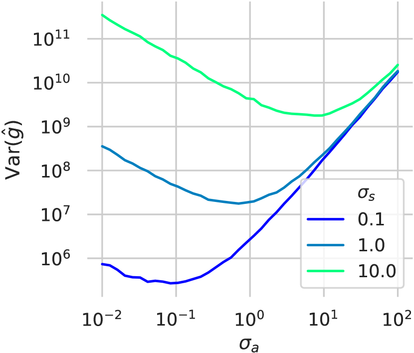
(a) Relationship between $\Sigma_{s}$ and $\Sigma_{a}$

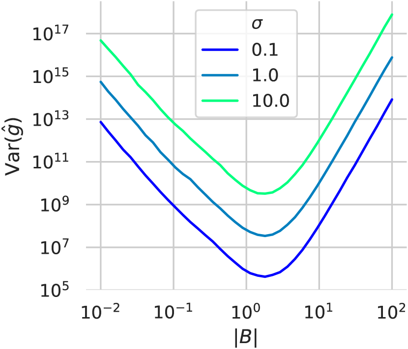
(b) Control authority $|B|$

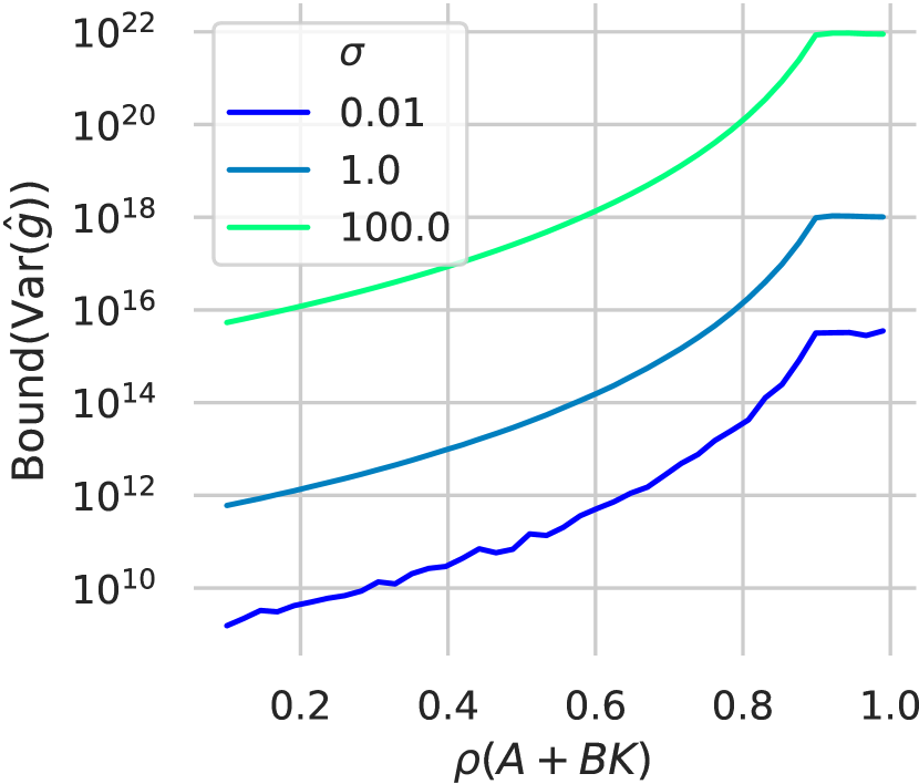
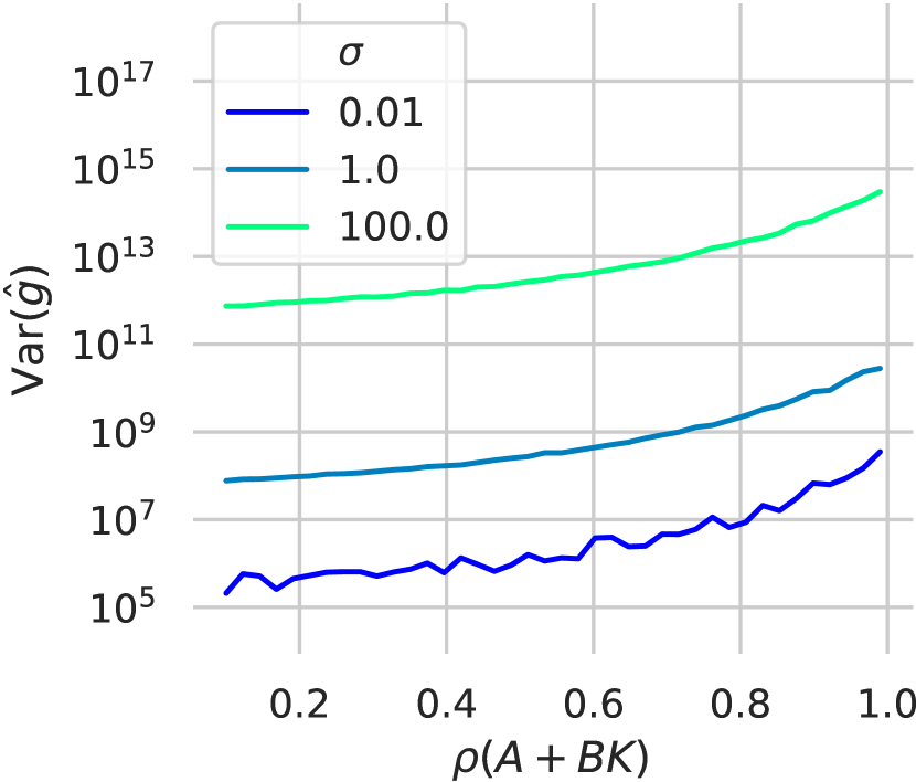
(c) Stability $\rho(A+BK)$

Figure 1: Comparison between our upper bound from Theorem 1 (top) and the empirically measured variance (bottom) as they relate to various parameters of the LQR problem. Behavior is qualitatively similar for action noise covariance (a) and control authority (b), but less similar for the stability (c) where our bounds are loose. Further discussion is in Sections 4, 4 and 2.

In the first set of experiments, we compare our upper bound of $\nu(\hat{g})$ to its empirical value when executing REINFORCE in randomly generated LQR problems. Our results show qualitative similarity in the parameters for which our upper and lower bounds match. On the other hand, the gap with respect to stability-related parameters is also visible. For each experiment shown here, we repeated the experiment with different random seeds and observed qualitatively identical results.

We generate random LQR problems with the following procedure. We sample each entry in $A$ and $B$ i.i.d. from $\mathcal{N}(0,\sigma{=}n^{-1/2})$ and $\mathcal{N}(0,\sigma{=}m^{-1/2})$ respectively. To construct a random $k\times k$ positive definite matrix, we sample from the $\mathrm{Wishart}(k^{-1}I,k)$ distribution by computing $Q=X^{T}X$ for $X$ i.i.d. analogous to $A$. The scale factor $k^{-1}$ ensures that if the vector $x$ is distributed by $\mathcal{N}(0,k^{-1}I)$, such that $\mathbb{E}[\|x\|^{2}]=1$, then $\mathbb{E}[x^{T}Qx]=1$. We sample $Q,R,\Sigma_{s}$, and $\Sigma_{a}$ this way.

In each experiment, we vary some of these parameters systematically while holding the others constant, allowing us to visualize the impact of each parameter on $\nu(\hat{g})$. We plot the upper bound of Theorem 1 on the top row of Figure 1, and the empirical estimate of $\nu(\hat{g})$ on the bottom row. In both cases, since the variance depends on the initial state $s_{1}$, we sample $N=100$ initial states $s_{1}$ from $\mathcal{N}(0,n^{-1}I)$ and plot $\mathbb{E}_{s_{1}\sim\mathcal{N}(0,n^{-1}I)}\nu(\hat{g})$. We estimate $\nu(\hat{g})|_{s_{1}=s}$ for a particular initial state $s$ by sampling $30$ trajectories with random $\epsilon^{a},\ \epsilon^{s}$.

Effect of $\Sigma_{a}$.

In this experiment, we generate a random LQR problem and replace $\Sigma_{a}$ with $\sigma_{a}I$ for $\sigma_{a}$ geometrically spaced in the range $[10^{-2},10^{2}]$. Using a scaled identity matrix is common practice when applying RL to a problem where there is no a priori reason to correlate the noise between different action dimensions. We evaluate the variance at the value $K=K^{\star}$, where $K^{\star}$ is the infinite-horizon optimal controller computed using traditional LQR synthesis, as described in Section 2. Using $K^{\star}$ ensures that $\rho(A+BK)<1$, a required condition to apply Theorem 1.

Results are shown in Figure 1(a). The separate line plots correspond to scaling the random $\Sigma_{s}$ by the values $\{0.1,1,10\}$, while the $x-$axis corresponds to the value of $\sigma_{a}$. For each value of $\sigma_{s}$, there appears to be a unique $\sigma_{a}$ that minimizes $\nu(\hat{g})$, and this value of $\sigma_{a}$ increases with $\sigma_{s}$. This phenomenon appears in both the bound and empirical variance.

Effect of $\|B\|$.

In this experiment, we generate a random problem where $m=n$ and replace $B$ with $bI$ for $b$ geometrically spaced in the range $[10^{-2},10^{2}]$. The resulting system essentially gives the policy direct control over each state. For each $B$, we compute a separate infinite-horizon optimal $K$ and sample the variance for different $s_{1}$. Results are shown in Figure 1(b). The separate line plots correspond to scaling both the random $\Sigma_{s}$ and the random $\Sigma_{a}$ by the values $\{0.1,1,10\}$. The $x-$axis corresponds to the value of $b$. Again, there appears to be a unique $\|B\|$ that minimizes $\nu(\hat{g})$, but its value changes minimally for different magnitudes of $\Sigma_{s},\ \Sigma_{a}$.

Effect of $\rho(A+BK)$.

Figure 2: Scatter plot of empirical $\nu(\hat{g})$ ($x-$axis) and upper bound from Theorem 1 ($y-$axis) with varying state dimensionality $n$ and time horizon $H$. Each point represents one random LQR problem.

Here we measure the change in variance with respect to the closed-loop spectral radius $\rho(A+BK)$. To synthesize controllers $K$ such that $\rho(A+BK)$ obtains a specified value, we use the pole placement algorithm of Tits and Yang (1996). A pole placement algorithm $\mathscr{P}$ is a function

$$K=\mathscr{P}(A,B,\lambda_{1},\dots,\lambda_{n}),\quad\lambda_{i}\in\mathbb{C},$$

such that the eigenvalues of $A+BK$ are $\lambda_{1},\dots,\lambda_{n}$. We sample a “prototype” set of $n$ eigenvalues with $\lambda_{1},\dots,\lambda_{\lceil n/2\rceil}$ as complex conjugate pairs $\lambda_{i},\lambda_{i+1}=re^{\pm i\varphi}$, where ${r\sim\operatorname{Uniform}([0,1])}$ and $\varphi\sim\operatorname{Uniform}([0,\pi))$, and sample the remaining real $\lambda_{i}$ from $\operatorname{Uniform}([-1,1])$. Then, for each desired $\rho$, we compute $K_{\rho}=\mathscr{P}(A,B,\rho\lambda_{1},\dots,\rho\lambda_{n}).$ By rescaling the same set of $\lambda_{i}$ instead of sampling a new set for each $\rho$, we avoid confounding effects from changing other properties of $K$.

Results are shown in Figure 1(c). Again, we repeat the experiment for different magnitudes of $\Sigma_{s}$ and $\Sigma_{a}$. Unlike the previous two experiments, here we see qualitatively different behavior between our upper bound and the empirical variance. The bound begins to increase rapidly near $\rho=1$, corresponding to the growth of $1/(1-\rho)$ in the term $H^{\prime}$, but at $\rho=0.9$ the $H$ term becomes active in $H^{\prime}$, and the bound suddenly flattens. In contrast, the empirical variance grows more moderately and does not explode near the threshold of system instability. This provides further evidence that the upper bound of Theorem 1 can be tightened to match the $\sqrt{H^{\prime}}$ and $\sqrt{H}$ terms in the special-case lower bound of Theorem 2.

Dimensionality parameters.

In all of the preceding experiments, we arbitrarily chose the state and action dimensions ${n=5},\ {m=3}$ and time horizon $H=10$. To visualize the variance for other values of these parameters, we generate $1000$ random LQR problems with $n$ and $H$ each varying over the set $\{3,10,30\}$. We fix $m=\lceil n/2\rceil$. Results are shown in Figure 2. The overall positive trend with a slope greater than $1$ shows that the bound grows superlinearly with respect to the empirical, as expected. One interesting property is the tighter clustering for large values of $n$. This may be due to several eigenvalue distribution results in random matrix theory which state that, as $n\to\infty$, our random LQR problems tend to become similar up to a basis change (Tao, 2012).

4.1 RL learning curves for varying $\Sigma_{a}$

The results in Section 4 suggest that, for a fixed $\Sigma_{s}$, the magnitude of $\Sigma_{a}$ has a significant effect on $\nu(g)$. This is of practical interest because $\Sigma_{a}$ is usually under control of the RL practitioner. It is therefore natural to ask if the change in variance corresponds to a change in the rate of convergence of REINFORCE. We test this empirically by executing REINFORCE in variants of one random LQR problem with different values of $\Sigma_{a}$ and $\Sigma_{s}$. To avoid a confounding effect from larger $\Sigma_{a}$ incurring greater penalty from the $-a_{t}^{T}Ra_{t}$ term in $r_{t}$, we evaluate the trained policies in a modified version of the problem where $\Sigma_{a}=\Sigma_{s}=\mathbf{0}$. As discussed in Section 2, the optimal $K^{\star}$ for the stochastic problem is also optimal for the deterministic problem, so each problem variant should converge to the same evaluation returns in the limit.

We initialize $K$ by perturbing the elements of the LQR-optimal controller with i.i.d. Gaussian noise and scaling the perturbation until $\rho(A+BK)\approx 0.98$. After every $10$ iterations of REINFORCE, we evaluate the current policy in the noise-free environment. For each $(\Sigma_{a},\Sigma_{s})$ pair, we repeat this experiment $10$ times with different random seeds. The random seed only affects the $\epsilon^{a}_{t},\epsilon^{s}_{t}$ and $s_{1}$ samples. The aggregate data are shown in Figure 3. Shaded bands correspond to one standard deviation across the separate runs of REINFORCE. The lowercase $\sigma_{a},\sigma_{s}$ refer to scaling factors applied to the initial samples of $\Sigma_{a},\Sigma_{s}$ in the random LQR problem.

The effect is quite different than one would predict from variance alone. For all values of $\Sigma_{s}$ in the experiment, problems with larger $\Sigma_{a}$ converge faster—whereas Figure 1(a) would suggest that the “optimal” value of $\Sigma_{a}$ changes with respect to $\Sigma_{s}$. The fact that larger $\Sigma_{a}$ tends to make REINFORCE converge faster is not obvious, given the $\Sigma_{a}^{-1}$ term in $\hat{g}$ (6). Also, when $\Sigma_{a}$ is very small and $\Sigma_{s}$ is very large, the algorithm becomes unstable and sees large variations across different random seeds. For the middle values $\Sigma_{a}\in\{0.1,1.0\}$, we observe that larger $\Sigma_{s}$ causes faster convergence.

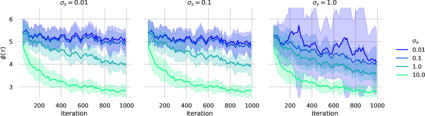
Figure 3: Learning curves of REINFORCE for a random LQR problem with varying scales of action noise $\sigma_{a}$ and environment noise $\sigma_{s}$. Larger $\sigma_{a}$ strictly improves learning, despite larger variance of $\hat{g}$.

5 Discussion

In this work, we derived bounds on the variance of the REINFORCE policy gradient estimator in the stochastic linear-quadratic control setting. Our upper bound is fully general, while our lower bound applies to the scalar case at a stationary point. The bounds match with respect to all system parameters except the time horizon $H$ and stability $\rho(A+BK)$. We compared our bound prediction to the empirical variance in a variety of experimental settings, finding a close qualitative match in the parameters for which the bounds are tight.

Our experiments in Section 4.1 plotting the empirical convergence rate of REINFORCE suggest that the effect of action noise $\Sigma_{a}$ on the overall RL performance is not fully captured by its effect on the variance. An interesting direction for future work would be to investigate the role of $\Sigma_{a}$ more closely and attempt to disentangle its effect on gradient magnitude, variance, exploration, and regularization. Such an analysis could lead to improved variance reduction methods or algorithms that manipulate $\Sigma_{a}$ to speed up the RL optimization.

Acknowledgements

The authors thank Gaurav S. Sukhatme and Fei Sha for their discussions regarding this work.

Appendix A Proof of Theorem 1

In this appendix, we provide the detailed derivation of the upper bound stated in Theorem 1. We define the following notations: let $\delta^{s}_{t}$ and $\delta_{t}^{a}$ be independent random vectors that follow $\mathcal{N}(\mathbf{0},I_{n})$ and $\mathcal{N}(\mathbf{0},I_{m})$ respectively for all $t$. The $\epsilon^{s}_{t}$ and $\epsilon^{a}_{t}$ defined in Equations 3 and 5 are thus written as $\epsilon^{s}_{t}=\Sigma_{s}^{\frac{1}{2}}\delta^{s}_{t}$ and $\epsilon^{a}_{t}=\Sigma_{a}^{\frac{1}{2}}\delta^{a}_{t}$. We will use the following steps to upper-bound $\mathbb{E}\left[\operatorname{\mathbf{tr}}({\hat{g}^{\top}\hat{g}})\right]$:

1. Bound $\operatorname{\mathbf{tr}}({\hat{g}^{\top}\hat{g}})$ by $P$, a polynomial of ${d^{s}_{t}\triangleq\|\delta^{s}_{t}\|}$ and ${d^{a}_{t}\triangleq\|\delta^{a}_{t}\|}$ for ${t=1,2,\ldots,H}$. We restrict that $P$ should have only nonnegative coefficients. Since we assume $\delta_{t}^{s}$ and $\delta_{t}^{a}$ are independent random vectors with standard normal distribution, $d^{s}_{t}$ and $d^{a}_{t}$ will be independent random variables following the $\chi(n)$ and $\chi(m)$ distributions respectively.

2. Bound the sum of the (already nonnegative) coefficients of $P$ by substituting all of the $d^{s}_{t},\ d^{a}_{t}$ with one. More formally, let

   $$P(\{d_{t}^{s},d_{t}^{a}\}_{t=1}^{H})=\sum_{i}C_{i}\prod_{t=1}^{H}(d_{t}^{s})^{\alpha_{t,i}}\prod_{t=1}^{H}(d_{t}^{a})^{\beta_{t,i}},$$

   where $\prod_{t=1}^{H}(d_{t}^{a})^{\alpha_{t,i}}\prod_{t=1}^{H}(d_{t}^{s})^{\beta_{t,i}}$ is the $i$-th monomial in $P$, and $C_{i}$ is its nonegative coefficient. Then we calculate $\sum_{i}C_{i}$ by substituting all $d_{t}^{s},d_{t}^{a}$ with $1$. We use the notation $\mathbbm{1}(P)$ to denote this operation (we define the $\mathbbm{1}(\cdot)$ operator analogously for expressions other than $P$ itself):

   $$\mathbbm{1}(P)=P|_{d_{t}^{s}=1,d_{t}^{a}=1,\forall t}=\sum_{i}C_{i}.$$

3. Bound for the expectation of all monomials in $P$, i.e., find $M$ such that

   $$\mathbb{E}\left[\prod_{t=1}^{H}(d_{t}^{s})^{\alpha_{t,i}}\prod_{t=1}^{H}(d_{t}^{a})^{\beta_{t,i}}\right]\leq M,\quad\forall i.$$

With the three steps above, we can then bound $\mathbb{E}\left[\operatorname{\mathbf{tr}}({\hat{g}^{\top}\hat{g}})\right]\leq\mathbb{E}[P]\leq\sum_{i}C_{i}M=M\mathbbm{1}(P)$. To calculate $M$, we can use the known formula for the $k$-th moment of a $\chi$ random variable.

Recall that

$$\hat{g}=\left(\sum_{t=1}^{H}\Sigma_{a}^{-1}\epsilon_{t}^{a}s_{t}^{\top}\right)\left(\sum_{t=1}^{H}r_{t}\right),$$

and thus

$$\operatorname{\mathbf{tr}}({\hat{g}^{\top}\hat{g}})=\underbrace{\operatorname{\mathbf{tr}}\left[\left(\sum_{t=1}^{H}\Sigma_{a}^{-1}\epsilon^{a}_{t}s_{t}^{\top}\right)^{\top}\left(\sum_{t=1}^{H}\Sigma_{a}^{-1}\epsilon^{a}_{t}s_{t}^{\top}\right)\right]}_{\textbf{{Term}}_{1}}\underbrace{\left(\sum_{t=1}^{H}r_{t}\right)^{2}}_{\textbf{{Term}}_{2}}.$$

Thanks to the property $\mathbbm{1}(P)=\mathbbm{1}(P_{1})\mathbbm{1}(P)$ for polynomial $P\equiv P_{1}P$, and $\mathbbm{1}(P)=\mathbbm{1}(P_{1})+\mathbbm{1}(P)$ for $P\equiv P_{1}+P$, we do not need to directly find $P$ and bound $\mathbbm{1}(P)$. Instead, we can bound $\mathbbm{1}(P^{\prime})$ for some smaller-order component $P^{\prime}$ of $P$, and then using the above addition/multiplication operations to obtain $\mathbbm{1}(P)$. Below in Section A.1, we first bound $\|s_{t}\|$ by a polynomial $\lceil s_{t}\rceil$ of $\{d_{\tau}^{s},d_{\tau}^{a}\}$, and then find $\mathbbm{1}(\lceil s_{t}\rceil)$. In Section A.2 and A.3, we further upper bound $\mathbbm{1}(\textbf{{Term}}_{1})$ and $\mathbbm{1}(\textbf{{Term}}_{2})$ with the help of $\mathbbm{1}(\lceil s_{t}\rceil)$. Then finally we obtain an upper bound for $\mathbb{E}[\operatorname{\mathbf{tr}}({\hat{g}^{\top}\hat{g}})]$ as $M\mathbbm{1}(\textbf{{Term}}_{1})\mathbbm{1}(\textbf{{Term}}_{2})$.

A.1 Bounding $\|s_{t}\|$

In this section, we bound $\|s_{t}\|$ from above. Although the spectral radius $\rho(A+BK)$ determines the asymptotic stability of the closed-loop system, it guarantees little about the transient behavior–for example, for any $x>1$ and $0<\epsilon<1$, the matrix

$$A=\begin{bmatrix}\epsilon&x\\ 0&\epsilon\end{bmatrix}$$

has the properties $\rho(A)<1,\ \|A\|>x$. Therefore, while the state magnitude $\|s_{t}\|$ is bounded by the operator norm $\|A+BK\|^{t-1}$, it is too restrictive to require $\|A+BK\|<1$. Instead, we will use the following result from the literature:

Lemma 3 (Trefethen and Embree (2005)).

Let $A\in\mathbb{R}^{n\times n}$ be a matrix with $\rho(A)<1$. Then there exists $\mu>0$ such that, for all $k\in\mathbb{N}$,

$$\|A^{k}\|\leq\mu\rho(A)^{k}.$$ (7)

$\mu$ is bounded by the “resolvent condition” $\mu\leq 2enr(A)$, where $e$ is the exponential constant and

$$r(A)=\sup_{z\in\mathbb{C},\ |z|>1}(|z|-1)\|(zI-A)^{-1}\|.$$ (8)

The derivation and interpretation of (8) is a deep subject related to the matrix pseudospectrum, covered extensively by Trefethen and Embree (2005). Intuitively, $r(A)$ is large if a small perturbation $\epsilon\in\mathbb{R}^{n\times n}$ would cause $\rho(\epsilon+A)>1$.

Expanding the state transition function in Equation 3 with the linear stochastic policy in Equation 5, we get

$$s_{t}=(A+BK)^{t-1}s_{1}+\sum_{\tau=1}^{t-1}(A+BK)^{t-\tau-1}(\Sigma_{s}^{\frac{1}{2}}\delta^{s}_{\tau}+B\Sigma_{a}^{\frac{1}{2}}\delta^{a}_{\tau}).$$ (9)

Recall that $\|\cdot\|$ denotes the $\ell_{2}$ norm for vectors and the $\ell_{2}-\ell_{2}$ operator norm for matrices. By Lemma 3, there exists $\mu$ such that $\|(A+BK)^{k}\|\leq\mu\rho(A)^{k}$. Let $f=\rho(A+BK)$, $\sigma_{s}^{2}=\|\Sigma_{s}\|$, $\sigma_{a}^{2}=\|\Sigma_{a}\|$, and $b=\|B\|$. By repeatedly applying the triangle inequality,

$$\begin{split}\|s_{t}\|&=\left\|(A+BK)^{t-1}s_{1}+\sum_{\tau=1}^{t-1}(A+BK)^{t-\tau-1}(\Sigma_{s}^{\frac{1}{2}}\delta^{s}_{\tau}+B\Sigma_{a}^{\frac{1}{2}}\delta^{a}_{\tau})\right\|\\ &\leq\left\|(A+BK)^{t-1}s_{1}\right\|+\sum_{\tau=1}^{t-1}\left\|(A+BK)^{t-\tau-1}(\Sigma_{s}^{\frac{1}{2}}\delta^{s}_{\tau}+B\Sigma_{a}^{\frac{1}{2}}\delta^{a}_{\tau})\right\|\\ &\leq\mu f^{t-1}\|s_{1}\|+\mu\sum_{\tau=1}^{t-1}f^{t-\tau-1}(\sigma_{s}d^{s}_{\tau}+b\sigma_{a}d^{a}_{\tau}).\end{split}$$ (10)

We denote the final bound in (10) as $\lceil s_{t}\rceil$. The bound $\lceil s_{t}\rceil$ is linear in the random variables $\{d^{s}_{t},d^{a}_{t}\}_{t=1}^{H}$ with only positive coefficients. Furthermore,

$$\begin{split}\mathbbm{1}(\lceil s_{t}\rceil)&=\mu f^{t-1}\|s_{1}\|+\mu\sum_{\tau=1}^{t-1}f^{t-\tau-1}(\sigma_{s}+b\sigma_{a})\\ &=\mu f^{t-1}\|s_{1}\|+\mu\sum_{\tau=0}^{t-2}f^{\tau}(\sigma_{s}+b\sigma_{a}).\end{split}$$ (11)

A.2 Bounding $\textbf{{Term}}_{1}$

Lemma 4.

$$\operatorname{\mathbf{tr}}\left[\left(\sum_{t=1}^{H}\Sigma_{a}^{-1}\epsilon^{a}_{t}s_{t}^{\top}\right)^{\top}\left(\sum_{t=1}^{H}\Sigma_{a}^{-1}\epsilon^{a}_{t}s_{t}^{\top}\right)\right]\leq\|\Sigma_{a}^{-1}\|\left(\sum_{t=1}^{H}d^{a}_{t}\|s_{t}\|\right)^{2}.$$

Proof.

Let $\xi_{t}=\Sigma_{a}^{-1}\epsilon^{a}_{t}$. Then

$$\begin{split}\operatorname{\mathbf{tr}}\left[\left(\sum_{t=1}^{H}\xi_{t}s_{t}^{\top}\right)^{\top}\left(\sum_{t=1}^{H}\xi_{t}s_{t}^{\top}\right)\right]&=\operatorname{\mathbf{tr}}\left[\sum_{1\leq i,j\leq H}s_{i}\xi_{i}^{\top}\xi_{j}s_{j}^{\top}\right]\\ &=\sum_{1\leq i,j\leq H}\xi_{i}^{\top}\xi_{j}s_{i}^{\top}s_{j}\\ &\leq\sum_{1\leq i,j\leq H}|\xi_{i}^{\top}\xi_{j}||s_{i}^{\top}s_{j}|\\ &=\sum_{1\leq i,j\leq H}|{\delta^{a}_{i}}^{\top}\Sigma_{a}^{-1}\delta^{a}_{j}||s_{i}^{\top}s_{j}|\\ &\leq\sum_{1\leq i,j\leq H}\|\Sigma_{a}^{-1}\|\|\delta^{a}_{i}\|\|\delta^{a}_{j}\|\|s_{i}\|\|s_{j}\|\\ &=\|\Sigma_{a}^{-1}\|\left(\sum_{t=1}^{H}\|\delta^{a}_{t}\|\|s_{t}\|\right)^{2}\\ &\leq\|\Sigma_{a}^{-1}\|\left(\sum_{t=1}^{H}d_{t}^{a}\lceil s_{t}\rceil\right)^{2},\end{split}$$ (12)

in which we make use of the Cauchy-Schwarz inequality and the fact that $\Sigma^{{\frac{1}{2}}}\Sigma^{-2}\Sigma^{{\frac{1}{2}}}=\Sigma^{-1}$ for positive semidefinite $\Sigma$. ∎

A.3 Bounding $\textbf{{Term}}_{2}$

We now bound $C\triangleq\sum_{t=1}^{H}-r_{t}$ from above. Note that $-r_{t}\geq 0$, since $Q\succeq 0$ and $R\succ 0$. Let $q=\|Q\|$, $r=\|R\|$, and $k=\|K\|$. Then

$$\begin{split}C=\sum_{t=1}^{H}-r_{t}&=\sum_{t=1}^{H}s_{t}^{\top}Qs_{t}+a_{t}^{\top}Ra_{t}\\ &\leq\sum_{t=1}^{H}q\|s_{t}\|^{2}+r\|a_{t}\|^{2}=\sum_{t=1}^{H}q\|s_{t}\|^{2}+r\|Ks_{t}+\Sigma_{a}^{\frac{1}{2}}\delta^{a}_{t}\|^{2}\\ &\leq\sum_{t=1}^{H}q\|s_{t}\|^{2}+r(k\|s_{t}\|+\sigma_{a}\|\delta^{a}_{t}\|)^{2}\\ &\leq\sum_{t=1}^{H}q\|s_{t}\|^{2}+2rk^{2}\|s_{t}\|^{2}+2r\sigma_{a}^{2}\|\delta^{a}_{t}\|^{2}\\ &\leq(q+2rk^{2})\sum_{t=1}^{H}\lceil s_{t}\rceil^{2}+2r\sigma_{a}^{2}\sum_{t=1}^{H}(d^{a}_{t})^{2},\end{split}$$ (13)

where the triangle inequality and the fact $(a+b)^{2}\leq 2(a^{2}+b^{2})$ are used above. This bound on $C$ is a quadratic polynomial in the $d^{s},d^{a}$.

A.4 Combining bounds

Combining Section A.2 and Section A.3, we have

$$\begin{split}\operatorname{\mathbf{tr}}({\hat{g}^{\top}\hat{g}})\leq P=C^{2}\|\Sigma_{a}^{-1}\|\left(\sum_{t=1}^{H}d^{a}_{t}\lceil s_{t}\rceil\right)^{2}.\end{split}$$ (14)

For brevity, let $\alpha=\|\Sigma_{a}^{-1}\|$, $\beta=q+2rk^{2}$, $\gamma=2r\sigma_{a}^{2}$, $\sigma=\sigma_{s}+b\sigma_{a}$, and $H^{\prime}\triangleq\min\left\{H,\frac{1}{1-f}\right\}$. $H^{\prime}$ reflects the stability of the closed-loop system: if highly stable ($f\ll 1$), we have $H^{\prime}\ll H$, but when approaching instability ($f\to 1$), $H^{\prime}$ approaches $H$.

We expand $P$ and substitute $d^{s}_{t}=1,\ d^{a}_{t}=1$ for all $t$ to compute the sum of $P$’s coefficients, using the notation $\mathbbm{1}(\cdot)$ for the transformation of replacing all $d$ with $1$. We first bound $\mathbbm{1}(C^{2})$:

$$\begin{split}\mathbbm{1}(C^{2})\leq\left(\gamma H+\beta\sum_{t=1}^{H}\mathbbm{1}(\lceil s_{t}\rceil)^{2}\right)^{2}&\leq\left(\gamma H+\beta\mu^{2}\sum_{t=1}^{H}\left[f^{t-1}\|s_{1}\|+\sigma H^{\prime}\right]^{2}\right)^{2}\\ &\leq\left(\gamma H+2\beta\mu^{2}\sum_{t=1}^{H}\left[f^{2t-2}\|s_{1}\|^{2}+\sigma^{2}H^{\prime 2}\right]\right)^{2}\\ &\leq\left(\gamma H+2\beta\mu^{2}(H^{\prime}\|s_{1}\|^{2}+\sigma^{2}HH^{\prime 2})\right)^{2}\\ \end{split}$$ (15)

where the result is obtained by repeatedly applying the fact $(a+b)^{2}\leq 2(a^{2}+b^{2})$. Next,

$$\begin{split}\mathbbm{1}(\left(\sum_{t=1}^{H}d^{a}_{t}\lceil s_{t}\rceil\right)^{2})&\leq\left(\mu\sum_{t=1}^{H}f^{t-1}\|s_{1}\|+\sigma H^{\prime}\right)^{2}\\ &\leq\mu^{2}H^{\prime 2}(\|s_{1}\|+\sigma H)^{2}.\\ \end{split}$$ (16)

Finally,

$$\begin{split}\mathbbm{1}(P)&\leq\alpha\mu^{2}H^{\prime 2}\left(\gamma H+2\beta\mu^{2}(H^{\prime}\|s_{1}\|^{2}+\sigma^{2}HH^{\prime 2})\right)^{2}(\|s_{1}\|+\sigma H)^{2}\\ &=4\|\Sigma_{a}^{-1}\|\mu^{2}H^{\prime 2}\left(r\sigma_{a}^{2}H+\mu^{2}(q+2rk^{2})(H^{\prime}\|s_{1}\|^{2}+\sigma^{2}HH^{\prime 2})\right)^{2}(\|s_{1}\|+\sigma H)^{2}\\ &\triangleq\overline{\mathbbm{1}(P)}.\end{split}$$ (17)

$\overline{\mathbbm{1}(P)}$ is an order-8 polynomial in the $d^{s},d^{a}$. The formula for the 8th moment of a $\chi(n)$ random variable is

$$\mathbb{E}[X^{8}]=n(n+2)(n+4)(n+6),$$

so $\mathbb{E}[\operatorname{\mathbf{tr}}({\hat{g}^{\top}\hat{g}})]\leq\overline{\mathbbm{1}(P)}\cdot O(\bar{n}^{4})$, where $\bar{n}=\max(n,m)$.

(Since we are summing the variances of $O(\bar{n}^{2})$ random variables in $\hat{g}$, we would expect scaling of no less than $\bar{n}^{2}$ compared to the scalar case.)

Appendix B $\mathbb{E}[\hat{g}^{2}]$’s lower bound in the scalar case

In this section, we make the assumption that $m=n=1$, i.e., the states and actions are both scalars. The matrices $A,B,K,Q,R$ are thus denoted as $a,b,k,q,r$ here (notice that this notation $r$ is different from the notation $r_{t}$ for reward). Other notations follow the definitions in Appendix A. The aim in this appendix is to derive a lower bound for $\mathbb{E}[\hat{g}^{2}]$ in the special case when $0\leq a+bk<1$.

Lemma 5.

$$\mathbb{E}\left[\left(\sum_{t=1}^{H}\frac{\epsilon_{t}^{a}s_{t}}{\sigma_{a}^{2}}\right)^{2}\left(\sum_{t=1}^{H}r_{t}\right)^{2}\right]\geq\mathbb{E}\left[\left(\sum_{t=1}^{H}\frac{\epsilon_{t}^{a}s_{t}}{\sigma_{a}^{2}}\right)^{2}\right]\mathbb{E}\left[\left(\sum_{t=1}^{H}r_{t}\right)^{2}\right].$$ (18)

Proof.

When $a+bk\geq 0$, all terms have positive coefficients. Rename the $2H$ random variables $\{\delta_{t}^{s},\delta_{t}^{a}\}_{t=1}^{H}$ as $x_{1},\ldots,x_{2H}$. We can see that a monomial on the right-hand side:

$$\mathbb{E}\big{[}x_{1}^{\alpha_{1}}\cdots x_{2H}^{\alpha_{2H}}\big{]}\mathbb{E}\big{[}x_{1}^{\beta_{1}}\cdots x_{2H}^{\beta_{2H}}\big{]}$$

corresponds to the monomial on the left-hand side:

$$\mathbb{E}\big{[}x_{1}^{\alpha_{1}+\beta_{1}}\cdots x_{2H}^{\alpha_{2H}+\beta_{2H}}\big{]}.$$

The $x_{i}$ are independent zero-mean normal random variables, so the property $\mathbb{E}[x_{i}^{\alpha}]\mathbb{E}[x_{i}^{\beta}]\leq\mathbb{E}[x_{i}^{\alpha+\beta}]$ holds for any non-negative integers $\alpha,\beta$. Combining with the fact that all coefficients are non-negative shows the lemma. ∎

In the following two subsections, we lower bound the two terms on the right-hand side of Eq. (18) separately. Note that the first term can be simplified as

$$\left(\sum_{t=1}^{H}\frac{\epsilon_{t}^{a}s_{t}}{\sigma_{a}^{2}}\right)^{2}=\left(\sum_{t=1}^{H}\frac{\delta_{t}^{a}s_{t}}{\sigma_{a}}\right)^{2}=\frac{1}{\sigma_{a}^{2}}\left(\sum_{t=1}^{H}\delta_{t}^{a}s_{t}\right)^{2}.$$

B.1 Lower bounding $\mathbb{E}\left[\left(\sum_{t=1}^{H}\delta_{t}^{a}s_{t}\right)^{2}\right]$

By the expansion of $s_{t}$ in Eq. (9), we have

$$\mathbb{E}\left[\left(\sum_{t=1}^{H}\delta_{t}^{a}s_{t}\right)^{2}\right] =\mathbb{E}\left[\left(\sum_{t=1}^{H}\delta_{t}^{a}\left((a+bk)^{t-1}s_{1}+L_{t}\right)\right)^{2}\right]$$

$$\geq\mathbb{E}\left[\left(\sum_{t=1}^{H}\delta_{t}^{a}(a+bk)^{t-1}s_{1}\right)^{2}\right]+\mathbb{E}\left[\left(\sum_{t=1}^{H}\delta_{t}^{a}L_{t}\right)^{2}\right],$$

where $L_{t}\triangleq\sum_{\tau=1}^{t-1}(a+bk)^{t-1-\tau}(\sigma_{s}\delta_{\tau}^{s}+b\sigma_{a}\delta_{\tau}^{a})$. The first term is equal to $\sum_{t=1}^{H}(a+bk)^{2t-2}s_{1}^{2}=\frac{1-(a+bk)^{2H}}{1-(a+bk)^{2}}s_{1}^{2}$. The second term can be further written as

$$\mathbb{E}\left[\left(\sum_{t=1}^{H}\delta_{t}^{a}\sum_{\tau=1}^{t-1}(a+bk)^{t-1-\tau}(\sigma_{s}\delta_{\tau}^{s}+b\sigma_{a}\delta_{\tau}^{a})\right)^{2}\right]$$

$$=\mathbb{E}\left[\sum_{t=1}^{H}(\delta_{t}^{a})^{2}\left(\sum_{\tau=1}^{t-1}(a+bk)^{t-1-\tau}(\sigma_{s}\delta_{\tau}^{s}+b\sigma_{a}\delta_{\tau}^{a})\right)^{2}\right]$$

$$=\mathbb{E}\left[\sum_{t=1}^{H}\left(\sum_{\tau=1}^{t-1}(a+bk)^{t-1-\tau}(\sigma_{s}\delta_{\tau}^{s}+b\sigma_{a}\delta_{\tau}^{a})\right)^{2}\right]$$

$$=\mathbb{E}\left[\sum_{t=1}^{H}\sum_{\tau=1}^{t-1}(a+bk)^{2t-2-2\tau}(\sigma_{s}^{2}+b^{2}\sigma_{a}^{2})\right]$$

$$=(\sigma_{s}^{2}+b^{2}\sigma_{a}^{2})\mathbb{E}\left[\sum_{t=1}^{H}\frac{1-(a+bk)^{2t-2}}{1-(a+bk)^{2}}\right]$$

$$=(\sigma_{s}^{2}+b^{2}\sigma_{a}^{2})\left(\frac{H}{1-(a+bk)^{2}}-\frac{1-(a+bk)^{2H}}{(1-(a+bk)^{2})^{2}}\right).$$

In the above several equalities, we use the independence among $\delta_{t}^{a},\delta_{t}^{s}$. Combining two terms, we get

$$\mathbb{E}\left[\left(\sum_{t=1}^{H}\delta_{t}^{a}s_{t}\right)^{2}\right] \geq\frac{s_{1}^{2}+H(\sigma_{s}^{2}+b^{2}\sigma_{a}^{2})}{1-(a+bk)^{2}}-\frac{(a+bk)^{2H}}{1-(a+bk)^{2}}s_{1}^{2}-(\sigma_{s}^{2}+b^{2}\sigma_{a}^{2})\frac{1-(a+bk)^{2H}}{(1-(a+bk)^{2})^{2}}$$

$$=\left(\frac{1-(a+bk)^{2H}}{1-(a+bk)^{2}}s_{1}^{2}+\left(H-\frac{1-(a+bk)^{2H}}{1-(a+bk)^{2}}\right)\frac{\sigma_{s}^{2}+b^{2}\sigma_{a}^{2}}{1-(a+bk)^{2}}\right)$$

$$\approx\begin{cases}\frac{s_{1}^{2}+H(\sigma_{s}^{2}+b^{2}\sigma_{a}^{2})}{1-(a+bk)^{2}}&\text{when\ }H\gg\frac{1}{1-(a+bk)^{2}}\\ H\left(s_{1}^{2}+H(\sigma_{s}^{2}+b^{2}\sigma_{a}^{2})\right)&\text{when\ }H\ll\frac{1}{1-(a+bk)^{2}}\end{cases}$$

$$\approx\min\left\{H,\frac{1}{1-(a+bk)^{2}}\right\}\left(s_{1}^{2}+H(\sigma_{s}^{2}+b^{2}\sigma_{a}^{2})\right)$$

$$\approx H^{\prime}\left(s_{1}^{2}+H(\sigma_{s}^{2}+b^{2}\sigma_{a}^{2})\right).$$

B.2 Lower bounding $\mathbb{E}\left[\left(\sum_{t=1}^{H}r_{t}\right)^{2}\right]$

We first lower bound this term by

$$\mathbb{E}\left[\left(\sum_{t=1}^{H}r_{t}\right)^{2}\right] \geq\mathbb{E}\left[\sum_{t=1}^{H}r_{t}\right]^{2}=\mathbb{E}\left[\sum_{t=1}^{H}qs_{t}^{2}+r(ks_{t}+\sigma_{a}\delta_{t}^{a})^{2}\right]^{2}$$

$$=\mathbb{E}\left[\sum_{t=1}^{H}(q+rk^{2})s_{t}^{2}+2rks_{t}\sigma_{a}\delta_{t}^{a}+r\sigma_{a}^{2}\delta_{t}^{a2}\right]^{2}$$

$$=\left((q+rk^{2})\mathbb{E}\left[\sum_{t=1}^{H}s_{t}^{2}\right]+Hr\sigma_{a}^{2}\right)^{2}$$

$$\mathbb{E}\left[\sum_{t=1}^{H}s_{t}^{2}\right] =\mathbb{E}\left[\sum_{t=1}^{H}\left((a+bk)^{t-1}s_{1}+L_{t}\right)^{2}\right]$$

$$=\mathbb{E}\left[\sum_{t=1}^{H}\left((a+bk)^{2t-2}s_{1}^{2}+2(a+bk)^{t-1}s_{1}L_{t}+L_{t}^{2}\right)\right]$$

$$=\mathbb{E}\left[\sum_{t=1}^{H}(a+bk)^{2t-2}s_{1}^{2}+\sum_{t=1}^{H}\left(\sum_{\tau=1}^{t-1}(a+bk)^{t-1-\tau}(\sigma_{s}\delta_{t}^{s}+b\sigma_{a}\delta_{t}^{a})\right)^{2}\right] \mathbb{E}[(a+bk)^{t-1}s_{1}L_{t}] L_{t}$$ (the middle term is zero because is a sum of zero-mean RVs)

$$=\frac{1-(a+bk)^{2H}}{1-(a+bk)^{2}}s_{1}^{2}+\mathbb{E}\left[\sum_{t=1}^{H}\sum_{\tau=1}^{t-1}(a+bk)^{2t-2-2\tau}(\sigma_{2}^{2}+b^{2}\sigma_{a}^{2})\right]$$

$$=\frac{1-(a+bk)^{2H}}{1-(a+bk)^{2}}s_{1}^{2}+(\sigma_{s}^{2}+b^{2}\sigma_{a}^{2})\left(\frac{H}{1-(a+bk)^{2}}-\frac{1-(a+bk)^{2H}}{(1-(a+bk)^{2})^{2}}\right)$$

$$\approx\min\left\{H,\frac{1}{1-(a+bk)^{2}}\right\}\left(s_{1}^{2}+H(\sigma_{s}^{2}+b^{2}\sigma_{a}^{2})\right)$$

$$\approx H^{\prime}\left(s_{1}^{2}+H(\sigma_{s}^{2}+b^{2}\sigma_{a}^{2})\right).$$

The second-to-last approximation is obtained similarly as in the previous subsection.

B.3 Combining

Combining the results in previous two subsections, we get the final lower bound on $\mathbb{E}[\hat{g}^{2}]$:

$$\mathbb{E}[\hat{g}^{2}] =\mathbb{E}\left[\left(\sum_{t=1}^{H}\frac{\delta_{t}^{a}s_{t}}{\sigma_{a}}\right)^{2}\left(\sum_{t=1}^{H}r_{t}\right)^{2}\right]\geq\mathbb{E}\left[\left(\sum_{t=1}^{H}\frac{\delta_{t}^{a}s_{t}}{\sigma_{a}}\right)^{2}\right]\mathbb{E}\left[\left(\sum_{t=1}^{H}r_{t}\right)^{2}\right]$$

$$\geq\Omega(c_{1}^{2}c_{2}^{2}),$$

where (recall $\sigma\triangleq\sigma_{s}+b\sigma_{a}$)

$$c_{1} =\frac{1}{\sigma_{a}}\left(|s_{1}|+\sigma\sqrt{H}\right)\sqrt{H^{\prime}},$$

$$c_{2} =r\sigma_{a}^{2}H+(q+rk^{2})(s_{1}^{2}+\sigma^{2}H)H^{\prime}.$$

References

- Duan et al. (2016) Yan Duan, Xi Chen, Rein Houthooft, John Schulman, and Pieter Abbeel. Benchmarking deep reinforcement learning for continuous control. CoRR, abs/1604.06778, 2016.
- Fazel et al. (2018) Maryam Fazel, Rong Ge, Sham M Kakade, and Mehran Mesbahi. Global convergence of policy gradient methods for linearized control problems. CoRR, abs/1801.05039, 2018.
- Greensmith et al. (2004) Evan Greensmith, Peter L Bartlett, and Jonathan Baxter. Variance reduction techniques for gradient estimates in reinforcement learning. Journal of Machine Learning Research, 5(Nov):1471–1530, 2004.
- Kwakernaak and Sivan (1972) Huibert Kwakernaak and Raphael Sivan. Linear optimal control systems, volume 1. Wiley-Interscience New York, 1972.
- Levine (2018) Sergey Levine. Reinforcement learning and control as probabilistic inference: Tutorial and review. CoRR, abs/1805.00909, 2018.
- Malik et al. (2018) Dhruv Malik, Ashwin Pananjady, Kush Bhatia, Koulik Khamaru, Peter L. Bartlett, and Martin J. Wainwright. Derivative-free methods for policy optimization: Guarantees for linear quadratic systems. CoRR, abs/1812.08305, 2018.
- Recht (2018) Benjamin Recht. A tour of reinforcement learning: The view from continuous control. CoRR, abs/1806.09460, 2018.
- Schulman et al. (2015) John Schulman, Sergey Levine, Pieter Abbeel, Michael I. Jordan, and Philipp Moritz. Trust region policy optimization. In ICML, volume 37 of JMLR Workshop and Conference Proceedings, pages 1889–1897. JMLR.org, 2015.
- Schulman et al. (2017) John Schulman, Filip Wolski, Prafulla Dhariwal, Alec Radford, and Oleg Klimov. Proximal policy optimization algorithms. CoRR, abs/1707.06347, 2017.
- Sutton and Barto (2018) Richard S. Sutton and Andrew G. Barto. Reinforcement learning - an introduction. Adaptive computation and machine learning. MIT Press, 2 edition, 2018.
- Tao (2012) Terence Tao. Topics in random matrix theory. Graduate studies in mathematics. American Mathematical Society, Providence, RI, 2012. URL http://cds.cern.ch/record/2122643.
- Tits and Yang (1996) André L Tits and Yaguang Yang. Globally convergent algorithms for robust pole assignment by state feedback. IEEE Transactions on Automatic Control, 41(10):1432–1452, 1996.
- Trefethen and Embree (2005) Lloyd N Trefethen and Mark Embree. Spectra and pseudospectra: The Behavior of Nonnormal Matrices and Operators. Princeton University Press, 2005.
- Tropp (2015) Joel A. Tropp. An introduction to matrix concentration inequalities. Foundations and Trends in Machine Learning, 8(1-2):1–230, 2015.
- Tu and Recht (2018) Stephen Tu and Benjamin Recht. The gap between model-based and model-free methods on the linear quadratic regulator: An asymptotic viewpoint. CoRR, abs/1812.03565, 2018.
- Van Dooren (1981) Paul Van Dooren. A generalized eigenvalue approach for solving riccati equations. SIAM Journal on Scientific and Statistical Computing, 2(2):121–135, 1981.
- Williams (1992) Ronald J. Williams. Simple statistical gradient-following algorithms for connectionist reinforcement learning. Machine Learning, 8:229–256, 1992.
- Yang et al. (2019) Zhuoran Yang, Yongxin Chen, Mingyi Hong, and Zhaoran Wang. On the global convergence of actor-critic: A case for linear quadratic regulator with ergodic cost. CoRR, abs/1907.06246, 2019.