Polarization and Consensus by Opposing External Sources

Abstract

We introduce a socially motivated extension of the voter model in which individual voters are also influenced by two opposing, fixed-opinion news sources. These sources forestall consensus and instead drive the population to a politically polarized state, with roughly half the population in each opinion state. Two types social networks for the voters are studied: (a) the complete graph of $N$ voters and, more realistically, (b) the two-clique graph with $N$ voters in each clique. For the complete graph, many dynamical properties are soluble within an annealed-link approximation, in which a link between a news source and a voter is replaced by an average link density. In this approximation, we show that the average consensus time grows as $N^{\alpha}$, with $\alpha=p\ell/(1-p)$. Here $p$ is the probability that a voter consults a news source rather than a neighboring voter, and $\ell$ is the link density between a news source and voters, so that $\alpha$ can be greater than 1. The polarization time, namely, the time to reach a politically polarized state from an initial strong majority state, is typically much less than the consensus time. For voters on the two-clique graph, either reducing the density of interclique links or enhancing the influence of news sources again promotes polarization.

1 Introduction

News sources play a pivotal role in influencing public opinion, and the manner by which they influence society is complex. Each of us is bombarded with often conflicting narratives that originate from news sources with different viewpoints. Some news sources are authoritative and others are trivial and/or wrong. In such a cacophonous environment, how does public opinion change in time? Motivated by this basic question, we introduce a simple extension of the classic voter model (VM) [1, 2, 3, 4, 5, 6, 7, 8, 9] to investigate how opposing news sources influence the opinions of individuals.

The VM provides an idealized description of the opinion dynamics in a population that consists of $N$ voters, each of which can be in one of two possible opinion states, denoted as $+$ and $-$. In the VM the opinion of each voter changes in an elemental update event as follows: a randomly selected voter adopts the opinion of a randomly selected neighbor. This updating is repeated until a finite population necessarily reaches consensus.

Two well-known and basic characteristics of the VM are: (a) the exit probability and (b) the consensus time. The exit probability is defined as the probability for the population to reach + consensus as a function of the initial fraction $x$ of + voters. The consensus time is defined as the average time for the population to reach consensus (either $+$ or $-$) as a function of $N$ and $x$. The dependences of the exit probability and the consensus time on $N$ and $x$ have been fully characterized for a wide range of underlying networks [10, 11, 12, 13, 14, 15, 16].

While the VM is compelling because of its simplicity and natural applications, the model is much too naive to account for opinion formation of a real society. A wide variety of extensions of the VM have therefore been proposed that incorporate more realistic features of individual opinion changes. Some examples include: zealotry [17, 18, 19], where some voters never change opinion, adaptation [20, 21, 22, 23, 24, 25, 26, 27], where the underlying network connections change in response to opinion changes, vacillation [28], where a voter may consult multiple neighbors before changing opinion, latency [29], where a voter must “wait” after an opinion change before changing again, heterogeneity [30], where each voter has a distinct rate to change opinion, and reputation [31], where a dynamically changing individual reputation determines how likely a voter can influence the opinion of a neighbor. Some of these extensions are discussed in a recent review [32].

While much rich phenomenology has been uncovered by these studies, consensus is not the typical outcome for many decision-making processes. This basic fact has motivated additional extensions of the VM in which consensus can be forestalled as a natural outcome of the dynamics. Some examples include: stochastic noise [33, 34, 35], the influence of multiple neighbors [36], self confidence [37], partisanship [38, 39], and multiple opinion states [40, 41, 42].

Within the rubric of hindering consensus, a natural mechanism is the influence of external and competing news sources. In this work, we introduce a simple extension of the VM in which voters are influenced both by their neighbors and by two news sources with fixed and different opinions. Each news source is connected to a specified subset of voters, which may be disjoint or overlapping. A news source can influence individual voters but the news sources are not influenced by public opinion. Our goal is to characterize when the population reaches consensus and when it is driven to a politically polarized state, with roughly half of the voters in each voting state, as a function of the persuasiveness of the news sources.

In Sec. 2, we briefly outline the theoretical approaches that will be used to quantify the properties of our model. We will focus on the exit probability, the consensus time, and the polarization time, namely, the time for the population to reach a politically polarized state of 50% $+$ voters and 50% $-$ voters when starting from a state with unequal densities of $+$ and $-$ voters. We then discuss the basic properties of the model when voters reside on a complete graph with two opposing news sources (Sec. 3). In Sec. 4, we treat the model in the more realistic situation where voters reside on a two-clique graph with each news source linked to only one of the cliques. We give a brief summary In Sec. 5.

2 Formalism

We first introduce the basic quantities that will be studied in this work. We denote by $x$ the fraction of voters with $+$ opinion at any time $t$, and $y$ as the initial fraction of $+$ voters at $t=0$. We define the exit probability $E_{+}(y)$ as the probability that a population of $N$ voters reaches $+$ consensus when the initial fraction of $+$ voters is $y$. Correspondingly, $E_{-}(y)=1-E_{+}(y)$ is the probability for the population to reach $-$ consensus from the same initial state. The consensus time $T_{\rm con}(y)$ is defined as the average time for a population of $N$ voters to reach $+$ or $-$ unanimity when the initial fraction of $+$ voters equals $y$. We are typically interested in the initial condition $y=\frac{1}{2}$; in this case, we write the consensus time as $T_{\rm con}$, with no argument.

In the presence of opposing news sources, there exists another characteristic and distinct time scale that we term the polarization time, $T_{\rm pol}(y)$. This quantity is defined as the average time for the population to reach the politically polarized state, with equal densities of $+$ and $-$ voters, when the initial fraction of $+$ voters equals $y$, which we take as less than $\frac{1}{2}$ without loss of generality. The polarization time quantifies the effectiveness of the opposing news sources to promote their viewpoints and thereby forestall the consensus that would arise if individuals only interacted amongst their peers. A natural initial condition for the polarization time is $y=0$; that is, starting from $-$ consensus. This state is not a fixed point of the stochastic dynamics because of the presence of the $+$ news source that pulls the population away from $-$ consensus whenever this state is reached. For this initial condition, we write the polarization time as $T_{\rm pol}$, again with no argument.

The time evolution of opinions is controlled by the rates for $x$ to change by $\pm\frac{1}{N}\equiv\pm\delta x$ in a single update event; these are defined as $r^{\pm}(x)$ respectively. In terms of these microscopic rates, the probability $P(x,t)\,\delta x$ that the fraction of $+$ voters lies between $x$ and $x+\delta x$ changes in time according to the master equation

$$\frac{\partial P}{\partial t}=r^{+}(x\!-\!\delta x)P(x\!-\!\delta x,t)+r^{-}(x\!+\!\delta x)P(x\!+\!\delta x,t)-\left[r^{+}(x)\!+\!r^{-}(x)\right]P(x,t)\,.$$ (1a)

Expanding this equation in a Taylor series to second order gives the Fokker-Planck equation

$$\frac{\partial P}{\partial t}=-\frac{\partial}{\partial x}[V(x)P]+\frac{\partial^{2}}{\partial x^{2}}[D(x)P]\,,$$ (1b)

where the drift velocity and diffusion coefficient are

$$\begin{split}V(x)&=\big{[}r^{+}(x)-r^{-}(x)\big{]}\delta x\,,\\ D(x)&=\big{[}r^{+}(x)+r^{-}(x)\big{]}(\delta x^{2}/2)\,,\end{split}$$ (2)

respectively. We can view the instantaneous opinion $x$ as undergoing biased and position-dependent diffusion in the interval $[0,1]$ in the presence of the effective potential

$$\phi(x)=-\int^{x}\frac{V(x^{\prime})}{D(x^{\prime})}\,dx^{\prime}\,.$$ (3)

As we shall see, the nature of this potential determines the $N$ dependence of the consensus and polarization times.

To determine the exit probability, as well as the consensus and polarization times, we use the backward equation approach, a basic tool of first-passage processes [43, 44, 45]. This approach relies on the fact that the opinion state of the population “renews” itself after each microscopic update event. In this framework, the exit probability satisfies the backward equation

$$E_{+}(y)=\varepsilon E_{+}(y+\delta y)+(1-\varepsilon)E_{+}(y-\delta y)\,,$$ (4a)

where $$\varepsilon=r^{+}(y)/[r^{+}(y)\!+\!r^{-}(y)] y \delta y=\frac{1}{N} y \varepsilon y\to y+\delta y E_{+}(y+\delta y) 1-\varepsilon y\to y-\delta y E_{+}(y-\delta y)$$ is the probability for to increase by in a single update. This equation merely states that the exit probability starting from the state is a weighted average of the exit probabilities after one update step. Namely, with probability , , at which point the exit probability is . Conversely, with probability , , at which point the exit probability is . Expanding (4a) in a Taylor series to second order gives

$$V(y)\frac{\partial E_{+}}{\partial y}+D(y)\frac{\partial^{2}E_{+}}{\partial y^{2}}=0\,.$$ (4b)

This equation is subject to the boundary conditions $E_{+}(0)=0$, $E_{+}(1)=1$; that is, when $y=1$, exit to the state $y=1$ occurs with probability 1, while when $y=0$, exit cannot occur. The formal solution is

$$E_{+}(y)=\frac{{\int^{y}_{0}\exp[\phi(y^{\prime})]dy^{\prime}}}{{\int_{0}^{1}\exp[\phi(y^{\prime})]dy^{\prime}}}\,,$$ (5)

and normalization gives $E_{-}(y)=1-E_{+}(y)$.

Using this same reasoning, the consensus and polarization times satisfy the backward equation [43, 44, 45],

$$T(y)=\varepsilon[T(y+\delta x)+dt]+(1-\varepsilon)[T(y-\delta y)+dt]\,.$$ (6a)

Here $$dt=[r^{+}(y)+r^{-}(y)]^{-1} y$$ is the time for an elemental update from the state . Expanding Eq. (6a) in a Taylor series to second order now gives

$$V(y)\frac{\partial T}{\partial y}+D(y)\frac{\partial^{2}T}{\partial y^{2}}=-1\,,$$ (6b)

with distinct boundary conditions for the consensus and polarization times. For the consensus time, the boundary conditions are $T(0)=T(1)=0$; that is, the consensus time starting from either consensus state is zero. For the polarization time, the appropriate boundary conditions are $T(\frac{1}{2})=0$ and $\frac{\partial T}{\partial y}\big{|}_{y=0}=0$. That is, starting from the polarized state, the polarization time is zero, while the polarization time obeys the no flux condition if consensus is reached. Then latter boundary condition arises because the consensus state is not an attractor of the stochastic dynamics. If consensus happens to be reached, the two opposing fixed-opinion news sources pull the population away from consensus.

The formal solutions for the consensus and polarization times are

$$\begin{split}T_{\rm con}(y)&=E_{+}(y)I(y,1)-E_{-}(y)I(0,y)\,,\\[2.84526pt] T_{\rm pol}(y)&=I(y,1/2)\,,\end{split}$$ (7)

where

$$I(a,b)=\int^{b}_{a}dy^{\prime}\int^{y^{\prime}}_{0}dy^{\prime\prime}\,\frac{\exp[\phi(y^{\prime})-\phi(y^{\prime\prime})]}{D(y^{\prime\prime})}~{}.$$

In the absence of the news sources, the dynamics is simply that of the classic VM. When the voters reside on the complete graph, the transition rates are (A.1)

$$r^{+}(x)=\tfrac{1}{2}Nx(1-x)\,,\qquad r^{-}(x)=\tfrac{1}{2}Nx(1-x)\,.$$ (8)

From these rates, Eq. (2) gives $V(x)=0$ and $D(x)=x(1-x)/2N$, and the full dynamics is solvable [1, 2, 3, 4, 5, 6, 7, 8, 9]. Three basic results for the VM on the complete graph are: (i) $E_{+}(y)=y$ (which is also a consequence of magnetization conservation), (ii) $T_{\rm con}(y)=-2N[y\ln y+(1-y)\ln(1-y)]$; that is, the consensus time is linear in $N$, and (iii) because $x=0,1$ are natural absorbing boundaries, $T_{\rm pol}(y)$ is infinite. That is, when the initial fraction of $+$ voters is $y\neq\frac{1}{2}$, there is a finite probability to reach consensus before the polarized state, which means that the polarization time is divergent. However, the polarization time is both finite and meaningful when the population is also influenced by two opposing news sources. We now determine how the presence of news sources alters the above three properties of the VM.

3 Voters on the complete graph

Suppose that $N$ voters on the complete graph are additionally influenced by news sources with fixed $+$ and $-$ opinions (Fig. 1). These news sources have $L_{+}$ and $L_{-}$ links to random voters, respectively, with $0<L_{\pm}\leq N$, so that the corresponding link densities $\ell_{\pm}=L_{\pm}/N$ lie between 0 and 1. A basic parameter in our model is the propensity $p$, which quantifies the influence of a news source on a given voter. This propensity is implemented as follows: for a voter that is linked to one news source and $N-1$ other voters, the news source is picked with probability $p/R$ and a neighboring voter is picked with probability $(1-p)(N-1)/R$, where $R=p+(N-1)(1-p)$ is the total rate of picking any interaction partner, either neighbor or news source. If a voter is connected to both news sources, then $R=2p+(N-1)(1-p)$. Once a voter has selected an interaction partner, the voter adopts the opinion of this partner. This update step is repeated ad infinitum.

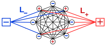
Figure 1: The complete-graph system. Two opposing news sources (squares) influence voters (circles) on the complete graph. The news sources have $L_{+}$ and $L_{-}$ links to individual voters.

The opinion evolution depends on the actual connection pattern between the news sources and voters, a situation that is analytically intractable. This leads us to apply a simplification that we term the annealed-link approximation. Here, we replace the true transition rates for each voter on a given fixed-link realization by the average transition rate, in which a link to a news source occurs with probability proportional to the appropriate link density. We now apply this approximation to determine the three basic characteristics of the collective opinions, namely, $E_{+}(y)$, $T_{\rm con}(y)$, and $T_{\rm pol}(y)$. We first first need the transition rates $r^{+}(x)$ and $r^{-}(x)$ within the annealed-link approximation. By a somewhat tedious but straightforward calculation (see A.2 for details), these rates are

$$\begin{split}r^{+}(x)&=\tfrac{1}{2}ANx(1-x)+B_{+}(1-x)\,,\\ r^{-}(x)&=\tfrac{1}{2}ANx(1-x)+B_{-}x\,.\end{split}$$ (9)

The $A$ terms account for the rate at which voters adopt the opinion of neighboring voters, while the $B$ terms account for opinion changes due to the interaction of voters with news sources. As shown in A.2, the amplitudes $A$ and $B_{\pm}$ are

$$A= \frac{(1\!-\!\ell_{+})(1\!-\!\ell_{-})}{1\!-\!(1/N)}+\frac{(1-p)(\ell_{+}+\ell_{-}-2\ell_{+}\ell_{-})}{(1-p)+(2p-1)/N}+\frac{(1-p)\ell_{+}\ell_{-}}{(1-p)+(3p-1)/N}\,,$$ (10a)

$$B_{\pm} =\frac{p\ell_{\pm}}{2}\!\left[\frac{1\!-\!\ell_{\mp}}{(1\!-\!p)\!+\!(2p\!-\!1)/N}\!+\!\frac{\ell_{\mp}}{(1\!-\!p)\!+\!(3p\!-\!1)/N}\right]\,.$$ (10b)

The three distinct terms in $$A B_{\pm} A B_{\pm} N$$ account for voters that are not connected to any news source, connected to one news source, and connected to both news sources. Similarly, the two terms for account for voters that are connected to one news source or to both news sources, respectively. While the coefficients and are complicated, they greatly simplify in the large- limit, where

$$A\to 1\qquad B_{\pm}\to\frac{1}{2}\frac{p\ell_{\pm}}{(1-p)}~{}.$$ (10c)

Substituting the transition rates (9) in Eq. (2), the drift velocity and the diffusion coefficient are:

$$V(x)=\frac{B_{+}(1-x)-B_{-}x}{N}\,,\qquad D(x)=A\,\,\frac{x(1-x)}{2N}+\frac{B_{+}(1-x)+B_{-}x}{2N^{2}}~{}.$$ (11)

Using these quantities in the formalism of Sec. 2, we can compute the exit probability, the consensus time, and the polarization time for different link densities $\ell_{\pm}$. As a preliminary, we first study the influence of a single $+$ news source on voter opinions and then turn to the influence of two opposing news sources.

3.1 Single news source

When there is only a single news source, the opinion state of the population is monotonically driven to consensus that is aligned with the news source. We now determine its effectiveness in driving this consensus.

For a single news source, we set $\ell_{-}=0$ and $\ell_{+}=\ell$ in Eq. (11), from which

$$\frac{V(x)}{D(x)}=\frac{\alpha}{x+\alpha/(2N)}~{},$$ (12)

where $\alpha\equiv{2B_{+}}/{A}$, which approaches ${p\ell}/(1-p)$ as $N\to\infty$. The parameter $\alpha$ is fundamental, as it characterizes the effectiveness of the news source in influencing the population, both by its intrinsic persuasiveness and by the extent of its reach.

Using Eq. (12) in (3), the effective potential in which $x$ diffuses is

$$\phi(x)=-\alpha\ln\left(x+\frac{\alpha}{2N}\right)\,.$$ (13)

This asymmetric potential biases individual opinions towards the $+$ consensus state. We determine the exit probability by substituting the effective potential (13) into (5) and performing the integral to give

$$E_{+}(y)=\begin{cases}{\displaystyle\frac{\left(\alpha+2Ny\right)^{1-\alpha}-\alpha^{1-\alpha}}{\left(\alpha+2N\right)^{1-\alpha}-\alpha^{1-\alpha}}}\qquad&\alpha\neq 1\,,\\[12.80373pt] {\displaystyle\frac{\ln\left(2Ny+1\right)}{\ln\left(2N+1\right)}}\qquad&\alpha=1\,.\end{cases}$$ (14)

By increasing $\alpha$, the news source becomes more effective in biasing the opinions towards $+$ consensus, as shown in Fig. 2. Here, we choose $(p,\ell)=(\frac{1}{2},1)$ to achieve $\alpha=1$, and $(p,\ell)=(\frac{2}{3},1)$ to achieve $\alpha=2$. Unless otherwise stated, we use these parameter choices to generate systems with $\alpha=1$ and $\alpha=2$ in subsequent figures. The qualitative behavior in Fig. 2 is the same as exit probability of a biased random walk on a finite interval with bias to the right [45]. As expected, when the news source is very effective, the exit probability is nearly 1, even for $y$ close to 0.

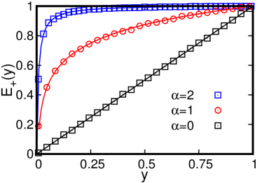
Figure 2: Exit probability versus initial fraction of $+$ opinion voters $y$ for $N=128$ voters that are influenced by single news source with link density $\ell=1$. The curves represent Eq. (14) and the symbols represent simulations over $10^{4}$ realizations.

To compute the consensus time, first note, from Eq. (12), that $V/D$ is of order 1, except when $x$ is of order $1/N$ or smaller. Within this boundary layer near $x=0$, the second term in the denominator of $V/D$ ensures that $V/D$ remains finite even when $x=0$. We can simplify the algebra considerably by excluding this thin boundary layer and correspondingly dropping this second term in the denominator of $V/D$. We checked numerically that this approximation has a vanishingly small effect on the consensus time for large $N$. We determine the range of the resulting slightly truncated interval $[a,1]$ by equating the two terms in the denominator of $V/D$ to give $a=\alpha/(2N)$. In this truncated interval, we have

$$V(x)=\frac{B_{+}(1\!-\!x)}{N}\qquad\qquad D(x)\approx\frac{Ax(1\!-\!x)}{2N}\,.$$ (15)

With these simplifications, the effective potential becomes $\phi(x)=-\alpha\ln x$ for $x\in[a,1]$.

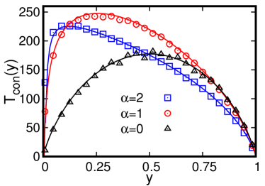
Figure 3: Consensus time versus the initial fraction of $+$ opinion voters $y$ for $N=128$ voters with a single news source. The solid curves represent Eq. (16) and the symbols represent simulation results over $10^{4}$ realizations.

We now substitute this effective potential, as well as the above form for $D(x)$, into the first of Eqs. (7). The resulting integral can be evaluated for certain simple values of $\alpha$. For the cases $\alpha=1$ and $\alpha=2$, in particular, we obtain

$$T_{\rm con}(y)=\begin{cases}{\displaystyle 2N\!\!\left[\frac{\ln(a/y)}{\ln a}\frac{\pi^{2}}{6}+\frac{\ln y}{\ln a}\,\,{\rm Li}_{2}(a)-{\rm Li}_{2}(y)\right]}&\qquad\alpha=1\,,\\[15.649pt] {\displaystyle 2N\Big{(}1-\frac{1}{y}\Big{)}\ln\frac{(1-y)}{(1-a)}}&\qquad\alpha=2\,,\end{cases}$$ (16)

where ${\rm Li}_{2}(y)$ is the dilogarithm function [46]. It is possible that analytical solutions also exist for other simple values of $\alpha$, but the results given above mostly encompass the generic behavior for a single news source; namely, the consensus time scales linearly with $N$, except in the limit $\alpha\to\infty$. When the initial state is $y=\frac{1}{2}$, we have

$$T_{\rm con}=\begin{cases}2N\ln 2\approx 1.386N&\qquad\alpha=0\\ \left(\ln^{2}2+\pi^{2}/6\right)N\approx 2.125N&\qquad\alpha=1\\ 2N\ln 2\approx 1.386N&\qquad\alpha=2\,.\end{cases}$$

The first line is the complete-graph VM result without news sources. Because the news source biases the population to $+$ consensus, the maximum of $T_{\rm con}(y)$ shifts gradually towards $x=0$, as shown in Fig. 3. Coincidentally, the consensus time starting from $y=\frac{1}{2}$ is the same for $\alpha=0$ and $\alpha=2$.

In the opposite limit of $\alpha\to\infty$, the consensus time scales as $\ln N$. This limit is conveniently realized by choosing $\ell=1$ and $p\to 1$. Then Eq. (10) gives $A\approx\frac{1}{2}N(1-p)$ and $B_{+}\approx\frac{1}{2}N$, so that $\alpha={2B_{+}}/{A}\approx 2/(1-p)$. When $1-p\ll\frac{2}{N}$, $A$ is vanishingly small, so the forward rate $r^{+}(x)\approx B_{+}(1-x)$ and the backward rate $r^{-}(x)\approx 0$. Thus the fraction of $+$ voters only increases with time until $+$ consensus is reached. For the initial condition $x=\frac{1}{2}$, we determine the consensus time from

$$T_{\rm con}=\sum^{1-\frac{1}{N}}_{x=\frac{1}{2}}\frac{1}{r^{+}(x)}=\sum^{1-\frac{1}{N}}_{x=\frac{1}{2}}\frac{1}{B_{+}(1-x)}\simeq 2\ln N\,.$$

3.2 Two opposing news sources

We now turn to our main focus of two opposing news sources. To determine the exit probability, as well as the consensus and polarization times, we again need to simplify the form of the drift velocity and the diffusion coefficient in Eq. (11). Again, the ratio $V/D$ is of order 1, except when $x$ is a distance of order $1/N$ from the boundaries at 0 and 1. The algebra simplifies considerably when we ignore these boundary layers. Following the same procedure as in the previous subsection, the second term in the denominator of $V/D$ can be neglected when $x$ is in the range $[a_{-},1-a_{+}]$, with $a_{\pm}={B_{\mp}}/{AN}$. In this truncated interval, we may write

$$V(x)=\frac{\left[B_{+}(1\!-\!x)-B_{-}x\right]}{N}\qquad\qquad D(x)\approx\frac{Ax(1\!-\!x)}{2N}\,.$$ (17)

Using this approximation for $V(x)$ and $D(x)$, the effective potential (3) becomes

$$\phi(x)=-\ln[x^{\alpha_{+}}(1-x)^{\alpha_{-}}]\,,$$ (18)

with $\alpha_{\pm}=2B_{\pm}/A\approx p\ell_{\pm}/(1-p)$. Thus in the presence of opposing news sources, the density $x$ undergoes diffusive dynamics in the (generally) asymmetric logarithmic potential well (18). Because of this well, the consensus time can be much longer than in the case of no news sources, as we would naively expect. However, because the potential at the interval boundaries depends logarithmically on $N$, the consensus time grows only algebraically, rather than exponentially, with $N$.

3.2.1 Symmetrically connected news sources

For simplicity, first consider equally connected news sources and define the common link density as $\ell\equiv\ell_{\pm}$. Now the parameter that quantifies the effectiveness of the news sources is $\alpha=\alpha_{\pm}\approx p\ell/(1-p)$, while the effective potential simplifies to $\phi(x)=-\alpha\ln\left[x(1-x)\right]$. Moreover, the relevant range of $x$ is $a\leq x\leq 1-a$, where $a_{+}=a_{-}\equiv a=\alpha/(2N)$.

To obtain the exit probability, we substitute the symmetrized version of Eq. (17) into Eq. (5) and evaluate the integral to obtain

$$E_{+}(y)=\frac{1}{2}\bigg{[}1-\frac{G_{\alpha}(y)}{G_{\alpha}(a)}\bigg{]}\,,$$ (19)

where, for simple rational values of $\alpha$, $G_{\alpha}$ can be determined analytically. The specific examples that we could compute are:

$$G_{\frac{1}{2}}(y) =\sin^{-1}\!\sqrt{y}-\frac{\pi}{4}$$

$$G_{1}(y) =\ln\left(y^{-1}-1\right)$$

$$G_{\frac{3}{2}}(y) =\sqrt{y(1-y)^{-1}}-\sqrt{y^{-1}(1-y)}$$

$$G_{2}(y) =y^{-1}-(1-y)^{-1}+\ln\left(y^{-1}-1\right)^{2}\,.$$

By plotting these expressions, we find that the exit probability has an anti-sigmoidal shape for $\alpha>0$ (Fig. 4). This behavior reflects the opposing role of the two news sources. If the initial density of the system is $y\neq\frac{1}{2}$, the news sources tend to drive the opinions to the politically polarized state of $y=\frac{1}{2}$ before consensus is reached. Consequently, the exit probability becomes nearly independent of the initial condition as the news sources become more effective, i.e., $\alpha\gg 1$.

Figure 4: Exit probability to $+$ consensus versus $y$ for $N=128$ voters with opposing and symmetrically linked news sources. Equation (19) gives the curves and the symbols correspond to simulations over $10^{4}$ realizations.

For the consensus time, we again substitute the symmetrized form of Eq. (17) into the first of Eqs. (7) and evaluate the integral to give

$$T_{\rm con}(y)=N\left[H_{\alpha}(a)-H_{\alpha}(y)\right]$$ (20)

where, once again, $H_{\alpha}$ can be determined explicitly for certain rational values of $\alpha$:

$$H_{\frac{1}{2}}(y) =-4\sin^{-1}\!\!\sqrt{y}\,\,\,\sin^{-1}\!\!\sqrt{1-y}\,,$$

$$H_{1}(y) =-\ln\left[y(1-y)\right]\,,$$

$$H_{\frac{3}{2}}(y) =\frac{(2y-1)}{\sqrt{4y(1-y)}}\left[\sin^{-1}\!\!\sqrt{y}-\sin^{-1}\!\!\sqrt{1-y}\right]\,,$$

$$H_{2}(y) =\tfrac{1}{6}\left[y^{-1}(1-y)^{-1}-2\ln\left[y(1-y)\right]\right]\,.$$

We can determine the $N$ dependence of the consensus time from the large-$N$ behavior of the functions $H_{\alpha}(a)$ with $a=\alpha/(2N)$. The dominant contribution for large $N$ arises from the term $H_{\alpha}(a)$ with $a\to 0$:

$$H_{\frac{1}{2}}(a) \sim a^{1/2}$$

$$H_{1}(a) \sim-\ln a$$

$$H_{\frac{3}{2}}(a) \sim a^{-1/2}$$

$$H_{2}(a) \sim a^{-1}\,.$$

Using $a=\alpha/2N$ and combining the above results with Eq. (20), we find

$$T_{\rm con}\sim\begin{cases}N&\qquad 0\leq\alpha<1\,,\\ N\ln N&\qquad\alpha=1\,,\\ N^{\alpha}&\qquad\alpha>1\,.\end{cases}$$ (21)

Equation (21) is one of our major results.

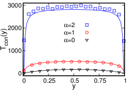
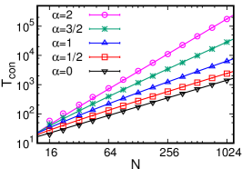
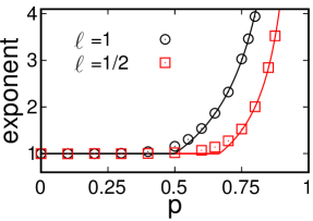
Figure 5: (a) Consensus time versus $y$. Equation (20) gives the curves and symbols represent simulations results for $N=128$ voters over $10^{4}$ realizations. (b) Consensus time versus $N$. The curves again represent the predictions from Eq. (20). We fix $\ell=1$ and use $\alpha=p/(1-p)$ to specify $p$ for a given $\alpha$ value. (c) Consensus time exponent versus $p$ for two $\ell$ values. The symbols represent simulation results and the curves are predictions from Eq. (21).

Our simulation results are consistent with these predictions (Fig. 5). A striking feature of Fig. 5(a) is that the consensus time increases dramatically when $\alpha$ increases from 1 to 2. This behavior reflects the different $N$ dependences of the consensus time for $\alpha<1$ and $\alpha\geq 1$ in Eq. (21). Our estimates for the consensus time exponent for various combinations of $p$ and $\ell$ are given in Fig. 5(c). We determine the exponent by extrapolating local slopes of $\ln T_{\rm con}$ versus $\ln N$ based least-squares fits of subsets of successive data points. For each $p$ and $\ell$, $\alpha$ is given by $\alpha=p\ell/(1-p)$. The sudden increase in the exponent value at the two distinct $p$ values corresponds to the transition at $\alpha=1$ predicted by (21).

There are two natural ways that the news sources are connected to voters: (i) random connections, and (ii) disjoint connections. In the first case, a voter may be connected to zero, one, or two news sources, while in the latter, a voter may be connected to either zero or one news source. For the same link densities between the news sources and voters, we found negligible differences in our results for the exit probability and the consensus and polarization times. The simulation results presented here are for the case of random connections.

We can understand the $N$ and $\alpha$ dependences of the consensus time in a simple way in terms of the effective potential (18). According Kramers’ theory [48], the time to reach the boundaries at $a$ and at $1-a$ are proportional to $\exp[\phi(a)]$ and to $\exp[\phi(1-a)]$, respectively, while the potential at these two points scales as $\alpha\ln N$. Consequently $T_{\rm con}\sim N^{\alpha}$ for $\alpha>1$. For $\alpha<1$, the effect of the logarithmic potential is subdominant with respect to fluctuations [49], and it is the latter drive the system to consensus, leading to $T_{\rm con}\sim N$.

We now determine the polarization time. Substituting the symmetric forms of the drift and diffusion coefficients from Eq. (17) into the second of Eq. (7) and evaluating the integral, which can be done for certain simple values of $\alpha$, we obtain:

$$T_{\rm pol}(y)=\begin{cases}4N\left(\frac{\pi}{4}-\sin^{-1}\!\sqrt{y}\right)\left(\frac{\pi}{4}+\sin^{-1}\!\sqrt{y}-2\sin^{-1}\!\sqrt{a}\right)~{}&\quad\alpha=\frac{1}{2}\,,\\[11.38109pt] 2N\left[a\ln y+(1-a)\ln(1-y)+\ln 2\right]~{}&\quad\alpha=1\,,\\[11.38109pt] \frac{N(2y-1)}{\sqrt{y(1-y)}}\left[\sin^{-1}\!\sqrt{a}-\sin^{-1}\!\sqrt{y}-(1\!-\!2a)\sqrt{a(1\!-\!a)}\right]~{}&\quad\alpha=\frac{3}{2}\,,\\[11.38109pt] \tfrac{1}{3}N\left\{2+2\ln[2(1\!-\!y)]-\frac{1}{1-y}-a^{2}(3\!-\!2a)\left[\frac{1-2y}{y(1-y)}+2\ln\frac{(1-y)}{y}\right]\right\}~{}&\quad\alpha=2\,.\end{cases}$$ (22)

The main qualitative feature of $T_{\rm pol}(y)$ is that it is maximal for $y\to 0$ and decreases to 0 as $y\to\frac{1}{2}$. The $N$ dependence of the maximal polarization time may be found by setting $y=a=\alpha/(2N)$ in Eq. (22) and keeping the dominant contribution. This gives:

$$T_{\rm pol}\simeq\begin{cases}\frac{1}{4}\pi^{2}N\approx 2.467N&\quad\alpha=\frac{1}{2}\,,\\[2.84526pt] 2\ln 2N\approx 1.386N&\quad\alpha=1\,,\\[2.84526pt] N&\quad\alpha=\frac{3}{2}\,,\\[2.84526pt] \frac{1}{3}(1+2\ln 2)N\approx 0.795N&\quad\alpha=2;\end{cases}$$

that is, the maximal value of the polarization time scales linearly with $N$.

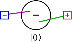
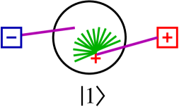
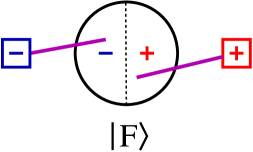
Figure 6: The three states in the reduced state space of the complete-graph system with a single link from each news source: (a) the initial consensus state $|0\rangle$. Active and inactive links are shown in green and magenta. (b) The excited state $|1\rangle$, where the single voter linked to the $+$ news source changes its opinion to $+$ and now disagrees with all its $N-1$ neighbors, leading to many active links. (c) The final polarized state $|F\rangle$; here the active links are not shown.

However, the polarization time grows faster than linearly in $N$ for sufficiently small $\alpha$, corresponding to weak news sources. To understand the behavior in this limit, it is instructive to consider the extreme limit where each news source is connected to a single voter (Fig. 6). Suppose that the population starts in the $-$ consensus state. At some point, an “informed” voter (the one linked to the $+$ news source) changes its opinion from $-$ to $+$ by interacting with the news source. When this happens, this informed voter now disagrees with all its neighbors. From this excited state, subsequent opinion changes are primarily caused by disagreeing voters within the complete graph because links between voters are numerous and there is only one link to the news source. Thus the voters undergo classic VM dynamics, as long as there is any disagreement.

Within this picture, we can reduce the dynamics to a three-state space (Fig. 7): the state $|0\rangle$, corresponding to $-$ consensus ($x=0$), in which only the news source influences the voters, the final polarized state $|F\rangle$ ($x=\frac{1}{2}$), and the excited state $|1\rangle$, in which one voter in the complete graph has the $+$ opinion. As indicated in Fig. 6(b), the news source has a negligible influence on this excited state. After this reduction, it is straightforward to compute the time to reach the polarized state $|F\rangle$ starting from the initial consensus state $|0\rangle$ by applying first-passage ideas [45]. Starting from $|0\rangle$, the state $|1\rangle$ is necessarily reached, so the transition probability from $|0\rangle$ to $|1\rangle$ equals 1. Similarly, $E=\frac{2}{N}$ is the probability to reach polarized state $|F\rangle$ from $|1\rangle$ by VM dynamics (that is, one $+$ voter initially and $\frac{N}{2}$ $+$ voters in the final state). This portion of the dynamics coincide with the VM because the news sources play no role.

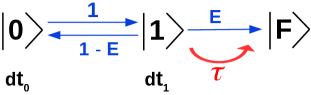
Figure 7: The transition rates and transition times in the reduced system.

We define $T_{0}$ and $T_{1}$ as the first-passage times to reach the polarized state from the initial states $|0\rangle$ and $|1\rangle$ respectively. These first-passage times satisfy

$$\begin{split}T_{0}&=dt_{0}+T_{0}^{\prime}\,,\\ T_{1}&=E\tau\ +(1\!-\!E)(dt_{1}+T_{1})\,,\end{split}$$ (23)

where, from Eq. (9),

$$dt_{0} =1/[r^{+}(0)\!+\!r^{-}(0)]=2/\alpha\,,$$

$$dt_{1} =1/\big{[}r^{+}(\tfrac{1}{N})\!+\!r^{-}(\tfrac{1}{N})\big{]}\approx 1\,,$$

are the transition times to leave the states $|0\rangle$ and $|1\rangle$, respectively, and $\tau=2N(1-\ln 2)$ is the conditional time to reach the final state $|F\rangle$ from $|1\rangle$ by VM dynamics (B). Solving Eqs. (23) gives,

$$T_{\rm pol} \equiv T_{0}=\tau+\frac{dt_{0}}{E}+\frac{(1-E)dt_{1}}{E}\approx N\left(\tfrac{5}{2}-2\ln 2\right)+\frac{N}{\alpha}.$$ (24)

Thus the polarization time scales linearly with $N$, unless $\alpha\to 0$. This limit of $\alpha\to 0$ is achieved, for example, when a single link connects the news source to voters. In this case, $\alpha=p\ell/(1-p)=p/[N(1-p)]$, which gives $T_{\rm pol}\sim N^{2}(1-p)/p$.

3.2.2 Asymmetrically connected news sources

When the number of links from the two news sources differ, the density $x$ now diffuses in an asymmetric logarithmic potential. To achieve consensus, $x$ has to surmount one of the potential barriers, either at $a_{-}$ or at $1-a_{+}$, with respective barrier heights $\alpha_{+}\ln N$ and $\alpha_{-}\ln N$. Again from Kramers’ theory, the dominant contribution to the consensus time scales exponentially in the lowest barrier height, as long as the barrier height grows at least as fast as $\ln N$. Thus the consensus time scales as $N^{\alpha}$, with consensus time exponent now given by $\alpha=\min(\alpha_{+},\alpha_{-},1)$. To test this hypothesis, we show the $N$ dependence of $T_{\rm con}$ from simulations in Fig. 8 for two combinations of unequal link densities. For $(\alpha_{+},\alpha_{-})=(\frac{3}{2},\frac{1}{2})$, the consensus time scales linearly with $N$, while for $(\alpha_{+},\alpha_{-})=(\frac{3}{2},2)$, the consensus time scales as $N^{3/2}$, as we expect. In the simulations, we fix $p=\frac{2}{3}$ and $\ell_{+}=\frac{3}{4}$ to give $\alpha_{+}=\frac{3}{2}$, and then use $\ell_{-}=\frac{1}{4}$ to give $\alpha_{-}=\frac{1}{2}$ and $\ell_{-}=1$ to give $\alpha_{-}=2$.

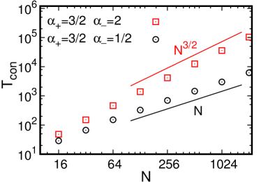
Figure 8: The consensus time versus $N$ for voters influenced by two news sources with unequal link densities. The data are from simulations over $10^{4}$ realizations. The lines are guides for the eye.

Another basic characteristic of the collective opinion state is its distribution. The opposing nature of the two news sources drives the population to a steady state in the long-time limit. We obtain the steady-state opinion distribution, $P_{\rm ss}(x)\equiv P(x,t\rightarrow\infty)$, by setting ${\partial P}/{\partial t}=0$ in the Fokker-Planck equation (1b) and then solving. To have a well-posed problem, we need to specify the boundary conditions. The appropriate conditions are reflection at $x=a_{-}$ and $x=1-a_{+}$ because for all $\alpha>0$, the endpoints are not fixed points of the stochastic dynamics. Solving this Fokker-Planck equation and imposing normalization, $\int^{1-a_{+}}_{a_{-}}P_{\rm ss}(x)dx=1$, we obtain

$$P_{\rm ss}(x)=\frac{x^{\alpha_{+}-1}(1-x)^{\alpha_{-}-1}}{{B}\left[1-a_{+};\alpha_{+},\alpha_{-}\right]-{B}\left[a_{-};\alpha_{+},\alpha_{-}\right]}\,,$$ (25)

where $B(x;y,z)$ is the incomplete beta function [46].

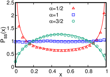
Figure 9: Steady-state distribution of $x$ for 128 voters. The curves are the predictions of Eq. (25) and symbols represent simulations.

In the symmetric case, $\ell_{\pm}=\ell$, this distribution reduces to $P_{\rm ss}(x)\propto[x(1-x)]^{\alpha-1}$, which undergoes a bimodal to unimodal transition as $\alpha$ passes through 1 (Fig. 9). In this figure, we fix $\ell=1$ and use $\alpha=p\ell/(1-p)$ with appropriate values of $p$ to give $\alpha=\frac{1}{2},1$, and $\frac{3}{2}$, and then evolve the system until the steady state is reached (typically for times greater than $10^{6}$). When $\alpha<1$, the distribution has maxima at $x=0,1$. That is, for weak news sources, the population typically remains close to one of the two consensus states. Conversely, for influential news sources ($\alpha>1$) the steady-state distribution has a maximum at $x=1/2$, corresponding to the politically polarized state. In the marginal case of $\alpha=1$, all possible opinion states are equally likely.

4 Voters on a two-clique graph

We now investigate the influence of two opposing news sources when the voters reside on a two-clique graph, with $N$ voters in each clique (Fig. 10). The $+$ news source connects to random voters on $C_{+}$ via $L_{+}$ links and the $-$ news source connects to random voters on $C_{-}$ via $L_{-}$ links. We write $\ell_{\pm}=L_{\pm}/N$ as the corresponding link densities. To simplify matters, we restrict ourselves to the case of equally connected news sources, $\ell_{+}=\ell_{-}\equiv\ell$. However, the voter model on the two-clique graph with unequal-size cliques was very recently investigated in [47], where a non-monotonic dependence of the consensus time on interclique density was found. In our symmetric two-clique graph, the voters on different cliques are connected by $L_{0}=N^{\beta}$ interclique links, with $0\leq\beta\leq 2$. For $L_{0}\to N^{2}$, the two cliques together form a complete graph of $2N$ voters. We focus on the interesting (and realistic) case where the cliques are sparsely interconnected ($\beta\to 0$).

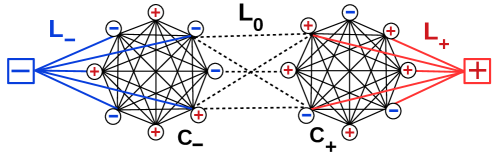
Figure 10: The two-clique system, with two opposing news sources (squares) and voters (circles). Each clique contains $N$ voters, with $L_{0}$ links between cliques $C_{+}$ and $C_{-}$.

Let $x_{1}$ and $x_{2}$ denote the fraction of $+$ opinion voters on clique $C_{+}$ and $C_{-}$, respectively, at time $t$. We represent the state of the system by the clique densities $(x_{1},x_{2})$. Let $r_{i}^{\pm}(x_{1},x_{2})$ be the rates for $x_{i}$ to change by $\pm\delta x$. Within the annealed-link approximation, these rates are (see A.3 for details):

$$r_{1}^{+}(x_{1},x_{2}) =\tfrac{1}{2}A\left[Nx_{1}(1\!-\!x_{1})+\ell_{0}(1\!-\!x_{1})x_{2}\right]+B(1\!-\!x_{1})$$

$$r_{1}^{-}(x_{1},x_{2}) =\tfrac{1}{2}A\left[Nx_{1}(1\!-\!x_{1})+\ell_{0}\,x_{1}(1\!-\!x_{2})\right]$$

$$r_{2}^{+}(x_{1},x_{2}) =\tfrac{1}{2}A\left[Nx_{2}(1\!-\!x_{2})+\ell_{0}\,x_{1}(1\!-\!x_{2})\right]$$

$$r_{2}^{-}(x_{1},x_{2}) =\tfrac{1}{2}A\left[Nx_{2}(1\!-\!x_{2})+\ell_{0}(1\!-\!x_{1})x_{2}\right]+Bx_{2}$$ (26)

where $\ell_{0}=L_{0}/N=N^{\beta-1}$ is the number of voters in $C_{+}$ that link to a voter in $C_{-}$ or vice versa, and the coefficients $A$ and $B$ are

$$\begin{split}A&=\frac{\ell(1-p)N}{(1-p)(N+\ell_{0}-1)+p}+\frac{(1-\ell)N}{N+\ell_{0}-1}~{},\\[5.69054pt] B&=\frac{\ell pN}{2[(1-p)(N+\ell_{0}-1)+p]}~{}.\end{split}$$ (27a)

Ignoring terms of order $$1/N$$, these coefficients reduce to

$$A\approx\frac{N}{N+\ell_{0}}\,,\qquad B\approx\frac{\ell p}{2(1-p)}\,.$$ (27b)

Let $P(x_{1},x_{2})\,\delta x^{2}$ be the probability for the opinion state of the population to be within a range $\delta x^{2}$ about $(x_{1},x_{2})$. Expanding the underlying master equation in a Taylor series to second order gives the two-variable Fokker-Planck equation

$$\frac{\partial}{\partial t}P(x_{1},x_{2},t)=\sum^{2}_{i=1}\left\{-\frac{\partial}{\partial x_{i}}[V_{i}P]+\frac{\partial^{2}}{\partial x_{i}^{2}}[D_{i}P]\right\}\,,$$ (28)

where

$$V_{i}(x_{1},x_{2}) =[r_{i}^{+}(x_{1},x_{2})-r_{i}^{-}(x_{1},x_{2})]\delta x\,,$$

$$D_{i}(x_{1},x_{2}) =[r_{i}^{+}(x_{1},x_{2})+r_{i}^{-}(x_{1},x_{2})](\delta x^{2}/2)\,.$$

The coupling between $x_{1}$ and $x_{2}$ arises because a change in $x_{1}$ alters $V_{2}$ and $D_{2}$, and vice versa for $x_{2}$. Because of this complication, an analytical approach of the full dynamics appears to be challenging. However, Ref. [47] has made progress in this direction.

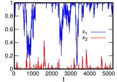
Figure 11: (a) Typical trajectories for $x_{1}$ and $x_{2}$ in the two-clique graph with $N=128$, $\beta=0.5$, and $\alpha=2$ ($\ell=1$ and $p=2/3$). (b) Distribution of fraction $x_{1}$ of $+$ opinion voters on clique $C_{+}$ of 128 voters on the two-clique graph, with $\ell=1$.

To make progress, it is helpful to first study the time evolution of the trajectories of $x_{1}$ and $x_{2}$ for sparsely connected cliques (Fig. 11(a)). The population spends a large fraction of the time in the neighborhood of the state $(x_{1}\!=\!1,x_{2}\!=\!0)$, which we term the maximally polarized (MP) state. The population tends to remain close to the MP state because: (i) the news sources tend to drive the clique opinions to this state, and (ii) the transition time to leave the MP state,

$$dt_{0}=\left[r_{1}^{+}(1,0)+r_{1}^{-}(1,0)+r_{2}^{+}(1,0)+r_{2}^{-}(1,0)\right]^{-1}\,,$$

scales as $N^{1-\beta}$, which becomes large as $\beta\to 0$. These two properties is reflected in the steady-state opinion distribution in each clique (Fig. 11(b)). As shown in the figure, this distribution becomes more concentrated near $x_{1}=1$ as either the number of interclique links is reduced or the interactions with news sources become stronger. (By symmetry, the opinion distribution on $C_{-}$ is concentrated near $x_{2}=0$.)

    

    

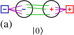
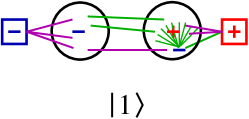
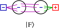
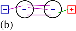
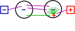
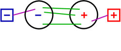
Figure 12: (a) The reduced states to determine the consensus time for the two-clique graph: (left) the initial maximally polarized state $|0\rangle$. (middle) The excited state $|1\rangle$, in which one voter in clique $C+$ has changed opinion from $+$ to $-$. (right) The final consensus state $|F\rangle$. (b) Reduced states of the two-clique graph to determine the polarization time: (left) the initial consensus state $|0\rangle$. (middle) The excited state $|1\rangle$, in which one voter in clique $C+$ has changed opinion from $-$ to $+$. (right) The final maximally polarized state $|F\rangle$.

In the limit of sparsely connected cliques, we may again reduce the state space (Fig. 12(a)), analogous to the construction given in Figs. 6 and 7, to determine the consensus time for the complete-graph system. First, note that the $N^{\beta}$ interclique links are relevant only in the MP state. In all other opinion states, the dynamics is controlled by the $\frac{1}{2}N(N-1)\gg N^{\beta}$ intraclique links. Thus we can view the system as being comprised of two isolated cliques, with one clique inactive (where all voters agree with the news source) and the other clique, where the voters are not in consensus, active.

Starting in the MP state, suppose that one voter in $C_{+}$ changes opinion from $+$ to $-$ due to an interaction with a $-$ voter in $C_{-}$. The population is now in the excited state $\big{(}1-\frac{1}{N},0\big{)}$ where the $-$ voter in $C_{+}$ differs with the rest of its $N-1$ neighbors. Because interclique links are sparse $(\beta\to 0)$ and the number of intraclique links between voters with differing opinions in $C_{+}$ is of order $N$, the opinion dynamics is driven by the latter class of links. For the active clique $C_{+}$, there are two possible outcomes starting from the excited state $\big{(}1-\frac{1}{N},0\big{)}$. Either $C_{+}$ returns to $+$ consensus (and the full system returns to the MP state) or $C_{+}$ reaches $-$ consensus. We again visualize the MP state $(1,0)$ as $|0\rangle$, the excited state $\big{(}1-\frac{1}{N},0\big{)}$ as $|1\rangle$, and the $-$ consensus state $(0,0)$ as the final state $|F\rangle$ (Fig. 12(a)). With these reduced states, we obtain the consensus time by the same calculation as that given in the previous subsection to determine the polarization time for the complete graph.

Starting from the state $|0\rangle$, the system moves to state $|1\rangle$ after a transition time $dt_{0}=N^{1-\beta}$. The time to reach the final consensus state starting from $|0\rangle$ satisfies

$$T_{0}=dt_{0}+T_{1}\,.$$ (29a)

where $$T_{1} |1\rangle |1\rangle (x_{1},x_{2})=\big{(}1-\frac{1}{N},0\big{)} |1\rangle dt_{1}\approx(1+\ell_{0})^{-1} |1\rangle |2\rangle E=1-E_{+}\big{(}1\!-\!\frac{1}{N}\big{)} E_{+}(y) |2\rangle |1\rangle \tau T_{1}$$ is the time to reach consensus from the initial state . Substituting the state densities into the rates (4), the transition time to leave state is . Starting from , the probability for the active clique to reach the state is , with given in Eq. (14). We also define the mean conditional time to reach from as . Then satisfies

$$T_{1}=E\tau+(1-E)(dt_{1}+T_{0})\,.$$ (29b)

Solving these equations gives

$$T_{0}\equiv T_{\rm con}=\tau+\frac{dt_{0}}{E}+\frac{(1-E)dt_{1}}{E}\,.$$ (30)

In the limit $\beta\to 0$, $\tau$ is subdominant (see C) and $dt_{1}\ll dt_{0}$, so that the third term is also subdominant. Thus keeping only the dominant term $dt_{0}/E$, the consensus time has scaling behavior:

$$T_{\rm con}\sim\begin{cases}N^{2-\beta}\quad&\alpha<1\,,\\ N^{2-\beta}\ln N\quad&\alpha=1\,,\\ N^{1+\alpha-\beta}\quad&\alpha>1\,.\end{cases}$$ (31)

The consensus time exponent increases as interclique links become more rare and also as the influence of news sources increases beyond $\alpha\geq 1$ (Fig. 13(a)). The data in this figure corresponds to fixed $\beta=\frac{1}{2}$ and $\ell=1$, and $p$ is varied to give the $\alpha$ values shown. Figure 13(b) shows the consensus time exponent as a function of $p$ for fixed $\ell$, as well as the comparison with our basic prediction Eq. (31). Our results for the consensus time are consistent with previous studies [47, 50] of the VM on the two-clique graph.

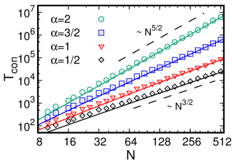
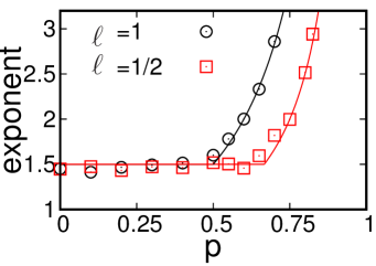
Figure 13: (a) Consensus time versus $N$ for voters on a two-clique graph. The solid lines give $dt_{0}/E$ from Eq. (30) and the symbols represent simulations over $10^{3}$ realizations. (b) Consensus time exponent as a function of $p$. The symbols are the simulation results and the curves are the predictions of Eq. (31).

For the polarization time, we again use a reduced state-space approach, analogous to that developed to derive Eq. (24) for the complete-graph system. For concreteness and simplicity, we start the system in the $-$ consensus state $(0,0)$ (Fig. 12(b)) and determine the time to reach the $(1,0)$ MP state in the interesting limit of weak news sources and weak intraclique connections. We now denote the $(0,0)$ consensus state as $|0\rangle$, the excited state $\big{(}\frac{1}{N},0\big{)}$, where a single voter in clique $C_{+}$ has changed opinion, as $|1\rangle$, and the MP state as $|F\rangle$, respectively (Fig. 7). In state $|0\rangle$, the opinion change that leads to state $|1\rangle$ is caused only by the link between a voter and the $+$ news source. In $|1\rangle$, subsequent opinion changes occur by classic VM dynamics because interclique links significantly outnumber all other links and the effect of the latter can be ignored.

Referring to Fig. 12(b), let $dt_{0}$ and $dt_{1}$ denote the transition times out of the states $|0\rangle$ and $|1\rangle$ respectively. These transition times are the inverse of the sum of the rates out of these states. To obtain $dt_{0}$ we substitute $(x_{1},x_{2})=(0,0)$ into the rates (4) and obtain, after straightforward steps, $dt_{0}=2(1-p)/p\ell$. Similarly for $dt_{1}$, we substitute $(x_{1},x_{2})=\big{(}\frac{1}{N},0\big{)}$ into (4) and ultimately obtain $dt_{1}\approx 1$ for large $N$ and $\ell\to 0$. Let $E$ denote the exit probability to reach $|F\rangle$ starting from $|1\rangle$ without reaching $|0\rangle$; thus $1-E$ is the probability to reach $|0\rangle$ without reaching $|F\rangle$. Because the opinions evolve according to the classic VM dynamics when the system is in state $|1\rangle$, $E=1-\frac{1}{N}$ and the conditional time to reach $|2\rangle$ from $|1\rangle$ is $\tau=2N$, (C). Let $T_{0}$ and $T_{1}$ be the first-passage times to $|F\rangle$ starting from the initial states $|0\rangle$ and $|1\rangle$. These first-passage times again satisfy Eqs. (23) whose solution now is

$$T_{\rm pol}=\tau+\frac{dt_{0}}{E}+\frac{(1-E)dt_{1}}{E}\approx 3N+\frac{2N}{\alpha}~{}.$$ (32)

The main message from this result is that as soon as the news sources connect to a non-vanishing fraction of the population, the polarization time is of order $N$, and is generally much smaller that the consensus time when $\alpha$ is large.

5 Summary

We introduced an opinion dynamics model where individuals that change their opinions by VM dynamics are also influenced by two fixed and opposing news sources. Our model is motivated by the current polarized political state in Europe and the US [51, 52, 53, 54, 55, 56, 57], as well as by the recent emergence of biased news sources that promulgate fixed political viewpoints [58, 59, 60]. Our interest was to investigate the consequences of political polarization, which seem to be largely influenced by these types of news sources. In the VM framework, the two news sources are zealots that never change their opinion, but which influence the opinions of individual voters. Voters, on the other hand, may consult either news sources or neighboring voters to update their opinion state. The strength of the news sources is quantified by a single parameter $\alpha$, which encapsulates their degree of connection to the population and the relative likelihood that a voter consults a news source rather than a fellow voter. We developed a general framework to understand the rich dynamics of this model.

Our modeling relies on using highly idealized social networks. The two examples that we studied were the complete graph of $N$ voters and, more realistically, the two-clique graph with $N$ voters in each clique. The primary reason for this extreme level of idealization is to formulate analytically tractable models. In the complete graph, the news sources connect either to disjoint or to random voters; both subcases gave virtually identical results. In the two-clique graph, each news source connects to voters in disjoint cliques. With this modeling perspective, we can understand many properties of the opinion dynamics analytically. The analytical approach also allows us to develop insights that would be extremely difficult to reach through numerical simulations of our model on realistic social networks.

We studied basic characteristics of the collective opinion state including: the exit probability, the consensus time, and the polarization time. Generally, the consensus time increases while the polarization time decreases as the news sources becomes more influential. This behavior can be understood in terms of a diffusion-like picture for the opinion evolution. For the complete graph, the fraction $x$ of $+$ voters can be viewed as an effective particle that undergoes convection-diffusion in the interval $[0,1]$ in the presence of an effective potential. Reaching consensus corresponds to the effective particle surmounting the potential barriers near $x=0$ or $x=1$, while reaching the polarized state corresponds to the effective particle being pushed to the minimum of the potential. This potential picture explains why the consensus time is much longer than the polarization time. This disparity was also reflected in the steady-state opinion distribution, which undergoes a transition from a bimodal to a unimodal state as the influences of news sources is increased.

The existence of an effective potential implies that the magnetization, namely, the difference in the fraction of $+$ and $-$ voters, is not conserved by the dynamics. In previous studies of variants of the VM with non-conserved magnetization, the consensus time was found to grow faster than any power law in $N$ (see, e.g., [28, 29, 31]). In constrast, in this work the effective potential at the boundaries scales logarithmically in $N$, which leads to a power-law dependence of the consensus time on $N$, with a non-universal exponent.

We also found that voters on a two-clique graph are driven to a maximally polarized state in which voters on two different cliques independently reach unanimity but in opposite opinion states. The driving mechanism towards this state becomes stronger either when the number of interclique links is reduced or when the influence of news sources is increased. Weakly interconnected societies are very common around us because of social segregation, geopolitics (e.g., countries, states, etc.), and cultural differences (language, religion, etc.). All of these factors contribute to political polarization, and our modeling seems to capture an essence of this phenomenology. It would be worthwhile to allow the network itself to evolve to mimic the feature that societies are currently tending to increased fractionation.

We thank Mirta Galesic for helpful discussions and also gratefully acknowledge NSF financial support from grant DMR-1608211.

Appendix A Transition rates

To determine the transition rates $r^{\pm}(x)$, we need: (a) the elemental time step $\delta t$ for a single update, and (b) the probabilities $q^{\pm}(x)$ for $x$ to change by $\pm\delta x$ in an update. In terms of these quantities, the rates $r^{\pm}(x)$ are

$$r^{+}(x)=\frac{q^{+}(x)}{\delta t}\,,\qquad r^{-}(x)=\frac{q^{-}(x)}{\delta t}\,.$$ (33)

The probability for $x$ to not change in an update is $1-[r^{+}(x)+r^{-}(x)]\delta t=1-q^{+}(x)-q^{-}(x)$.

A.1 Voter on a complete graph

We first determine the rates for the VM on a complete graph of $N$ voters, where the elemental time step is $\delta t=2/N$. To find the probabilities, $q^{\pm}(x)$, first consider $q^{+}(x)$. For $x$ to increase, a $-$ voter has to be selected that then adopts the opinion of a neighboring $+$ voter. The probability to pick a $-$ voter is $N^{-}/N=(N-N^{+})/N$, where $N^{+}=Nx$ is the number of $+$ voters. The selected $-$ voter has $N-1$ neighbors, of which $N^{+}$ have opinion $+$. The probability for the $-$ voter to pick a $+$ neighbor is $N^{+}/(N-1)$. Therefore the probability for $x$ to increase by $\delta x$ is,

$$q^{+}(x)=\frac{N-N^{+}}{N}\frac{N^{+}}{N-1}=\frac{x(1-x)}{1-1/N}=q^{-}(x)\,.$$ (34)

The last equality follows from the $+-$ symmetry of the VM.

Substituting $q^{\pm}(x)$ and $\delta t=2/N$ into Eq. (33), the rates $r^{\pm}(x)$ are

$$r^{\pm}(x)=\frac{Nx(1-x)}{2(1-1/N)}\approx\frac{Nx(1-x)}{2}\,,$$ (35)

as quoted in Eq. (8).

A.2 Voters on a complete graph influenced by two news sources

Now consider voters on a complete graph that are additionally influenced by two news sources (Sec. 3). The system consists of $N+2$ agents: $N$ voters and two news sources, so that the elemental time step is $\delta t=2/(N+2)$. We now determine the probability $q^{+}(x)$ for a voter to adopt the opinion of a neighboring $+$ voter. The probability to pick a $-$ voter out of $N+2$ individuals is, $(N-N^{+})/(N+2)$. The $-$ voter has $N-1$ neighboring voters, but this voter may or may not be connected to the news sources. To find the probability that the selected $-$ voter changes its opinion, we have to consider four possibilities:

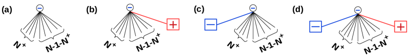
Figure 14: Possibilities for a $-$ voter (circle) to be connected to the news sources (squares). (a) The $-$ voter is connected to $N-1$ neighboring voters, with $N^{+}$ having $+$ opinion, but not to any news source. (b) The $-$ voter is connected to a $+$ news source, (c) connected to the $-$ news source, and (d) connected to both the news sources.

1. The $-$ voter is not connected to any news source [Fig. 14(a)]: the probability for this configuration is $(1-\ell_{+})(1-\ell_{-})$. The $-$ voter then adopts opinion from a neighboring $+$ voter with probability $N^{+}/(N-1)$. The contribution to $q^{+}(x)$ from this configuration is

   $$q_{1}=(1-\ell_{+})(1-\ell_{-})\frac{N^{+}}{N-1}\,.$$ (36a)

2. The $-$ voter is connected only to the $+$ news source (Fig. 14(b)), with probability $\ell_{+}(1-\ell_{-})$. The $-$ voter adopts the opinion of a neighboring $+$ voter with probability $(1-p)N^{+}/R$ or adopts the opinion of the $+$ news source with probability $p/R$, where $R=p+(N-1)(1-p)$. Thus the second contribution to $q^{+}(x)$

   $$q_{2}=\ell_{+}(1-\ell_{-})\frac{(1-p)N^{+}+p}{p+(N-1)(1-p)}\,.$$ (36b)

3. The $-$ voter is connected only to the $-$ news source (Fig. 14(c)), with probability $(1-\ell_{+})\ell_{-}$. The probability for the $-$ voter to adopt the opinion of a neighboring $+$ voter is $(1-p)N^{+}/R$, where $R=p+(N-1)(1-p)$. Thus the third contribution to $q^{+}(x)$ is,

   $$q_{3}=(1-\ell_{+})\ell_{-}\frac{(1-p)N^{+}}{p+(N-1)(1-p)}\,.$$ (36c)

4. The $-$ voter is connected to both the news sources (Fig. 14(d)) with probability $\ell_{+}\ell_{-}$. The $-$ voter thus adopts the opinion of a neighboring $+$ voter with probability $(1-p)N^{+}/R$ or adopts the opinion of the $+$ news source with probability $p/R$, where $R=2p+(N-1)(1-p)$. Thus the fourth contribution $q^{+}(x)$ is

   $$q_{4}=\ell_{+}\ell_{-}\frac{(1-p)N^{+}+p}{2p+(N-1)(1-p)}\,.$$ (36d)

We now write $q^{+}(x)=N^{-}(q_{1}+q_{2}+q_{3}+q_{4})/(N+2)$ and use $N^{-}=N-N^{+}$ , $N^{+}=Nx$, to obtain, after some rearrangement of terms

$$q^{+}(x)=\frac{1}{N+2}\left[ANx(1-x)+2B_{+}(1-x)\right]\,,$$ (37a)

where $$A B_{+} +-$$ and are defined in Eqs. (10). Using symmetry, we can also write

$$q^{-}(x)=\frac{1}{N+2}\left[ANx(1-x)+2B_{-}x\right]\,.$$ (37b)

In Eqs. (37), the first term inside the bracket accounts for voters that adopt the opinion of a neighboring voter and the second term accounts for voters that adopt the opinion of a news source. Now using $\delta t=2/(N+2)$ and Eqs. (37) in the definition of $r^{\pm}(x)=q^{\pm}(x)/\delta t$, we obtain the rates given in Eq. (9).

A.3 Voters on the two-clique graph influenced by two news sources

In the two-clique graph, each clique contains $N$ voters, with a $+$ news source that influences voters on $C_{+}$ and a $-$ news source that influences voters on $C_{-}$. The entire system thus consists of $2(N+1)$ agents and the elemental time step is $\delta t=1/(N+1)$.

Let $x_{1}$ and $x_{2}$ be the instantaneous fraction of $+$ voters on $C_{+}$ and $C_{-}$ respectively. In an elemental time step, define $q_{1}^{\pm}(x_{1},x_{2})$ as the probabilities for $x_{1}$ to change by $\pm\delta x$; similarly, $q_{2}^{\pm}(x_{1},x_{2})$ is the probability for $x_{2}$ to change by $\pm\delta x$. We first evaluate the probability for $x_{1}$ to increase by $\delta x$. For this to occur, a $-$ voter in $C_{+}$ must be selected which adopts the opinion of a $+$ neighbor. The probability to pick a $-$ voter in $C_{+}$ out of $2(N+1)$ total agents is $N_{1}^{-}/[2(N+1)]$ where $N_{1}^{-}=N-N_{1}^{+}$ and $N_{1}^{+}=Nx_{1}$ is the number of $+$ voters on $C_{+}$. The configurations that contribute to the probability for the $-$ voter to change its opinion are:

1. The selected $-$ voter is not connected to the $+$ news source (with probability $(1-\ell)$). This voter has $N+\ell_{0}-1$ neighboring voters, including $N-1$ in the same clique and $\ell_{0}$ in the other clique. The $-$ voter therefore adopts opinion from a neighboring $+$ voter in $C_{+}$ with probability $N_{1}^{+}/(N+\ell_{0}-1)$ or from a $+$ voter in $C_{-}$ with probability $N_{2}^{+}\ell_{0}/[N(N+\ell_{0}-1)]$, where $N_{2}^{+}=Nx_{2}$ is the number of $+$ voters on $C_{-}$. Thus the first contribution to $q_{1}^{+}(x_{1},x_{2})$ is

   $$q_{1}=(1-\ell)\,\frac{N_{1}^{+}+\ell_{0}(N_{2}^{+}/N)}{N+\ell_{0}-1}\,.$$ (38a)

2. The selected $-$ voter is connected to the $+$ news source (with probability $\ell$). This $-$ voter has $N+\ell_{0}$ neighbors, including $N+\ell_{0}-1$ voters and the news source. The $-$ voter adopts the opinion of a neighboring $+$ voter in $C_{+}$ with probability $(1-p)N_{1}^{+}/R$ or the opinion of a neighboring $+$ voter in $C_{-}$ with probability $(1-p)\ell_{0}N_{2}^{+}/(NR)$, where $R=p+(N+\ell_{0}-1)(1-p)$. The $-$ voter may also adopt opinion from the $+$ news source with probability $p/R$. Thus the second contribution to $q_{1}^{+}(x_{1},x_{2})$ is,

   $$q_{2}=\ell\,\frac{(1-p)[N_{1}^{+}+\ell_{0}(N_{2}^{+}/N)]+p}{p+(N+\ell_{0}-1)(1-p)}\,.$$ (38b)

We can now write $q_{1}^{+}(x_{1},x_{2})=(N-N_{1}^{+})(q_{1}+q_{2})/[2(N+1)]$. Using $N_{i}^{+}=Nx_{i}$ and after some rearrangement of terms, we obtain

$$q_{1}^{+}(x_{1},x_{2})= \frac{A}{(N+1)}\left[\frac{Nx_{1}(1-x_{1})}{2}+\frac{\ell_{0}(1-x_{1})x_{2}}{2}\right]+\frac{B}{N+1}(1-x_{1})\,,$$ (39a)

where $$A B +$$ and are defined in Eqs. (27). In Eq. (39a), the term in the square bracket accounts for voters that adopt the opinion of a neighboring voter. Inside the square bracket, the first term accounts for intraclique opinion adoption and the second term accounts for interclique opinion adoption. The last term in Eq. (39a) accounts for voters that adopt the opinion from the news source.

Similarly, we now evaluate the probability for $x_{1}$ to decrease by $\delta x$. For this to occur, a $+$ voter in $C_{+}$ has to adopt the opinion of a $-$ neighbor. Because the $-$ news source influences voters only in $C_{-}$, a $+$ voter in $C_{+}$ can change opinion by either adopting the opinion from a neighboring $-$ voter in either $C_{+}$ or $C_{-}$. Following the steps that led to Eq. (39a), we find

$$q_{1}^{-}(x_{1},x_{2})=\frac{A}{N+1}\left[\frac{Nx_{1}(1-x_{1})}{2}+\frac{\ell_{0}x_{1}(1-x_{2})}{2}\right]\,.$$ (39b)

We use symmetry to find the probability for $x_{2}$ to change by $\pm\delta x$. Their explicit forms are,

$$q_{2}^{+}(x_{1},x_{2})= \frac{A}{N+1}\left[\frac{Nx_{2}(1-x_{2})}{2}+\frac{\ell_{0}x_{1}(1-x_{2})}{2}\right]\,,$$ (40a)

$$q_{2}^{-}(x_{1},x_{2})= \frac{A}{N+1}\left[\frac{Nx_{2}(1-x_{2})}{2}+\frac{\ell_{0}(1-x_{1})x_{2}}{2}\right]+\frac{B}{N+1}\,x_{2}$$ (40b)

We use $q_{i}^{\pm}(x_{1},x_{2})$ in Eqs. (39) and (40), and the time step $\delta t=1/(N+1)$ to determine the opinion change rates. Similar to Eq. (33), we define the rate for $x_{i}$ to change by $\pm\delta x$ as $r_{i}^{\pm}(x_{1},x_{2})=q_{i}^{\pm}(x_{1},x_{2})/\delta t$. Using this definition, together with the probabilities $q_{i}^{\pm}(x_{1},x_{2})$ and the time step $\delta t$, we obtain Eqs. (4).

Appendix B Polarization time in the complete graph

To compute the polarization time for the complete graph, Eq. (24), we need the quantity $\tau$ in this equation. In turn, $\tau$ is just the conditional polarization time in the VM. When the initial fraction of $+$ voters is $y$, with $0<y<1/2$, we first define the conditional polarization probability to reach $x=\frac{1}{2}$ without hitting $x=0$ as $E_{\frac{1}{2}}(y)$. Similarly, the conditional time to reach the polarized state $x=\frac{1}{2}$ without hitting $x=0$ is $T_{\frac{1}{2}}(y)$.

The conditional probability satisfies the backward equation Eq. (19) subject to the boundary conditions $E_{\frac{1}{2}}(0)=0$ and $E_{\frac{1}{2}}(\frac{1}{2})=1$. Substituting the drift velocity $V(x)=0$ and diffusion coefficient $D(x)=x(1-x)/2N$ of the VM into Eq. (19), we obtain $E_{\frac{1}{2}}(y)=2y$. Similarly, the product $T(y)\equiv T_{\frac{1}{2}}(y)E_{\frac{1}{2}}(y)$, satisfies the backward equation [45],

$$T(y)=\varepsilon T(y+\delta y)+(1-\varepsilon)T(y-\delta y)+E_{\frac{1}{2}}(y)dt\,.$$ (41)

Here $\varepsilon$ is the probability for $y$ to increase by $\delta y$ and the transition time to leave the state $y$ is $dt$, as given in Sec. 2. Expanding Eq. (41) in a Taylor series to second order in $\delta y=1/N$ gives

$$V(y)\frac{\partial T(y)}{\partial y}+D(y)\frac{\partial^{2}T(y)}{\partial y^{2}}=-E_{\frac{1}{2}}(y)\,.$$ (42)

Solving Eq. (42) subject to the boundary conditions $T(0)=T(\frac{1}{2})=0$ gives

$$T_{\frac{1}{2}}(y)=T(y)/E_{\frac{1}{2}}(y)=-2N\left[\frac{1-y}{y}\ln(1-y)+\ln 2\right]\,.$$ (43)

For the initial condition $y=\frac{1}{N}$, we have $\tau=T_{\frac{1}{2}}\big{(}\frac{1}{N}\big{)}\approx 2N(1-\ln 2)$ and $E_{\frac{1}{2}}\big{(}\frac{1}{N}\big{)}=\frac{2}{N}$. These results give the polarization time in Eq. (24).

Appendix C Characteristic times on the two-clique graph

C.1 Consensus time

To compute the conensus time for the two-clique graph, Eq. (30), we need the quantity $\tau\equiv T_{-}\big{(}1-\frac{1}{N}\big{)}$ in this equation. Here $T_{-}(y)$ is the conditional time for a population on the complete graph that is additionally influenced by a single $+$ news source to first reach $-$ consensus, without previously reaching $+$ consensus, when the initial fraction of $+$ voters is $y$ (and vice versa for $T_{+}(y)$). Following the same steps that led in Eq. (42), the product $E_{\pm}(y)T_{\pm}(y)$ satisfies

$$V(y)\frac{\partial(E_{\pm}(y)T_{\pm}(y))}{\partial y}+D(y)\frac{\partial^{2}(E_{\pm}(y)T_{\pm}(y))}{\partial y^{2}}=-E_{\pm}(y)\,,$$ (44)

subject to the boundary conditions $E_{\pm}(0)T_{\pm}(0)=E_{\pm}(1)T_{\pm}(1)=0$. For the complete graph with a single news source, $V(x)$ and $D(x)$ are given by Eq. (15), from which we obtain

$$T_{-}(y)=\begin{cases}-2N\left[{\rm Li}_{2}(y)-{\rm Li}_{2}(a)\right]+4N\left[\frac{{\rm Li}_{3}(y)-{\rm Li}_{3}(1)}{\ln y}+\frac{{\rm Li}_{3}(1)-{\rm Li}_{3}(a)}{\ln a}\right]~{}&~{}\alpha=1,\\ ~{}\\ -2N\left[\frac{y}{1-y}\ln y-\frac{\ln a}{N-1}\right]~{}&~{}\alpha=2.\end{cases}$$ (45)

where $a=\alpha/2N$, and $L_{2}(y)$ and $L_{3}(y)$ are the dilogarithm and trilogarithm functions respectively [46, 61].

For the initial condition $y=1-\frac{1}{N}$, $\tau\approx(\pi^{2}/3)N$ for $\alpha=1$ and $\tau\approx 2N$ for $\alpha=2$. Thus $\tau$ grows linearly with $N$ for both $\alpha$ values and is subdominant in Eq. (30). To show that $\tau$ is subdominant for large $\alpha$, we will make use of the identity

$$T_{\rm con}(y)=E_{-}(y)T_{-}(y)+E_{+}(y)T_{+}(y)\,.$$ (46)

We first find a heuristic upper bound for $T_{\rm con}(1-\frac{1}{N})$ and then use this to find an upper bound on $\tau$. Since the clique is influenced by a single news source, the effective potential (13) monotonically drives the opinion state $x$ towards 1. From Eq. (16), $T_{\rm con}(1-\frac{1}{N})$ is a decreasing function of $\alpha$ and is of the order of 1 when $\alpha=2$. We argue that this decrease continues for larger $\alpha$. Indeed, for a uniformly biased random walk on the interval $[0,1]$ that starts near $x=1$, it is known that the time to reach the boundary at $x=1$ decreases as the bias increases [45]. Using the hypothesis that $T_{\rm con}(1-\frac{1}{N})$ continues to decrease as $\alpha$ increases in (46), we can write $E_{-}(1-\frac{1}{N})T_{-}(1-\frac{1}{N})\leq\mathcal{O}(1)$. Now using the exit probability Eq. (14), we obtain $\tau\leq\mathcal{O}(N^{\alpha})$ for $\alpha>2$. Consequently, $\tau$ makes a subdominant contribution to the consensus time in Eq. (30) for large $\alpha$.

C.2 Polarization time

To compute the polarization time for the two-clique graph, Eq. (32), we again need the quantity $\tau$ in this equation. Here $\tau$ coincides with conditional time $T_{+}\big{(}\frac{1}{N}\big{)}$ in the VM on the complete graph with no news source. For this VM, $V(x)=0$, $D(x)=x(1-x)/2N$, and the exit probability is $E_{+}(y)=y$. Using these in Eq. (44) now gives

$$T_{+}(y) =-2N\frac{(1-y)}{y}\ln(1-y)\,,$$ (47)

so that $\tau\equiv T_{+}\big{(}\frac{1}{N}\big{)}\approx 2N$.

References

- [1] P. Clifford and A. Sudbury, Biometrika 60, 581 (1973).
- [2] R. A. Holley and T. M. Liggett, Ann. Probab. 3, 643 (1975).
- [3] J. T. Cox, Ann. Probab. 17, 1333 (1989).
- [4] T. M. Liggett, Interacting Particle Systems, (Springer Berlin, 1985).
- [5] P. L. Krapivsky, Phys. Rev. A 45, 1067 (1992).
- [6] I. Dornic, H. Chaté, J. Chave, and H. Hinrichsen, Phys. Rev. Lett. 87, 045701 (2001).
- [7] C. Castellano, S. Fortunato, and V. Loreto, Rev. Mod. Phys. 81, 591 (2009).
- [8] P. L. Krapivsky, S. Redner, and E. Ben-Naim, A Kinetic View of Statistical Physics, (Cambridge University Press, Cmabridge, UK, 2010).
- [9] A. Baronchelli, Royal Soc. Open Sci. 5, 172189 (2018).
- [10] K. Suchecki, V. M. Equíluz, and M. San Miguel, Europhys. Lett. 69, 228 (2004).
- [11] K. Suchecki, V. M. Equíluz, and M. San Miguel, Phys. Rev. E 72, 036132 (2005).
- [12] C. Castellano, V. Loreto, A. Barrat, F. Cecconi, and D. Parisi, Phys. Rev. E 71, 066107 (2005).
- [13] V. Sood and S. Redner, Phys. Rev. Lett. 94, 178701 (2005).
- [14] T. Antal, S. Redner, and V. Sood, Phys. Rev. Lett. 96, 188104 (2006)
- [15] V. Sood, T. Antal, and S. Redner, Phys. Rev. E 77, 041121 (2008).
- [16] F. Vazquez and V. M. Eguiluz, New J. Phys. 10, 063011 (2008).
- [17] M. Mobilia, Phys. Rev. Lett. 91, 028701 (2003).
- [18] M. Mobilia, A. Petersen and S. Redner, J. Stat. Mech. 2007, P08029 (2007).
- [19] S. Galam and F. Jacobs, Physica A 381, 366 (2007).
- [20] T. Gross, C. J. D. D’Lima and B. Blasius, Phys. Rev. Lett. 96, 208701 (2006).
- [21] P. Holme and M. E. J. Newman, Phys. Rev. E 74, 056108 (2006).
- [22] B. Kozma and A. Barrat, Phys. Rev. E 77, 016102 (2008).
- [23] C. Nardini, B. Kozma, and A. Barrat, Phys. Rev. Lett. 100, 158701 (2008).
- [24] L. B. Shaw and I. B. Schwartz, Phys. Rev. E 77, 066101 (2008).
- [25] L. B. Shaw and I. B. Schwartz, Phys. Rev. E 81, 046120 (2010).
- [26] R. Durrett, J. P. Gleeson, A. L. Lloyd, P. J. Mucha, F. Shi, D. Sivakoff, J. E. S. Socolar, and C. Varghese, Proc. Natl. Acad. (USA) 109, 3682 (2012).
- [27] T. C. Rogers and T. Gross, Phys. Rev. E 88, 030102 (2013).
- [28] R. Lambiotte and S. Redner, J. Stat. Mech. 2007, L10001 (2007).
- [29] R. Lambiotte, J. Saramäki, and V. D. Blondel, Phys. Rev. E 79, 046107 (2009).
- [30] N. Masuda, N. Gibert, and S. Redner, Phys. Rev. E 82, 010103 (2010).
- [31] D. Bhat and S. Redner, J. Stat. Mech. 2019, 063208 (2019).
- [32] S. Redner, Comptes Rendus Physique 20, 275 (2019).
- [33] M. Scheucher and H. Spohn, J. Stat. Phys. 53, 279 (1988).
- [34] B. L. Granovsky and N. Madras, Stoch. Process. and their Appl. 55, 23 (1995).
- [35] A. Carro, R. Toral, and M. San Miguel, Sci. Rep. 6, 24775 (2016).
- [36] C. Castellano, M. A. Muñoz, and R. Pastor-Satorras, Phys. Rev. E 80, 041129 (2009).
- [37] D. Volovik and S. Redner, J. Stat. Mech. 2012, P04003 (2012).
- [38] J. Xie, S. Sreenivasan, G. Korniss, W. Zhang, C. Lim, and B. K. Szymanski, Phys. Rev. E 84, 011130 (2011).
- [39] N. Masuda and S. Redner, J. Stat. Mech. 2011, L02002 (2011).
- [40] G. Deffuant, F. Amblard, G. Weisbuch, and T. Faure, J. Artif. Soc. Soc. Simul. 5, 1 (2002).
- [41] R. Hegselmann and U. Krause, J. Artif. Soc. Soc. Simul. 5, 2 (2002).
- [42] E. Ben-Naim, P. L. Krapivsky, and S. Redner, Physica D: Nonlinear Phenomena 183, 190 (2003).
- [43] C. W.Gardiner, Handbook of Stochastic Methods, (Springer-Verlag, New York, 1985).
- [44] N. G. van Kampen, Stochastic Processes in Physics and Chemistry, 2nd ed. (North-Holland, Amsterdam, 1997).
- [45] S. Redner, A Guide to First-Passage Processes, (Cambridge University Press, Cambridge, UK, 2001).
- [46] M. Abramowitz and I. A. Stegun, Handbook of Mathematical Functions (Dover, New York, 1972).
- [47] M. T. Gastner and K. Ishida, arXiv:1908.00849.
- [48] H. A. Kramers, Physica (Utrecht) 7, 284 (1940).
- [49] O. Hirschberg, D. Mukamel and G. M. Schütz, J. Stat. Mech. 2012, P08014 (2012).
- [50] N. Masuda, Phys. Rev. E 90, 012802 (2014).
- [51] L. Adamic and N. Glance, LinkKDD 05, Proceedings of the 3rd International Workshop on Link Discovery, 36 (2005).
- [52] D. Baldassarri and A. Gelman, Am. J. Sociol. 114, 408 (2008).
- [53] M. P. Fiorina and S. J. Abrams, Annu. Rev. Pol. Sci. 16, 101 (2013).
- [54] N. J. Stroud, J. Commun. 60, 556 (2010).
- [55] M. Prior, Annu. Rev. Pol. Sci. 11, 563 (2008).
- [56] S. Iyengar and S. J. Westwood, Am. J. Pol. Sci. 59, 690 (2014).
- [57] https://www.pewresearch.org/topics/political-polarization.
- [58] S. Iyengar and K. S. Hahn. J. Commun. 59, 19 (2009).
- [59] M. S. Levendusky, Am. J. Pol. Sci. 57, 611 (2013).
- [60] G. J. Martin and A. Yurukoglu, Amer. Econ. Rev. 107 2565 (2017).
- [61] L. Lewin, Polylogarithms and Associated Functions (New York: North-Holland, 1981).