Weil–Petersson translation length and manifolds with many fibered fillings

Abstract.

We prove that any mapping torus of a pseudo-Anosov mapping class with bounded normalized Weil-Petersson translation length contains a finite set of transverse and level closed curves, and drilling out this set of curves results in one of a finite number of cusped hyperbolic $3$–manifolds. The number of manifolds in the finite list depends only on the bound for normalized translation length. We also prove a complementary result that explains the necessity of removing level curves by producing new estimates for the Weil-Petersson translation length of compositions of pseudo-Anosov mapping classes and arbitrary powers of a Dehn twist.

1. Introduction

Let $S$ be a hyperbolic surface and let $\mathcal{T}(S)$ be its Teichmüller space equipped with the Weil–Petersson (WP) metric $d_{wp}$. For any mapping class $\phi$, let $\|\phi\|_{wp}$ be the translation length of $\phi$ with respect to its isometric action on $(\mathcal{T}(S),d_{wp})$. The focus of this article is on the structure of pseudo-Anosov homeomorphisms (on any surface) with bounded normalized WP translation length. More precisely, let $L>0$ and define

$$\Phi_{wp}(L)=\big{\{}\phi\colon S\to S\mid\phi\text{ is pA and }\sqrt{|\chi(S)|}\cdot||{\phi||_{wp}}\leq L\big{\}}$$

to be the set of pseudo-Anosov homeomorphisms on all orientable surfaces whose normalized WP translation length is at most $L$. For $L$ sufficiently large, $\Phi_{wp}(L)$ contains pseudo-Anosov homeomorphisms on all closed surfaces of genus $g\geq 2$. This is a consequence of the analogous statement for normalized Teichmüller translation length, $|\chi(S)|\cdot\|\phi\|_{T}$, proved by Penner [Pen91], and an inequality due to Linch [Lin74]; see Section 2.2.

We will prove results constraining $\Phi_{wp}(L)$ from two directions. Theorem 1.1 will give upper bounds on normalized WP translation length for compositions with arbitrary powers of Dehn twists, thus showing (Corollary 1.2) that for large enough $L$, $\Phi_{wp}(L)$ contains infinitely many conjugacy classes in each genus. Theorems 1.4 and 1.5 show that $\Phi_{wp}(L)$ is controlled by a finite number of 3-manifolds, obtained from each $\phi:S\to S$ by forming the mapping torus and then deleting a collection of curves transverse to fibers or level within fibers. The level curves in particular account for the Dehn twist phenomenon analyzed in Theorem 1.1.

Our first result extends Linch’s inequality.

Theorem 1.1.

There exists $c>0$ so that if $\phi\colon S\to S$ is a pseudo-Anosov on a closed surface, $\alpha\subset S$ is a simple closed curve with $\tau_{\alpha}=\tau_{\alpha}(\phi)\geq 9$, and $k\in\mathbb{Z}$, then

$$\|T_{\alpha}^{k}\circ\phi\|_{wp}\leq\|\phi\|_{T}\sqrt{c|\chi(S)|}.$$

Here $T_{\alpha}$ is a Dehn twist in $\alpha$ and $\tau_{\alpha}(\phi)$ is the twisting number of $\phi$ about $\alpha$; see §5.4 for definitions and §5.5 for a more precise statement. From this theorem we obtain the following additional information about $\Phi_{wp}(L)$.

Corollary 1.2.

There exists $L>0$ so that the set $\Phi_{wp}(L)$ contains infinitely many conjugacy classes of pseudo-Anosov mapping classes for every closed surface of genus $g\geq 2$.

Remark 1.3.

The key point of Corollary 1.2 is that the conclusion holds for every closed surface of genus $g\geq 2$. Indeed, it was already known that for a fixed surface one can find infinitely many conjugacy classes of pseudo-Anosov mapping classes with bounded WP translation distance because of the nature of the incompleteness of $d_{wp}$ discovered by Wolpert [Wol75] and Chu [Chu76]. We also note that these statements sharply contrast the situation for the Teichmüller metric, where there are only finitely many conjugacy classes with any bound on translation distance for a fixed surface; see [AY81, Iva88].

The idea of the proof of Corollary 1.2 from Theorem 1.1 is as follows (see §5.6 for details). We can explicitly construct a $3$–manifold $M$ that contains fibers $S_{g}$ of genus $g$ for all $g\geq 2$, each of which contains a fixed simple closed curve $\alpha\subset M$. Appealing to results of Fried [Fri82] and Thurston [Thu86b], we can find a constant $c^{\prime}>0$ so that the monodromies $\phi_{g}\colon S_{g}\to S_{g}$ have bounded normalized Teichmüller translation length $|\chi(S_{g})|\|\phi_{g}\|_{T}\leq c^{\prime}$ (c.f. McMullen [McM00]). Moreover, these can be chosen so that $\tau_{\alpha}(\phi_{g})\geq 9$ for all $g$. Theorem 1.1 provides a $c>0$ so that

$$\sqrt{|\chi(S_{g})|}\ \|\phi_{g}\circ T_{\alpha}^{k}\|_{wp}\leq|\chi(S_{g})|\sqrt{c}\ \|\phi_{g}\|_{T}\leq\sqrt{c}c^{\prime}.$$

For all but finitely many $k$, $\phi_{g}\circ T_{\alpha}^{k}$ is pseudo-Anosov, and all such pseudo-Anosov homeomorphisms are in $\Phi_{wp}(L)$, for $L=\sqrt{c}c^{\prime}$. This construction can be carried out explicitly to produce concrete bounds, but is actually much more robust; see Corollary 5.7.

For any fixed $k\in\mathbb{Z}$, the mapping classes $\phi_{g}\circ T_{\alpha}^{k}$ in the construction just described are all monodromies of a fixed $3$–manifold $M_{k}$, independent of $g$. We could alternatively describe all the manifolds $M_{k}$ as being obtained by an integral Dehn surgery of the single $3$–manifold $M$ along $\alpha$. Our next result, the main theorem, states that all pseudo-Anosov homeomorphisms in $\Phi_{wp}(L)$ arise from this and a related construction.

To state the main theorem, let $\phi\colon S\to S$ be a homeomorphism and $M=M_{\phi}$ the mapping torus, which fibers over the circle with fiber $S$. An embedded $1$-manifold $\mathcal{C}$ in $M$ is called monotonic with respect to $S$ if there is a foliation of $M$ by $S$–fibers such that each component of $\mathcal{C}$ is either transverse to the foliation, or level, i.e. embedded in some leaf. When $\mathcal{C}$ is monotonic, we let $\mathcal{C}_{\ell}$ be the union of level curves and $\mathcal{C}_{t}$ be the union of transverse curves. Note that if $M$ is fibered and $\mathcal{C}\subset M$ is monotonic, then $M\smallsetminus\mathcal{C}_{t}$ is fibered and $\mathcal{C}_{\ell}$ is a collection of level curves of $M\smallsetminus\mathcal{C}_{t}$ with respect to some fibration.

Theorem 1.4.

Fix $L>0$. For each $(\phi\colon S\to S)\in\Phi_{wp}(L)$ there is a monotonic $1$-manifold $\mathcal{C}_{\phi}\subset M_{\phi}$ with respect to $S$ so that the resulting collection of $3$-manifolds

$$\big{\{}M_{\phi}\smallsetminus\mathcal{C}_{\phi}:\phi\in\Phi_{wp}(L)\big{\}}$$

is finite.

Theorem 1.4 is the WP analog of the result of Farb–Leininger–Margalit [FLM11] for pseudo-Anosovs with bounded normalized Teichmüller translation length. In the Teichmüller setting, it sufficed to remove only transverse curves. For the WP metric, removing certain level curves is necessary since integral Dehn surgery along a level curve changes the monodromy by composition with a power of a Dehn twist as in the example proving Corollary 1.2 above. As composing with such a power of a twist can still result in pseudo-Anosovs with bounded normalized WP translation length (Theorem 1.1), removing level curves is unavoidable if the resulting collection of manifolds is to be finite.

In fact, Theorem 1.4 is really a corollary of the following result together with work of Brock–Bromberg [BB16] and Kojima–McShane [KM18].

Theorem 1.5 (Many fibered fillings).

Let $\mathring{M}$ be a compact $3$-manifold whose boundary components are tori such that $\mathrm{int}(\mathring{M})$ is hyperbolic. Then all sufficiently long fibered fillings $M$ of $\mathring{M}$ have the following form: For any fiber $S$ of $M$, there is a $1$-manifold $\mathcal{C}=\mathcal{C}_{\ell}\sqcup\mathcal{C}_{t}$ such that

1. $\mathring{M}=M\smallsetminus\mathcal{C}$.

2. The curves $\mathcal{C}_{t}$ are transverse in $M$ with respect to $S$. So $M\smallsetminus\mathcal{C}_{t}$ is fibered.

3. The curves $\mathcal{C}_{\ell}$ are level in $M$ with respect to $S$.

In this theorem, sufficiently long fillings refers to the set of Dehn fillings of the manifold $M$ whose filling slopes exclude finitely many slopes on each boundary component; see Section 4. Example 1 in §4.7 below shows that when a Dehn filling fibers in multiple ways, even though the $1$–manifold $\mathcal{C}$ is the same for all fibers, the decomposition $\mathcal{C}=\mathcal{C}_{\ell}\sqcup\mathcal{C}_{t}$ depends on the particular fiber chosen, even over a single fibered face (see §2.3).

1.1. Outlines

The proofs of Theorem 1.1 and Theorem 1.4 are essentially independent. The first half of the paper is devoted to the latter, while the second half to the former.

In Section 2, we recall the definition of the Weil–Petersson metric on Teichmüller space and its connection to hyperbolic volume. We also review the Floyd–Oertel branched surfaces, which play a central role in the proof of Theorem 1.5. Section 3 then establishes a few important facts from $3$-manifold topology. These are needed in Section 4 where Theorems 1.4 and 1.5 are proven using a combination of branched surface theory and hyperbolic geometry.

Proof of Theorem 1.5 (outline)

Let $M_{\beta}$ be a fibered filling of $\mathring{M}$ (the index $\beta$ is a tuple of Dehn filling parameters on the boundary components, described in Section 4.1) and let $S_{\beta}$ be a fiber. To simplify the discussion, assume that $M_{\beta}$, and hence $S$, has empty boundary. We cut $M$ along $S_{\beta}$ to produce a product I-bundle $\mathcal{F}_{\beta}\cong S_{\beta}\times[0,1]$. The goal is to show, for sufficiently long fillings $\beta$, and suitably chosen $S_{\beta}$ in its isotopy class, that the cores of the filling solid tori of $M_{\beta}$, when intersected with $\mathcal{F}_{\beta}$, are vertical arcs $x\times[0,1]$ and level curves $c\times\{t\}$.

Our tool for this is a decomposition of the product $\mathcal{F}_{\beta}$ into an $I$-foliated part and a bounded part $X_{\beta}$, with these properties:

• The $I$-foliated part is foliated by intervals, and contains as a subproduct the intersections with $\mathcal{F}_{\beta}$ of the filling tubes that intersect $S_{\beta}$.

• The bounded part contains the filling tubes disjoint from $S_{\beta}$, which we call the floating tubes $V^{F}_{\beta}$. The complement $X=X_{\beta}\smallsetminus V^{F}_{\beta}$ is one of a finite collection of submanifolds of $\mathring{M}$, which exists independently of $\beta$.

Figure 1. The decomposition of the $I$-bundle $\mathcal{F}_{\beta}$. The $I$-foliated part is indicated in gray and the tubes in yellow.

Figure 1 indicates this decomposition schematically, as well as the three basic obstructions to completing the argument:

1. Knotting of the $I$-foliated part

2. Nonorientability of the $I$-foliation: a component of the $I$-foliated part whose fibers have both endpoints on the same component of $\partial\mathcal{F}_{\beta}$.

3. Knotting of the floating tubes

The construction comes from the Floyd-Oertel theory of branched surfaces. After an isotopy of $S_{\beta}$ in $M_{\beta}$ to minimize a certain complexity function, $\mathring{S}_{\beta}=S_{\beta}\cap\mathring{M}$ is a properly embedded essential surface in $\mathring{M}$ and so is fully carried by one of finitely many incompressible branched surfaces $\mathcal{B}$, as discussed in Section 2.4. Such a branched surface has a regular fibered neighborhood $\mathcal{N}$ and its complement in $\mathring{M}$ is our desired region $X$. After carefully arranging $S_{\beta}$ within $\mathcal{N}$ the $I$-foliated regions are obtained from the $I$-fibration of $\mathcal{N}$, and $X_{\beta}$ is $X$ union the floating solid tori. Moreover, $\partial X$ decomposes as a vertical part $\partial_{v}X$ which inherits the $I$-foliation on the corresponding part of $\partial\mathcal{N}$, and a horizontal part $\partial_{h}X$ which lies in $\partial\mathcal{F}_{\beta}\cap\partial\mathcal{N}$. This construction of $X_{\beta}$ and the foliation $\mathcal{I}$ is carried out in detail in Sections 4.1–4.3.

The first major goal is to show that, for sufficiently long fillings $\beta$, the $I$-foliation of $\mathcal{F}_{\beta}$ in the complement of $X_{\beta}$ extends to agree, up to isotopy, with the product foliation. The proof of this is completed in Proposition 4.6, and requires the resolution of obstructions (1) and (2).

For the first, knottedness of the foliated part, we have Lemma 3.1 which says that a side-preserving embedding of $E\times[0,1]$ into $S\times[0,1]$ is unknotted (isotopic to a standard embedding) when $E$ is not homotopically trivial. In order to apply this we show, in Lemma 4.4, that for sufficiently long fillings $\beta$ the components of the fibered part are indeed homotopically trivial. The main idea, carried out in Lemma 4.2, is that, since $\partial_{h}X$ is among a fixed finite collection of surfaces in $\mathring{M}$, any bounded-complexity component of $\partial\mathcal{F}_{\beta}\smallsetminus\partial_{h}X$ has a bounded-area homotope in each $M_{\beta}$, which is used to rule out intersections with the filling solid tori when meridians are long. We use this to show in Lemma 4.4 that trivial regions in $S\times\{0,1\}$ correspond to disks of contact for $\mathcal{B}$, contradicting incompressibility of the branched surface.

The second obstruction, the possibility that components of the foliated part have both ends on the same component of $\partial\mathcal{F}_{\beta}$, is handled in Lemma 4.5 using the minimal complexity assumption on the choice of $S$ within its isotopy class.

This allows us to prove Proposition 4.6, and in particular, we see that $X_{\beta}$ is itself a subproduct of $\mathcal{F}_{\beta}$.

We are left with the third obstruction: showing that the floating solid tori are level in $X_{\beta}$. This is accomplished by a reduction to a theorem of Otal, which states that sufficiently short curves in a Kleinian surface group are level curves. The constants in this theorem depend on the genus of the surface, so to obtain the needed uniformity we consider a fixed fiber surface from one fillings which, after puncturing along those solid tori that meet the branched surface, can be embedded simultaneously in all the fibered fillings, and represents a fiber in each of them. This means, for sufficiently long fillings, that the cores of the floating tori are sufficiently short to apply Otal’s theorem with respect to this fiber. A short topological argument then implies that these curves are level with respect to all of the fiberings.

Proof of Theorem 1.1 (outline)

Theorem 1.1 and its several corollaries concerning WP translation length and twisting are proven in Section 5. The argument uses a fibered version of Dehn surgery on the mapping torus in order to twist about the curve $\alpha$. Informally, we start with the singular solv structure on the mapping torus of the pseudo-Anosov homeomorphism $\phi$, locate a solid torus foliated by flat annuli about $\alpha$, and replace this solid torus with one that performs the desired twisting while affecting the WP translation length of the new monodromy in a controlled manner. To do this, we show in Section 6 that there exists a solid torus (the one used in the filling) with a leaf-wise conformal structure that carries out the required twisting while moving a bounded distance in the WP metric. That section concludes by showing that in the singular solv structure on the mapping torus of $\phi$, one can indeed find a sufficiently large solid torus about $\alpha$ to drill out which is foliated by flat annuli. The proof of Theorem 1.1 shows that replacing this solid torus with the one found in Section 6 has the necessary effect on the WP translation length of the new monodromy. Section 5 concludes by constructing some explicit examples (for example, proving Corollary 1.2), as well as strengthening the construction to produce homeomorphisms with bounded normalized WP translation length from pseudo-Anosovs over a fibered face of essentially any fixed manifold.

Acknowledgements. We would like to thank Saul Schleimer for useful conversations and the Fall 2016 program at MSRI, where this work began. We also thank Yue Zhang for his comments on an earlier draft of the paper. Leininger is partially supported by NSF grants DMS-1510034, DMS-1811518, as well as DMS 1107452, 1107263, 1107367 “RNMS: GEometric structures And Representation varieties” (the GEAR Network). Taylor is partially supported by NSF grants DMS-1400498 and DMS-1744551. Minsky is partially supported by NSF grant DMS-1610827.

2. Background

Here we recall some basic background on the Weil-Petersson metric and branched surfaces.

2.1. The Weil-Petersson metric on $\mathcal{T}(S)$

The Teichmüller space $\mathcal{T}(S)$ of the surface $S$ is the space of marked hyperbolic structures on $S$, i.e. pairs $(X,f)$ where $X$ is a hyperbolic surface and $f\colon S\to X$ is a homeomorphism, up to the equivalence that identifies $(X,f)$ and $(Y,h)$ if there is an isometry $\Psi\colon X\to Y$ such that $\Psi$ is homotopic to $h\circ f^{-1}$.

We will primarily be interested in the Weil–Petersson (WP) metric on $\mathcal{T}(S)$. The cotangent space of $\mathcal{T}(S)$ at $X$ is naturally identified with the space ${\mathcal{Q}}(X)$ of (integrable) holomorphic quadratic differentials $q(z)dz^{2}$ on $X$, and the WP conorm on ${\mathcal{Q}}(X)$ is given by

$$\|\varphi\|_{wp}^{2}=\int_{X}\frac{\varphi\overline{\varphi}}{\sigma^{2}},$$

where $\sigma=\lambda(z)|dz|$ is the hyperbolic metric on $X$. For $\mu=\mu(z)\frac{d\bar{z}}{dz}\in\mathbb{B}(X)$, an infinitesimal $L^{\infty}$ Beltrami differential on $X$, representing a tangent vector to $\mathcal{T}(S)$ at $X$, its WP norm is defined using the pairing of Beltrami and quadratic differentials:

$$\|\mu\|_{wp}=\max_{\varphi}\frac{\left|\int_{X}\mu\varphi\right|}{\|\varphi\|_{wp}}$$

where the max is taken over all non-zero $\varphi\in{\mathcal{Q}}(X)$. The WP distance function $d_{wp}(X,Y)$ between $X,Y\in\mathcal{T}(S)$ is then defined in the usual way as the infimal length of paths joining $X$ and $Y$. (For additional background, see [Wol87].)

The mapping class group $\mathrm{Mod}(S)$ of $S$ acts on $(\mathcal{T}(S),d_{wp})$ by isometries, and for $\phi\in\mathrm{Mod}(S)$ the Weil–Petersson translation length of $\phi$ is

$$||{\phi||_{wp}}=\inf_{X\in\mathcal{T}(S)}d_{wp}(X,\phi(X)).$$

In the same manner we can define the Teichmüller translation length $\|\phi\|_{T}$ of $\phi$, which is equal to $\log(\lambda)$ when $\phi$ is pseudo-Anosov with dilatation $\lambda$.

2.2. Bounds for the WP metric and volume

We will need the fact that the Weil-Petersson metric on the tangent space of $\mathcal{T}(S)$ is bounded above by the $L^{2}$ metric on the space of infinitesimal Beltrami differentials $\mathbb{B}(S)$, with respect to the hyperbolic area form.

Lemma 2.1.

Let $S$ be a closed Riemann surface uniformized by the hyperbolic metric $\sigma$. We have

$$\|\mu\|_{wp}\leq\sqrt{\int_{S}|\sigma\mu|^{2}}$$

for every $\mu\in\mathbb{B}(S)$.

Proof.

Fix $\mu\in\mathbb{B}(S)$. From Cauchy-Schwartz, we get that for every $\varphi\in{\mathcal{Q}}(S)$,

$$\left|\int_{S}\mu\varphi\right|=\left|\int_{S}\sigma\mu\varphi\sigma^{-1}\right|\leq\left(\int_{S}|\sigma\mu|^{2}\right)^{\frac{1}{2}}\cdot\left(\int_{S}|\varphi\sigma^{-1}|^{2}\right)^{\frac{1}{2}}=\|\varphi\|_{wp}\left(\int_{S}|\sigma\mu|^{2}\right)^{\frac{1}{2}}.$$

It thus follows that

$$\|\mu\|_{wp}=\max_{\varphi}\frac{\left|\int_{S}\mu\varphi\right|}{\|\varphi\|_{wp}}\leq\max_{\varphi}\frac{\left(\int_{S}|\sigma\mu|^{2}\right)^{\frac{1}{2}}\cdot\|\varphi\|_{wp}}{\|\varphi\|_{wp}}=\left(\int_{S}|\sigma\mu|^{2}\right)^{\frac{1}{2}}$$

as we had claimed. ∎

The proof of this lemma includes the basic application of the Cauchy-Schwarz inequality used in the proof of the following result first observed by Linch [Lin74]. We give the proof to illustrate this.

Theorem 2.2.

We have $\displaystyle{\|v\|_{wp}\leq\|v\|_{T}\sqrt{\mathrm{Area}(S)}=\|v\|_{T}\sqrt{2\pi|\chi(S)|}}$, for any tangent vector $v$ to Teichmüller space $\mathcal{T}(S)$.

Proof.

For any tangent vector $v$ to $\mathcal{T}(S)$ at a point $[X]$, let $\mu\in\mathbb{B}(X)$ be an infinitesimal Beltrami differential representing $v$ so that $\|v\|_{T}=\|\mu\|_{\infty}$. Then by Lemma 2.1 we have

$$\|v\|_{wp}=\|\mu\|_{wp}\leq\sqrt{\int_{S}|\sigma\mu|^{2}}\leq\|\mu\|_{\infty}\sqrt{\int_{S}|\sigma|^{2}}=\|v\|_{T}\sqrt{\mathrm{Area}(S)}.\qed$$

In particular, this immediately implies that for any pseudo-Anosov $\phi\colon S\to S$, the translation lengths satisfy the following:

$$\|\phi\|_{wp}\leq\sqrt{2\pi|\chi(S)|}\|\phi\|_{T}.$$

Remark 2.3.

Here is a slightly more conceptual way of explaining the inequalities in Lemma 2.1 and Theorem 2.2. The $L^{p}$ norm with respect to the hyperbolic metric can be defined for $\mu$ and for $\varphi/\sigma^{2}$, where $\mu\in\mathbb{B}$ is an infinitesimally trivial Beltrami differential and $\varphi\in{\mathcal{Q}}$ is a holomorphic quadratic differential, because both quantities have a well-defined pointwise norm. We write these as follows:

$$\|\mu\|_{p}=\left(\int|\mu|^{p}\sigma^{2}\right)^{1/p}\quad\text{ and }\quad\|\varphi\|_{p}=\left(\int|\varphi/\sigma^{2}|^{p}\sigma^{2}\right)^{1/p}.$$

Note that $\|\varphi\|_{1}$ is exactly $\int|\varphi|$, which is the usual $L^{1}$ norm on ${\mathcal{Q}}$, and $\|\varphi\|_{2}$ is the Weil-Petersson conorm as defined above.

The usual pairing $\int\mu\varphi$ between $\mathbb{B}$ and ${\mathcal{Q}}$ can be written

$$\langle\mu,\varphi\rangle=\int\mu(\varphi/\sigma^{2})\sigma^{2}$$

and the $L^{p}$ norm on ${\mathcal{Q}}$ induces a dual (semi)norm on $\mathbb{B}$ via the pairing, namely

$$\|\mu\|_{p*}\equiv\sup\{|\langle\mu,\varphi\rangle|:\|\varphi\|_{p}=1\}.$$

So $\|\mu\|_{1*}$ is exactly the Teichmüller norm $\|\mu\|_{T}$, and $\|\mu\|_{2*}$ is the Weil-Petersson norm $\|\mu\|_{wp}$. Now Cauchy-Schwartz applied to ${\mathcal{Q}}$ gives

$$\|\varphi\|_{1}\leq\|\varphi\|_{2}\sqrt{\mathrm{Area}(S)},$$

and the definition of $\|\cdot\|_{1*}$ and $\|\cdot\|_{2*}$ above shows that

(Theorem 2.2) $$\|\mu\|_{wp}\leq\|\mu\|_{T}\sqrt{\mathrm{Area}(S)}.$$

Alternatively applying Cauchy-Schwartz to the pairing $\langle\cdot,\cdot\rangle$ and the $L^{2}$ norms on both $\mathbb{B}$ and ${\mathcal{Q}}$ gives

$$|\langle\mu,\varphi\rangle|\leq\|\mu\|_{2}\|\varphi\|_{2},$$

and so

(Lemma 2.1) $$\|\mu\|_{wp}=\|\mu\|_{2*}\leq\|\mu\|_{2}.$$

When $\phi$ is pseudo-Anosov, the associated mapping torus $M_{\phi}$ is hyperbolic by Thurston’s geometrization theorem for fibered manifolds [Thu98, Ota01]. We will need the following result due to Brock–Bromberg [BB16] and Kojima–McShane [KM18], building on work of Krasnov–Schlenker [KS08] and Schlenker [Sch13], which relates the volume of $M_{\phi}$ to the WP translation length of $\phi$.

Theorem 2.4.

Let $\phi\colon S\to S$ be pseudo-Anosov. Then

$$\mathrm{vol}(M_{\phi})\leq\frac{3}{2}\sqrt{2\pi|\chi(S)|)}\;||{\phi||_{wp}}.$$

2.3. Fibrations of a fixed $3$–manifold

Suppose that $M$ is a compact, orientable $3$–manifold (with possibly non-empty boundary) and that $M$ fibers over the circle $f\colon M\to\mathbb{S}^{1}\cong\mathbb{R}/\mathbb{Z}$ with fiber a compact, connected, oriented surface $S$. Poincaré-Lefschetz Duality and the deRham Theorem provide isomorphisms (for (co)homology with real coefficients), $H_{2}(M,\partial M)\cong H^{1}(M)\cong H^{1}_{dR}(M)$. Via this isomorphism, the homology class of the fiber $S$ is identified with the cohomology class represented by the closed $1$–form $\omega=f^{*}(dt)$, where $dt$ is a nonwhere zero $1$–form defining the orientation on $\mathbb{S}^{1}$. Note that $\omega$ is nowhere zero, as is the restriction to $\partial M$, and there is a neighborhood $U\in H^{1}(M;\mathbb{R})$ of $[\omega]$ so that every element is represented (in deRham cohomology) by such a closed $1$–form. Any primitive integral class $\omega^{\prime}$ representing a class in $\mathbb{R}_{+}U$ can be integrated to define another fibration $f^{\prime}\colon M\to\mathbb{S}^{1}$ whose fiber $S^{\prime}$ is identified with $[\omega^{\prime}]$ (via the above isomorphism); see [Tis70].

This construction gives rise to infinitely many fibrations of $M$ as long as $b_{1}(M)>1$, which happens precisely when the monodromy $\phi\colon S\to S$ has a nontrivial fixed cohomology class. Indeed, the subspace of $H^{1}(S)$ fixed by $\phi$ is precisely the image of the homomorphism $H^{1}(M)\to H^{1}(S)$ induced by inclusion, with the kernel generated by the dual of $[S]$ (because these are the classes in $H^{1}(S)$ that extend to $H^{1}(M)$).

Thurston proved that the maximal connected neighborhood $U$ of $[S]=[\omega]$ as in the previous paragraph has a particularly nice description. To state his result, we recall that in [Thu86b], Thurston constructs a norm $\mathfrak{n}$ on $H^{1}(M)$, the Thurston norm, when $M$ is irreducible and atoroidal, so that the unit ball ${\bf B}$ of $\mathfrak{n}$ is a polyhedron.

Theorem 2.5 (Thurston).

If $S$ is a fiber of the compact, orientable, irreducible, atoroidal $3$–manifold $M$, then there is a top-dimensional face $F$ of ${\bf B}$ so that $[S]\in\mathbb{R}_{+}\mathrm{int}(F)$ and every element of $\mathbb{R}_{+}\mathrm{int}(F)$ is represented by a closed $1$–form which is nowhere vanishing on $M$ or $\partial M$. Moreover, any primitive integral point of $\mathbb{R}_{+}\mathrm{int}(F)$ determines a fibration of $M$ with fiber $S^{\prime}$, and $\mathfrak{n}([S^{\prime}])=-\chi(S^{\prime})$.

A face $F$ of ${\bf B}$ as in this theorem is called a fibered face. Note that the restriction of $\mathfrak{n}$ to $\mathbb{R}_{+}\mathrm{int}(F)$ is linear (since $F$ is a face of ${\bf B}$). In fact, $\mathfrak{n}$ is given by pairing with the negative of the Euler class of the $2$–plane bundle tangent to the foliation of $M$ by fibers $S$ of $f\colon M\to\mathbb{S}^{1}$.

A fibered manifold $M$ with fiber $S$ of negative Euler characteristic is atoroidal if and only if the monodromy $\phi\colon S\to S$ is isotopic to a pseudo-Anosov homeomorphism. In this case, Fried showed that the Teichmüller translation length (which is also equal to the topological entropy of the pseudo-Anosov homeomorphism) extends to a nice function on the cones over interiors of fibered faces; see [Fri82, Theorem F].

Theorem 2.6 (Fried).

For any compact, orientable, atoroidal manifold $M$ and fibered face $F$ of the Thurston norm ball ${\bf B}$, there is a continuous, convex, homogeneous function, $\mathfrak{h}\colon\mathbb{R}_{+}\mathrm{int}(F)\to\mathbb{R}_{+}$, homogeneous of degree $-1$, such that if $S$ is a fiber of a fibration of $M$ with $[S]\in\mathbb{R}_{+}\mathrm{int}(F)$ and monodromy $\phi\colon S\to S$, then $\|\phi\|_{T}=\mathfrak{h}(u)$.

These two theorems provide examples of pseudo-Anosovs with small Teichmüller translation length illustrating Penner’s upper bound as follows (see [McM00]). Note that the product of the two function $\mathfrak{n}(\cdot)\mathfrak{h}(\cdot)$ is continuous and constant on rays. In particular, if $K\subset\mathrm{int}(F)$ is any compact subset of the interior of a fibered face $F$, there is a constant $L_{K}$ that bounds the value of $\mathfrak{n}\mathfrak{h}$ on $\mathbb{R}_{+}K$. For any primitive integral point in $\mathbb{R}_{+}K$ representing a fiber with monodromy $\phi\colon S\to S$, we have

$$|\chi(S)|\|\phi\|_{T}=\mathfrak{n}([S])\mathfrak{h}([S])\leq L_{K}.$$

In particular, supposing there are surfaces of all genera at least $2$ which are fibers representing elements in $\mathbb{R}_{+}K$ (see e.g. the proof of Corollary 5.6 below), then one finds examples of pseudo-Anosov homeomorphisms on every closed surface of genus at least $2$ in $\Psi_{T}(L_{K})$.

2.4. Incompressible branched surfaces

Next, we recall the construction of the incompressible branched surfaces of Floyd–Oertel [FO84]. Our discussion closely follows that of Oertel [Oer84, Section 4]), except that, as in Tollefson–Wang [TW96, Section 6], we describe the construction of these branched surfaces in terms of normal surfaces to a triangulation, rather than a handle decomposition. For background on normal surfaces, see [Hak61, JO84, TW96].

Let $M$ be a Haken $3$-manifold with incompressible boundary and a triangulation ${\bf t}$. The weight $w(S)$ of a properly embedded surface $S$ in general position with ${\bf t}^{(1)}$ is the number of points in $S\cap{\bf t}^{(1)}$. We recall that the minimal weight for $S$ within its isotopy class can be realized by a normal representative since a minimal weight $S$ can be isotoped to be normal rel ${\bf t}^{(1)}$ [JR89].

For each incompressible normal surface $S$ with minimal weight in its isotopy class, there is a branched surface fibered neighborhood $\widetilde{\mathcal{N}}_{S}$ produced as follows: $\widetilde{\mathcal{N}}_{S}$ is the union of thickenings of the normal disks appearing in $S$ together with all $3$-balls lying between two thickened normal disks of the same type. We choose compatible product structures on these thickened disks and $3$-balls so that the $I$–fibers (intervals) agree on the boundary of each tetrahedron. Hence, $\widetilde{\mathcal{N}}_{S}$ is foliated by $I$–fibers. The corresponding branched surface $\widetilde{\mathcal{B}}_{S}$ is the 2-complex obtained from $\widetilde{\mathcal{N}}_{S}$ by collapsing each of the $I$–fibers to a point. (Usually one thinks of the branched surface as properly embedded in $M$ with $\mathcal{N}$ a regular neighborhood of it; this won’t be crucial for us as we will work explicitly with the fibered neighborhood itself.) See Figure 2.

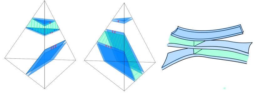
Figure 2. Thickened normal disks (blue), fibered $3$-balls (green), and the branched surface fibered neighborhood.

For any branched surface fibered neighborhood $\mathcal{N}$, its boundary decomposes into a union of three subsurfaces, the horizontal boundary $\partial_{h}\mathcal{N}$, the vertical boundary $\partial_{v}\mathcal{N}$, and $\mathcal{N}\cap\partial M$. While $\partial_{v}\mathcal{N}$ is foliated by subintervals of fibers, each $I$–fiber of $\mathcal{N}$ meets $\partial_{h}\mathcal{N}$ at its endpoints. A surface $F$ in $M$ is carried by $\mathcal{B}$ if it can be properly isotoped into the interior of a fibered neighborhood $\mathcal{N}=\mathcal{N}(\mathcal{B})$ of $\mathcal{B}$ so that it intersects each fiber transversely. It is fully carried if in addition it has nonempty intersection with each fiber. For example, $S$ is fully carried by $\widetilde{N}_{S}$ by construction.

Floyd–Oertel define a branched surface $\mathcal{B}$ to be incompressible if

1. there are no disks (or half-disks) of contact,

2. there are no complementary monogons, and

3. $\partial_{h}\mathcal{N}(\mathcal{B})$ is incompressible and $\partial$-incompressible in $M\smallsetminus\mathcal{N}(\mathcal{B})$.

Here, a disk of contact is a disk $D\subset\mathcal{N}$ that is transverse to the $I$–fibers of $\mathcal{N}$ and $\partial D\subset\mathrm{int}(\partial_{v}\mathcal{N})$. A half-disk of contact is a disk $D\subset\mathcal{N}$ that is transverse to the fibers with $\partial D=\alpha\cup\beta$, where $\alpha\smallsetminus\partial\alpha\subset\mathrm{int}(\partial_{v}\mathcal{N})$ and $\beta\subset\partial M$ are arcs and $\alpha\cap\beta=S^{0}$. A complementary monogon is a disk $D\subset M\smallsetminus\mathrm{int}(\mathcal{N})$ with $\partial D=D\cap\mathcal{N}=\alpha\cup\beta$ where $\alpha\subset\partial_{v}\mathcal{N}$ is an $I$–fiber and $\beta\subset\partial_{h}\mathcal{N}$. Floyd–Oertel show [FO84, Theorem 2] that if $\mathcal{B}$ is an incompressible branched surface, then any surface fully carried by $\mathcal{B}$ is incompressible and boundary incompressible.

Unfortunately the branched surface $\widetilde{\mathcal{B}}_{S}$ constructed above may have many disks of contact and therefore is not incompressible. However, Floyd–Oertel show that such a disk of contact $D$ may be removed by deleting from $\widetilde{\mathcal{N}}_{S}$ a fibered neighborhood of $D$ in $\widetilde{\mathcal{N}}_{S}$, thereby producing a new branched surface fibered neighborhood in which $S$ is fully carried. They prove that by applying this operation finitely many times, one can produce a fibered neighborhood $\mathcal{N}_{S}$ of an incompressible branched surface $\mathcal{B}_{S}$ [FO84, Proposition 3]. See also [Oer84, Lemma 4.6] where the construction of $\mathcal{N}_{S}$ is done more systematically. We denote the corresponding branched surface by $\mathcal{B}_{S}$ and also write $\mathcal{N}_{S}=\mathcal{N}(\mathcal{B}_{S})$.

We say that a branched surface (and its fibered neighborhod) obtained in this way is adapted to the triangulation ${\bf t}$, and record two important properties of the construction:

• Each component of $\partial_{v}\widetilde{\mathcal{N}}_{S}$ contains a subarc of the $1$-skeleton of ${\bf t}$ as a fiber of $\partial_{v}\widetilde{\mathcal{N}}_{S}$. Since eliminating a disk of contact is done by deleting a fibered neighborhood of the disk, the property that each component of $\partial_{v}\mathcal{N}$ meet the $1$-skeleton is preserved.

• The normal surface $S$, which was assumed to have minimal weight in its isotopy class, is contained in the branched surface fibered neighborhood $\mathcal{N}_{S}$, where it intersects each fiber transversely.

By Floyd–Oertel [FO84, Theorem 1] (see also [Oer84, Theorem 3]) this procedure produces a finite collection of properly embedded branched surfaces $\mathcal{B}_{1},\ldots,\mathcal{B}_{n}$ in $M$ such that $(a)$ any surface fully carried by one of the $\mathcal{B}_{i}$ is incompressible and boundary incompressible, and $(b)$ every incompressible and boundary incompressible orientable surface is fully carried by some $\mathcal{B}_{i}$. In particular, the branched surface $\mathcal{B}_{S}$ constructed from the surface $S$ appears up to isotopy as one of the $\mathcal{B}_{i}$ in this list. (That fact that $\{\widetilde{\mathcal{N}}_{S}\}$ forms a finite set of branched surfaces is obvious since there are only finitely many choices for normal disks in the construction. Showing that $\{\mathcal{N}_{S}\}$ is finite is more difficult and requires showing that one only needs to consider least weight disks of contact, of which there are finitely many.)

We summarize all of this in the following statement:

Proposition 2.7 (Floyd-Oertel).

Let $M$ be a compact Haken 3-manifold with a triangulation ${\bf t}$. There is a finite collection $\mathcal{B}_{1},\ldots,\mathcal{B}_{n}$ of incompressible properly embedded branched surfaces, so that

• Each fibered neighborhood $\mathcal{N}(\mathcal{B}_{i})$ is adapted to $\bf t$, and in particular every component of $\partial_{v}\mathcal{N}(\mathcal{B}_{i})$ has a fiber which is a subarc of an edge of ${\bf t}^{(1)}$.

• Every properly embedded incompressible boundary-incompressible surface $S$ in $M$ is properly isotopic to a surface $S^{\prime}$ fully carried in one of the $\mathcal{B}_{i}$, which realizes the minimum weight with respect to ${\bf t}$ in the isotopy class of $S$.

3. Topological preliminaries

This section covers a number of fairly basic results from $3$-manifold topology that we will need for the proof of Theorem 1.5.

3.1. Embeddings in products

We first require the following lemma, which follows easily from work of Waldhausen [Wal68].

If $S$ is a compact surface we say that $(W,\partial_{b}W)\subset(S,\partial S)$ is a subsurface with corners (or just subsurface for short) if $W$ is a compact 2-manifold and $\partial_{b}W=\partial W\cap\partial S$ is a compact 1-submanifold of $\partial W$. The endpoints of $\partial_{b}W$ are the corners and $\partial W$ minus the corners is the smooth part of $\partial W$. We denote the closure of $\partial W\smallsetminus\partial_{b}W$ as $\partial^{\prime}W$.

We call $(W,\partial_{b}W)$ (or just $W$) trivial if it is contained in a disk $D$ whose intersection with $\partial S$ is empty or a single arc. Note that if $W$ is not trivial, then either the image of $\pi_{1}W$ in $\pi_{1}S$ is nontrivial, or there is an essential arc of $S$ contained in $W$.

Define a modified Euler characteristic as

$$\hat{\chi}(W,\partial_{b}W)=\chi(W)-{1\over 2}n$$

where $n$ denotes the number of arc components of $\partial_{b}W$ (see e.g. [CB88]).

Lemma 3.1.

Suppose that $(W,\partial_{b}W)\subset(S,\partial S)$ is a subsurface with corners and that the restriction to each component of $W$ is not trivial. Let $Y=W\times[0,1]$ and suppose we have an embedding of quadruples

$$F:(Y,W\times\{0\},W\times\{1\},\partial_{b}W\times[0,1])\hookrightarrow(S\times[0,1],S\times\{0\},S\times\{1\},\partial S\times[0,1]),$$

where $W\times\{0\}\to S\times\{0\}$ is given by the inclusion map.

Then $F$ is isotopic, as a map of quadruples, to the inclusion map of $Y$.

Note that the nontriviality condition is necessary – consider a knotted 1-handle attached to two disks in $S\times\{0\}$ and $S\times\{1\}$.

Proof.

By applying a preliminary isotopy of $S\times[0,1]$ supported on a neighborhood of $\partial S\times[0,1]$, we may assume that the image of each arc of $\partial\partial^{\prime}W\times[0,1]$ is vertical in $\partial S\times[0,1]$.

If a null-homotopic closed curve $\gamma$ of $\partial^{\prime}W$ bounds a disk $E$ in $S$ then the image of $\partial(E\times[0,1])$ bounds a ball by irreducibility and $F$ can be extended over $E\times[0,1]$. Thus we may assume that each component of $W$ injects on $\pi_{1}$. Similarly if $\alpha$ is an arc component of $\partial^{\prime}W$ that cobounds a disk $E$ with an arc $\beta\subset\partial S$, we can again extend over $E\times[0,1]$. Hence, we may assume that $\partial^{\prime}W$ consists of homotopically essential curves and essential proper arcs.

Thus each component of $F(\partial^{\prime}W\times[0,1])$ is either an incompressible annulus in $S\times[0,1]$ or a disk which meets $\partial S\times[0,1]$ in two vertical arcs. Hence (see for example [Wal68, Lemma 3.4]) $F(\partial^{\prime}W\times[0,1])$ is isotopic to $\partial^{\prime}W\times[0,1]$, and we may adjust $F$ by an isotopy that is constant on $W\times\{0\}$ to obtain a map that is the identity on $\partial^{\prime}W\times[0,1]$.

One further isotopy, constant on $W\times\{0\}$ and supported on a neighborhood of $\partial_{b}W\times[0,1]$, yields a map (which we still call $F$) that is the identity on all of $\partial W\times[0,1]$.

Now $F$ is the identity on $W\times\{0\}\cup\partial W\times[0,1]$, and it follows that $F(W\times\{1\})=W\times\{1\}$, and from this that $F(Y)=Y$. Hence, by [Wal68, Lemma 3.5], the homeomorphism $F^{-1}\colon Y\to Y$ is isotopic to the identity via an isotopy that is constant on $W\times\{0\}\cup\partial W\times[0,1]$. Precomposing $F$ with this isotopy gives the required isotopy from $F$ to the identity and completes the proof. ∎

3.2. Level curves

Let $Y=Z\times I$ where $Z$ is a surface and $I$ an interval. Let $C$ be a disjoint closed union of simple loops in $\mathrm{int}(Y)$. We say $C$ is level with respect to this product structure on $Y$ if it is isotopic to a union of the form $\bigcup c_{i}\times\{t_{i}\}$ where $c_{i}$ are loops in $Z$ and $t_{i}\in[0,1]$.

Lemma 3.2.

Let $Y=Z\times[0,1]$ where $Z$ is a surface. Let $C$ be a finite union of simple loops in $Y$. Then $C$ is level if and only if there is an ordering $c_{1},\ldots,c_{n}$ of its components so that each $c_{i}$ is isotopic to $Z\times\{0\}$ in the complement of $c_{i+1}\cup\cdots\cup c_{n}$.

The proof is an easy induction.

Lemma 3.3.

Let $S$ be a compact orientable surface and let $C$ be a level disjoint closed union of essential curves in $S\times\mathbb{R}$. Let $T_{1}$ and $T_{2}$ be surfaces isotopic to $S\times\{0\}$ rel $\partial S\times\mathbb{R}$, and disjoint from each other and from $C$. If $X$ is the region bounded by $T_{1}$ and $T_{2}$ (so $X\cong S\times[0,1]$), then $C\cap X$ is level in $X$.

Furthermore, if $C\subset Y\subset X$ where $Y\subset X$ is a subproduct, then the isotopy can be chosen to be supported in $Y$—that is, the image of $C$ remains in $Y$ throughout the isotopy.

By saying that $Y$ is a subproduct of $X$ we mean that there is a subsurface $R\subset S$ and a homeomorphism of pairs $(X,Y)\cong(S\times[0,1],R\times[0,1])$.

Proof.

By applying an (ambient) isotopy, we may assume that the components of $C$ have the form $c\times\{t\}$ for some $t\in\mathbb{R}$ with respect to the given product structure on $S\times\mathbb{R}$.

We first prove this in the case that $T_{2}$ is a level surface $S\times\{t\}$. We may assume $T_{1}$ lies above $T_{2}$. Let $c$ be a component of $C\cap X$ of minimal height with respect to the product structure $S\times\mathbb{R}$. The vertical annulus $A$ taking $c$ to $T_{2}$ is disjoint from $C\setminus c$, but might intersect $T_{1}$. An innermost region of $A\cap X$ or $A\cap X^{c}$ with boundary in $T_{1}$ must be a disk or annulus, and an exchange move will simplify the intersection reducing the number of components of intersection. Thus an annulus from $c$ to $T_{2}$ meeting $T_{2}$ only in one boundary component, disjoint from $C\setminus c$, and intersecting $T_{1}$ minimally, will in fact be disjoint from $T_{1}$, hence contained in $X$. This gives an isotopy from $c$ to $T_{2}$ avoiding the remaining curves. Proceeding by induction on the heights of components of $C$, we can now apply Lemma 3.2 to conclude that $C\cap X$ is level in $X$.

Now if $T_{1}$ and $T_{2}$ are arbitrary, let $T_{3}=S\times\{t\}$ be a level surface below both. Let $X_{ij}$ be the region bounded by $T_{i}$ and $T_{j}$ and suppose $X_{13}$ contains $T_{2}$. Then the previous case applies to $X_{13}$, and after choosing a product structure on $X_{13}$ in which the top and bottom are level surfaces, we can again apply the previous case to $X_{12}$. This concludes the proof of the first claim.

Finally, suppose $C\subset Y$, with $(X,Y)\cong(S\times[0,1],R\times[0,1])$. If at any stage of the isotopy of the $i^{th}$ component the corresponding annulus passes outside $Y\cong R\times[0,1]$, and hence through $\partial R\times[0,1]$, another innermost region exchange move argument implies that we can replace the annulus with one having fewer intersections with $\partial R\times[0,1]$. In particular, such an annulus with the fewest intersections with $\partial R\times[0,1]$ will be disjoint, and hence the isotopy will be supported in $Y$. ∎

3.3. Minimal intersections

Finally, we will need a few facts regarding intersections of surfaces and $1$–manifolds. One such fact is the following proposition which roughly states that if $S$ is an embedded surface in $M$ which minimizes intersection with some $1$-manifold $C$ in its isotopy class, then one cannot homotope $S$ to reduce intersections with $C$.

Proposition 3.4.

Let $M$ be a compact, irreducible, orientable $3$-manifold and $C\subset M$ is a closed, embedded $1$–manifold. Suppose $S\subset M$ is an incompressible, boundary incompressible, properly embedded surface that minimizes the cardinality $|S\cap C|$ in its proper isotopy class. If $f\colon S\to M$ is any piecewise smooth map which is properly homotopic to the inclusion of $S$ and transverse to $C$, then $|f^{-1}(C)|\geq|S\cap C|$.

Proof.

Suppose $f\colon S\to M$ is any piecewise smooth map properly homotopic to the inclusion of $S$ into $M$, and which is transverse to $C$. Set $k=|f^{-1}(C)|$. Let $V_{C}\cong C\times D^{2}$ be a small tubular neighborhood of $C$. Adjusting $f$ by a proper homotopy, we may assume that $f(S)\cap V_{C}$ is a union of $k$ disjoint meridian disks. Next let $N\cong\partial M\times[0,1)$ be a tubular neighborhood of the boundary of $M$ whose closure is disjoint from $V_{C}$. Using the neighborhood $N$ and the homotopy from the inclusion of $S$ to $f$, we can find a further homotopy so that $f|_{\partial S}$ is the inclusion $\partial S\to\partial M$ (and is hence an embedding) and so that $f(S)\cap V_{C}$ is still a union of $k$ disjoint meridian disks.

Next, choose any Riemannian metric on $M$ with the following properties:

1. the restriction to $V_{C}\cong C\times D^{2}$ is a product metric,

2. the restriction to $N\cong\partial M\times[0,1)$ is a product metric,

3. the area of each meridian disk of $V_{C}$ is some number $A>0$, and

4. $\mathrm{Area}(f)\leq(k+\frac{1}{4})A$.

It is straightforward to construct such a metric.

Now let $h\colon S\to M$ be a least area surface properly homotopic to the inclusion of $S$ into $M$ rel $\partial S$. Such an $h$ exists by [SU82, SY79] in the closed case and [Lem82, HS88] in the case of non-empty boundary. Note that $\mathrm{Area}(h)\leq(k+\frac{1}{4})A$.

According to [FHS83], $h$ is an embedding, or in the case that $S$ is closed, possibly a double cover an embedded non-orientable surface with a tubular neighborhood that is a twisted $I$–bundle over the non-orientable surface (see Section 7 of [FHS83] for the case $\partial S\neq\emptyset$). In the latter case, we may replace $h$ with an embedding at the expense of an arbitrarily small increase in the area. In either case, by a further small isotopy if necessary, we can also assume that $h$ is transverse to $\partial V_{C}$ and $\mathrm{Area}(h)\leq(k+\frac{1}{2})A$. The embedding $h$ is properly isotopic to the inclusion of $S$ into $M$ since $M$ is irreducible [Wal68, Corollary 5.5].

Consider any component $W$ of $h(S)\cap V_{C}$ and suppose $V\cong S^{1}\times D^{2}$ is the component containing $W$.

Note that the projection $V\to D^{2}$ onto the second factor is an isomorphism $H_{2}(V,\partial V)\to H_{2}(D^{2},\partial D^{2})$, where the latter group is $\mathbb{Z}[D^{2}]$. Thus we can define $\deg(W)$ to be the integer such that

$$[W]=\deg(W)[D^{2}]\in H_{2}(V,\partial V).$$

This is equal to the topological degree of the projection $(W,\partial W)\to(D^{2},\partial D^{2})$, as well as the topological degree of the map $\partial W\to\partial D^{2}$.

Now consider the metric on $D^{2}$ for which the projection $V\to D^{2}$ is a Riemannian submersion, and in particular a contraction. We thus have

$$\mathrm{Area}(W)\geq|\deg(W)|A.$$

Setting

$$d(h)=\sum_{W\subset h(S)\cap V_{C}}|\deg(W)|$$

where the sum is over all components of intersection, and combining with our area bound on $h$, we have

$$d(h)A\leq\mathrm{Area}(h)\leq(k+\frac{1}{2})A.$$

Since $d(h)$ is an integer, we have $d(h)\leq k$. The next claim essentially completes the proof.

Claim 1.

The map $h$ is properly isotopic to an embedding $h^{\prime}$, transverse to $\partial V_{C}$ with $d(h^{\prime})\leq d(h)$ so that $h^{\prime}(S)\cap V_{C}$ is a union of meridian disks.

Assuming the claim, it follows that $|h^{\prime}(S)\cap C|$ is the number of meridian disks of intersection $h^{\prime}(S)\cap V_{C}$, which is $d(h^{\prime})\leq d(h)\leq k$. Since $S$ was assumed to meet $C$ in the fewest number of points in the proper isotopy class, and since $h^{\prime}$ is properly isotopic to $h$, and hence also the inclusion of $S$, it follows that

$$|S\cap C|\leq d(h^{\prime})\leq k=|f^{-1}(C)|,$$

as required. This completes the proof of the proposition.

Proof of Claim.

Recall first a lemma of Thurston [Thu86b, Lemma 1], that if a properly embedded surface in a 3-manifold $V$ represents a $k$-th multiple of a homology class in $H_{2}(V,\partial V)$, then the surface has at least $k$ components. Thus for our connected components $W$ of $h(S)\cap V_{C}$, we have

$$|\deg(W)|\leq 1.$$

To avoid cluttering the notation, we write $S_{0}=h(S)$, $d(S_{0})=d(h)$. Throughout the proof, we repeatedly replace $S_{0}$ with isotopic images which we again denote $S_{0}$. We first isotope $S_{0}$ to remove trivial intersections with $\partial V_{C}$. That is, if some component of $S_{0}\cap\partial V_{C}$ bounds a disk $D$ in $\partial V_{C}$, then it also bounds a disk $E$ in $S_{0}$ by incompressibility. Suppose that $D$ is innermost on $\partial V_{C}$, and consider the disk swap that replaces the disk $E$ in $S_{0}$ with $D$. (This can be done via isotopy of $S_{0}$ in $M$ since $D\cup E$ bounds a ball.) This may reduce the number of intersections with $V_{C}$, but it does not increase $d(S_{0})$. To see this, note that if $W$ was the component of $S_{0}\cap V_{C}$ whose boundary contained $\partial D$, then since $\partial D\to\partial D^{2}$ has degree $0$, the degree of $W$ is unaffected by capping this boundary component off with the disk $D$. After pushing $D$ slightly into $V_{C}$, we have a new surface isotopic to $S_{0}$ with fewer trivial intersections with $\partial V_{C}$ and no greater degree.

Hence, we may suppose that $S_{0}$ does not meet $\partial V_{C}$ in trivial circles. We next isotope $S_{0}$ so that each component of $S_{0}\cap V_{C}$ is incompressible: If $D$ is a compressing disk for some component $W$ of $S_{0}\cap V_{C}$, then again suppose that $D$ is innermost in the sense that $S_{0}$ does not meet the interior of $D$. Incompressibility of $S_{0}$ in $M$ implies that there is a disk $E\subset S_{0}$ with $\partial E=\partial D$ and we may assume that $E$ is not contained in $V_{C}$.

Let $W$ be the component of $S_{0}\cap V_{C}$ meeting $D$. Compressing along $D$ results in two surfaces $W_{1}$ and $W_{2}$ and we call $S_{0}^{\prime}$ the surface isotopic to $S_{0}$ obtained by replacing $E$ with $D$ (again possible since $D\cup E$ bounds a ball). Label so that $W_{1}$ is a component of $S_{0}^{\prime}\cap V_{C}$. Let $\mathcal{Y}$ be the components of $S_{0}\cap V_{C}$ contained in $S_{0}\smallsetminus E$ and $\mathcal{Z}$ the components of $S_{0}\cap V_{C}$ contained in $E$. Then

$$d(S_{0})=\sum_{Y\in\mathcal{Y}}|\deg(Y)|+|\deg(W)|+\sum_{Z\in\mathcal{Z}}|\deg(Z)|$$

and

$$d(S_{0}^{\prime})=\sum_{Y\in\mathcal{Y}}|\deg(Y)|+|\deg(W_{1})|.$$

We must show that $d(S_{0}^{\prime})\leq d(S_{0})$. Since $|\deg(W_{1})|$ and $|\deg(W)|$ are both at most 1, it suffices to prove that there is at least one $Z\in\mathcal{Z}$ with $|\deg(Z)|=1$.

Let $E^{\prime}$ be an innermost disk on $E$ bounded by a component of $E\cap\partial V_{C}$. Then $\partial E^{\prime}$ is an essential curve on the boundary of some component of $V_{C}$. If $\mathrm{int}(E^{\prime})$ is in the exterior of $V_{C}$ then $\partial V_{C}$ is compressible in $\mathring{M}$, and this is impossible as $\mathring{M}$ is hyperbolic. Thus $E^{\prime}$ is a meridian of $V_{C}$, which implies it is a component of $\mathcal{Z}$ with $|\deg(E^{\prime})|=1$.

Thus we have isotoped $S_{0}$ to reduce intersections with $\partial V_{C}$ while not increasing its degree. We may therefore assume that each component of $S_{0}\cap V_{C}$ is incompressible in $V_{C}$. This makes each component either a boundary parallel annulus (degree $0$) or a meridian disk (degree $\pm 1$). Pushing the annuli out of $V_{C}$ does not affect the degree and completes the proof. ∎

∎

4. Fibered fillings of manifolds

In this section we prove Theorem 1.5 and Theorem 1.4. After setting up notation for Dehn filling and bringing in the branched surfaces from Section 2.4, we begin the proof in earnest in Section 4.4.

4.1. Fillings and complexity

Let $\mathring{M}$ be a compact $3$-manifold whose boundary is a union of tori $\partial\mathring{M}=\partial_{1}\mathring{M}\sqcup\cdots\sqcup\partial_{r}\mathring{M}$, such that $\mathrm{int}(\mathring{M})$ is a complete finite-volume hyperbolic manifold. A Dehn surgery coefficient $\beta_{i}$ on $\partial_{i}\mathring{M}$ is either the isotopy class of an essential simple closed curve in $\partial_{i}\mathring{M}$, or “$\infty$”. Each simple closed curve $\beta_{i}$ in $\partial_{i}\mathring{M}$ determines a Dehn filling attaching a solid torus whose meridian is identified with $\beta_{i}$, and $\infty$ corresponds to no filling at all. Given $\beta=(\beta_{1},\ldots\beta_{r})$, we denote the manifold obtained by these specified fillings by $M_{\beta}$.

Letting $\Delta_{i}$ denote the set of Dehn surgery coefficients for $\partial_{i}\mathring{M}$, we say that a property $\mathcal{P}$ holds for all sufficiently long fillings if there are finite sets $K_{i}\subset\Delta_{i}$ that that $M_{\beta}$ has $\mathcal{P}$ for all $\beta\in\prod_{i=1}^{r}(\Delta_{i}\smallsetminus K_{i})$. For example, Thurston’s hyperbolic Dehn surgery theorem [Thu88, Theorem 5.8.2] states that for any $\ell>0$, the interior of $M_{\beta}$ is hyperbolic and the lengths of the cores of the filled solid tori are less than $\ell$, for all sufficiently long fillings.

Now let $\mathring{M}$ be as in the statement of Theorem 1.5 and let $\SS$ be the collection of all fibers of all fibered fillings of $\mathring{M}$. (Formally $\SS$ is a set of pairs $(S,\beta)$ where $\beta$ determines a filled manifold $M_{\beta}$ in which $S$ is a fiber of a fibration.) Note that we do not require each boundary component of $\mathring{M}$ to be filled, so some surfaces in $\SS$ may have boundary. We also fix a triangulation ${\bf t}$ of $\mathring{M}$.

Given $(S,\beta)\in\SS$, isotope $S$ in $M_{\beta}$ to intersect the added solid tori in meridian disks, and choose it so the number of disks is minimal. Now let $\mathring{S}=S\cap\mathring{M}$, and assume by further isotopy if necessary, that $\mathring{S}$ is also transverse to ${\bf t}^{(1)}$ and intersects it minimally. Let $\mathring{\SS}=\{\mathring{S}:(S,\beta)\in\SS\}$ denote the resulting set of properly embedded surfaces in $\mathring{M}$. Said differently, for each $(S,\beta)\in\SS$, $\mathring{S}$ is a properly embedded surface in $\mathring{M}$ which after capping off with a disk is isotopic in $M_{\beta}$ to $S$ and, among all such surfaces, minimize the complexity defined by the pair $(|\partial\mathring{S}|,w(\mathring{S}))$ in the lexicographic order, where $w(\mathring{S})$ is the weight of $\mathring{S}$.

Lemma 4.1.

Each $\mathring{S}\in\mathring{\SS}$ is incompressible and boundary incompressible in $\mathring{M}$.

Proof.

The proof is standard, but we sketch it for completeness.

Suppose that $\mathring{S}$ is compressible and let $D$ be a compressing disk for $\mathring{S}$ in $\mathring{M}$. Since $S$ is incompressible in its filling $M_{\beta}$, this disk shares a boundary with a disk $D^{\prime}$ in $S$, which must meet the cores of the filling tori. Swapping out $D^{\prime}$ for $D$, which can be done by an isotopy in $M_{\beta}$, results in a copy of $S$ meeting the cores of the solid tori fewer times, a contradiction. Hence, $\mathring{S}$ is incompressible.

Now if $\mathring{S}$ is boundary-compressible let $E$ be a boundary compression, so that $\partial E$ is the union of an arc $b$ in $\mathring{S}$ and an arc $a$ in $\partial\mathring{M}$. Then $a$ is contained in an annular component $A$ of $\partial\mathring{M}\smallsetminus\partial\mathring{S}$, and it must be essential there since otherwise $E$ is not an essential boundary compression. Now $A$ cut along $a$ and attached to two parallel copies of $E$ gives us a compressing disk for $\mathring{S}$, which therefore is parallel to a disk of $\mathring{S}$ by incompressibility. But this disk, attached to itself along $b$, forms an annulus which must be all of $\mathring{S}$, so that $\mathring{S}$ is a boundary-parallel annulus. This is a contradiction. ∎

Now Proposition 2.7 gives us a finite collection $\mathcal{B}_{1}\ldots,\mathcal{B}_{n}$ of incompressible branched surfaces in $\mathring{M}$ so that each $\mathring{S}\in\mathring{\SS}$ is fully carried in a weight-minimizing way in one of them.

For each $\mathcal{B}_{i}$ let $\SS_{\mathcal{B}_{i}}$ contain those $(S,\beta)\in\SS$ for which $\mathring{S}$ is fully carried by $\mathcal{B}_{i}$. After restricting to “sufficiently long” fillings in this collection, we can make some additional assumptions about $\mathcal{B}_{i}$:

Let $T_{j}$ be a component of $\partial\mathring{M}$. If, for $(S,\beta)\in\SS_{\mathcal{B}_{i}}$, the coordinate $\beta_{j}$ only takes on finitely many values, we can exclude all of the non-$\infty$ values in our definition of sufficiently long. Then unless $\infty$ is also one of the values, we can ignore $\mathcal{B}_{i}$ altogether.

Thus we can assume that for each boundary component $T_{j}$ of $\mathring{M}$ meeting $\mathcal{B}_{i}$, either the fibers of $\SS_{\mathcal{B}_{i}}$ determine infinitely many slopes in $T_{j}$ or $T_{j}$ is not filled in any of the fillings corresponding to $\SS_{\mathcal{B}_{i}}$. In particular, this means that each boundary torus $T_{j}$ of $\partial\mathring{M}$ is either disjoint from $\mathcal{B}_{i}$, meets it in a train track and the complements of these tracks are bigons, or meets $\mathcal{B}_{i}$ in a disjoint union of parallel simple closed curves in $T_{i}$ whose complement is a union of annuli. In the last case $\beta_{j}=\infty$ for all $(S,\beta)\in\SS_{\mathcal{B}_{i}}$ with $\beta$ sufficiently long.

4.2. Branched surface decomposition

From here on, we work with a single $\mathcal{B}=\mathcal{B}_{i}$, restricted as above. The notion of “sufficiently long filling” will depend on the particular branched surface $\mathcal{B}$, but finiteness of the number of branched surfaces provides a uniform notion of sufficiently long filling, independent of $\mathcal{B}$. We continue to write $\mathcal{N}=\mathcal{N}(\mathcal{B})$ for the fibered neighborhood of $\mathcal{B}$ in $\mathring{M}$.

Divide $\partial\mathring{M}$ into the tori that meet $\mathcal{B}$ – called $\partial^{B}\mathring{M}$ – and the rest, $\partial^{F}\mathring{M}$ ($F$ for “floating”).

Given $(S,\beta)\in\SS_{\mathcal{B}}$, let $V_{\beta}$ be the union of solid tori associated to the fillings, $M_{\beta}=\mathring{M}\cup V_{\beta}$. We write $V_{\beta}^{B}$ and $V_{\beta}^{F}$ for the solid tori that meet and do not meet $\mathcal{B}$, respectively. We remark that $\partial V_{\beta}^{F}=\partial^{F}\mathring{M}$ and $\partial V_{\beta}^{B}\subset\partial^{B}\mathring{M}$ with this containing being proper if there are unfilled boundary components of $\mathring{M}$ for $\beta$.

Now let $X=\mathring{M}\smallsetminus\mathcal{N}(\mathcal{B})$ and set $X_{\beta}=X\cup V_{\beta}^{F}$. We divide $\partial X_{\beta}$ into $\partial X_{\beta}=\partial_{h}X_{\beta}\cup\partial_{v}X_{\beta}$, where $\partial_{h}X_{\beta}=\partial_{h}\mathcal{N}$, and $\partial_{v}X_{\beta}$ consists of annuli which are either annulus components of $\partial_{v}\mathcal{N}$, annulus components of $X\cap\partial\mathring{M}$, or unions of rectangle components of $\partial_{v}\mathcal{N}$ with bigon regions in $\partial\mathring{M}\smallsetminus\mathcal{N}$. We similarly decompose $\partial X=\partial_{h}X\cup\partial_{v}X$, where $\partial_{h}X=\partial_{h}X_{\beta}$, and $\partial_{v}X=\partial_{v}X_{\beta}\cup\partial^{F}\mathring{M}$.

The foliation by interval fibers of $\mathcal{N}(\mathcal{B})$ extends first to a foliation on each of the non-floating boundary tori $\partial^{B}\mathring{M}$; this is because the complement of $\partial_{v}\mathcal{N}$ in $\partial^{B}\mathring{M}$ is a union of bigons and annuli. For each $\beta$, the meridians are transversal to this foliation so it extends to a foliation of the solid tori $V^{B}_{\beta}$, which is transverse to (a fixed family of) meridian disks.

Call the resulting foliation $\mathcal{I}$, and note that it is defined in $M_{\beta}\smallsetminus\mathrm{int}(X_{\beta})=\mathcal{N}\cup\partial^{B}\mathring{M}\cup V^{B}_{\beta}$.

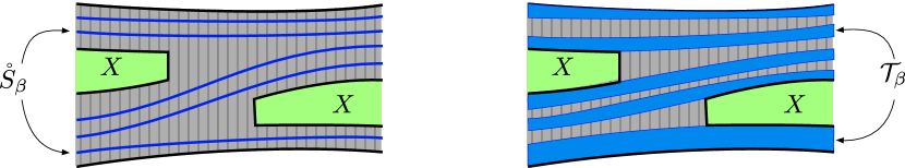
Figure 3. Left: $\mathring{S}_{\beta}$ is carried by $\mathcal{N}$. Right: $S_{\beta}$ is thickened to the $I$-bundle $\mathcal{T}_{\beta}$ (blue). The $I$-foliation is shown in the complementary part of $\mathcal{N}$, which is part of $\mathcal{F}_{\beta}$.

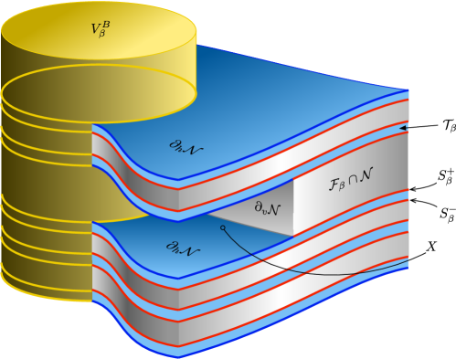
Figure 4. A cutaway view of $\mathcal{N}$ near a component of $V^{B}_{\beta}$. The $I$-bundle $\mathcal{T}_{\beta}$ is indicated in blue inside $\mathcal{N}$ and the complementary $I$-bundle $\mathcal{F}_{\beta}$ is in gray. The surfaces $S^{\pm}_{\beta}$ are indicated with blue edges in $\partial_{h}\mathcal{N}$, with yellow along the meridians, and with red edges in the remainder $W_{\beta}$.

4.3. Product regions in $M_{\beta}$

Fix $(S,\beta)\in\SS_{\mathcal{B}}$, and for convenience denote $S$ by $S_{\beta}$. We can realize $S_{\beta}$ as a surface contained in $\mathcal{N}(\mathcal{B})$ union the solid tori $V_{\beta}^{B}$, in which it is transverse to the foliation $\mathcal{I}$. Thicken $S_{\beta}$ to make a product $I$-bundle $\mathcal{T}_{\beta}$ with $I$–fibers being arcs of leaves of $\mathcal{I}$, then isotope $\mathcal{T}_{\beta}$ so that its boundary contains $\partial_{h}\mathcal{N}(\mathcal{B})$. This is done by pushing the boundary surfaces outward along $\mathcal{I}$-leaves until they touch the endpoints. See Figure 3 for a schematic of this, and Figure 4 for a 3-D view near a component of $V_{\beta}$.

Let $\mathcal{F}_{\beta}$ be the closure of $M_{\beta}\smallsetminus\mathcal{T}_{\beta}$. Since $S_{\beta}$ is a fiber of $M_{\beta}$, $\mathcal{F}_{\beta}$ is also a product $I$-bundle. We use the $I$-bundle structure to define $\partial_{v}$ and $\partial_{h}$ for both $\mathcal{F}_{\beta}$ and $\mathcal{T}_{\beta}$, writing

$$\partial_{h}\mathcal{F}_{\beta}=\partial_{h}\mathcal{T}_{\beta}=S_{\beta}^{+}\sqcup S_{\beta}^{-},$$

and noting that $\partial_{v}\mathcal{F}_{\beta}\cup\partial_{v}\mathcal{T}_{\beta}=\partial M_{\beta}$.

Note that $\mathcal{F}_{\beta}$ contains $X_{\beta}$, $\mathcal{F}_{\beta}\smallsetminus X_{\beta}$ is contained in $\mathcal{N}\cup V^{B}_{\beta}$, and the foliation $\mathcal{I}$ restricts to a foliation $\mathcal{I}|(\mathcal{F}_{\beta}\smallsetminus X_{\beta})$. Hence, $\mathcal{F}_{\beta}$ decomposes into the ‘$I$-foliated part’ $\mathcal{I}|(\mathcal{F}_{\beta}\smallsetminus X_{\beta})$ and the ‘bounded part’ $X_{\beta}$, as anticipated by our discussion in Section 1.1.

Our main goal now is to show that $\mathcal{I}|(\mathcal{F}_{\beta}\smallsetminus X_{\beta})$ is (up to isotopy) also the restriction of the product interval foliation on $\mathcal{F}_{\beta}\cong S_{\beta}\times[0,1]$. For a summary of our strategy, see the outline in Section 1.1. From this we will deduce that $\mathcal{I}$ is the foliation by flow lines of the suspension flow for the monodromy of the fiber $S_{\beta}$ of the given fibration of $M_{\beta}$. This is completed in Proposition 4.6.

4.4. Regions in $\partial_{h}\mathcal{F}_{\beta}$ and hyperbolic geometry

Let $W_{\beta}$ denote the closure of $\partial_{h}\mathcal{F}_{\beta}\smallsetminus\partial_{h}X$. Note that $W_{\beta}$ is the union of the meridian disks $\mathcal{D}_{\beta}=\partial_{h}\mathcal{F}_{\beta}\cap V_{\beta}^{B}$ and regions that are contained in the interior of $\mathcal{N}(\mathcal{B})$.

Note that $\partial_{h}X$ is a subsurface with corners in $\partial_{h}\mathcal{F}_{\beta}\cap\mathring{M}$ in the sense of Section 3.1 – it is bounded by circles and arcs whose endpoints are on the circles of $\partial_{h}\mathcal{F}_{\beta}\cap\partial\mathring{M}$ – some of which are boundaries of the meridian disks and some can be in $\partial M_{\beta}$ itself, when that is nonempty. See Figures 5 and 6 for some example local configurations.

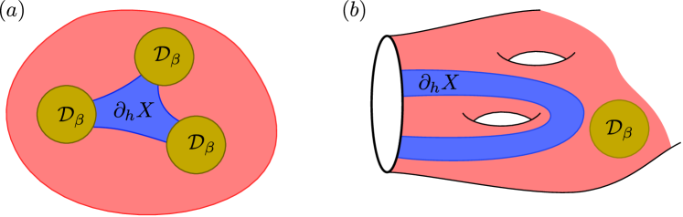
Figure 5. Examples of the decomposition of $\partial_{h}\mathcal{F}_{\beta}$. $W_{\beta}$ is the union of red and the yellow meridians. (a) shows a component of $W_{\beta}$ of low complexity containing meridians, which is ruled out for long fillings by Lemma 4.2. (b) shows part of a larger component of $W_{\beta}$ adjacent to the boundary of $M_{\beta}$.

For any component $E$ of $W_{\beta}$, let $\hat{E}$ denote the union of $E$ with any disks of $\partial_{h}\mathcal{F}_{\beta}\smallsetminus\mathrm{int}(E)$ that meet $\partial(\partial_{h}\mathcal{F}_{\beta})$ in at most one arc. Note that $E$ and $\hat{E}$ are subsurfaces with corners of $\partial_{h}\mathcal{F}_{\beta}$ in the sense of Section 3.1.

Lemmas 4.2 and 4.4 restrict the structure of components of $W_{\beta}$ for sufficiently long fillings.

Lemma 4.2.

Fix an integer $k$. For all sufficiently long fillings, if $E$ is a component of $W_{\beta}$ with $\hat{\chi}(\hat{E})=k$, then $\hat{E}$ is disjoint from $\mathcal{D}_{\beta}$.

Here $\hat{\chi}$ is modified Euler characteristic as in Section 3.1.

Proof.

Consider first those $\beta$ for which $\partial M_{\beta}=\emptyset$, in which case $\partial_{h}\mathcal{F}_{\beta}$ is a closed surface and $\hat{\chi}(\hat{E})=\chi(\hat{E})$.

Identify $\mathring{M}$ once and for all with the complement of some standard cusps in the finite-volume hyperbolic metric on $\mathrm{int}(\mathring{M})$. Thurston’s Dehn filling theorem tells us that $\mathring{M}$ embeds nearly isometrically in the hyperbolic structure on $M_{\beta}$, for sufficiently long fillings, so that its complement $\mathrm{int}(V_{\beta})$ consists of the Margulis tubes for the corresponding curves. Moreover the radii of these tubes are arbitrarily large for sufficiently long fillings $\beta$. Note that $\partial\hat{E}$ is contained in $\partial\partial_{h}X$, which is independent of $\beta$. There is therefore some bound $\kappa$, independent of $\beta$, on the total curvature of $\partial\hat{E}$ in $M_{\beta}$.

Fix a triangulation of $\hat{E}$ with vertices on the boundary so that each triangle has at most one edge on the boundary. For each $\beta$ let $f_{\beta}\colon\hat{E}\to M_{\beta}$ be a map which is a ruled surface on each triangle and is homotopic rel boundary to the inclusion map. Then the Gauss-Bonnet theorem for the induced metric on $f_{\beta}(\hat{E})$ gives us

$$\mathrm{Area}(f_{\beta}(\hat{E}))\leq-2\pi\chi(\hat{E})+\kappa.$$

Note that the right hand side is independent of $\beta$.

The following lemma (whose proof appears below) now allows us to finish the proof:

Lemma 4.3.

Given $A\geq 0$ there is an $R\geq 0$ such that the following holds. Let $V$ be a hyperbolic Margulis tube of radius $R$ and let $W$ be a compact, connected, oriented surface with a map $f\colon(W,\partial W)\to(V,\partial V)$ such that $\mathrm{Area}(f(W))<A$. Then $f$ is homotopic rel $\partial W$ into $\partial V$.

Applying this to each intersection of $f_{\beta}(\hat{E})$ with the Margulis tubes $V_{\beta}$, and choosing $\beta$ long enough to give the needed value for the tube radii, we find that we can homotope $\partial_{h}\mathcal{F}_{\beta}$ in $M_{\beta}$ (and hence $S_{\beta}$ in $M_{\beta}$) to remove its intersections with the cores of $V_{\beta}$ that occur in $\hat{E}$. Since $S_{\beta}$ was already chosen to minimize these intersections in its isotopy class, and Proposition 3.4 says that it must also minimize them in its homotopy class, we conclude that $\hat{E}$ could not in fact have contained any meridian disks.

Now consider those $\beta$ for which some specific set of coordinates is $\infty$. The corresponding tori are unfilled so $\partial M_{\beta}$ is nonempty, and each component is associated to a cusp in $M_{\beta}$. We adapt the argument to handle these cusps.

We identify $M_{\beta}^{\partial}\equiv\mathring{M}\smallsetminus\partial M_{\beta}$ with the complement of the remaining standard cusps in the finite-volume hyperbolic structure on $\mathrm{int}(\mathring{M})$. Again for sufficiently long fillings we can embed this nearly isometrically in the hyperbolic structure on $\mathrm{int}(M_{\beta})$ as the complement of the Margulis tubes of the filled boundary components.

Let $\hat{E}_{\beta}=\hat{E}\cap M^{\partial}_{\beta}$, which is $\hat{E}$ minus the arcs and curves of its boundary that lie in $\partial M_{\beta}$. We can (after suitable isotopy of the hyperbolic metric) assume that the boundary arcs of $\hat{E}_{\beta}$ are, in some neighborhood of the boundary, totally geodesic rays exiting the cusps. Thus the ends of $\hat{E}_{\beta}$ can be deformed to finite-area cusps or “spikes” (regions between two asymptotic geodesics).

Now our triangulation of $\hat{E}_{\beta}$ can be chosen with an ideal vertex at each end of the surface, and when we homotope it rel boundary (and rel ideal boundary points) to a ruled surface, the Gauss-Bonnet theorem applies again, but with an additional $\pi$ in the boundary term for each spike. Thus we have

$$\mathrm{Area}(f_{\beta}(\hat{E}_{\beta}))\leq-2\pi\hat{\chi}(\hat{E})+\kappa.$$

Lemma 4.3 again applies, allowing us for sufficiently long fillings to find a proper homotopy of $\hat{E}_{\beta}$ rel boundary and rel ends which removes all intersections of $\hat{E}$ with $V_{\beta}$. A standard argument in the collar of $\partial M_{\beta}$ allows us to obtain a homotopy of $\hat{E}$ itself which does the same thing. Again we conclude that $\hat{E}$ could not have contained any meridian disks. ∎

We now supply the proof of Lemma 4.3.

Proof.

We can write $V=D^{2}\times S^{1}$, where $D^{2}\times\{t\}$ are totally geodesic meridian disks for $t\in S^{1}$, and let $p:V\to D^{2}$ be the projection, in such a way that $p$ is area preserving on the meridian disks.

We can write the area form of the meridian disks of $V$ explicitly in cylindrical coordinates $(r,\theta,z)$ in the universal cover of $V$, namely $\alpha=\sinh r\,dr\wedge d\theta$. Note that this is closed, and evaluates to $2\pi(\cosh R-1)$ on a meridian disk. Thus $\alpha$ represents $2\pi(\cosh R-1)p^{*}(\eta)$ where $\eta$ is the fundamental class of $H^{2}(D^{2},\partial D^{2})$.

Now the map $(p\circ f)_{*}:H_{2}(W,\partial W)\to H_{2}(D^{2},\partial D^{2})$ is just multiplication by an integer, the degree $\deg(p\circ f)$. We can therefore compute this degree by integrating $\alpha/2\pi(\cosh R-1)$. That is,

$$\deg(p\circ f)={1\over 2\pi(\cosh R-1)}\int_{W}f^{*}\alpha.$$

On the other hand, because (fiberwise) orthogonal projection in the tangent bundle of $V$ to the meridian disk direction is contracting, we also have

$$\left|\int_{W}f^{*}\alpha\right|\leq\mathrm{Area}(f(W))<A.$$

Thus we have

$$|\deg(p\circ f)|<A/2\pi(\cosh R-1).$$

Since the degree is an integer, for suitably large $R$ we conclude $\deg(p\circ f)=0$.

Now a relative version of the Hopf Degree Theorem (see for example the Extension Theorem in [GP10, Chapter 3]) tells us that, since $\deg(p\circ f)=0$, there is a homotopy $G$ rel $\partial W$ taking $p\circ f$ to a map $g$ that takes values in $\partial D^{2}$. Writing $f=(f_{1},f_{2})$ where $f_{1}=p\circ f$ and applying the homotopy $G$ to the first coordinate completes the proof. ∎

Recall from Section 3.1 that a component of $W_{\beta}$ is called trivial if it is contained in a disk $D$ which is either contained in the interior of $S_{\beta}^{\pm}$ or meets $\partial S_{\beta}^{\pm}$ in a single arc. Note that if a component $E$ of $W_{\beta}$ is not trivial, then $\partial\hat{E}\smallsetminus\partial S_{\beta}^{\pm}$ consists of homotopically essential curves and essential proper arcs in $S_{\beta}^{\pm}$.

Lemma 4.4.

For sufficiently long fillings, $W_{\beta}$ has no trivial components.

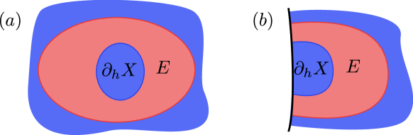
Figure 6. Two trivial components of $W_{\beta}$ which result in a disk and half-disk of contact.

Proof.

First suppose that a component $E$ of $W_{\beta}$ were contained in a disk that does not meet $\partial(\partial_{h}\mathcal{F}_{\beta})$. Then $E$ would be a (possibly punctured) disk, so $\hat{E}\subset\partial_{h}\mathcal{F}_{\beta}$ would also be a disk not meeting $\partial(\partial_{h}\mathcal{F}_{\beta})$.

Lemma 4.2 implies that for sufficiently long fillings, $\hat{E}$ (and hence $E$) contains no meridians. In particular $\partial\hat{E}$ must be a smooth boundary component of $\partial_{h}X$ (as in Figure 6(a)). That is, $\hat{E}\subset\mathcal{N}$ and $\partial\hat{E}\subset\partial_{v}\mathcal{N}$. But then, as in [FO84, Claim 1], we can isotope $\hat{E}$ to slide $\partial\hat{E}$ into $\mathrm{int}(\partial_{v}\mathcal{N})$ thereby producing a disk of contact for $\mathcal{B}$. See Figure 7.

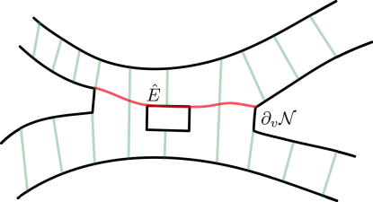
Figure 7. A disk $\hat{E}$ (red) in $\mathcal{N}$ with boundary in $\partial_{v}\mathcal{N}$. Sliding $\partial\hat{E}$ slightly downward produces the disk of contact.

This is a contradiction and the proof is complete in this case.

If instead $E$ were contained in some disk in $\partial_{h}\mathcal{F}_{\beta}$ which meets $\partial(\partial_{h}\mathcal{F}_{\beta})$ in a single arc, then $\hat{E}$ would also be a disk whose boundary has a single arc in common with $\partial(\partial_{h}\mathcal{F}_{\beta})$ (as in Figure 6(b)). Just as in the previous case, Lemma 4.2 implies that $\hat{E}$ contains no meridians and so is contained in $\mathcal{N}$. This time since $\partial E$ consists of one arc in $\partial\mathring{M}$ and one arc in $\partial_{v}\mathcal{N}$ we see that $\hat{E}$ produces a half-disk of contact for $\mathcal{B}$ and also results in a contradiction. ∎

4.5. Transverse orientability of $\mathcal{B}$

Lemma 4.5.

The branched surface $\mathcal{B}$ is transversely orientable. Equivalently, the foliation $\mathcal{I}$, defined on $M_{\beta}\setminus X_{\beta}=\mathcal{N}(\mathcal{B})\cup V^{B}_{\beta}$, is orientable.

Transverse orientability of $\mathcal{B}$ is clearly equivalent to the orientability of the foliation of $\mathcal{N}=\mathcal{N}(\mathcal{B})$ by $I$–fibers. Any orientation on this foliation of $\mathcal{N}$ easily extends to an orientation of the foliation $\mathcal{I}$.

The proof is an adaptation of an argument of Oertel [Oer86] who proved that branched surfaces constructed from Thurston-norm minimizing surfaces are transversely orientable. In our case we appeal to the notion of complexity defined in Section 4.1 and minimization in an isotopy class, rather than Thurston’s complexity, $\chi_{-}$, minimized over a homology class.

Proof.

Suppose $\mathcal{B}$ is not transversely orientable. Let $(S_{\beta},\beta)\in\SS_{\mathcal{B}}$, and fix a transverse orientation on $S_{\beta}$, and hence on $\mathring{S}_{\beta}$. We will show that, for sufficiently long $\beta$, this leads to a contradiction.

Since $\mathring{S}_{\beta}$ is fully carried on $\mathcal{B}$ there must be a branch of $\mathcal{B}$ where the orientations are inconsistent. So there is a region in $\mathcal{N}$ where there are two adjacent sheets of $\partial_{h}\mathcal{F}_{\beta}$ whose transverse orientations point into (or out of) the region of $\mathcal{F}_{\beta}$ between them. Extending this region maximally along $\mathcal{F}_{\beta}\smallsetminus\mathrm{int}(X_{\beta})$, one obtains a subset of $\mathcal{F}_{\beta}$ of the form $P\cong E\times[0,1]$ where $E\times\{0\}$ and $E\times\{1\}$ are identified with components $E_{0}$ and $E_{1}$ of $W_{\beta}$ on the same component of $\partial_{h}\mathcal{F}_{\beta}$, which we denote $S_{\beta}^{+}$ without loss of generality.

Just as at the beginning of the proof of Lemma 3.1, if $\hat{E}_{0}\neq E_{0}$ then we can extend the product region $P$ to $\hat{P}\cong\hat{E}\times[0,1]$ such that $\hat{E}\times\{0\}$ and $\hat{E}\times\{1\}$ are identified with $\hat{E}_{0}$ and $\hat{E}_{1}$. In a bit more detail, any disk $D_{0}$ of $\hat{E}_{0}\smallsetminus E_{0}$ corresponds to a disk $D_{1}$ in $\hat{E}_{1}\smallsetminus E_{1}$ (by incompressibility and boundary incompressibility of $S_{\beta}^{+}$ in $\mathcal{F}_{\beta}$) and these disks, along with a foliated annulus of $P$, cobound a ball in $\mathcal{F}_{\beta}$ (by irreducibility of $\mathcal{F}_{\beta}$). Each such ball can be foliated with intervals, extending the foliation of $P$, and $\hat{P}$ is the subset of $\mathcal{F}_{\beta}$ obtained by taking the union of $P$ with all such foliated balls.

Since $(S^{+}_{\beta},\partial S^{+}_{\beta})\hookrightarrow(\mathcal{F}_{\beta},\partial_{v}\mathcal{F}_{\beta})$ is a homotopy equivalence of pairs, the homotopy of $\hat{E}_{0}$ to $\hat{E}_{1}$ along $\hat{P}$ implies that these two regions are homotopic in $S_{\beta}^{+}$ through maps preserving $\partial S^{+}_{\beta}$. But on the other hand, the regions $\hat{E}_{0}$ and $\hat{E}_{1}$ are disjoint. This is only possible if $\hat{E}$ is a disk meeting $\partial S^{+}_{\beta}$ in at most two arcs or an annulus not meeting $\partial S^{+}_{\beta}$.

Lemma 4.4 rules out disks meeting $\partial S_{\beta}$ in at most one arc for sufficiently long fillings. Since orientability of $\mathcal{B}$ is independent of filling slope $\beta$, we may assume that $\hat{E}$ does not have this form. Therefore, $\hat{E}$ is either a disk meeting $\partial S_{\beta}$ in exactly two arcs (a “rectangle”) or is an essential annulus. In either case, Lemma 4.2 tells us that for sufficiently long fillings, $\hat{E}_{0}$ and $\hat{E}_{1}$ contain no meridians.

Let us first consider the annular case. Thus, we have that $\hat{E}_{0}$ and $\hat{E}_{1}$ are two annuli bounded by smooth curves and parallel in $S^{+}_{\beta}$, and $\hat{P}$ is a solid torus. The vertical boundary $\partial_{v}\hat{P}$ consists of two annuli identified with $\partial\hat{E}\times[0,1]$. Each of them is incompressible with boundary on $S^{+}_{\beta}$ and must therefore be boundary compressible. By irreducibility of $\mathcal{F}_{\beta}$, they must each cobound a solid torus with an annulus in $S^{+}_{\beta}$. Choosing $U$ the innermost of these two solid tori, we see that $U$ meets $S^{+}_{\beta}$ in an annulus $A$ between $\hat{E}_{0}$ and $\hat{E}_{1}$, and meets $\hat{P}$ in one of the annuli of $\partial_{v}\hat{P}$, which we denote $A_{v}$. See Figure 8. The meridian disk $m_{\beta}$ of $U$, given by the boundary compression of $A_{v}$, meets $A_{v}$ in a single arc.

Though $U$ may contain other foliated solid tori parallel to $\hat{P}$, we can take $\hat{P}$ innermost so that $U$ is a component of $X_{\beta}$. Note that $U$ cannot be a solid torus in $\mathring{M}$, since that would make $m_{\beta}$ a monogon for $\mathcal{B}$. Thus it must contain a solid torus $V$ of $V_{\beta}$.

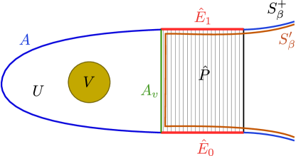
Figure 8. This figure crossed with $S^{1}$ illustrates the annulus case in Lemma 4.5. Crossed with $[0,1]$ and without the yellow disk, it illustrates the rectangle case.

Now replace $A$ with $A_{v}$ in $S^{+}_{\beta}$ to produce:

$$S_{\beta}^{\prime}=(S_{\beta}^{+}\setminus A)\cup A_{v}.$$

Push $S_{\beta}^{\prime}$ slightly further into $\mathcal{N}(\mathcal{B})$ so that it misses $A_{v}$.

This surface is isotopic to $S_{\beta}$ (through $U$), because the meridian $m_{\beta}$ meets $A_{v}$ and $A$ in a single arc. The isotopy does not change the intersection with the cores of the solid tori, but reduces the intersection with the 1-skeleton of ${\bf t}$. This is because, by Proposition 2.7, the annulus $A_{v}$, which is a component of $\partial_{v}\mathcal{N}(\mathcal{B})$, contains arcs of ${\bf t}^{(1)}$ which intersected $S^{+}_{\beta}$ but miss $S^{\prime}_{\beta}$. This contradicts the complexity-minimizing choice of $S_{\beta}$, also made possible by Proposition 2.7.

It remains to consider the case where each $\hat{E}_{i}$ is an essential rectangle, i.e. a nontrivial disk in $S_{\beta}^{+}$ which meets $\partial S_{\beta}^{+}$ along two arcs. Figure 8 again describes the situation, but one should interpret the diagram cross $[0,1]$ instead of $S^{1}$. Thus we see $\hat{E}_{1}$ and $\hat{E}_{2}$ as rectangles in $S^{+}_{\beta}$, and $\hat{P}$ as a cube, with its front and back faces (the diagram rectangle crossed with $\{0\}$ and $\{1\}$) lying in $\partial M_{\beta}$. The arcs labeled $A_{v}$ and $A$ represent rectangles lying in $\partial_{v}\mathcal{N}$ and $S^{+}_{\beta}$ respectively, and their union $A_{v}\cup A$ is a properly embedded annulus, whose boundary circles lie in the toroidal boundary $\partial M_{\beta}$.

Suppose it is not null-homotopic. Then, because $\mathring{M}$ is hyperbolic $A_{v}\cup A$ must be a boundary-parallel annulus. This means that each arc connecting its boundaries can be deformed rel endpoints to $\partial M_{\beta}$. Applying this to such an arc lying just in $A$, we obtain a boundary-compression of $S^{+}_{\beta}$, which is a contradiction.

Thus $A_{v}\cup A$ is null-homotopic so its boundary circles bound disks in $\partial M_{\beta}$ because $\partial M_{\beta}$ is incompressible. By irreducibility then the region between $A_{v}\cup A$ and these two disks is a ball, labeled $U$ in the figure.

Again by choosing $\hat{P}$ innermost we can assume that $U$ is a component of $X_{\beta}$. There is no component of $V_{\beta}$ in $U$ this time, since it is a ball, so it is in fact a component of $X$. This means that a disk $m_{\beta}$ constructed as a compression of the annulus $A_{v}\cup A$ is an actual monogon for $\mathcal{B}$ in $\mathring{M}$, and this is a contradiction to the incompressibility of $\mathcal{B}$.

This contradiction implies that $\mathcal{B}$ is orientable. ∎

4.6. Product structures are tame

We can now assemble the proof of the key fact that, for sufficiently long fillings, the foliation $\mathcal{I}|(\mathcal{F}_{\beta}\smallsetminus X_{\beta})$ comes from a product structure on $\mathcal{F}_{\beta}$.

Proposition 4.6.

For sufficiently long fillings, the foliation $\mathcal{I}|(\mathcal{F}_{\beta}\smallsetminus X_{\beta})$ can be extended to a foliation of all of $\mathcal{F}_{\beta}$. Consequently, $\mathcal{I}|(\mathcal{F}_{\beta}\smallsetminus X_{\beta})$ agrees with a product foliation $\mathcal{F}_{\beta}\cong S_{\beta}\times[0,1]$ (up to isotopy), and each component of $X_{\beta}$ is a subproduct of the associated product structure on $\mathcal{F}_{\beta}$.

Proof.

On each component $P$ of $\mathcal{F}_{\beta}\smallsetminus X_{\beta}$, the foliation $\mathcal{I}|(\mathcal{F}_{\beta}\smallsetminus X_{\beta})$ by intervals determines a product structure $E\times[0,1]$. Lemma 4.5 implies that $\mathcal{I}$ is orientable, and hence any leaf must intersect both components of $\partial\mathcal{F}_{\beta}$. In particular, $E\times\{0\}$ and $E\times\{1\}$ are components of $W_{i}$ on opposite sides of $\partial\mathcal{F}_{\beta}$. Furthermore, Lemma 4.4 implies that for all sufficiently long fillings $E\times\{0\}$ is not trivial. Therefore, Lemma 3.1 implies that the product structure of $\mathcal{F}_{\beta}$ can be isotoped so that it matches the product structure determined by the foliation $\mathcal{I}|(\mathcal{F}_{\beta}\smallsetminus X_{\beta})$. ∎

4.7. Fixed-fiber reduction and the completion of the proof.

We are now ready for the proofs of Theorems 1.5 and 1.4.

Proof of Theorem 1.5.

As in our setup so far (Section 4.2) we restrict attention to a single branched surface $\mathcal{B}$ and the associated fillings and fibers $\SS_{\mathcal{B}}$.

For $(S,\beta)\in\SS_{\mathcal{B}}$ sufficiently long we can apply Proposition 4.6, which tells us that the foliation $\mathcal{I}$ on $\mathcal{N}\cup V^{B}_{\beta}$ extends to $X_{\beta}$, giving a product foliation on $\mathcal{F}_{\beta}$ for which $X_{\beta}$ is a subproduct. The product structures on $\mathcal{F}_{\beta}$ and $\mathcal{T}_{\beta}$ define a specific mapping torus structure on $M_{\beta}$ and hence suspension flow $(\psi_{s})$ on $M_{\beta}$ (well-defined up to reparameterization). By construction of $\mathcal{I}$ on $V_{\beta}$, we see that $V_{\beta}$ is invariant by $(\psi_{s})$ and the $I$–fibers of $\mathcal{N}$ are arcs of flow lines.

In particular the cores of $V^{B}_{\beta}$ are already vertical with respect to this structure. Left to handle are the solid tori $V^{F}_{\beta}$, which may still be knotted in $\mathcal{F}_{\beta}$. To address this we need to establish additional uniformity which will allow us to invoke a theorem of Otal about unknottedness of short geodesics in Kleinian surface groups.

Let $\check{M}_{\beta}=\mathring{M}\cup V^{F}_{\beta}$ be the manifold obtained by filling $\mathring{M}$ along only the floating tori $V^{F}_{\beta}$, and note that $\check{M}_{\beta}=\mathcal{N}\cup X_{\beta}=M_{\beta}\smallsetminus\mathrm{int}(V^{B}_{\beta})$. Since $(\psi_{s})$ preserves $V^{B}_{\beta}$, it restricts to a flow on $\check{M}_{\beta}$.

Now we observe that for any surface $\mathring{S}$ fully carried by $\mathcal{B}$ – for example we can start with $(S,\beta_{0})$ in $M_{\beta_{0}}$ and remove intersections with $V^{B}_{\beta_{0}}$ – we can embed it in $\mathcal{N}$ in the standard way and view it as a surface in $\check{M}_{\beta}$ for a different value of $\beta$. We henceforth fix such a $\mathring{S}$ and allow $\beta$ to vary. Then $\mathring{S}$ is transverse to the flow $(\psi_{s})$ and in fact meets every flow line in forward and backward time; otherwise a flow half-line $\psi_{[s,\infty)}$ or $\psi_{(-\infty,s]}$ would miss $\mathcal{N}$ meaning that it was trapped in some component of $X_{\beta}$, which is impossible since $X_{\beta}$ is a product and the flow lines intersect it in compact arcs of the product foliation. Hence, there is a well-defined first return map $\phi\colon\mathring{S}\to\mathring{S}$ of $(\psi_{s})$ and $\check{M}_{\beta}$ is the mapping torus on $\phi$.

As in our previous constructions, we thicken $\mathring{S}$ to a product $\mathcal{T}_{\mathring{S}}$ and push it out along $I$–fibers of $\mathcal{N}$, so that $\partial_{h}\mathcal{T}_{\mathring{S}}$ contains $\partial_{h}\mathcal{N}$. The closure of the complement $\mathcal{F}_{\beta,\mathring{S}}$ is also a product, since $\mathring{S}$ is a fiber in $\check{M}_{\beta}$. Since the product structures on each of $\mathcal{T}_{\mathring{S}}$ and $\mathcal{F}_{\beta,\mathring{S}}$ are compatible with $(\psi_{s})$, it follows that $X_{\beta}$ is a subproduct of $\mathcal{F}_{\beta,\mathring{S}}$. Note that this product structure is the same up to isotopy as the product structure inherited from $\mathcal{F}_{\beta}$, since both are determined by the decomposition $\partial X_{\beta}=\partial_{h}X_{\beta}\cup\partial_{v}X_{\beta}$.

Consider the infinite cyclic cover $N_{\beta,\mathring{S}}$ of $\check{M}_{\beta}$ associated to $\mathring{S}$. Otal’s theorem [Ota95] implies that there is an $\ell>0$ depending only on $|\chi(\mathring{S})|$ so that if the cores of the solid tori $V_{\beta}^{F}$ have hyperbolic length less than $\ell$ then their lifts to $N_{\beta,\mathring{S}}\cong\mathring{S}\times\mathbb{R}$ are level. (We note that although Otal only explicitly treats the case where $\mathring{S}$ is closed, the general case is similar. Alternatively, the version needed here is explicitly stated by Bowditch [Bow11, Theorem 2.2.1] and also follows directly from a more general result of Souto [Sou08].) Henceforth, we consider only $\beta$ sufficiently long so that the cores of $V_{\beta}^{F}$ have length less than $\ell$, which is again possible by Thurston’s Dehn surgery theorem.

The product structure $N_{\beta,\mathring{S}}\cong\mathring{S}\times\mathbb{R}$ is obtained by gluing the $\mathbb{Z}$–indexed lifts of $\mathcal{T}_{\mathring{S}}$ and $\mathcal{F}_{\beta,\mathring{S}}$ together. Observe that all $V_{\beta}^{F}\subset X_{\beta}\subset\mathcal{F}_{\beta,\mathring{S}}$, and that $X_{\beta}$ is a subproduct of $\mathcal{F}_{\beta,\mathring{S}}$ by Proposition 4.6. By Lemma 3.3, working in one of the lifts of $\mathcal{F}_{\beta,\mathring{S}}$ to $N_{\beta,\mathring{S}}$ (which projects homeomorphically to $\check{M}_{\beta}$), the cores of $V_{\beta}^{F}$ are level in the product structure of $\mathcal{F}_{\beta,\mathring{S}}$, and further more the isotopy is supported in $X_{\beta}$. That is, after an isotopy, we may assume that the cores of $V_{\beta}^{F}$ are level with respect to $\mathring{S}$.

But the product structures on $X_{\beta}$ are isotopic, so we see that the cores of $V^{F}_{\beta}$ are level with respect to $\mathring{S}_{\beta}$, and hence $S_{\beta}$ as well. Since the cores of $V^{B}_{\beta}$ are already transverse, it follows that the cores of all filling solid tori $V_{\beta}$ are standard, and since $M$ is obtained from $M_{\beta}$ by drilling out these cores, we are done. ∎

We conclude this section by proving Theorem 1.4.

Proof of Theorem 1.4.

Fix $L>0$. If $\phi\in\Phi_{wp}(L)$, then $\mathrm{vol}(M_{\phi})\leq\frac{3}{2}\sqrt{2\pi}L$ by Theorem 2.4. By the Jørgensen–Thurston theorem [Thu78, Theorem 5.12.1], there is a finite collection $\mathcal{M}_{0}$ of hyperbolic $3$-manifolds of volume at most $V=\frac{3}{2}\sqrt{2\pi}L$ so that every hyperbolic $3$-manifold of volume at most $V$ is obtained from some manifold in $\mathcal{M}_{0}$ by hyperbolic Dehn filling.

Since the set $\mathcal{M}_{0}$ is finite, Theorem 1.5 gives that after excluding at most finitely many slopes per boundary component per manifold in $\mathcal{M}_{0}$, all other fillings of the manifolds in $\mathcal{M}_{0}$ have cores that are level or transverse.

For each $\mathring{M}\in\mathcal{M}_{0}$ choose a boundary component and consider the finitely many manifolds obtained by filling along the excluded slopes for that boundary. Let $\mathcal{M}_{1}$ be the collection of all such fillings over all members of $\mathcal{M}_{0}$. Since $\mathcal{M}_{1}$ is also finite, we may repeat the process of applying Theorem 1.5. Proceeding inductively, we terminate when no more fillings are needed to obtain elements of $\Phi_{wp}(L)$. Along the way we have accounted for all of the members of $\Phi_{wp}(L)$, showing that they come from our combined union of finite families by drilling along level or transverse curves. ∎

We end this section by describing an example of $1$–manifolds in a sequence of Dehn fillings on a compact manifold with hyperbolic interior, such that (a) each manifold fibers in infinitely many ways and (b) for all sufficiently long fillings, the $1$–manifold in each filling identified by the theorem is level with respect to one fiber and transverse with respect to another.

Example 1 (Level/transverse is relative).

Let $a$ and $b$ be homologous nonseparating curves that fill a closed surface $S$ of genus $g\geq 2$, and let $\phi_{n}=T_{a}^{n}\circ T_{b}^{-n}$ where $T_{c}$ is the Dehn twist about $c$. These mapping classes are pseudo-Anosov for $n\geq 1$ by Thurston’s construction [Thu88], and so the mapping tori $M_{n}=M_{\phi_{n}}$ are hyperbolic $3$–manifolds by Thurston’s hyperbolization theorem [Thu86a, Ota01].

We can view $M_{n}$ as obtained from a sequence of Dehn surgeries on $C=a\times\{\frac{2}{3}\}\cup b\times\{\frac{1}{3}\}$ in the mapping torus of the identity $M_{0}=S\times[0,1]/(x,1)\sim(x,0)\cong S\times\mathbb{S}^{1}$. By the Jørgensen–Thurston theorem [Thu78, Theorem 5.12.1], the sequence of hyperbolic manifolds $M_{n}=M_{f_{n}}$ limits to the cusped hyperbolic manifold $\mathring{M}=M_{n}\smallsetminus(a^{*}\cup b^{*})$ obtained by removing the geodesic representatives of $a$ and $b$ from $M_{n}$ for $n\gg 1$. This is the manifold obtained by drilling along (disjoint copies of) the level curves $a$ and $b$ of the fiber $S$ in any manifold of the sequence, and is homeomorphic to $M_{0}\setminus C$.

Now chose a different fiber $S_{n}$ of the manifold $M_{n}$ over the same fibered face as $S$ into which $a$ and $b$ cannot be homotoped (see §2.3). To see that it is possible to find such a fiber $S_{n}$, first observe that the Poincaré dual of $S$ lies in the subspace of $H^{1}(M)$ which vanishes on the homology class of $a$ (and $b$, since $a$ and $b$ are homologous). The linear subspace of $H^{1}(M)$ consisting of classes that vanish on this homology class has codimension $1$ since $\phi_{n}$ acts trivially on $H_{1}(S)$ (that is, $\phi_{n}$ is in the Torelli group), and hence any element of $H^{1}(S)$, in particular one that is nonzero on $a$, extends to an element of $H^{1}(M)$.

Since $a^{*}$ and $b^{*}$ become arbitrarily short as $n$ tends to infinity, these curves are necessarily a part of $\mathcal{C}$ from Theorem 1.5; in fact, their union is equal to $\mathcal{C}$. According to that theorem, $a$ and $b$ must be transverse in $S_{n}$, for $n$ sufficiently large. In fact, we see that $\mathring{M}$ is a fibered manifold with fibers $S_{n}$ punctured along $a\cup b$.

Therefore, for all $n$ sufficiently large, $a^{*}\cup b^{*}=\mathcal{C}$ in $M_{n}$ is level with respect to the fiber $S$ but transverse with respect to the fiber $S_{n}$.

5. Bounding Weil-Petersson translation length

In this section we prove the following theorem from the introduction.

Theorem 1.1. There exists $c>0$ so that if $\phi\colon S\to S$ is a pseudo-Anosov on a closed surface, $\alpha\subset S$ is a simple closed curve with $\tau_{\alpha}=\tau_{\alpha}(\phi)\geq 9$, and $k\in\mathbb{Z}$, then

$$\|T_{\alpha}^{k}\circ\phi\|_{wp}\leq\|\phi\|_{T}\sqrt{c|\chi(S)|}.$$

The bound on translation length in the theorem is obtained by producing an explicit $(T_{\alpha}^{k}\circ\phi)$–invariant path $\mathbb{R}\to\mathcal{T}(S)$ and bounding the WP-length of a fundamental domain for the action of $\langle T_{\alpha}^{k}\circ\phi\rangle$. The path is constructed as a leaf-wise conformal structure on the mapping torus of $T_{\alpha}^{k}\circ\phi$.

The remainder of this section is concerned with constructing the required structure and proving the bound on the Weil-Petersson translation length. We begin in Section 5.1 where we make precise what we mean by a suspension and leaf-wise conformal structure on a fibered $3$–manifold. This provides a more convenient framework for carrying out the construction. In Section 5.2 we describe the leaf-wise conformal structure coming from the singular-solv structure which is essentially the starting point for our construction. Since the singular-solv structure is constructed from the axis for a pseudo-Anosov with respect to the Teichmüller metric, this explains the appearance of $\|\phi\|_{T}$ in the bound we obtain.

Next, in Section 5.3 we describe how we will perform Dehn surgery on the manifold $M$, viewed as a suspension, so that the Dehn filled manifold is still a suspension, and the monodromy has been composed with a power of a Dehn twist. This is followed by Section 5.4, which contains two technical lemmas: one describes a particular solid torus in $M$ that is situated nicely with respect to the singular-solv structure; the second produces the explicit solid torus and leaf-wise conformal structure that we will use in our Dehn filling.

We assemble the ingredients in Section 5.5 and prove a more precise version of Theorem 1.1. In Section 5.6 we explain how to use this to show that $\Psi_{wp}(L)$ contains infinitely many conjugacy classes of pseudo-Anosov mapping classes on every closed, orientable surface of genus at least $2$, and finally in Section 5.7 we explain how to apply the theorem to produce examples in a much more general setting.

For the remainder of this section, we will take $\Sigma$ to be an arbitrary surface. The two cases of interest to us are when $\Sigma$ is a closed surfaces (in which case we often denote it by $S$) and when $\Sigma$ is an annulus (and we denote it $\mathbb{A}$).

5.1. Leaf-wise conformal structures

Suppose $\Sigma$ is a surface and $\pi\colon E\to B$ a $\Sigma$–bundle over a connected $1$–manifold $B$ which we view as either an interval in $\mathbb{R}$ or a circle $L\mathbb{S}^{1}=\mathbb{R}/L\mathbb{Z}$ of length $L>0$ (in particular, $\mathbb{R}$ locally acts on $B$ by translation). We consider local flows $\phi_{t}$ on $E$ such that for all $x\in E$ and $t\in\mathbb{R}$, $\pi(\phi_{t}(x))=\pi(x)+t$, as long as $\phi_{t}(x)$ is defined. If $E=\Sigma\times J$ for an interval $J\subseteq\mathbb{R}$ and $\pi$ the projection onto the second factor, then after changing the product structure we may assume that $\phi_{t}(x,s)=(x,s+t)$. For $s\in B$, we write $\Sigma_{s}=\pi^{-1}(s)$. Given $s,t\in B$, we can restrict $\phi_{t-s}$ to a homeomorphism

$$\phi_{t-s}\colon\Sigma_{s}\to\Sigma_{t}.$$

For fibrations $\pi\colon M\to L\mathbb{S}^{1}$ and $s,t\in L\mathbb{S}^{1}$, $t-s$ is only defined modulo $L\mathbb{Z}$. In this situation, we pass to the infinite cyclic cover of $M$ corresponding to the kernel of the homomorphism $\pi_{*}\colon\pi_{1}M\to\pi_{1}L\mathbb{S}^{1}\cong\mathbb{Z}$, and lift the flow and fibration over $L\mathbb{S}^{1}$ to a fibration over $\mathbb{R}$, to well-define $\phi_{t-s}$. Then we have $\Sigma_{0}=\Sigma_{L}$ in $M$ and $\phi=\phi_{L}\colon\Sigma_{0}\to\Sigma_{0}$ is the monodromy of the bundle. We refer to the bundle and flow $(\pi\colon M\to L\mathbb{S}^{1},(\phi_{t}))$ as a suspension (since $\phi_{t}$ is naturally the suspension flow of the monodromy $\phi$).

A leaf-wise conformal structure $\zeta$ on any $\Sigma$–bundle $E$ is a conformal structure on each surface $\Sigma_{s}$, making it into a Riemann surface $\Sigma_{s}^{\zeta}$, such that $\phi_{t-s}\colon\Sigma_{s}\to\Sigma_{t}$ is a quasi-conformal homeomorphism whenever it is defined. Let $\nu_{t,s}\in\mathbb{B}_{1}(\Sigma_{s}^{\zeta})\subset\mathbb{B}(\Sigma_{s}^{\zeta})$ denote the Beltrami differential of $\phi_{t-s}$.

If the path of Beltrami differentials $t\mapsto\nu_{t,s}\in\mathbb{B}_{1}(\Sigma_{s}^{\zeta})$ is piecewise smooth, we write

$$\mu_{s}^{\zeta}=\frac{d}{dt}\Big{|}_{t=s}\nu_{t,s}.$$

We call this the tangent field of the family. To justify this name, observe that the map $t\mapsto[\nu_{t,s}]\in\mathcal{T}(\Sigma_{s}^{\zeta})=\mathcal{T}(\Sigma)$ defines a path in the Teichmüller space and that $\mu_{t}^{\zeta}\in\mathbb{B}(\Sigma_{t}^{\zeta})$ represents the tangent vector at time $t$ to this path, for each $t\in J$.

Proposition 5.1.

Let $(\pi:M\to L\,\mathbb{S}^{1},(\phi_{t}))$ be a suspension with fibers $S_{t}=\pi^{-1}(t)$, let $\zeta$ be a leaf-wise conformal structure, and let $\mu_{t}^{\zeta}\in\mathbb{B}(S_{t}^{\zeta})$ be its tangent field. The mapping class $\phi=\phi_{L}\in\mathrm{Mod}(S_{0})$ has Weil-Petersson translation length $\|\phi\|_{wp}$ bounded by

$$\|\phi\|_{wp}\leq\int_{0}^{L}\left(\sqrt{\int_{S_{t}}|\mu^{\zeta}_{t}\sigma^{\zeta}_{t}|^{2}}\right)dt,$$

where $\sigma^{\zeta}_{t}$ is the hyperbolic metric uniformizing $S_{t}^{\zeta}$.

Proof of Proposition 5.1.

The translation length $\|\phi\|_{wp}$ is bounded from above by the length of the path

$$[0,L]\to\mathcal{T}(S_{0}),\ t\mapsto[\phi_{t}\colon S_{0}\to S_{t}^{\zeta}].$$

In formulas this means that

$$\|\phi\|_{wp}\leq\int_{0}^{L}\|\mu_{t}^{\zeta}\|_{wp}.$$

The desired bound follows now from Lemma 2.1. ∎

5.2. Singular solv structure

Suppose $\phi\colon S\to S$ is a pseudo-Anosov homeomorphism and $M=M_{\phi}$ is the mapping torus. The singular-solv metric on $M$ is a piecewise Riemannian metric that induces a Euclidean cone metric on the fibers of a fibration $\pi\colon M\to L\mathbb{S}^{1}$, where $L=\log(\lambda(\phi))=\|\phi\|_{T}$; see e.g. [CT07, McM00]. There is a natural unit speed flow $(\phi_{t})$ making $(\pi\colon M\to L\mathbb{S}^{1},(\phi_{t}))$ into a suspension so that:

1. The Euclidean cone metrics on the fibers defines a leafwise conformal structure $\zeta$,

2. the maps $\phi_{t-s}\colon S_{s}^{\zeta}\to S_{t}^{\zeta}$ are Teichmüller mappings for all $s,t$, with initial and terminal quadratic differentials $\varphi_{s}$ and $\varphi_{t}$, respectively,

3. for all $s,t$, the Beltrami differential of $\phi_{t-s}$ is given by $\nu_{t-s}=\tanh(t-s)\frac{\bar{\varphi}_{s}}{|\varphi_{s}|}$,

4. the tangent field is given by $\mu_{t}^{\zeta}=\frac{\bar{\varphi}_{t}}{|\varphi_{t}|}$, and

5. the vertical and horizontal foliations of $\varphi_{s}$ are the stable and unstable foliations for $\phi$, for all $s$.

Note that the tangent field $(\mu^{\zeta}_{t})$ to the singular-solv leaf-wise conformal structure $\zeta$ has $|\mu^{\zeta}_{t}|=1$, for all $t$. Therefore, applying Proposition 5.1, we obtain

$$\|\phi\|_{wp}\leq\int_{0}^{L}\left(\sqrt{\int_{S_{t}}|\mu^{\zeta}_{t}\sigma^{\zeta}_{t}|^{2}}\right)dt\leq\int_{0}^{L}\sqrt{\int_{S_{t}}(\sigma^{\zeta}_{t})^{2}}=L\sqrt{\mathrm{Area}(S)}=\|\phi\|_{T}\sqrt{\mathrm{Area}(S)},$$

as expected. To prove Theorem 1.1 we will perform an appropriate Dehn surgery on $M$ by drilling out the curve $\alpha$ on a fiber $S$, and replacing it with an appropriate solid torus and leaf-wise conformal structure. The goal of the next section is to describe the setup for such a surgery construction.

5.3. Dehn twists and Dehn filling

For any interval $J\subset\mathbb{R}$, the product

$$\mathbb{T}_{J}=\mathbb{A}\times J,$$

is a (not necessarily compact) solid torus. We denote the local flow in this special case by $\phi^{\mathbb{T}}_{t}(x,s)=(x,t+s)$ (defined for $s,t+s\in J$, as usual), and denote the projection onto the second factor by $\pi_{\mathbb{T}}:\mathbb{T}_{J}\to J$. In particular, we have $\pi_{\mathbb{T}}\phi^{\mathbb{T}}_{t}(x,s)=\pi_{\mathbb{T}}(x,s)+t=s+t$, where defined. As usual, we define $\mathbb{A}_{s}=\mathbb{A}\times\{s\}$ for all $s\in J$.

If we have a suspension $(\pi:M\to L\mathbb{S}^{1},(\phi_{t}))$, an embedding of a compact solid torus $\iota:\mathbb{T}_{J}\hookrightarrow M$, and an orientation preserving local isometry $\bar{\iota}\colon J\to L\mathbb{S}^{1}$, then we say that the suspension and solid torus are compatible (via $\iota$ and $\bar{\iota}$) if the following diagram commutes, whenever all maps are defined

Given a compatible suspension $(\pi\colon M\to L\mathbb{S}^{1},(\phi_{t}))$ and solid torus $\iota\colon\mathbb{T}_{J}\to M$ with $J=[a,b]$, let $M^{\prime}=M-\iota(\mathrm{int}(\mathbb{T}_{J}))$. For each $k$, the $\frac{1}{k}$–Dehn surgery on $\iota(\mathbb{T}_{J})$ in $M$ is obtained gluing $\mathbb{T}_{J}$ to $M^{\prime}$ via a homeomorphism $g_{k}\colon\partial\mathbb{T}_{J}\to\partial M^{\prime}=\iota(\partial\mathbb{T}_{J})$, given by

$$g_{k}(x)=\left\{\begin{array}[]{ll}\iota(x)&\mbox{for }x\in\mathbb{A}\times\{a\}\cup\partial\mathbb{A}\times J\\ \iota\circ t_{k}(x)&\mbox{for }x\in\mathbb{A}\times\{b\}.\end{array}\right.$$

where $t_{k}\colon\mathbb{A}\to\mathbb{A}$ is a homeomorphism representing the $k^{th}$ power of a Dehn twist in the core curve of $\mathbb{A}$. The resulting manifold $M_{k}=M^{\prime}\cup_{g_{k}}\mathbb{T}_{J}$ admits a flow $(\phi_{s})$ which locally agrees with the flow of the same name on $M^{\prime}\subset M$ and on $\mathbb{T}_{J}$ locally agrees with $(\phi_{s}^{\mathbb{T}})$, since the original solid torus was compatible. The monodromy is conjugate (by a power of $\phi$) to the composition $T_{\alpha}^{k}\circ\phi$, where $\alpha$ is a curve in $S_{0}$ in the isotopy class of the core of $\iota(\mathbb{T}_{J})$; see e.g. [Sta78, Har82, LM86].

5.4. Good solid tori

Throughout this section, we let $M=M_{\phi}$ for a pseudo-Anosov $\phi$. We will perform Dehn surgeries as described in the previous section in the presence of leaf-wise conformal structures on both $M$ and the filling solid tori $\mathbb{T}_{J}$. The leaf-wise conformal structure on $M$ will come from the singular-solv metric, and the solid torus which we will remove is described in Lemma 5.2 below. The leaf-wise conformal structure on $\mathbb{T}_{J}$ will be constructed by hand and will be such that the gluing maps restricted to the top and bottom $\mathbb{A}\times\partial J$ are conformal. This is described in Lemma 5.3. As the proofs of these are somewhat lengthy and technical, we defer their proofs to Section 6.

Recall that for any simple closed curve $\alpha\subset S$ the twisting coefficient of $\alpha$ for $\phi$, denoted $\tau_{\alpha}(\phi)$, is defined to be the distance in the subsurface projection to the annulus with core curve $\alpha$ of the stable and unstable laminations $\mathcal{L}_{+},\mathcal{L}_{-}$ for $\phi$:

$$\tau_{\alpha}(\phi)=d_{\alpha}(\mathcal{L}_{+},\mathcal{L}_{-}),$$

see [MM00] for details. As in Theorem 1.1 we now assume $\tau_{\alpha}=\tau_{\alpha}(\phi)\geq 9$.

The importance of this condition rests on a result of Rafi [Raf05] which provides a definite modulus Euclidean annulus (depending on $\tau_{\alpha}$) isometrically embedded in the Euclidean cone metric $\varphi_{t}$ defining the conformal structure $\zeta_{t}$ on $S_{t}$ for some $t$. Using $\phi_{t}$ to flow this backward and forward produces the required solid torus. Carrying out this construction carefully leads to the following, whose proof we defer to Section 6.6.

Lemma 5.2.

For some $h\geq\tfrac{1}{2}\operatorname{arccosh}(\tfrac{\tau_{\alpha}}{2}-3)$ and $J=[-h,h]$ there is an embedding $\iota\colon\mathbb{T}_{J}\to M$ compatible with the suspension $(\pi\colon M\to L\mathbb{S}^{1},(\phi_{t}))$ which is disjoint from the singularities. Furthermore, the induced leaf-wise conformal structure $\zeta$ on $\mathbb{T}_{J}$ agrees with the standard one on $\mathbb{A}_{-h}$, and there exists $\Psi\colon\mathbb{A}_{h}^{\zeta}\to\mathbb{A}_{-h}^{\zeta}$ conformal so $\Psi\circ\phi_{2h}^{\mathbb{T}}\colon\mathbb{A}_{-h}\to\mathbb{A}_{-h}$ is the $r^{th}$ power of a Dehn twist for some integer $r$.

To fill $M^{\prime}=M\setminus\iota(\mathrm{int}(\mathbb{T}_{J}))$ with $\mathbb{T}_{J}$ affecting an arbitrary Dehn twist in $\alpha$ as described in the previous subsection, we will need a different leaf-wise conformal structure on $\mathbb{A}_{J}$. To do this we essentially follow the same idea as in the proof of incompleteness of the Weil-Petersson metric by Wolpert [Wol75] and Chu [Chu76]. Specifically, we recall that the incompleteness comes from paths in Teichmüller space exiting every compact set in which a curve on the surface is “pinched” to have length tending to zero, but which nonetheless has finite WP-length. We apply this idea to first pinch $\alpha$ to be arbitrarily short along the first half of the interval $J$, then perform as much twisting as we like on a negligible sub-interval in the middle of $J$, and then “un-pinch”. By carrying out all the estimates using the complete (infinite area) hyperbolic structure on the interior of the annulus, we may apply the Scwartz-Pick Theorem to obtain upper bounds whenever the annulus is conformally embedded into a Riemann surface. The specific construction we use provides the following. It will be proven in Section 6.5.

Lemma 5.3.

Given $k\in\mathbb{Z}$, $h>0$, $\rho>1$, there exists a leaf-wise conformal structure $\eta_{k}$ on the solid torus $\mathbb{T}_{J}=\mathbb{A}\times J$ for $J=[-h,h]$ agreeing with the standard structure (of modulus $1$) on $\mathbb{A}_{-h}=\mathbb{A}$, with tangent field $(\mu_{s}^{\eta_{k}})$ identically zero in a neighborhood of $\partial\mathbb{A}\times J$, so that for all $s\in J$,

$$\int_{\mathbb{A}_{s}^{\eta_{k}}}|\mu_{s}^{\eta_{k}}\sigma_{s}^{\eta_{k}}|^{2}\leq\frac{8\rho\pi}{h^{2}},$$

where $\sigma_{s}^{\eta_{k}}$ is the complete hyperbolic metric on the interior of $\mathbb{A}_{s}$, and so the local flow $(\phi_{s}^{\mathbb{T}})$ restricted to the boundary circles are dilations. Moreover, there is a conformal map $T_{k}\colon\mathbb{A}_{h}^{\eta_{k}}\to\mathbb{A}_{-h}^{\eta_{k}}$ so that the composition $T_{k}\circ\phi_{2h}^{\mathbb{T}}\colon\mathbb{A}_{-h}^{\xi_{k}}\to\mathbb{A}_{-h}^{\xi_{k}}$ is the $k^{th}$ power of a Dehn twist in the core curve.

5.5. Proof of Theorem 1.1.

This theorem will follow easily from the following more precise version by setting $c=2\pi(1+\frac{6}{h^{2}})$.

Theorem 5.4.

Suppose $\phi\colon S\to S$ is a pseudo-Anosov on a closed surface, $\alpha\subset S$ is a simple closed curve with $\tau_{\alpha}\geq 9$, and $k\in\mathbb{Z}$. Then

$$\|T_{\alpha}^{k}\circ\phi\|_{wp}\leq\|\phi\|_{T}\sqrt{2\pi|\chi(S)|\left(1+\frac{6}{h^{2}}\right)}$$

for some $h\geq\tfrac{1}{2}\operatorname{arccosh}\left(\tfrac{\tau_{\alpha}}{2}-3\right)$.

Proof.

Suppose $\iota\colon\mathbb{T}_{J}\to M$ is the solid torus from Lemma 5.2 and $\Psi\colon\mathbb{A}_{h}\to\mathbb{A}_{-h}$ and $r$ as in Lemma 5.2. Fix $k\in\mathbb{Z}$, $\rho>1$, and let $\eta_{k}$ be the leaf-wise conformal structure on $\mathbb{T}_{J}$, and $T_{k}\colon\mathbb{A}_{h}\to\mathbb{A}_{-h}$ as in Lemma 6.4. We will prove the required bound for $\|T_{\alpha}^{k-r}\circ\phi\|_{wp}$, which will suffice since $k$ was arbitrary.

Let $M^{\prime}=M-\iota(\mathrm{int}(\mathbb{T}_{J}))$ and glue $\mathbb{T}_{J}$ to $M^{\prime}$ along their boundaries via the map

$$g_{k}\colon\partial\mathbb{T}_{J}\to\partial M^{\prime}=\iota(\partial\mathbb{T}_{J}),$$

given by

$$g_{k}(z,t)=\left\{\begin{array}[]{ll}\iota(z,t)&\mbox{for }(z,t)\in\mathbb{A}\times\{-h\}\cup\partial\mathbb{A}\times J\\ \iota\circ\Psi^{-1}\circ T_{k}(z,t)&\mbox{for }(z,t)\in\mathbb{A}\times\{h\}.\end{array}\right.$$

The resulting manifold $M_{k}=M^{\prime}\cup_{g_{k}}\mathbb{T}_{J}$ admits a flow $(\phi_{s})$ which locally agrees with the flow of the same name on $M^{\prime}\subset M$ and on $\mathbb{T}_{J}$ locally agrees with $(\phi_{s}^{\mathbb{T}})$, since the original solid torus was compatible. Let $\iota_{k}\colon\mathbb{T}_{J}\to M_{k}$ denote the compatible inclusion of the solid torus $\mathbb{T}_{J}$.

We claim that the leaf-wise conformal structures $\zeta$ on $M$ (restricted to $M^{\prime}$) and $\eta_{k}$ on $\mathbb{T}_{J}$ glue together to give a leaf-wise conformal structure $\zeta_{k}$ on $M_{k}$. Near $\mathbb{A}_{-h}$ in the fiber containing this annulus, $\mathbb{A}_{-h}^{\zeta}$ and $\mathbb{A}_{-h}^{\eta_{k}}$ are the standard structures, while near $\mathbb{A}_{h}$ in the fiber containing it, we note that the map $\Psi^{-1}\circ T_{k}\colon\mathbb{A}_{h}^{\eta_{k}}\to\mathbb{A}_{h}^{\zeta}$ is the composition of two conformal maps, hence is conformal. Near all other annuli, we have removed a locally isometrically embedded flat cylinder and glued in another one. Since $(\phi_{s}^{\mathbb{T}})$ is a dilation on the boundary for both $\zeta$ and $\eta_{k}$, the gluing maps of boundaries are in fact dilations, and the conformal structures can be explicitly glued together. Let $(\mu^{\zeta_{k}}_{s})$ denote the tangent field, which is given by $\mu^{\zeta}_{s}$ on $S_{t}\cap M^{\prime}$ and by $\mu^{\eta_{k}}_{s}$ on $S_{s}\cap\iota_{k}(\mathbb{T}_{J})$.

The monodromy of $M_{k}$ is given by $T_{\alpha}^{k-r}\circ\phi$. To see this, note that conjugating $\Psi^{-1}T_{k}$ by $\phi_{2h}^{\mathbb{T}}$ we get

$$(\phi_{2h}^{\mathbb{T}})^{-1}\Psi^{-1}T_{k}\phi_{2h}^{\mathbb{T}}=(\Psi\phi_{2h}^{\mathbb{T}})^{-1}(T_{k}\phi_{2h}^{\mathbb{T}})$$

which is the composition of the $k^{th}$ power of a Dehn twist and the inverse of the $r^{th}$ power of a Dehn twist, both in the core curve of the annulus. Thus we have changed the original monodromy by the $(k-r)^{th}$ power of a Dehn twist in the core curve of $\mathbb{A}_{h}$, which is the image of $\alpha$ by the flow. Hence the monodromy is conjugate (by a power of $\phi$) to $T_{\alpha}^{k-r}\phi$.

For any $s\in L\mathbb{S}^{1}$, set $S_{s}^{0}=S_{s}\cap M^{\prime}$. The closure of the complement of $S_{s}^{0}$ in $S_{s}$ is a disjoint union of annuli (slices of the product $\mathbb{T}_{J}=\mathbb{A}\times J$) which we denote

$$\overline{S_{s}-S_{s,0}}=\bigsqcup_{i=1}^{n(s)}\mathbb{A}_{s,i}.$$

The number of annuli $n(s)$ is bounded by $\frac{3}{2}|\chi(S)|$, which is the largest number of disjoint essential annuli on $S$ that are pairwise nonhomotopic.

Now we write the integral as a sum of integrals on the subsurfaces

$$\int_{S_{s}^{\zeta_{k}}}|\mu^{\zeta_{k}}_{s}\sigma^{\zeta_{k}}_{s}|^{2}=\int_{S_{s,0}^{\zeta_{k}}}|\mu^{\zeta_{k}}_{s}\sigma^{\zeta_{k}}_{s}|^{2}+\sum_{i=1}^{n(s)}\int_{\mathbb{A}_{s,i}^{\zeta_{k}}}|\mu^{\zeta_{k}}_{s}\sigma^{\zeta_{k}}_{s}|^{2}.$$

The flow in $M$ has unit Teichmüller speed, and so $|\mu^{\zeta}_{s}|=1$. Since $\mu^{\zeta_{k}}_{s}=\mu^{\zeta}_{s}$ on $S_{s,0}^{\zeta_{k}}=S_{s,0}^{\zeta}$, the first integral is bounded by the hyperbolic area (as it was with $M$ itself)

$$\int_{S_{s,0}^{\zeta_{k}}}|\mu^{\zeta_{k}}_{s}\sigma^{\zeta_{k}}_{s}|^{2}\leq\mathrm{Area}(S_{s,0}^{\zeta_{k}})\leq\mathrm{Area}(S_{s}^{\zeta_{k}})=2\pi|\chi(S)|.$$

Each annulus $\mathbb{A}_{s,i}$ is the $\iota_{k}$–image of $\mathbb{A}_{s(i)}$ where $\bar{\iota}_{k}(s(i))=s$, and $\iota_{k}$ induces a conformal map $\mathbb{A}_{s(i)}^{\eta_{k}}\to\mathbb{A}_{s,i}^{\zeta_{k}}$. By the Schwartz-Pick theorem, the hyperbolic metric $\sigma_{s}^{\zeta_{k}}$ on $S_{s}^{\zeta_{k}}$ restricted to $\mathbb{A}_{s}^{\zeta_{k}}$ is bounded above by the complete hyperbolic metric $\sigma_{s(i)}^{\eta_{k}}$ on $\mathbb{A}_{s(i)}^{\eta_{k}}\cong\mathbb{A}_{s,i}^{\zeta_{k}}$. Combining this with Lemma 6.4 implies that for each $i=1,\ldots,n(s)$,

$$\int_{\mathbb{A}_{s,i}^{\zeta_{k}}}|\mu^{\zeta_{k}}_{s}\sigma^{\zeta_{k}}_{s}|^{2}\leq\int_{\mathbb{A}_{s(i)}^{\zeta}}|\mu_{s(i)}^{\eta_{k}}\sigma_{s(i)}^{\eta_{k}}|^{2}\leq\frac{8\rho\pi}{h^{2}}.$$

Now, by Proposition 5.1 and since $n(s)\leq\frac{3}{2}|\chi(S)|$, we have

$$\|T_{\alpha}^{k-r}\circ\phi\|_{wp} \leq \displaystyle{\int_{0}^{L}\sqrt{\int_{S_{s}^{\zeta_{k}}}|\mu^{\zeta_{k}}_{s}\sigma^{\zeta_{k}}_{s}|^{2}}ds\leq\int_{0}^{L}\sqrt{2\pi|\chi(S)|+\sum_{i=1}^{n(s)}\frac{8\rho\pi}{h^{2}}}\,\,ds}$$

$$\leq \displaystyle{\|\phi\|_{T}\sqrt{2\pi|\chi(S)|+\frac{8\rho\pi}{h^{2}}\left(\frac{3}{2}|\chi(S)|\right)}}$$

Taking the limit as $\rho\to 1$, we obtain

$$\|T_{\alpha}^{k-r}\circ\phi\|_{wp} \leq \displaystyle{\|\phi\|_{T}\sqrt{2\pi|\chi(S)|\left(1+\frac{6}{h^{2}}\right)}}.$$

This completes the proof. ∎

We also record the following corollary of Theorem 1.1.

Corollary 5.5.

If $\|\phi\|_{T}\leq\frac{c^{\prime}}{|\chi(S)|}$ for some $c^{\prime}>0$, and if $\alpha$ is a curve with $\tau_{\alpha}(\phi)\geq 9$, then for all $k\in\mathbb{Z}$

$$\|T_{\alpha}^{k}\circ\phi\|_{wp}\leq\frac{c^{\prime}\sqrt{c}}{\sqrt{|\chi(S)|}}.$$

where $c$ is the constant from Theorem 1.1.∎

5.6. Examples in all genus.

From Corollary 5.5 we can prove Corollary 1.2 from the introduction, which we restate here, with an explicit bound on $L$.

Corollary 5.6.

For any $L\geq 124$ the set $\Phi_{wp}(L)$ contains infinitely many conjugacy classes of pseudo-Anosov mapping classes for every closed surface of genus $g\geq 2$.

Proof.

Consider the curves $\alpha,\alpha^{\prime},\beta$ on a genus two surface $S_{2}$ shown in Figure 9. Suppose $\phi_{2}\colon S_{2}\to S_{2}$ is the mapping class defined by $\phi_{2}=T_{\alpha^{\prime}}T_{\alpha}^{9}T_{\beta}^{-1}$. We can (explicitly) construct a square-tiled flat metric on $S$ so that $\beta$ is vertical and $\alpha,\alpha^{\prime}$ are horizontal, and so that $\phi_{2}$ is affine (c.f. Thurston’s construction [Thu88]). Specifically, this surface is built from a cylinder of height 9 and circumference 2 about $\alpha$ and height $1$ and circumference $2$ about $\alpha^{\prime}$ as shown in the middle of the figure. This can be done so that the derivative of $\phi_{2}$ is given by the matrix on the right of the figure.

Figure 9. Left: curves on a genus $2$ surface. Middle: square tiled surface built by isometrically identifying vertical sides by isometry in the obvious way and horizontal sides as indicated by the numbering. The tall rectangle has height $9$ and width 2, while the smaller one has height $1$ and width $2$. The horizotonal curves are $\alpha$ and $\alpha^{\prime}$ as labeled, and the vertical curve is $\beta$. Right: Derivative of the pseudo-Anosov $\phi_{2}$.

From this we compute that $\lambda(\phi_{2})=21+2\sqrt{110}$, and the eigenspaces of $D\phi_{2}$, which define the stable/unstable foliations for $\phi_{2}$, have slopes $\sqrt{110}-10\leq\frac{1}{2}$ and $-\sqrt{110}-10\leq-20$. From the description of the cylinder about $\alpha$, we see that $\tau_{\alpha}\geq 11$.

Now let $M$ be the mapping torus of $\phi_{2}$. Since $\alpha$ and $\beta$ intersect twice, as was shown in [ALM16, Lemma 3.8-3.9], there is a genus $2$ surface $S^{\prime}\subset M$ which contains $\alpha$ and is transverse to the suspension flow of $\phi_{2}$. Thus $S^{\prime}$ represents a class $[S^{\prime}]$ in the closure of the cone $\mathcal{C}=\mathbb{R}_{+}F$ on the fibered face $F$ of the Thurston norm ball ${\bf B}$ containing the class $[S]$ of $S$. In fact, it was also shown in [ALM16] that $[S]$ and $[S^{\prime}]$ are linearly independent. It follows that for all $g\geq 3$, the class $(g-2)[S]+[S^{\prime}]$ is represented by a surface $S_{g}$ which is a fiber in a fibration of $M$ over $S^{1}$ and contains $\alpha$. By linearity of the Thurston norm $\mathfrak{n}$, $-\chi(S_{g})=\mathfrak{n}(S_{g})=2g-2$, and since $[S_{g}]$ is primitive, $S_{g}$ is connected of genus $g$; see Theorem 2.5. Moreover, since both $S$ and $S^{\prime}$ contain $\alpha$, we can realize $S_{g}$ so that it also contains $\alpha$.

Let $\phi_{g}\colon S_{g}\to S_{g}$ denote the monodromy. Recall from Theorem 2.6 that $\mathfrak{h}\colon\mathcal{C}\to\mathbb{R}_{+}$, which extends $\|\cdot\|_{T}$, is convex and homogeneous of degree $-1$ and thus

$$\|\phi_{3}\|_{T}=\mathfrak{h}([S_{3}])\leq\mathfrak{h}([S_{2}])=\|\phi_{2}\|;$$

see [ALM16, Lemma 3.11]. Applying convexity again we have

$$|\chi(S_{g})|\|\phi_{g}\|_{T}\leq 4\log(\lambda(\phi_{2}))=4\log(21+2\sqrt{110})\leq 14.95.$$

The twisting numbers $\tau_{\alpha}(\phi_{g})$ and $\tau_{\alpha}(\phi_{2})$ are equal: this is because these are twisting numbers for the monodromy maps of fibers $[S]$ and $[S_{g}]$ in the same fibered face of the Thurston norm ball. As observed in [MT17], the universal covers of $S$ and $S_{g}$ can both be identified with the leaf space of the suspension flow in the universal cover of $M$, the stable/unstable laminations of $\phi_{2}$ and $\phi_{g}$ have identical lifts in this cover, and $\tau_{\alpha}$ is computed using this data in the annular quotient associated to the conjugacy class $[\alpha]$ in $\pi_{1}(M)$.

In particular $\tau_{\alpha}(\phi_{g})=\tau_{\alpha}(\phi_{2})\geq 11$. Therefore, by Corollary 5.5, we have

$$\|T_{\alpha}^{k}\circ\phi_{g}\|_{wp}\leq\sqrt{c}\frac{14.95}{\sqrt{|\chi(S_{g})|}}\leq\frac{124}{\sqrt{|\chi(S_{g})|}},$$

where we have used $c=2\pi\left(1+\frac{6}{h^{2}}\right)$ with $h=\tfrac{1}{2}\operatorname{arccosh}\left(\tfrac{11}{2}-3\right)$. It follows that $\Phi_{wp}(L)$ contains infinitely many pseudo-Anosov mapping classes on every surface of genus $g\geq 2$ for $L\geq 124$. ∎

5.7. Generalities

This construction is much more robust, as the following corollary shows. Given a closed curve $\alpha$ in $M$, there is a subspace $V_{\alpha}\subset H^{1}(M)$ consisting of cohomology classes that evaluate to zero on $\alpha$.

Corollary 5.7.

Suppose $M$ is a closed fibered $3$–manifold with pseudo-Anosov monodromy $\phi\colon S\to S$, and suppose that $\alpha$ is a curve in $S$. Then there is a constant $c_{0}>0$ and an $\mathbb{R}_{+}$–invariant neighborhood $U$ of $[S]\in H^{1}(M)$ with the following property. If $S^{\prime}\subset M$ is another fiber of $M$ with $[S^{\prime}]\in U\cap V_{\alpha}$, then $\alpha$ is isotopic into $S^{\prime}$, and for all $k\in\mathbb{Z}$, the monodromy $\phi^{\prime}\colon S^{\prime}\to S^{\prime}$ satisfies

$$\|T_{\alpha}^{k}\circ\phi^{\prime}\|_{wp}\leq\frac{c_{0}}{\sqrt{|\chi(S^{\prime})|}}.$$

Observe that this corollary does not require any assumption on the twisting coefficient of $\alpha$, though one loses explicit control on $c_{0}$ because of this.

Proof.

Since $S$ is a fiber we can represent $[S]\in H_{2}(M)\cong H^{1}(M)$ as a closed 1-form $\omega$ which is nowhere zero. Fixing a Riemannian metric on $M$, for each $\epsilon$ let $U_{\epsilon}$ denote a neighborhood of $[S]$ with the property that every element in $U_{\epsilon}$ is represented by a closed nowhere-zero $1$-form $\omega^{\prime}$ with $|\omega^{\prime}-\omega|<\epsilon$. The primitive integral classes in $\mathbb{R}_{+}U_{\epsilon}$ are precisely the classes in $\mathbb{R}_{+}U_{\epsilon}$ dual to fibers of a fibration.

We would like to say that there is a regular neighborhood $N$ of $\alpha$ and an $\epsilon>0$ such that when $S^{\prime}$ is a fiber with $[S^{\prime}]\in\mathbb{R}^{+}U_{\epsilon}\cap V_{\alpha}$ then after an isotopy both $S$ and $S^{\prime}$ meet $N$ in an annulus containing $\alpha$.

First choose a regular neighborhood $W$ which can be written in the form $A\times(-b,b)$ where $A_{0}=A\times\{0\}$ is a regular neighborhood of $\alpha$ in $S$ and $\omega|_{W}=dt$, where $t$ is the coordinate for $(-b,b)$. If $\omega^{\prime}$ is the 1-form representing $[S^{\prime}]$ then, since $[S^{\prime}]\in V_{\alpha}$, we have $\int_{\alpha}\omega^{\prime}=0$ so $\omega^{\prime}$ is exact in $W$. For suitably small $\epsilon$ we can write $\omega^{\prime}=dh$ on $W$.

Thus for small $\epsilon$ the level sets of $h$ are surfaces transverse to the $t$ direction. It follows that there is a smaller regular neighborhood $N$ of $\alpha$ so that for each $\omega^{\prime}$ representing a point in $U_{\epsilon}$ there is a compactly supported isotopy in $W$ (moving along vertical lines) which takes $\omega^{\prime}$ to $dt$ in $N$. The integral manifold of (the isotope of) $\ker\omega^{\prime}$ passing through $\alpha$ contains the annulus $A_{0}\cap N$, and after another isotopy any other intersections of it with $N$ can be pushed off. This gives the desired fiber $S^{\prime}$.

Now in $H_{1}(\partial N)$ we have a basis $\mu,\lambda$ where $\mu$ is the boundary of a meridian disk and $\lambda$ is represented by a component of $\partial(A_{0}\cap N)$. Let $\mathring{M}=M\smallsetminus N$. For $j\in\mathbb{Z}$, the Dehn filling of $\mathring{M}$ associated to $\mu+j\lambda$ gives a manifold $M_{j}$ that can be simultaneously described as the mapping torus of $T^{j}_{\alpha}\phi$, and as the mapping torus of ${T^{\prime}_{\alpha}}^{j}\phi^{\prime}$, where $\phi$ is the monodromy of the fibering of $S$, $\phi^{\prime}$ is the monodromy of the fibering of $S^{\prime}$, and $T_{\alpha}$ and $T^{\prime}_{\alpha}$ are the Dehn twist of $\alpha$ in $A_{0}\cap N$, considered as a homeomorphism of $S$ and $S^{\prime}$ respectively.

We want to relate homology classes in $M$ to those in $M_{j}$. Note that the inclusion map $H_{2}(\mathring{M})\to H_{2}(M)$ is injective (since $\partial\mathring{M}=\partial N$ has one component), and that its image is exactly $V_{\alpha}$ (this is an exercise in Poincaré duality). Thus we can invert it on $V_{\alpha}$ and compose with the inclusion $H_{2}(\mathring{M})\to H_{2}(M_{j})$ to obtain a linear map $V_{\alpha}\to H_{2}(M_{j})$. Let $\mathcal{F}_{j}$ denote the fibered face of the Thurston norm ball in $H_{2}(M_{j})$ containing the image $[S_{j}]$ of $[S]$. Then $\mathbb{R}_{+}\mathcal{F}_{j}$ is open, and we may choose $\epsilon$ sufficiently small that it contains the closure of the image of $\mathbb{R}_{+}U_{\epsilon}\cap V$, which we denote $K_{j}$. Let $[S^{\prime}_{j}]$ denote the image of $[S^{\prime}]$ in $H_{2}(M_{j})$.

Now let $U=\mathbb{R}^{+}U_{\epsilon}$, and choose $j>0$ so that $T^{j}_{\alpha}\phi$ is pseudo-Anosov and $\tau_{\alpha}(T^{j}_{\alpha}\phi)\geq 9$.

For any $S^{\prime}$ such that $[S^{\prime}]\in U\cap V_{\alpha}$, as observed above in the proof of Corollary 5.5, the twisting numbers $\tau_{\alpha}(T^{j}_{\alpha}\phi)$ and $\tau_{\alpha}({T^{\prime}_{\alpha}}^{j}\phi^{\prime})$ are equal since $[S_{j}]$ and $[S^{\prime}_{j}]$ are in the same fibered face $\mathcal{F}_{j}$.

In particular $\tau_{\alpha}({T^{\prime}_{\alpha}}^{j}\phi^{\prime})\geq 9$ and we can therefore apply Theorem 1.1 to ${T^{\prime}_{\alpha}}^{j}\phi^{\prime}$, obtaining

$$\|{T^{\prime}_{\alpha}}^{k}\circ\phi^{\prime}\|_{wp} =\|{T^{\prime}_{\alpha}}^{k-j}\circ{T^{\prime}_{\alpha}}^{j}\phi^{\prime}\|_{wp}$$

$$\leq\|{T^{\prime}_{\alpha}}^{j}\phi^{\prime}\|_{T}\sqrt{c|\chi(S^{\prime})|}.$$

To complete the argument we need to obtain a bound on $\|{T^{\prime}_{\alpha}}^{j}\phi^{\prime}\|_{T}$. As described in Section 2.3, by Theorem 2.6 there is a $c_{j}\geq 1$ depending only on $K_{j}$ such that if $S^{\prime\prime}$ is a fiber of $M_{j}$ such that $[S^{\prime\prime}]\in K_{j}$ with monodromy $\phi_{S^{\prime\prime}}$ then $|\chi(S^{\prime\prime})|\|\phi_{S^{\prime\prime}}\|_{T}\leq c_{j}$. We conclude that

$$\|{T^{\prime}_{\alpha}}^{k}\circ\phi^{\prime}\|_{wp}\leq\frac{c_{j}\sqrt{c}}{\sqrt{|\chi(S^{\prime})|}},$$

as required. ∎

6. Constructions and estimates

In this section, we will describe constructions of some specific leaf-wise conformal structures and estimates for the Weil-Petersson norm of their tangent fields. We begin with some generalities on reparameterizing and gluing leaf-wise conformal structures. Next we set up some notation for annuli and carry out some computations of hyperbolic area, before turning to the construction of the required leaf-wise conformal structures on solid tori from Lemma 5.3 necessary for our main construction. We end this section with the construction of the solid torus from Lemma 5.2 we remove from the original manifold $M$.

6.1. Reparameterizing and gluing

Given a piecewise differentiable, monotone, surjective map $g\colon I\to J$, we define $G\colon\Sigma\times I\to\Sigma\times J$ by $G(x,t)=(x,g(t))$. If $\zeta$ is a leaf-wise conformal structure on $\Sigma\times J$, then it pulls back via $G$ to one on $\Sigma\times I$ denoted $G^{*}\zeta$, so that $\Sigma_{s}^{G^{*}\zeta}=\Sigma_{g(s)}^{\zeta}$ as Riemann surface structures on $\Sigma$. For any $s\in I$, the resulting path of Beltrami differentials in $\mathbb{B}_{1}(\Sigma_{s}^{G^{*}\zeta})=\mathbb{B}_{1}(\Sigma_{g(s)}^{\zeta})$ is just the composition $t\mapsto\nu_{g(t),g(s)}$, and consequently the tangent field is given by

$$\mu_{s}^{G^{*}\zeta}=g^{\prime}(s)\mu_{g(s)}^{\zeta}.$$

Suppose that $\zeta_{1}$ and $\zeta_{2}$ are leaf-wise conformal structures on $\Sigma\times J_{1}$ and $\Sigma\times J_{2}$, respectively, such that $J_{1}\cap J_{2}=\{s\}$ and there is a conformal map $g\colon\Sigma_{s}^{\zeta_{1}}\to\Sigma_{s}^{\zeta_{2}}$. Then we can glue together the leaf-wise conformal structures to a single leaf-wise conformal structure $\zeta$ on $\Sigma\times J_{1}\cup J_{2}$ using the conformal map $g$. More precisely, we define the leaf-wise conformal structure on $\Sigma\times J_{1}$ to be $\zeta_{1}$ and on $\Sigma\times J_{2}$ to be $g^{*}\zeta_{2}$. The path in Teichmüller space $J\to\mathcal{T}(\Sigma)$ is the concatenation of the path $J_{1}\to\mathcal{T}(\Sigma)$ with $J_{2}\to\mathcal{T}(\Sigma)$ after adjusting the marking of the latter by the conformal map $g$.

6.2. Annuli and solid tori

As above, we let $L\mathbb{S}^{1}=\mathbb{R}/L\mathbb{Z}$ denote a circle of length $L>0$. Any annular Riemann surfaces with finite modulus can be uniformized by Euclidean metrics of the form $L\mathbb{S}^{1}\times J$, where $J\subset\mathbb{R}$ is an interval; the conformal modulus is $|J|/L$. Equivalently, this surface is the quotient

$$L\mathbb{S}^{1}\times J=\{z=x+iy\in\mathbb{C}\mid y\in J\}/\langle z\mapsto z+L\rangle.$$

Note that $L\mathbb{S}^{1}\times J$ is conformally equivalent to $rL\mathbb{S}^{1}\times rJ$, for any $r>0$, and we will write $m\mathbb{A}$ for any annular Riemann surface with conformal modulus $m$. For $m=1$, we just write $1\mathbb{A}=\mathbb{A}$, though we also allow $\mathbb{A}$ to denote a topological annulus.

The middle sub-annulus of the annulus $2m\mathbb{A}$ of modulus $2m$ is the sub-annulus of modulus $m$ invariant under the full conformal automorphism group. More precisely, it is given by

$$\mathbb{S}^{1}\times\left[-\tfrac{m}{2},\tfrac{m}{2}\right]\subset\mathbb{S}^{1}\times[-m,m].$$

Although the middle sub-annulus encompasses half the Euclidean area, it’s hyperbolic area is inversely proportional to the modulus, as the next lemma shows.

Lemma 6.1.

Suppose $m\mathbb{A}\subset 2m\mathbb{A}$ is the middle sub-annulus and $\sigma$ is the complete hyperbolic metric on the interior of $2m\mathbb{A}$. Then

$$\int_{m\mathbb{A}}\sigma^{2}=\frac{\pi}{m}.$$

Proof.

We view the annulus $2m\mathbb{A}$ as the quotient of

$$H_{m}=\{x+iy\in\mathbb{C}\mid|y|\leq m\},$$

by the action of $\langle z\mapsto z+1\rangle$. A fundamental domain for the middle sub-annulus is

$$D_{\tfrac{m}{2}}=\{x+iy\mid 0\leq x\leq 1,\,-\tfrac{m}{2}\leq y\leq\tfrac{m}{2}\}\subset H_{\tfrac{m}{2}}\subset H_{m}.$$

To find the hyperbolic metric on the interior of $H_{m}$, map it to the upper half-plane with the conformal map $z\mapsto ie^{\frac{\pi z}{2m}}$. The pull-back to $H_{m}$ of the hyperbolic metric $\frac{|dz|}{Im(z)}$ in the upper-half plane is

$$\tilde{\sigma}=\frac{\pi}{2m\cos(\tfrac{\pi y}{2m})}|dz|=\frac{\pi}{2m}\sec(\tfrac{\pi y}{2m})|dz|.$$

Therefore, integrating this over $D_{\tfrac{m}{2}}$ provides the required computation:

$$\int_{\mathbb{A}_{m}}\!\!\!\sigma^{2}=\!\!\int_{D_{\tfrac{m}{2}}}\!\!\!\tilde{\sigma}^{2}=\!\!\int_{D_{\tfrac{m}{2}}}\!\!\!\!\tfrac{\pi^{2}}{4m^{2}}\sec^{2}(\tfrac{\pi y}{2m})|dz|^{2}\!\!=\!\tfrac{\pi^{2}}{4m^{2}}\!\!\int_{0}^{1}\!\!\int_{-m/2}^{m/2}\!\!\!\!\sec^{2}(\tfrac{\pi y}{2m})\,dy\,dx\!=\!\frac{\pi}{m}.$$

∎

In the next three subsections, we carry out the explicit construction of a leaf-wise conformal structure on solid tori and estimates on the Weil-Petersson norm of the associated tangent fields. This really divides into three parts: pinching, twisting, and then combining the two. Some care is necessary with the parameterizations involved since, when using these solid tori in Dehn filling, a fiber will typically meet the solid torus in many copies of the annulus.

6.3. Pinching construction/estimates

Here we explicitly describe the leaf-wise conformal structure on a solid torus that “pinches the core curve,” and estimate the Weil-Petersson norm of its tangent field. Specifically, for $h>0$ and solid torus $\mathbb{A}\times[0,h)$ we construct a leaf-wise conformal structure that has modulus $1$ on $\mathbb{A}_{0}$, modulus of $\mathbb{A}_{t}$ tending to infinity as $t\to h$, and so that the Weil-Petersson norm of the tangent field is bounded by $\frac{\sqrt{8\pi}}{h}$ for every $t$. The desired structure will be obtained from the one in the following proposition by an appropriate reparameterization.

Proposition 6.2.

There exists a leaf-wise conformal structure $\zeta$ on $\mathbb{A}\times[1,\infty)$ such that

1. $\mathbb{A}^{\zeta}_{t}$ is isomorphic to $t\mathbb{A}$.

2. The associated flow $\phi_{s}:\mathbb{A}^{\zeta}_{t}\to\mathbb{A}^{\zeta}_{t+s}$ is conformal in neighborhoods of the boundaries, and is a dilation on the boundaries.

3. The tangent field $\mu^{\zeta}_{t}$ satisfies $|\mu^{\zeta}_{t}|=1/t$ in the middle annulus of $\mathbb{A}^{\zeta}_{t}$, and is identically $0$ outside it.

In particular, we have

(2) $$\int_{\mathbb{A}_{t}^{\zeta}}|\mu_{t}^{\zeta}\sigma_{t}^{\zeta}|^{2}=\frac{2\pi}{t^{3}},$$

and therefore

(3) $$\int_{1}^{\infty}\sqrt{\int_{\mathbb{A}_{t}^{\zeta}}|\mu_{t}^{\zeta}\sigma_{t}^{\zeta}|^{2}}\,dt=\sqrt{8\pi}.$$

Note that this construction gives a path of finite Weil-Petersson length that diverges in Teichmüller space, by embedding $\mathbb{A}_{1}$ into some Riemann surface and using this family to deform. This recovers the result, due to Wolpert [Wol75] and Chu [Chu76], that the WP metric is incomplete.

Proof.

To begin, we define a $1$–parameter family of quasi-conformal maps $(\tilde{f}_{t}\colon\mathbb{C}\to\mathbb{C})_{t\geq 1}$, so that, defining

$$H_{s}=\{x+iy\in\mathbb{C}\mid|y|\leq s\},$$

• $\tilde{f}_{t}$ is the identity on the real coordinate $x$,

• $\tilde{f}_{t}$ takes $H_{1/t}$ to $H_{t}$, dilating the $y$ coordinate by $t^{2}$,

• $\tilde{f}_{t}$ takes $H_{1}$ to $H_{2t-1}$ and $H_{2}$ to $H_{2t}$.

Explicitly, $\tilde{f}_{t}$ is defined by

$$\tilde{f}_{t}(x+iy)=\left\{\begin{array}[]{ll}x+i(t^{2}y)&\mbox{ for }0\leq y\leq 1/t,\\ \\ x+i(2t-\frac{1}{y})&\mbox{ for }1/t\leq y\leq 1,\\ \\ x+i(y+2(t-1))&\mbox{ for }1\leq y,\\ \end{array}\right.$$

and extend over $x+iy\in\mathbb{C}$ with $y<0$ by reflection.

Now since horizontal translations in $\mathbb{C}$ commute with $\tilde{f}_{t}$ and preserve $H_{s}$ for all $s,t$, the map $\tilde{f}_{t}$ descends to a map

$$f_{t}\colon\mathbb{A}=H_{2}/\langle z\mapsto z+4\rangle\to H_{2t}/\langle z\mapsto z+4\rangle=t\mathbb{A}.$$

These maps define a leaf-wise conformal structure $\zeta$ on the (noncompact) solid torus $\mathbb{A}\times[1,\infty)$ so that $\mathbb{A}_{t}^{\zeta}=t\mathbb{A}$ and $\phi^{\mathbb{T}}_{t-1}=f_{t}\colon\mathbb{A}_{1}^{\zeta}\to\mathbb{A}_{t}^{\zeta}$.

Parts (a) and (b) of the proposition follow immediately from the definition. For part (c) and the two integral equalities, we need to compute the tangent field $\mu^{\zeta}_{t}$.

For any fixed $t\geq 1$, $s\geq 0$, consider the maps $\tilde{f}_{t,t+s}=\tilde{f}_{t+s}\circ\tilde{f}_{t}^{-1}\colon\mathbb{C}\to\mathbb{C}$. If $y\geq t$, then

$$\tilde{f}_{t,t+s}(x+iy)=x+i(y+2s),$$

while if $-y\geq t$, then $\tilde{f}_{t,t+s}(x+iy)=x+i(y-2s)$.

On the other hand, if $0\leq|y|<t$, then for sufficiently small $s>0$, we have

$$\tilde{f}_{t,t+s}(x+iy)=\tilde{f}_{t+s}(x+i(y/t^{2}))=x+i\left(\frac{(t+s)^{2}}{t^{2}}y\right).$$

In particular, if $\tilde{\nu}_{t,t+s}$ is the Beltrami coefficient of $\tilde{f}_{t,t+s}$, then for each $t$, its derivative with respect to $s$ at $s=0$ is

$$\tilde{\mu}_{t}(x+iy)=\left\{\begin{array}[]{cl}0&\mbox{ for }|y|\geq t\\ -\frac{1}{t}&\mbox{ for }|y|<t\end{array}\right.$$

The tangent field $\mu_{t}^{\zeta}$ is the descent of $\tilde{\mu}_{t}$, so we see that part (c) holds. Integrating this over $\mathbb{A}_{t}^{\zeta}=t\mathbb{A}$, we have

$$\int_{\mathbb{A}_{t}^{\zeta}}|\mu_{t}^{\zeta}\sigma_{t}^{\zeta}|^{2}=\frac{1}{t^{2}}\int_{\tfrac{t}{2}\mathbb{A}}\sigma_{t}^{2}=\frac{1}{t^{2}}\frac{\pi}{t/2}=\frac{2\pi}{t^{3}},$$

where the second equality is by Lemma 6.1. This proves equality (2). An easy computation proves (3). ∎

We can reparameterize the family of Proposition 6.2 by the moral equivalent of Weil-Petersson arclength to obtain the following:

Corollary 6.3.

For any $h>0$, there exists a differentiable homeomorphism $g\colon[0,h)\to[1,\infty)$ so that if $G\colon\mathbb{A}\times[0,h)\to\mathbb{A}\times[1,\infty)$ is the induced map of products and $\xi=G^{*}\zeta$ the pull-back of the leaf-wise conformal structure $\zeta$ on $\mathbb{A}\times[1,\infty)$ as above, with tangent field $\mu_{s}^{\xi}$, then

$$\int_{\mathbb{A}_{s}^{\xi}}|\mu^{\xi}_{s}\sigma^{\xi}_{s}|^{2}=\frac{8\pi}{h^{2}}.$$

Proof.

Set

$$s(t)=\int_{1}^{t}\sqrt{\int_{\mathbb{A}_{u}^{\zeta}}|\mu_{u}^{\zeta}\sigma_{u}^{\zeta}|^{2}}\,du=\int_{1}^{t}\frac{\sqrt{2\pi}}{u^{3/2}}\,du=\sqrt{8\pi}(1-t^{-1/2}).$$

Let $t(s)$ be the inverse (given by $t(s)=\frac{8\pi}{(\sqrt{8\pi}-s)^{2}}$) which satisfies

$$t^{\prime}(s)=\frac{1}{s^{\prime}(t(s))}=\frac{t(s)^{3/2}}{\sqrt{2\pi}}.$$

For any $h>0$, set $g(s)=t(\sqrt{8\pi}s/h)$, and observe that $g([0,h))=[1,\infty)$ with

$$g^{\prime}(s)=\frac{\sqrt{8\pi}}{h}t^{\prime}(\sqrt{8\pi}s/h)=\frac{\sqrt{8\pi}}{h}\frac{t(\sqrt{8\pi}s/h)^{3/2}}{\sqrt{2\pi}}=\frac{2g(s)^{3/2}}{h}.$$

Therefore, setting $G\colon\mathbb{A}\times[0,h)\to\mathbb{A}\times[1,\infty)$ the reparameterization and $\xi=G^{*}\zeta$, we have

$$\int_{\mathbb{A}_{s}^{\xi}}|\mu_{s}^{\xi}\sigma_{s}^{\xi}|^{2} = \int_{\mathbb{A}_{g(s)}^{\zeta}}|g^{\prime}(s)\mu_{g(s)}^{\zeta}\sigma_{g(s)}^{\zeta}|^{2}$$

$$= \frac{4g(s)^{3}}{h^{2}}\int_{\mathbb{A}_{g(s)}^{\zeta}}|\mu_{g(s)}^{\zeta}\sigma_{g(s)}^{\zeta}|^{2}$$

$$= \frac{4g(s)^{3}}{h^{2}}\frac{2\pi}{g(s)^{3}}=\frac{8\pi}{h^{2}},$$

as required. ∎

6.4. Twisting construction/estimates.

Here we use an affine twist in the middle sub-annulus and a simple construction to produce a solid torus $\mathbb{A}\times[-\epsilon,\epsilon]$ with arbitrarily small $\epsilon$, and leaf-wise conformal structure for which the Weil-Petersson norm of the tangent field is also arbitrarily small, and which affects the $k^{th}$ power of the Dehn twist in the core curve. The trade-off is that the moduli of $\mathbb{A}_{t}$ are required to be large.

Lemma 6.4.

Given $k\in\mathbb{Z}$, $\epsilon>0$, and $\delta>0$ there exists $m_{k}>0$ so that for any $m>m_{k}$, there exists a leaf-wise conformal structure $\xi_{k}$ on $\mathbb{T}_{\epsilon}=\mathbb{A}\times[-\epsilon,\epsilon]$ with associated tangent field $(\mu^{\xi_{k}}_{s})$, which is identically zero outside the middle sub-annulus for each $\mathbb{A}_{s}^{\xi_{k}}$, so that for all $s\in[-\epsilon,\epsilon]$, $\mathbb{A}_{s}^{\xi_{k}}$ has modulus $2m$,

$$\int_{\mathbb{A}_{s}^{\xi_{k}}}|\mu^{\xi_{k}}_{s}\sigma_{s}^{\xi_{k}}|^{2}<\delta,$$

and the local flow $(\phi_{s}^{\mathbb{T}})$ restricted to the boundary circles are dilations.

Moreover, there is a conformal map $T^{\prime}_{k}\colon\mathbb{A}_{\epsilon}^{\xi_{k}}\to\mathbb{A}_{-\epsilon}^{\xi_{k}}$ so that the composition $T^{\prime}_{k}\phi_{2\epsilon}^{\mathbb{T}}\colon\mathbb{A}_{-\epsilon}^{\xi_{k}}\to\mathbb{A}_{-\epsilon}^{\xi_{k}}$ is the $k^{th}$ power of a Dehn twist in the core curve.

Proof.

First, we set

$$m_{k}=\sqrt[3]{\tfrac{k^{2}\pi}{16\delta\epsilon^{2}}}.$$

Now fix any $m>m_{k}$ and let $c=\frac{k}{2\epsilon m}$. We identify $2m\mathbb{A}$ conformally with

$$2m\mathbb{A}=\mathbb{S}^{1}\times\left[-\tfrac{m}{2},\tfrac{3m}{2}\right].$$

We define $f_{s}\colon 2m\mathbb{A}\to 2m\mathbb{A}$, for all $s\in\mathbb{R}$ by

$$f_{s}(x+iy)=\left\{\begin{array}[]{ll}x+iy&\mbox{for }-\frac{m}{2}\leq y\leq 0\\ x+scy+iy&\mbox{for }0\leq y\leq m\\ x+scm+iy&\mbox{for }m\leq y\leq\frac{3m}{2},\\ \end{array}\right.$$

and note that this is an affine shear on the middle sub-annulus $\mathbb{S}^{1}\times[0,m]$, and is conformal outside. For $s=2\epsilon$, the effect of $f_{2\epsilon}$ on the top boundary component of the annulus is

$$f_{2\epsilon}\left(x+i\tfrac{3m}{2}\right)=(x+2\epsilon cm)+i\tfrac{3m}{2}=(x+k)+i\tfrac{3m}{2}.$$

Since $f_{2\epsilon}$ is the identity on the bottom component, it follows that $f_{2\epsilon}$ is the $k^{th}$ power of a Dehn twist in the core curve of $2m\mathbb{A}$.

The maps $(f_{t})_{t\in[0,2\epsilon]}$ define a leaf-wise conformal structure on $\mathbb{A}\times[0,2\epsilon]$ and by translating the interval back by $\epsilon$ and pulling back, it gives the desired leaf-wise conformal structure $\xi_{k}$ on $\mathbb{A}\times[-\epsilon,\epsilon]$ so that $\mathbb{A}_{t}$ has modulus $2m$ for all $t$. Furthermore, the maps $\phi_{t-s}^{\mathbb{T}}\colon\mathbb{A}_{s}^{\xi_{k}}\to\mathbb{A}_{t}^{\xi_{k}}$, in product coordinates above, are given by $f_{t-s}$ (because $f$ is already a flow: $f_{s}\circ f_{t}=f_{s+t}$). Thus, the tangent field $(\mu_{s}^{\xi_{k}})$ is easily seen to be zero outside the middle sub-annulus and by a computation $\mu_{s}^{\xi_{k}}=\frac{ci}{2}$ in the middle sub-annulus. Appealing to Lemma 6.1 we see that

$$\int_{\mathbb{A}_{s}^{\xi_{k}}}|\mu_{s}^{\xi_{k}}\sigma_{s}^{\xi_{k}}|^{2}=\frac{c^{2}}{4}\int_{\mathbb{A}_{s}^{\xi_{k}}}\left(\sigma_{s}^{\xi_{k}}\right)^{2}=\frac{c^{2}\pi}{4m}=\frac{k^{2}\pi}{16\epsilon^{2}m^{3}}<\frac{k^{2}\pi}{16\epsilon^{2}}\frac{1}{m_{k}^{3}}=\delta.$$

Since $f_{2\epsilon}$ is the $k^{th}$ power of a Dehn twist from $2m\mathbb{A}$ to itself, the existence of the required map $T^{\prime}_{k}$ follows. ∎

6.5. Gluing together solid tori.

Here we combine the constructions above to produce a single solid torus that first pinches, then twists, then “un-pinches”. This is obtained by stacking together a sufficiently large piece of the solid torus from Corollary 6.3, a solid torus from 6.4, and then another copy of the first solid torus, but with the reversed flow. This will prove the following lemma claimed in Section 5.4.

Lemma 5.3. Given $k\in\mathbb{Z}$, $h>0$, $\rho>1$, there exists a leaf-wise conformal structure $\eta_{k}$ on the solid torus $\mathbb{T}_{J}=\mathbb{A}\times J$ for $J=[-h,h]$ agreeing with the standard structure (of modulus $1$) on $\mathbb{A}_{-h}=\mathbb{A}$, with tangent field $(\mu_{s}^{\eta_{k}})$ identically zero in a neighborhood of $\partial\mathbb{A}\times J$, so that for all $s\in J$,

$$\int_{\mathbb{A}_{s}^{\eta_{k}}}|\mu_{s}^{\eta_{k}}\sigma_{s}^{\eta_{k}}|^{2}\leq\frac{8\rho\pi}{h^{2}},$$

where $\sigma_{s}^{\eta_{k}}$ is the complete hyperbolic metric on the interior of $\mathbb{A}_{s}$, and so the local flow $(\phi_{s}^{\mathbb{T}})$ restricted to the boundary circles are dilations. Moreover, there is a conformal map $T_{k}\colon\mathbb{A}_{h}^{\eta_{k}}\to\mathbb{A}_{-h}^{\eta_{k}}$ so that the composition $T_{k}\circ\phi_{2h}^{\mathbb{T}}\colon\mathbb{A}_{-h}^{\xi_{k}}\to\mathbb{A}_{-h}^{\xi_{k}}$ is the $k^{th}$ power of a Dehn twist in the core curve.

Proof.

The idea of the proof is to first use Corollary 6.3 to define $\eta_{k}$ on $\mathbb{A}_{s}$ for $s\in[-h,-\epsilon_{k}]$, for some $\epsilon_{k}>0$ so that the modulus of $\mathbb{A}_{-\epsilon_{k}}^{\eta_{k}}$ is as large as we like. Then define $\eta_{k}$ on $\mathbb{A}_{s}$, for $s\in[-\epsilon_{k},\epsilon_{k}]$ using Lemma 6.4 to “do all the twisting”. Finally, we define $\eta_{k}$ on $\mathbb{A}_{s}$ for $s\in[\epsilon_{k},h]$, by “reversing” what was done for $s\in[-h,-\epsilon_{k}]$. We now explain the details.

Fix $\epsilon>0$ sufficiently small so that $h^{2}\leq\rho(h-\epsilon)^{2}$, and note that this implies

$$\frac{8\pi}{(h-\epsilon)^{2}}\leq\frac{8\rho\pi}{h^{2}}.$$

We will choose $\epsilon_{k}\in(\epsilon,h)$ and define $\eta_{k}$ on $\mathbb{A}\times[-h,h]$ by defining it on three sub-intervals:

$$J_{-}=[-h,-\epsilon_{k}],\,\,J_{0}=[-\epsilon_{k},\epsilon_{k}],\,\mbox{ and }J_{+}=[\epsilon_{k},h].$$

First, let $\xi$ be the leaf-wise conformal structure on $\mathbb{A}\times[0,h-\epsilon)$ from Corollary 6.3. We can translate the interval $[-h,-\epsilon)$ to $[0,h-\epsilon)$ and pull back to obtain a leaf-wise conformal structure on $\mathbb{A}\times[-h,-\epsilon)$, also denoted $\xi$, so that for all $s\in[-h,-\epsilon)$

$$\int_{\mathbb{A}_{s}^{\xi}}|\nu^{\xi}_{s}\sigma^{\xi}_{s}|^{2}=\frac{8\pi}{(h-\epsilon)^{2}}\leq\frac{8\rho\pi}{h^{2}},$$

as in Corollary 6.3.

Observe that the modulus of $\mathbb{A}_{s}^{\xi}$ tends to infinity as $s$ tends to $-\epsilon$. Therefore, we may choose $\epsilon_{k}\in(\epsilon,h)$ so that the modulus of $\mathbb{A}_{-\epsilon_{k}}^{\xi}$ is at least $2m$ where $m>m_{k}$ and $m_{k}$ is as in Lemma 6.4 for the given $k$, our chosen $\epsilon$, and for $\delta=\frac{8\rho\pi}{h^{2}}$. Now we describe the leaf-wise conformal structure $\eta_{k}$ on each of the intervals, explaining how they are glued together.

The interval $J_{-}$. We define $\eta_{k}$ to be the restriction of $\xi$ on $J_{-}$. From the above we have

(4) $$\int_{\mathbb{A}_{s}^{\eta_{k}}}|\nu^{\eta_{k}}_{s}\sigma^{\eta_{k}}_{s}|^{2}\leq\frac{8\rho\pi}{h^{2}},$$

for all $s\in J_{-}$.

The interval $J_{0}$. Next, let $\xi_{k}$ be the conformal structure on $\mathbb{A}\times[-\epsilon,\epsilon]$ as in Lemma 6.4 so that for all $s\in[-\epsilon,\epsilon]$, $\mathbb{A}_{s}^{\xi_{k}}$ has modulus $2m$, and

$$\int_{\mathbb{A}_{s}^{\xi_{k}}}|\mu_{s}^{\xi_{k}}\sigma_{s}^{\xi_{k}}|^{2}=\delta.$$

Apply the affine map $J_{0}=[-\epsilon_{k},\epsilon_{k}]\to[-\epsilon,\epsilon]$ and let $\eta_{k}$ be the pulled back conformal structure on $\mathbb{A}\times J_{0}$. Since $\epsilon<\epsilon_{k}$, it follows that

$$\int_{\mathbb{A}_{s}^{\eta_{k}}}|\mu_{s}^{\eta_{k}}\sigma_{s}^{\eta_{k}}|^{2}<\delta=\frac{8\rho\pi}{h^{2}},$$

for $s\in J_{0}$. That is, (4) also holds for $s\in J_{0}$. Because the modulus of $\mathbb{A}_{s}^{\eta_{k}}$ is $2m$ for each $s\in[-\epsilon_{k},\epsilon_{k}]$, we may glue to the two leaf-wise conformal structure on $\mathbb{A}\times J_{-}$ and $\mathbb{A}\times J_{0}$.

For the final interval, let $T^{\prime}_{k}\colon\mathbb{A}_{\epsilon_{k}}^{\eta_{k}}\to\mathbb{A}_{-\epsilon_{k}}^{\eta_{k}}$ be the conformal map from Lemma 6.4 so that $T^{\prime}_{k}\phi_{2\epsilon_{k}}\colon\mathbb{A}_{-\epsilon_{k}}^{\eta_{k}}\to\mathbb{A}_{-\epsilon_{k}}^{\eta_{k}}$ is the $k^{th}$ power of a Dehn twist in the core curve of $\mathbb{A}_{-\epsilon_{k}}^{\eta_{k}}$.

The interval $J_{+}$. On this final interval, the path of beltrami differentials is the one on $J_{-}$, “run backward and remarked by $T^{\prime}_{k}$”. More precisely, we define $\eta_{k}$ on $\mathbb{A}_{\epsilon_{k}+s}$, for $0\leq s\leq h-\epsilon_{k}$ so that the map

$$\phi_{-s}^{\mathbb{T}}T^{\prime}_{k}\phi_{-s}^{\mathbb{T}}\colon\mathbb{A}_{\epsilon_{k}+s}^{\eta_{k}}\to\mathbb{A}_{-\epsilon_{k}-s}^{\eta_{k}}$$

is conformal. Alternatively, we can define $\eta_{k}$ on $\mathbb{A}\times J_{+}$ as the pull-back of the leaf-wise conformal structure by the map $T^{\prime}_{k}\times g\colon\mathbb{A}\times J_{+}\to\mathbb{A}\times J_{-}$, where $g\colon J_{+}\to J_{-}$ is given by $g(t)=-t$. Since $T^{\prime}_{k}$ is conformal from $\mathbb{A}_{\epsilon_{k}}^{\eta_{k}}\to\mathbb{A}_{-\epsilon_{k}}^{\eta_{k}}$, the leaf-wise conformal structures glue together at $\epsilon_{k}$, and because we are simply following the first part of the path backward, (4) holds for all $s\in J_{-}$, and hence for all $s\in[-h,h]$.

Finally, let

$$T_{k}=\phi_{-h+\epsilon_{k}}^{\mathbb{T}}T^{\prime}_{k}\phi_{-h+\epsilon_{k}}^{\mathbb{T}}\colon\mathbb{A}_{h}^{\eta_{k}}\to\mathbb{A}_{-h}^{\eta_{k}}.$$

By construction, this map is conformal. Composing this map with $\phi_{2h}^{\mathbb{T}}\colon\mathbb{A}_{-h}^{\eta_{k}}\to\mathbb{A}_{h}^{\eta_{k}}$, and from the fact that $(\phi_{s}^{\mathbb{T}})$ is a local flow on the product, it follows that on $\mathbb{A}_{-h}^{\eta_{k}}$ we have

$$T_{k}\phi_{2h}^{\mathbb{T}}=\phi_{-h+\epsilon_{k}}^{\mathbb{T}}T^{\prime}_{k}\phi_{-h+\epsilon_{k}}^{\mathbb{T}}\phi_{2h}^{\mathbb{T}}=(\phi_{h-\epsilon_{k}}^{\mathbb{T}})^{-1}\left(T^{\prime}_{k}\phi_{2\epsilon_{k}}\right)\phi_{h-\epsilon_{k}}^{\mathbb{T}}.$$

Therefore, $T_{k}\phi_{2h}^{\mathbb{T}}$ is the conjugate by $\phi_{h-\epsilon_{k}}^{\mathbb{T}}$ of the $k^{th}$ power of a Dehn twist in the core curve of $\mathbb{A}_{-\epsilon_{k}}$, and hence is the $k^{th}$ power of a Dehn twist in the core curve of $\mathbb{A}_{-h}$, as required.

Since $\mu_{s}^{\eta_{k}}$ agrees with the tangent fields from the leaf-wise conformal structures from Corollary 6.3 and Lemma 6.4, it is identically zero outside the middle sub-annulus for each fiber, and hence is identically zero in a neighborhood of $\partial\mathbb{A}\times J$. Furthermore, on each piece the flow $\phi_{s}^{\mathbb{T}}$ is a dilation on boundaries of annuli. These observations complete the proof. ∎

6.6. Singular-solv solid tori

For the remainder of this section, we assume $M=M_{\phi}$ with $\phi$ pseudo-Anosov and that $(\pi\colon M\to L\mathbb{S}^{1},(\phi_{t}))$ is the suspension equipped with the leaf-wise conformal structure from the singular-solv structure, and prove the remaining lemma.

Lemma 5.2 For some $h\geq\tfrac{1}{2}\operatorname{arccosh}(\tfrac{\tau_{\alpha}}{2}-3)$ and $J=[-h,h]$ there is an embedding $\iota\colon\mathbb{T}_{J}\to M$ compatible with the suspension $(\pi\colon M\to L\mathbb{S}^{1},(\phi_{t}))$ which is disjoint from the singularities. Furthermore, the induced leaf-wise conformal structure $\zeta$ on $\mathbb{T}_{J}$ agrees with the standard one on $\mathbb{A}_{-h}$, and there exists $\Psi\colon\mathbb{A}_{h}^{\zeta}\to\mathbb{A}_{-h}^{\zeta}$ conformal so $\Psi\circ\phi_{2h}^{\mathbb{T}}\colon\mathbb{A}_{-h}\to\mathbb{A}_{-h}$ is the $r^{th}$ power of a Dehn twist for some integer $r$.

Proof of Lemma 5.2..

As we pointed out in §5.4, $\tau_{\alpha}(\phi)=d_{\alpha}(\mathcal{L}_{+},\mathcal{L}_{-})$, is the projection distance to the annulus with core curve $\alpha$ of the stable and unstable laminations for $\phi$. Since $\tau_{\alpha}=\tau_{\alpha}(\phi)\geq 9$, by a result of Rafi [Raf05] (see [LR17] for this specific statement), in any fiber $S_{t}^{\zeta}$, there is a Euclidean cylinder neighborhood of (a representative of $\alpha$), and at the balance time for $\alpha$, the modulus of the maximal Euclidean annulus is greater than $\frac{\tau_{\alpha}}{2}-2$. By translating, we may assume that the balance time of $\alpha$ is $0$.

Now we let

$$m_{0}=\sqrt{\left(\left\lfloor\sqrt{\left(\frac{\tau_{\alpha}}{2}-2\right)^{2}-1}\right\rfloor\right)^{2}+1}.$$

An elementary computation shows

(5) $$\frac{\tau_{\alpha}}{2}-3\leq m_{0}\leq\frac{\tau_{\alpha}}{2}-2\mbox{ and }\sqrt{m_{0}^{2}-1}\in\mathbb{Z}.$$

It follows that in $S_{0}^{\zeta}$ there is a Euclidean annular neighborhood $A^{\prime}$ of a flat geodesic representative of $\alpha$ of modulus $m_{0}$. Another computation shows that the modulus at any time $t\in\mathbb{R}$ of $\phi_{t}(A^{\prime})$ is given by $m_{t}=\frac{m_{0}}{\cosh(2t)}$. Therefore, setting $h=\frac{1}{2}\operatorname{arccosh}(m_{0})$, we see that $\mathbb{A}=\phi_{-h}(A^{\prime})$ is a Euclidean annulus of modulus $1$, and hence by scaling the singular-solv metric if necessary, we can find an isometry $\hat{\iota}\colon\mathbb{S}^{1}\times[0,1]\to\mathbb{A}$. We also note

$$h=\frac{1}{2}\operatorname{arccosh}(m_{0})\geq\frac{1}{2}\operatorname{arccosh}\left(\tfrac{\tau_{\alpha}}{2}-3\right)\geq\frac{1}{2}\operatorname{arccosh}(3/2)>0.$$

For $J=[-h,h]$, we define $\iota\colon\mathbb{T}_{J}\to M$ by

$$\iota((x+iy),s)=\phi_{s+h}(\hat{\iota}(x+iy)).$$

For each $s$, the image $\iota(\mathbb{A}_{s})$ is a locally isometrically embedded Euclidean annulus (though $\iota$ does not restrict to a local isometry). The map $\bar{\iota}\colon J\to L\mathbb{S}^{1}$ is the composition of the inclusion $J\to\mathbb{R}$ with the covering $\mathbb{R}\to L\mathbb{S}^{1}$ (since we have translated to assume the balance time of $\alpha$ is $0$). We now establish the key properties of $\iota$.

We first prove that $\iota$ is an embedding. Since $\mathbb{T}_{J}$ is compact and $\iota$ is continuous, it suffices to prove that $\iota$ is injective. By construction, $\iota$ maps each annulus $\mathbb{A}_{s}$, for $s\in J$, injectively to the Euclidean cylinder $\phi_{h+s}(\mathbb{A}_{-h})=\phi_{s}(A^{\prime})$ which has modulus $\frac{m_{0}}{\cosh(2s)}\geq 1$. Suppose $\iota$ is not injective, in which case there are two different values $s\neq s^{\prime}\in J$ so that $\phi_{s}(A^{\prime})\cap\phi_{s^{\prime}}(A^{\prime})\neq\emptyset$. Since $s-s^{\prime}\neq 0$, $\phi_{s-s^{\prime}}$ is a nonzero power of the first return map to $\Sigma_{s^{\prime}}$, hence is a nonzero power of $\phi$.

Now note that two Euclidean annuli in a Euclidean cone surface that intersect either do so in Euclidean sub-annuli or else cross each other transversely. In the latter case the product of the moduli is at most $1$. If the annuli intersect in a sub-annulus, then the isotopy class of the core curve of $\phi_{s^{\prime}}(A^{\prime})$ is sent by a power of a conjugate of $\phi$ to itself, contradicting the fact that $f$ is pseudo-Anosov. So, the annuli $\phi_{s}(A^{\prime})$ and $\phi_{s^{\prime}}(A^{\prime})$ must cross each other transversely. The same is true of the strictly larger maximal Euclidean annuli containing these, whose moduli are therefore strictly greater than $1$. This contradicts the fact that the product of the moduli is no more than $1$. Therefore, $\iota$ is injective.

The fact that $\zeta$ agrees with the standard conformal structure on $\mathbb{A}_{-h}=\mathbb{A}$ just follows from the fact that $\hat{\iota}$ is an isometry, hence conformal. Since $\phi_{t-s}\colon S_{s}^{\zeta}\to S_{t}^{\zeta}$ is affine for all $t,s$, it follows that $\iota|_{\mathbb{A}_{s}}\colon\mathbb{A}_{s}\to\phi_{s}(A^{\prime})$ is an affine map with respect to the standard structure on $\mathbb{A}_{s}=\mathbb{S}^{1}\times[0,1]$ on the domain and the conformal structure $\zeta$ on the image. In particular, $\iota|_{\mathbb{A}_{h}}\colon\mathbb{A}_{h}\to\phi_{h}(A^{\prime})$ is an affine map from a Euclidean annulus of modulus $1$ to another Euclidean annulus of modulus $1$ of the same area. We can therefore isometrically parameterize $\phi_{h}(A^{\prime})$ by $\mathbb{S}^{1}\times[0,1]$ so that with respect to these coordinates, the map $\iota|_{\mathbb{A}_{h}}$ is given by

(6) $$x+iy\mapsto(x+ry)+iy$$

for some $r\in\mathbb{R}$. The norm of the Beltrami coefficient of this map is $\frac{|r|}{\sqrt{r^{2}+4}}$, while on the other hand the map is $e^{4h}$–quasi-conformal (since the map $\phi_{h}\colon S_{-h}^{\zeta}\to S_{h}^{\zeta}$ is a Teichmüller map), and hence the norm of the Beltrami coefficient is also given by

$$\frac{e^{4h}-1}{e^{4h}+1}=\frac{\sinh(2h)}{\cosh(2h)}=\frac{\sinh(\operatorname{arccosh}(m_{0}))}{\cosh(\operatorname{arccosh}(m_{0}))}=\frac{\sqrt{m_{0}^{2}-1}}{m_{0}}.$$

Setting these quasi-conformal dilatations equal, we have

$$\frac{|r|}{\sqrt{r^{2}+4}}=\frac{\sqrt{m_{0}^{2}-1}}{m_{0}},$$

and solving we see that $r=\pm 2\sqrt{m_{0}^{2}-1}\in 2\mathbb{Z}$. Thus if we let $\Psi\colon\mathbb{A}_{h}^{\zeta}\to\mathbb{A}_{-h}^{\zeta}$ be a conformal map, the composition $\Psi\circ\phi_{2h}^{\mathbb{T}}$ is given by the formula in (6) and so is the $r^{th}$ power of a Dehn twist, completing the proof. ∎

References

- [ALM16] Ian Agol, Christopher J. Leininger, and Dan Margalit, Pseudo-Anosov stretch factors and homology of mapping tori, J. Lond. Math. Soc. (2) 93 (2016), no. 3, 664–682. MR 3509958
- [AY81] Pierre Arnoux and Jean-Christophe Yoccoz, Construction de difféomorphismes pseudo-Anosov, C. R. Acad. Sci. Paris Sér. I Math. 292 (1981), no. 1, 75–78. MR MR610152 (82b:57018)
- [BB16] Jeffrey F Brock and Kenneth W Bromberg, Inflexibility, weil-petersson distance, and volumes of fibered 3-manifolds, Mathematical Research Letters 23 (2016), no. 3, 649–674.
- [Bow11] Brian H Bowditch, The ending lamination theorem, Preprint Warwick, September (2011).
- [CB88] A. J. Casson and S. A. Bleiler, Automorphisms of surfaces after Nielsen and Thurston, Cambridge University Press, 1988.
- [Chu76] Tienchen Chu, The Weil-Petersson metric in the moduli space, Chinese J. Math. 4 (1976), no. 2, 29–51. MR 0590105
- [CT07] James W. Cannon and William P. Thurston, Group invariant Peano curves, Geom. Topol. 11 (2007), 1315–1355. MR 2326947 (2008i:57016)
- [FHS83] Michael Freedman, Joel Hass, and Peter Scott, Least area incompressible surfaces in -manifolds, Invent. Math. 71 (1983), no. 3, 609–642. MR 695910
- [FLM11] B. Farb, C. J. Leininger, and D. Margalit, Small dilatation pseudo-Anosov homeomorphisms and 3-manifolds, Adv. Math. 228 (2011), no. 3, 1466–1502. MR 2824561
- [FO84] William Floyd and Ulrich Oertel, Incompressible surfaces via branched surfaces, Topology 23 (1984), no. 1, 117–125.
- [Fri82] David Fried, Flow equivalence, hyperbolic systems and a new zeta function for flows, Commentarii Mathematici Helvetici 57 (1982), no. 1, 237–259.
- [GP10] Victor Guillemin and Alan Pollack, Differential topology, vol. 370, American Mathematical Soc., 2010.
- [Hak61] Wolfgang Haken, Theorie der normalflächen, Acta Mathematica 105 (1961), no. 3-4, 245–375.
- [Har82] John Harer, How to construct all fibered knots and links, Topology 21 (1982), no. 3, 263–280. MR 649758
- [HS88] Joel Hass and Peter Scott, The existence of least area surfaces in -manifolds, Trans. Amer. Math. Soc. 310 (1988), no. 1, 87–114. MR 965747
- [Iva88] N. V. Ivanov, Coefficients of expansion of pseudo-Anosov homeomorphisms, Zap. Nauchn. Sem. Leningrad. Otdel. Mat. Inst. Steklov. (LOMI) 167 (1988), no. Issled. Topol. 6, 111–116, 191. MR MR964259 (89i:32047)
- [JO84] William Jaco and Ulrich Oertel, An algorithm to decide if a 3-manifold is a haken manifold, Topology 23 (1984), no. 2, 195–209.
- [JR89] William Jaco and J Hyam Rubinstein, Pl equivariant surgery and invariant decompositions of 3-manifolds, Advances in Mathematics 73 (1989), no. 2, 149–191.
- [KM18] Sadayoshi Kojima and Greg McShane, Normalized entropy versus volume for pseudo-anosovs, Geometry & Topology 22 (2018), no. 4, 2403–2426.
- [KS08] Kirill Krasnov and Jean-Marc Schlenker, On the renormalized volume of hyperbolic 3-manifolds, Communications in Mathematical Physics 279 (2008), no. 3, 637–668.
- [Lem82] Luc Lemaire, Boundary value problems for harmonic and minimal maps of surfaces into manifolds, Ann. Scuola Norm. Sup. Pisa Cl. Sci. (4) 9 (1982), no. 1, 91–103. MR 664104
- [Lin74] Michele Linch, A comparison of metrics on Teichmüller space, Proc. Amer. Math. Soc. 43 (1974), 349–352. MR 0338453
- [LM86] D. D. Long and H. R. Morton, Hyperbolic -manifolds and surface automorphisms, Topology 25 (1986), no. 4, 575–583. MR 862441
- [LR17] Christopher Leininger and Alan W. Reid, Pseudo-anosov homeomorphisms not arising from branched covers, Preprint arXiv:1711.06881, to appear Groups Geom. Dyn.
- [McM00] Curtis T McMullen, Polynomial invariants for fibered 3-manifolds and Teichmüller geodesics for foliations, Annales scientifiques de l’Ecole normale supérieure 33 (2000), no. 4, 519–560.
- [MM00] Howard A. Masur and Yair N. Minsky, Geometry of the complex of curves. II. Hierarchical structure, Geom. Funct. Anal. 10 (2000), no. 4, 902–974.
- [MT17] Yair N. Minsky and Samuel J. Taylor, Fibered faces, veering triangulations, and the arc complex, Geom. Funct. Anal. 27 (2017), no. 6, 1450–1496. MR 3737367
- [Oer84] Ulrich Oertel, Incompressible branched surfaces, Inventiones mathematicae 76 (1984), no. 3, 385–410.
- [Oer86] by same author, Homology branched surfaces: Thurston’s norm on h2 (m3), Low-dimensional topology and Kleinian groups (1986), 253–272.
- [Ota95] J-P Otal, Sur le nouage des géodésiques dans les variétés hyperboliques, Comptes rendus de l’Académie des sciences. Série 1, Mathématique 320 (1995), no. 7, 847–852.
- [Ota01] Jean-Pierre Otal, The hyperbolization theorem for fibered 3-manifolds, vol. 7, American Mathematical Soc., 2001.
- [Pen91] R. C. Penner, Bounds on least dilatations, Proc. Amer. Math. Soc. 113 (1991), no. 2, 443–450. MR 1068128
- [Raf05] Kasra Rafi, A characterization of short curves of a Teichmüller geodesic, Geometry & Topology 9 (2005), no. 1, 179–202.
- [Sch13] Jean-Marc Schlenker, The renormalized volume and the volume of the convex core of quasifuchsian manifolds, Mathematical Research Letters 20 (2013), no. 4, 773–786.
- [Sou08] Juan Souto, Short geodesics in hyperbolic compression bodies are not knotted, preprint (2008).
- [Sta78] John R. Stallings, Constructions of fibred knots and links, Algebraic and geometric topology (Proc. Sympos. Pure Math., Stanford Univ., Stanford, Calif., 1976), Part 2, Proc. Sympos. Pure Math., XXXII, Amer. Math. Soc., Providence, R.I., 1978, pp. 55–60. MR 520522
- [SU82] J. Sacks and K. Uhlenbeck, Minimal immersions of closed Riemann surfaces, Trans. Amer. Math. Soc. 271 (1982), no. 2, 639–652. MR 654854
- [SY79] R. Schoen and Shing Tung Yau, Existence of incompressible minimal surfaces and the topology of three-dimensional manifolds with nonnegative scalar curvature, Ann. of Math. (2) 110 (1979), no. 1, 127–142. MR 541332
- [Thu78] William P. Thurston, Geometry and topology of -manifolds, lecture notes, Princeton University (1978).
- [Thu86a] William P Thurston, Hyperbolic structures on 3-manifolds i: Deformation of acylindrical manifolds, Ann. of Math. (1986), 203–246.
- [Thu86b] by same author, A norm for the homology of 3-manifolds, Mem. Amer. Math. Soc. 59 (1986), no. 339, 99–130.
- [Thu88] William P. Thurston, On the geometry and dynamics of diffeomorphisms of surfaces, Bull. Amer. Math. Soc. (N.S.) 19 (1988), no. 2, 417–431.
- [Thu98] William P Thurston, Hyperbolic structures on 3-manifolds, ii: Surface groups and 3-manifolds which fiber over the circle, arXiv preprint math/9801045 (1998).
- [Tis70] D. Tischler, On fibering certain foliated manifolds over , Topology 9 (1970), 153–154. MR 0256413
- [TW96] Jeffrey L Tollefson and Ningyi Wang, Taut normal surfaces, Topology 35 (1996), no. 1, 55–75.
- [Wal68] Friedhelm Waldhausen, On irreducible 3-manifolds which are sufficiently large, Annals of Mathematics (1968), 56–88.
- [Wol75] Scott Wolpert, Noncompleteness of the Weil-Petersson metric for Teichmüller space, Pacific J. Math. 61 (1975), no. 2, 573–577. MR 0422692
- [Wol87] Scott A Wolpert, Geodesic length functions and the nielsen problem, J. Differential Geom. 25 (1987), no. 2, 275–296.