Non-Minimal Dark Sectors:
Mediator-Induced Decay Chains and Multi-Jet Collider Signatures

Abstract

A preponderance of astrophysical and cosmological evidence indicates that the universe contains not only visible matter but also dark matter. In order to suppress the couplings between the dark and visible sectors, a standard assumption is that these two sectors communicate only through a mediator. In this paper we make a simple but important observation: if the dark sector contains multiple components with similar quantum numbers, then this mediator also generically gives rise to dark-sector decays, with heavier dark components decaying to lighter components. This in turn can even give rise to relatively long dark decay chains, with each step of the decay chain also producing visible matter. The visible byproducts of such mediator-induced decay chains can therefore serve as a unique signature of such scenarios. In order to investigate this possibility more concretely, we examine a scenario in which a multi-component dark sector is connected through a mediator to Standard-Model quarks. We then demonstrate that such a scenario gives rise to multi-jet collider signatures, and we examine the properties of such jets at both the parton and detector levels. Within relatively large regions of parameter space, we find that such multi-jet signatures are not excluded by existing monojet and multi-jet searches. Such decay cascades therefore represent a potential discovery route for multi-component dark sectors at current and future colliders.

I Introduction

One of the most exciting implications of the mounting observational evidence DMReviews for particle dark matter is that particle species beyond those of the Standard Model (SM) likely exist in nature. Nevertheless, despite an impressive array of experiments designed to probe the particle properties of these dark-sector species, the only conclusive evidence we currently have for the existence of dark matter is due to its gravitational influence on visible-sector particles. The fact that no non-gravitational signals for dark matter have been definitively observed would suggest that interactions between the dark and visible sectors are highly suppressed. While it is certainly possible that these two sectors communicate with each other only through gravity, it is also possible that they might communicate through some additional field or fields which serve as mediators between the two sectors as well. These mediators play a crucial role in the phenomenology of any scenario in which they appear, providing a portal linking the dark and visible sectors and giving rise to production, scattering, and annihilation processes involving dark-sector particles.

Moreover, while we know very little about how the dark and visible sectors interact, we know perhaps even less about the structure of the dark sector itself. While it is possible that the dark sector comprises merely a single particle species, it is also possible that the dark sector is non-minimal either in terms of the number of particle species it contains or the manner in which these species interact with each other. For example, multi-component dark-matter scenarios have recently attracted a great deal of attention BoehmFayetSilk ; MaNeutrinoMulticomp ; HurLeeNasriMulticomp ; ShadowDM ; Wimpless ; CheoKangLimMulticomp ; HuhKimMulticomp ; FairbairnMulticomp ; ZurekMulticomp ; BaerAxionAxino ; BatellPospelozRitz ; ProfumoSigurdsonMulticomp ; ChenClineMulticomp ; ZhangLiMulticomp ; MiXDM ; GaoKangLiMulticomp ; dEramoThaler ; Feldman:2010wy ; WinslowMulticomp ; DDM1 ; DDM2 ; Belanger:2011ww ; Cho:2012er ; DDMLHC ; Aoki:2012ub ; Dienes:2012cf ; Chialva:2012rq ; AokiKuboMulticomp ; DoubleDisk1 ; DoubleDisk2 ; Medvedev:2013vsa ; Dienes:2013xff ; DoubleDiskExothermic ; BhattacharyaDrozdMulticomp ; Geng:2013nda ; DDMCutsAndCorrelations ; Agashe:2014yua ; Boddy:2016fds ; Boddy:2016hbp ; Arcadi:2016kmk ; Kim:2016zjx ; Kim:2017qaw ; AhmedDuchMulticomp ; Giudice:2017zke ; Chatterjee:2018mej ; Poulin:2018kap ; DDMMATHUSLA ; Heurtier:2019rkz — in large part because such scenarios can lead to novel signatures at colliders, direct-detection experiments, and indirect-detection experiments. Moreover, the dark sector may also include additional particle species which are not sufficiently long-lived to contribute to the dark-matter abundance at present time, but nevertheless play an important role in the phenomenology of the dark sector.

In this paper, we make a simple but important observation: in scenarios involving non-minimal dark sectors, any mediator which provides a portal linking the dark and visible sectors generically also gives rise to processes through which the particles in the dark sector decay. For example, in scenarios in which the dark-sector particles have similar quantum numbers and interact with the fields of the visible sector via a common mediator, processes generically arise in which heavier dark-sector species decay to final states including both lighter dark-sector species and SM particles. Successive decays of this nature can then lead to extended decay cascades wherein both visible and dark-sector particles are produced at each step. Depending on the masses and couplings of the particles involved, these decay cascades can have a variety of phenomenological consequences.

In this paper, we shall consider the implications of such mediator-induced decay cascades at colliders. In particular, we shall consider a scenario in which the dark sector comprises a large number of matter fields $\chi_{n}$, all of which couple directly to a common mediator particle which also couples to SM quarks. Cascade decays in this scenario give rise to signatures at hadron colliders involving large numbers of hadronic jets in the final state, either with or without significant missing transverse energy ${\hskip 2.56064pt/\hskip-6.544ptE_{T}}$. Signatures of this sort can be somewhat challenging to resolve experimentally, since the jet multiplicities associated with such decay cascades can be quite large. Indeed, the energy associated with any new particle produced at a collider is partitioned among the final-state objects that ultimately result from its decays. Thus, as one searches for events with increasing numbers of such objects and adjusts the event-selection criteria accordingly, it becomes more likely that a would-be signal event would be rejected on the grounds that too few of these objects have sufficient transverse momentum $p_{T}$.

Of particular interest within scenarios of this sort is the regime in which the number of particles within the ensemble is relatively large, in which the mass spacings between successively heavier $\chi_{n}$ are relatively small, and in which each $\chi_{n}$ preferentially decays in such a way that the resulting daughter $\chi_{m}$ is only slightly less massive than the parent $\chi_{n}$. Within this regime, the decay of each of the heavier $\chi_{n}$ typically proceeds through a long decay chain involving a significant number of steps. Since each step in the decay chain produces one or more quarks or gluons at the parton level, such scenarios give rise to events with large jet multiplicities, distinctive kinematics, and a wealth of jet substructure. The collider signatures which arise from these mediator-induced decay cascades are in many ways qualitatively similar to those which have been shown to arise in scenarios involving large numbers of additional scalar degrees of freedom which couple directly to the SM Higgs field Cohen:2018cnq ; DAgnoloLow and in superymmetric models in which a softly-broken conformal symmetry gives rise to a closely-spaced discretum of squark and gluino states GluinoContinuum . Furthermore, we note that if the lifetimes of the lighter states in the dark sector are sufficiently long, these events could also involve displaced vertices or substantial missing transverse energy.

A variety of search strategies relevant for the detection of signals involving large jet multiplicities have already been implemented at the LHC.  Searches for events involving a large number $N_{\mathrm{jet}}\geq 8$ of isolated, high-$p_{T}$ jets with or without ${\hskip 2.56064pt/\hskip-6.544ptE_{T}}$ Sirunyan:2017cwe ; Aaboud:2017hdf have been performed, motivated in part by the predictions of both $R$-parity-conserving AlwallJetsPlusMet ; StealthSUSY1 ; StealthSUSY2 ; Squadron ; NBodyJetsPlusMet and $R$-parity-violating RPVSUSYSignals supersymmetry and in part by the predictions of other scenarios, such as those involving colorons ColoronSignal or additional quark generations FourthGenQuarks . Searches have also been performed for events involving significant numbers of high-$p_{T}$ final-state objects — regardless of their identity — in conjunction with a large scalar sum of $p_{T}$ over all such objects in the event Aad:2015mzg ; Sirunyan:2018xwt . Searches of this sort are motivated largely by the prospect of observing signatures associated with extended objects such as miniature black holes DimopoulosBlackHoles ; GiddingsBlackHoles , string balls StringBalls ; LowScaleStringStates , and sphalerons RingwaldSphaleron ; HenryBlochWave ; EllisSakurai . Searches for events involving multiple soft jets originating from a displaced vertex ATLASDisplacedJet ; CMSDisplacedJet have been performed as well, motivated by the predictions of hidden-valley models HiddenValley1 ; HiddenValley2 ; HiddenValley3 , scenarios involving strongly-coupled dark sectors BaiDarkQCD , and certain realizations of supersymmetry MiniSplitSUSY1 ; MiniSplitSUSY2 ; StealthSUSY1 ; StealthSUSY2 .

The bounds obtained from these searches impose non-trivial constraints on scenarios in which multiple dark-sector states couple to SM quarks via a common mediator as well. Ultimately, however, we shall show that such scenarios can give rise to extended mediator-induced decay cascades while simultaneously remaining consistent with existing constraints from ATLAS and CMS searches in both the monojet and multi-jet channels. Future colliders — or potentially even alternative search strategies at the LHC — could therefore potentially uncover evidence of such extended decay cascades and thereby shed light on the structure of the dark sector.

This paper is organized as follows. In Sect. II, we describe a simple, illustrative model involving an ensemble of unstable dark-sector particles with similar quantum numbers, along with a mediator through which these particles couple to the fields of the visible sector. We also discuss the processes through which these dark-sector particles can be produced at a hadron collider. In Sect. III, we investigate the decay phenomenology of the dark-sector particles within this framework and examine the underlying kinematics and combinatorics of the corresponding mediator-induced decay chains at the parton level. We also discuss several preliminary parton-level constraints on our model. In Sect. IV, we perform a detector-level analysis of the model and identify a number of kinematic collider variables which are particularly suited for resolving multi-jet signatures of these decay chains from the sizable SM background. In Sect. V, we investigate the constraints from existing LHC monojet and multi-jet searches. In Sect. VI, we identify regions of model-parameter space which can potentially be probed by alternative search strategies at the forthcoming LHC run and beyond. In Sect. VII, we comment on additional considerations from flavor physics and cosmology which constrain our illustrative model. Finally, in Sect. VIII, we summarize our main results and discuss a number of interesting directions for future work. We also briefly discuss search strategies which could improve the discovery reach for such theories at future colliders and comment on the phenomenological implications of mediator-induced decay cascades at the upcoming LHC run.

II An Illustrative Framework

Many scenarios for physics beyond the SM give rise to large ensembles of decaying states, including theories involving large extra spacetime dimensions, theories involving strongly-coupled hidden sectors, theories involving large spontaneously-broken symmetry groups, and many classes of string theories. Such ensembles also arise in the Dynamical Dark Matter framework DDM1 ; DDM2 . In order to incorporate all of these possibilities within our analysis, we shall adopt an illustrative and fairly model-independent approach towards describing our $\chi_{n}$ ensemble. In particular, we shall adopt a set of rather generic parametrizations for the masses and decays of such states.

Toward this end, in this paper we consider an ensemble consisting of $N$ Dirac fermions $\chi_{n}$, with $n=0,1,\ldots,N-1$, where these particles are labeled in order of increasing mass, such that $m_{n+1}>m_{n}$ for all $n$. For concreteness, we shall further assume that the masses $m_{n}$ of these ensemble constituents scale across the ensemble according to a general relation of the form

$$m_{n}~{}=~{}m_{0}+n^{\delta}\Delta m~{},$$ (1)

with positive $m_{0}$, $\Delta m$, and $\delta$. Thus, the mass spectrum of our ensemble is described by three parameters $\{m_{0},\Delta m,\delta\}$: $m_{0}$ is the mass of the lightest ensemble constituent, $\Delta m$ controls the overall scale of the mass splittings within the ensemble, and $\delta$ is a dimensionless scaling exponent.

The general relation in Eq. (1) is capable of describing the masses of states $\chi_{n}$ in a number of different scenarios for physics beyond the SM. For example, if the $\chi_{n}$ are the Kaluza-Klein excitations of a five-dimensional scalar field with four-dimensional mass $m$ compactified on a circle or line segment of radius/length $R$, we have $\{m_{0},\Delta m,\delta\}=\{m,1/R,1\}$ if $mR\ll 1$ or $\{m_{0},\Delta m,\delta\}=\{m,1/(2mR^{2}),2\}$ if $mR\gg 1$. Likewise, if the ensemble constituents are the bound states of a strongly-coupled gauge theory, or even the gauge-neutral bulk (oscillator) states within many classes of string theories, we have $\delta=1/2$, where $\Delta m$ and $m_{0}$ are related to the Regge slopes and intercepts of these theories, respectively. Thus $\delta=1/2$, $\delta=1$, and $\delta=2$ serve as particularly compelling “benchmark” values. We shall nevertheless take $m_{0}$, $\Delta m$, and $\delta$ to be free parameters in what follows.

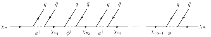
Figure 1: A decay chain in which an ensemble constituent $\chi_{n}$ experiences $S$ successive decays into increasingly lighter constituents. Each individual decay occurs through a three-body process of the form $\chi_{n_{k}}\rightarrow\bar{q}q\chi_{n_{k+1}}$ involving an off-shell $\phi^{\dagger}$ and resulting in the emission of two quarks (or parton-level “jets”). Each decay chain effectively terminates once a collider-stable constituent is reached.

Having parametrized the masses of our dark ensemble states $\chi_{n}$, we now turn to consider the manner in which these states interact with the particles of the visible-sector through a mediator. One possibility is that these interactions occur through an $s$-channel mediator $\phi$. Assuming that the SM fields $\psi$ which couple directly to $\phi$ are fermions, the interaction Lagrangian then takes the schematic form

$$\mathcal{L}_{\rm int}~{}=~{}\sum_{\psi}c_{\psi}\phi\bar{\psi}\psi+\sum_{m,n=0}^{N-1}c_{mn}\phi\bar{\chi}_{m}\chi_{n}~{},$$ (2)

where $c_{\psi}$ and $c_{mn}$ denote the couplings between the mediator and the fields of the visible and dark sectors, respectively. An alternative possibility is that these interactions take place via a $t$-channel mediator. The interaction Lagrangian in this case takes the schematic form

$$\mathcal{L}_{\rm int}~{}=~{}\sum_{\psi}\sum_{n=0}^{N-1}c_{\psi n}\phi^{\dagger}\bar{\chi}_{n}\psi+{\rm h.c.}$$ (3)

While both possibilities allow our dark-sector constituents $\chi_{n}$ to be produced at colliders — and also potentially allow these states to decay, with the simultaneous emission of visible-sector states OffDiagDM1 ; OffDiagDM2 — the mediator $\phi$ in the $t$-channel case can carry SM charges. If these include color charge, mediator particles can be copiously pair-produced on shell at hadron colliders, and decay cascades precipitated by the subsequent decays of these mediators can therefore contribute significantly to the signal-event rate in the detection channels which are our main interest in this paper. The interaction in Eq. (3) is also comparatively minimal, with the production and decay processes occurring through a single common interaction.

We shall therefore focus on the case of a $t$-channel mediator $\phi$ in this paper. In particular, we shall assume that each of the $\chi_{n}$ couples to an additional heavy scalar mediator particle $\phi$ of mass $m_{\phi}$ which transforms as a fundamental triplet under the $SU(3)_{c}$ gauge group of the SM and has hypercharge $Y_{\phi}=-2/3$. We shall then take the coupling between $\phi$ and each of the $\chi_{n}$ to be given by the interaction Lagrangian

$$\mathcal{L}_{\mathrm{int}}~{}=~{}\sum_{q}\sum_{n=0}^{N-1}\big{[}c_{nq}\phi^{\dagger}\bar{\chi}_{n}P_{R}q+\mathrm{h.c.}\big{]}~{},$$ (4)

where $q\in\{u,c,t\}$ denotes an up-type SM quark, where $P_{R}=\frac{1}{2}(1+\gamma^{5})$ is the usual right-handed projection operator, and where $c_{nq}$ is a dimensionless coupling constant which in principle depends both on the identity of the ensemble constituent and on the flavor of the quark. For concreteness, we shall assume that the $c_{nq}$ scale according to the power-law relation

$$c_{nq}~{}=~{}c_{0q}\left(\frac{m_{n}}{m_{0}}\right)^{\gamma}~{},$$ (5)

where the masses $m_{n}$ are given in Eq. (1), where $c_{0q}>0$ is an overall normalization for the couplings, and where $\gamma$ is a scaling exponent.

Generally speaking, the interaction Lagrangian in Eq. (4) can give rise to flavor-changing neutral currents (FCNCs), which are stringently constrained by data. However, such constraints can easily be satisfied. These issues will be discussed in greater detail in Sect. VII.

The interaction Lagrangian in Eq. (4) simultaneously describes two critical features of our model. First, we see that our mediator field generically allows the heavier ensemble constituents to decay to successively lighter constituents, thereby forming a decay chain. Indeed, according to our interaction Lagrangian, each step of the decay chain proceeds through an effective three-body decay process of the form $\chi_{k}\rightarrow q\overline{q}^{\prime}\chi_{\ell}$ involving an off-shell mediator $\phi$ particle, where $m_{\ell}<m_{k}$. Such a decay chain is illustrated in Fig. 1, with each step of the decay resulting in two parton-level jets. Indeed, such a decay chain effectively terminates only when a collider-stable constituent is reached. If the parameters which govern our model are such that each ensemble constituent $\chi_{k}$ decays primarily to those daughters $\chi_{\ell}$ whose masses $m_{\ell}$ are only slightly less than $m_{k}$, relatively long decay chains involving multiple successive such decays can develop before a collider-stable constituent is reached, especially if the first constituent $\chi_{n}$ that is produced is relatively massive. In such cases, relatively large numbers of parton-level “jets” — i.e., quarks or gluons — can be emitted.

We see, then, that any $\chi_{n}$ that is produced — unless it happens to be collider-stable — will generate a subsequent decay chain. The only remaining issue therefore concerns the manner in which such $\chi_{n}$ particles might be produced at a hadron collider such as the LHC.  However, the relevant production processes are also described by our interaction Lagrangian in Eq. (4) in conjunction with our assumption that $\phi$ is an $SU(3)_{c}$ color triplet. Indeed, given this interaction Lagrangian, there are a number of distinct possibilities for how the production of the $\chi_{n}$ might take place:

• The $\chi_{n}$ may be produced directly via the process $pp\rightarrow\chi_{m}\bar{\chi}_{n}$ at leading order. The Feynman diagram for this process is shown in Fig. 4.

• The $\chi_{n}$ may be produced via the process $pp\rightarrow\phi\chi_{m}$, followed by a decay of the form $\phi\rightarrow q\bar{\chi}_{n}$. In such cases, one constituent $\chi_{n}$ particle is produced directly while the other results from a subsequent $\phi$ decay. Two representative Feynman diagrams for such processes are shown in Fig. 4.

• Finally, because the $\phi$ particles are $SU(3)_{c}$ triplets, the $\chi_{n}$ may also be produced via the process $pp\rightarrow\phi^{\dagger}\phi$ followed by decays of the form $\phi\rightarrow q\bar{\chi}_{n}$ and $\phi^{\dagger}\rightarrow\chi_{m}\bar{q}$. In such cases, both $\chi_{m}$ and $\bar{\chi}_{n}$ are produced via the decays of $\phi$ particles. A representative Feynman diagram for such a process is shown in Fig. 4.

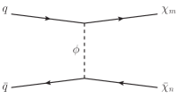
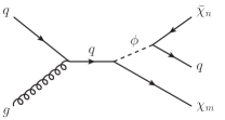
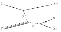
Figure 2: Feynman diagram for the process in which $\chi_{m}$ and $\overline{\chi}_{n}$ are produced directly via the process $pp\rightarrow\chi_{m}\bar{\chi}_{n}$.

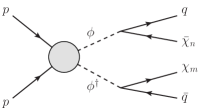
Figure 3: Representative Feynman diagrams for collider processes in which the initial production process $pp\rightarrow\phi\chi_{m}$ is followed by a decay of the form $\phi\rightarrow q\bar{\chi}_{n}$.

Figure 4: Representative Feynman diagram for collider processes in which $pp\rightarrow\phi^{\dagger}\phi$ production is followed by decays of the form $\phi\rightarrow q\bar{\chi}_{n}$ and $\phi^{\dagger}\rightarrow\chi_{m}\bar{q}$.

These different production processes have very different phenomenologies. For example, since the amplitude for each contributing diagram in Fig. 4 is proportional to the product $c_{m}c_{n}$, the cross-section — and therefore the event rate — for the overall process is proportional to $c_{0}^{4}$. By contrast, the event rates for the overall processes in Fig. 4 are proportional to $c_{0}^{2}$ when $\phi$ is on shell, since the factor $c_{n}$ from the decay vertex affects the decay width of $\phi$ but not the cross-section for $pp\rightarrow\phi\chi_{m}$. Finally, the event rate for the process shown in Fig. 4 is essentially independent of $c_{0}$, as $\phi$ is an $SU(3)$ color triplet and can therefore be pair-produced through diagrams involving strong-interaction vertices alone.

Another distinction between these processes is the manner in which their overall cross-sections scale with the number of kinematically accessible components $\chi_{n}$ within the ensemble. For example, the event rate for the process shown in Fig. 4 is essentially set by the cross-section for the initial process $pp\to\phi^{\dagger}\phi$ and is thus largely insensitive to the multiplicity of states within the ensemble. By contrast, processes such as those shown in Figs. 4 and 4 scale with the multiplicity of the $\chi_{n}$ states that are kinematically accessible, as the contributions from the production of each separate constituent $\chi_{n}$ must be added together. For large ensembles, this can lead to a significant enhancement of the total cross-sections for such processes.

All of these processes are capable of giving rise to large numbers of parton-level jets, particularly if the $\chi_{n}$ that are produced give rise to long subsequent decay chains. Additional parton-level jets may also be produced as initial-state radiation or radiated off any internal lines associated with strongly-interacting particles. However, these different processes differ in the minimum numbers of parton-level jets which may be produced. For example, the direct-production process in Fig. 4 can in principle be entirely jet-free as long as only collider-stable ensemble constituents are produced. Likewise, the processes in Fig. 4 must give rise to at least one jet, and indeed processes of this form involving an on-shell $\phi$ particle often turn out to provide the dominant contribution to the $pp\rightarrow\chi_{m}\bar{\chi}_{n}+j$ monojet production rate at the LHC within our model. By contrast, the process in Fig. 4 must give rise to at least two jets.

In order to streamline the analysis of our model, we shall make two further assumptions in what follows. First, we shall assume that the $\chi_{n}$ couple only to the up quark, taking $c_{0q}=0$ for $q=\{c,t\}$. Thus only the $c_{nu}$ coefficients are non-zero, and we shall henceforth adopt the shorthand notation $c_{n}\equiv c_{nu}$ for all $n$. Alternative coupling structures shall be discussed in Sect. VII. Second, we shall assume that $N$, the total number of constituents in our ensemble, is not only finite but also chosen so as to maximize the size of the ensemble while nevertheless ensuring that all of the ensemble constituents $\{\chi_{0},\chi_{1},...,\chi_{N-1}\}$ are kinematically accessible via the decays of $\phi$. In other words, we shall take $N$ to be the largest integer such that

$$N~{}\leq~{}1+\left(\frac{m_{\phi}-m_{0}-m_{q}}{\Delta m}\right)^{1/\delta}~{},$$ (6)

where $m_{q}$ is the mass of the final-state (up) quark. While this last assumption is not required for the self-consistency of our model, we shall see that it simplifies the resulting analysis and leads to an interesting phenomenology.

With these simplifications, our framework is characterized by six free parameters: $\{m_{0},\Delta m,\delta,m_{\phi},c_{0},\gamma\}$. These six parameters determine the masses of the ensemble constituents $\chi_{n}$, the probabilities for producing these different ensemble constituents from the decays of $\phi$, and the branching fractions that govern the possible subsequent decays of these constituents. Indeed, depending on the values of these parameters, many intricate patterns of potential decay chains are possible which collectively contribute to jet production. For example, in some regions of parameter space, the lifetimes of the heavier ensemble states are shorter than those of the lighter states, while in other regions the opposite is true. Of course, the lightest state receives no contribution to its width from the interaction Lagrangian in Eq. (4) and is therefore either absolutely stable or else decays only as a result of additional, highly suppressed interactions on a timescale that far exceeds collider timescales. Likewise, in some regions of parameter space, each $\chi_{n}$ preferentially decays to daughters $\chi_{\ell}$ for which $m_{\ell}\ll m_{n}$, while in other regions the preferred daughters $\chi_{\ell}$ are only slightly lighter than $\chi_{n}$. Finally, in some regions of parameter space, the contributions to jet production coming from the processes illustrated within Figs. 4 and 4 might dominate, while in other regions of parameter space the contributions from the process illustrated within Fig. 4 might dominate. Thus, even though our framework is governed by only the single interaction in Eq. (4), this framework is extremely rich and many different resulting phenomenologies are possible.

In our analysis of this framework, we shall be interested primarily in those regions of parameter space which potentially give rise to extended jet cascades at colliders such as the LHC.  We shall therefore be interested in those regions of parameter space that give rise to a relatively large number of kinematically accessible ensemble constituents $\chi_{n}$ which decay promptly on collider timescales and for which the corresponding decays occur along decay chains involving a relatively large number of steps. Beyond this, however, we will not make any further assumptions concerning the values of these parameters. Of course, within our parameter-space regions of interest, there may exist subregions in which some of the other constituents will have very long lifetimes — lifetimes which potentially exceed the age of the universe. In such cases, these long-lived constituents might serve as potential dark-matter candidates of the sort intrinsic to the Dynamical Dark Matter framework DDM1 ; DDM2 , with the decay cascades arising from the decays of the shorter-lived ensemble constituents potentially serving as a signature of this framework. Since our focus in this paper is on the collider phenomenology of the mediator-induced decay chains that arise in this model, we make no additional assumption as to whether the $\chi_{n}$ collectively contribute a non-negligible fraction of the overall present-day dark-matter abundance. However, we comment on the possibility that the $\chi_{n}$ might contribute significantly to this abundance in Sect. VII.

III Decay-Chain Phenomenology and the Generation of Extended Jet Cascades

We shall now demonstrate that the model presented in Sect. II is capable of giving rise to extended jet cascades at the LHC.  In this section our analysis shall be purely at the parton level, while in Sect. IV we shall pass to the detector level.

In principle, mediator-induced decay cascades can arise from any of the processes illustrated in Figs. 4–4. Of course, our eventual goal in this paper is not merely to demonstrate that cascades of this sort with large jet multiplicities are possible, but that they might emerge while simultaneously satisfying existing LHC monojet and multi-jet constraints. For this, of course, the contributions from all of the processes discussed in Sect. II will ultimately matter. This will be discussed in Sect. VI.

We shall begin by outlining the kinematics and combinatorics of the mediator-induced decay chains precipitated by the production processes illustrated in Figs. 4–4. We shall then discuss how the emergence of extended decay chains yielding large numbers of jets depends on the parameters which characterize our model, and identify a region of parameter space within which such extended decay chains emerge naturally while satisfying certain internal self-consistency constraints.

III.1 The structure of the decay chain: Kinematics and combinatorics

Each of the processes illustrated in Figs. 4–4 eventually results in decay chains of the sort illustrated in Fig. 1. In cases such as that illustrated in Fig. 4, our ensemble constituents $\chi_{m}$ and $\overline{\chi}_{n}$ are produced directly. Each then becomes the heaviest component of a subsequent decay chain. By contrast, in cases such as that illustrated in Fig. 4, the particles that are produced directly are the mediator particles $\phi$ and $\phi^{\dagger}$. It is the subsequent decays of these mediators which then trigger the unfolding of our decay chains. Finally, cases such as those illustrated in Fig. 4 exhibit what may be considered a “mixture” between these two production mechanisms.

In this section, rather than analyze each process separately, we shall instead treat them together by focusing on the two primary classes of decays which establish and sustain their decay chains. These are

$$\phi^{\dagger}~{} \rightarrow ~{}\overline{q}\,\chi_{n}$$

$$\chi_{n}~{} \rightarrow ~{}\overline{q}^{\prime}q\,\chi_{\ell}~{}.$$ (7)

Note that although we have written these decay processes in generality, we shall — as discussed in Sect. II — restrict our attention to the case in which all quarks participating in these processes are up-quarks (i.e., $q=q^{\prime}=u$) in what follows. For cases involving the initial production of a mediator $\phi$, the first process in Eq. (7) in some sense “initializes” the decay chain by producing the heaviest $\chi_{n}$ constituent within the chain. This initialization process simultaneously produces one jet. The second process then iteratively generates the subsequent decays — each producing two jets — which collectively give rise to the decay chain through which this heaviest constituent $\chi_{n}$ sequentially decays into lighter constituents. By contrast, for cases involving the direct production of an ensemble constituent $\chi_{n}$, only the second process in Eq. (7) is relevant for generating the subsequent decay chain.

Even with a fixed initial state, each of the decay processes in Eq. (7) can result in a variety of different daughter particles. Indeed, starting from a given mediator particle $\phi$, it is possible for any kinematically-allowed constituent $\chi_{n}$ to be produced via the first process, each with a different probability. Likewise, a given $\chi_{n}$ can generally decay into any lighter constituents via the second process, with each possible daughter state occurring with a different probability as well. The sequential repetitions of this latter process thus lead to a proliferation of independent decay chains, with each decay chain terminating only when the lightest ensemble constituent is ultimately reached. (For practical purposes we may also consider a given decay chain to have effectively terminated if the lifetimes for further decays exceed collider timescales.) Thus, combining these effects, we see that each of the processes sketched in Figs. 4–4 actually spawns a large set of many different possible decay chains, each with its own relative probability for occurring and each potentially producing a different number of jets.

It is not difficult to study these decay chains analytically. Within any particular region of the model parameter space, the first step is to calculate the partial widths $\Gamma_{\phi n}\equiv\Gamma(\phi^{\dagger}\rightarrow\bar{q}\chi_{n})$ and $\Gamma_{n\ell}\equiv\Gamma(\chi_{n}\rightarrow\bar{q}^{\prime}q\chi_{\ell})$ associated with the processes in Eq. (7). With $q=q^{\prime}=u$ and with the up-quark treated as having a negligible mass, we find that $\Gamma_{\phi n}$ for any $n\leq N-1$ is to a very good approximation given by

$$\Gamma_{\phi n}~{}=~{}\frac{c_{n}^{2}}{16\pi}\frac{(m_{\phi}^{2}-m_{n}^{2})^{2}}{m_{\phi}^{3}}~{}.$$ (8)

Likewise, we find that $\Gamma_{n\ell}$ takes the form

$$\Gamma_{n\ell}~{} = ~{}\frac{3c_{n}^{2}c_{\ell}^{2}}{256\pi^{2}}\frac{m_{\phi}}{r_{\phi n}^{3}}\Bigg{[}f_{\phi n\ell}^{(1)}-f_{\phi n\ell}^{(2)}\ln(r_{n\ell})$$ (9)

$$~{}~{}+f_{\phi n\ell}^{(3)}\ln\left(\frac{1-r_{\phi n}^{2}}{1-r_{\phi n}^{2}r_{n\ell}^{2}}\right)\Bigg{]}~{},$$

where $r_{ij}\equiv m_{j}/m_{i}$, where $r_{\phi n}\equiv m_{n}/m_{\phi}$, and where

$$f_{\phi n\ell}^{(1)}~{} \equiv ~{}6r_{\phi n}^{2}(1-r_{n\ell}^{2})-5r_{\phi n}^{4}(1-r_{n\ell}^{4})$$

$$~{}+2r_{\phi n}^{6}r_{n\ell}^{2}(1-r_{n\ell}^{2})$$

$$f_{\phi n\ell}^{(2)}~{} \equiv ~{}4r_{\phi n}^{8}r_{n\ell}^{4}$$

$$f_{\phi n\ell}^{(3)}~{} \equiv ~{}6-8r_{\phi n}^{2}(1+r_{n\ell}^{2})-2r_{\phi n}^{8}r_{n\ell}^{4}$$

$$~{}+2r_{\phi n}^{4}(1+4r_{n\ell}^{2}+r_{n\ell}^{4})~{}.$$ (10)

Under the assumption that no additional interactions beyond those in Eq. (7) contribute non-negligibly to the total width of either $\phi$ or the $\chi_{n}$, the total decay width $\Gamma_{\phi}$ of $\phi$ is then simply

$$\Gamma_{\phi}~{}=~{}\sum_{n=0}^{N-1}\Gamma_{\phi n}~{},$$ (11)

with a corresponding $\phi$ lifetime $\tau_{\phi}\equiv 1/\Gamma_{\phi}$. Likewise, the total decay width $\Gamma_{n}$ for each ensemble constituent $\chi_{n}$ is simply

$$\Gamma_{n}~{}=~{}\sum_{\ell=0}^{n-1}\Gamma_{n\ell}~{},$$ (12)

with a corresponding constituent lifetime $\tau_{n}\equiv 1/\Gamma_{n}$. As discussed in Sect. II, the lightest ensemble constituent $\chi_{0}$ receives no contribution to its width from the interaction Lagrangian in Eq. (4) and is therefore assumed to be stable on collider timescales. Of course, the results in Eqs. (8) and (9) assume that the $\phi$ and $\chi_{n}$ particles have total decay widths which are relatively small compared with their masses. This is a self-consistency constraint which will ultimately be found to hold across our eventual parameter-space regions of interest.

While $\Gamma_{\phi}$ and $\Gamma_{n}$ determine the overall timescales for particle decays within our model, it is the branching fractions $\mathrm{BR}_{\phi n}\equiv\Gamma_{\phi n}/\Gamma_{\phi}$ and $\mathrm{BR}_{n\ell}\equiv\Gamma_{n\ell}/\Gamma_{n}$ which effectively determine the probabilities associated with the various possible decay chains that can arise. The behavior of these branching fractions is essentially determined by the interplay between two factors. The first of these factors is purely kinematic in origin and arises due to phase-space considerations which suppress the partial widths for decays involving heavier ensemble constituents in the final state. Thus, this factor always decreases as the index which labels this final-state ensemble constituent increases. The second factor arises as a result of the scaling of the individual coupling constants $c_{n}$ in Eq. (5) across the ensemble. Depending on the value of the scaling exponent $\gamma$, this factor may either increase or decrease with the final-state index.

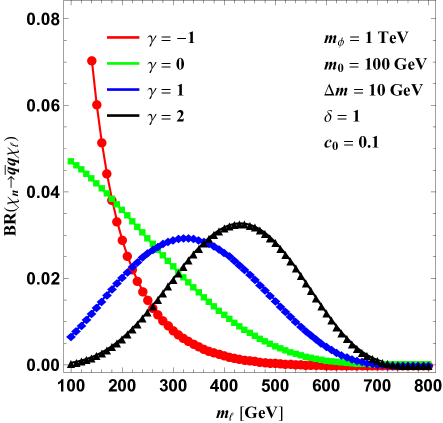
Figure 5: The branching fraction $\mathrm{BR}_{n\ell}$ for a decaying ensemble constituent $\chi_{n}$, plotted as a function of the daughter mass $m_{\ell}$ for different values of the scaling exponent $\gamma$. The results shown here correspond to the parameter values $n=70$, $m_{\phi}=1$ TeV, $m_{0}=100$ GeV, $\Delta m=10$ GeV, $\delta=1$, and $c_{0}=0.1$ — a choice of parameters for which the mass of the parent is $m_{n}=800$ GeV.  We see that when $\gamma$ is large (even if only moderately so), the couplings $c_{\ell}$ which increase with $\ell$ are able to partially overcome the increasingly severe phase-space suppressions that also arise for larger $\ell$, allowing the parent $\chi_{n}$ to decay preferentially to daughters $\chi_{\ell}$ with intermediate values of $\ell$. This phenomenon underpins the existence of decay chains with many intermediate steps, allowing such long decay chains to dominate amongst the set of all possible decay chains that emerge from a given parent $\chi_{\ell}$.

In the regime in which $\gamma\lesssim 0$, the mediator $\phi$ and all of the $\chi_{n}$ decay preferentially to $\chi_{\ell}$ with relatively small values of $\ell$. Thus, for these parameters, the corresponding decay chains typically involve only one or a few steps and do not give rise to large multiplicities of jets. By contrast, in the opposite regime in which $\gamma$ is positive and sufficiently large that the enhancement in $c_{\ell}^{2}$ with increasing $\ell$ overcomes the phase-space suppression, decays to $\chi_{\ell}$ with intermediate values of $\ell$ are preferred. Within this regime, long decay chains can develop and events involving large numbers of hadronic jets naturally arise.

In Fig. 5, we plot $\mathrm{BR}_{n\ell}$ as a function of the daughter-particle mass $m_{\ell}$ for several different choices of $\gamma$, holding $n$ fixed. For these plots we have chosen the illustrative values $m_{\phi}=1$ TeV, $m_{0}=100$ GeV, $\Delta m=10$ GeV, $\delta=1$, and $c_{0}=0.1$. We have also chosen $n=70$ for the parent, implying a parent mass $m_{n}=800$ GeV.  On the one hand, we observe from Fig. 5 that $\mathrm{BR}_{n\ell}$ indeed decreases monotonically with $\ell$ for negative $\gamma$ — and indeed even for $\gamma=0$ — as expected. On the other hand, we also observe that decays to final states with $\ell>0$ are strongly preferred even for $\gamma=1$. Thus, even a moderate positive value of $\gamma$ is sufficient to ensure that decay cascades with multiple steps will be commonplace. Indeed, the shapes of the curves in Fig. 5 do not depend sensitively on the chosen values of $\Delta m$ or $\delta$ as long as the number of constituents $\chi_{\ell}$ lighter than $\chi_{n}$ is sufficiently large. This is because for fixed $m_{\phi}$ and $m_{n}$, the branching fraction $\mathrm{BR}_{n\ell}$ can be viewed as a function of the single variable $r_{n\ell}$. Thus, while changing $\Delta m$ and $\delta$ changes the values of $r_{n\ell}$ at which this function is evaluated, it has no effect on form of the function itself.

Given our results for the relevant branching fractions, we now have the ingredients with which to calculate the probabilities associated with particular sequences of decays — i.e., particular decay chains — in our model. For simplicity, let us focus on the regime in which all $\chi_{n}$ with $n>0$ decay promptly within the detector. Under this assumption, each decay chain precipitated by the production of a given ensemble constituent effectively terminates only when $\chi_{0}$ (the lightest element within the ensemble) is produced. Within this regime, then, the probability $\mathcal{\hat{P}}(S)$ that such a decay chain will have precisely $S$ steps after the initial production of an ensemble constituent (i.e., the probability that our decay chain proceeds according to a schematic of the form $\chi_{n_{0}}\to\chi_{n_{1}}\to...\to\chi_{n_{S-1}}\to\chi_{0}$) is given by

$${\cal\hat{P}}(S)~{}=~{}\!\!\!\!\!\sum_{n_{0},n_{1},...,n_{S-1}=0}^{N-1}\!\!\!\!\!{\rm BR}_{n_{0}}^{\rm(prod)}{\rm BR}_{n_{0},n_{1}}\cdots{\rm BR}_{n_{S-1},0}~{}$$ (13)

for $0\leq S\leq N-1$, where we of course understand that ${\rm BR}_{ij}=0$ for all $j\geq i$ and where the initial factor ${\rm BR}_{n_{0}}^{\rm(prod)}$ is the relative probability that the specific ensemble constituent $\chi_{n_{0}}$ is originally produced. This last factor depends on the production process, with ${\rm BR}^{\rm(prod)}_{n_{0}}={\rm BR}_{\phi n_{0}}$ in the case of indirect production through the mediator $\phi$ and ${\rm BR}^{\rm(prod)}_{n_{0}}=1$ for direct $\chi_{n_{0}}$ production.

This result then allows us to calculate the probabilities $P(N_{\mathrm{jet}})$ that each of the processes in Figs. 4–4 yields precisely $N_{\mathrm{jet}}$ jets at the parton level. First, we observe that each of these processes directly or indirectly gives rise to two ensemble constituents $\chi_{n}$ and $\overline{\chi}_{m}$. While producing these ensemble constituents, each process also produces a certain number $\zeta$ of parton-level jets; indeed $\zeta=0,1,2$ for the processes sketched in Figs. 4, 4, and 4, respectively. Each of these two constituents then spawns a set of decay chains, with each step producing exactly two parton-level jets. Thus, for each process in Figs. 4–4, the corresponding probability $P(N_{\mathrm{jet}})$ that a single event will yield a specified total number $N_{\mathrm{jet}}$ of parton-level jets (from either quarks or anti-quarks) is therefore given by

$$P(N_{\mathrm{jet}})~{}=~{}\sum_{S_{1}=0}^{(N_{\mathrm{jet}}-\zeta)/2}\mathcal{\hat{P}}(S_{1})\,\mathcal{\hat{P}}(N_{\mathrm{jet}}/2-\zeta/2-S_{1})~{}.$$ (14)

Of course, for each process $N_{\mathrm{jet}}$ is restricted to the values $\zeta+n$ where $0\leq n\leq 4N-4$, $n\in 2\mathchoice{\hbox{\cmss Z\kern-3.99994ptZ}}{\hbox{\cmss Z\kern-3.99994ptZ}}{\lower 0.9pt\hbox{\cmsss Z\kern-2.79996ptZ}}{\lower 1.2pt\hbox{\cmsss Z\kern-2.79996ptZ}}$.

In Fig. 6, we plot $P(N_{\mathrm{jet}})$ as a function of $N_{\mathrm{jet}}$ for several different choices of the scaling exponent $\gamma$. For this figure we have again taken the illustrative values $m_{\phi}=1$ TeV, $m_{0}=100$ GeV, $\Delta m=10$ GeV, $\delta=1$, and $c_{0}=0.1$, which together imply $N=90$. For concreteness we have also chosen $\zeta=2$, corresponding to the process sketched in Fig. 4 for which ${\rm BR}^{\rm(prod)}_{n_{0}}={\rm Br}_{\phi,n_{0}}$. For this choice of parameters, we see that the decay cascades initiated by parent-particle decays can indeed give rise to significant numbers of jets at the parton level. Indeed, we observe from this figure that for $\gamma\gtrsim 1$, the majority of events in which a pair of mediator particles is produced have $N_{\mathrm{jet}}\gtrsim 10$. Similar results also emerge for the processes in Figs. 4 and 4.

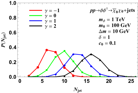
Figure 6: The probability $P(N_{\mathrm{jet}})$ for obtaining a total number $N_{\mathrm{jet}}$ of jets (i.e., quarks or anti-quarks) at the parton level from the decay of a pair of mediator particles $\phi$ and $\phi^{\dagger}$ as in Fig. 4, plotted as a function of $N_{\mathrm{jet}}$ for several different values of the scaling exponent $\gamma$. The red, green, blue, and black curves correspond to the choices $\gamma=\{-1,0,1,2\}$ for this parameter, respectively. The remaining model parameters have been assigned the benchmark values $m_{\phi}=1$ TeV, $m_{0}=100$ GeV, $\Delta m=10$ GeV, $\delta=1$, and $c_{0}=0.1$. The results shown in the figure indicate that large jet multiplicities can indeed arise within our framework — especially for large values of $\gamma$.

We conclude, then, that the example model described in Sect. II is capable of giving rise to extended jet cascades at the parton level. Indeed, the existence of this signature does not require any fine-tuning, and emerges as an intrinsic part of the phenomenology of the model.

III.2 Constraining the model parameter space

Our analysis in Sect. III.1 focused on the general kinematic and combinatoric structure of the decay chains that give rise to extended jet cascades in our model. However, there are a number of additional constraints which must also be addressed before we can claim that our model is actually capable of giving rise to signatures involving large jet multiplicities at a collider such as the LHC.  Some of these additional constraints are fairly generic, and can be discussed even at the parton level. Indeed, as we shall now demonstrate, satisfactorily addressing these concerns will enable us to place several important additional constraints on the parameter space of our model. However, other constraints are more phenomenological and process-specific, having to do with existing LHC bounds on monojet and multi-jet signatures. Discussion of these latter constraints will therefore be deferred to Sect. V.

As discussed in Sect. II, our model is described by six parameters: $\{m_{0},\Delta m,\delta,m_{\phi},c_{0},\gamma\}$. The first three of these parameters together describe the entire mass spectrum $m_{n}$ of the ensemble constituents, and the fourth is nothing but the mass $m_{\phi}$ of the mediator $\phi$. As we have seen, however, the all-important branching fractions ${\rm BR}_{\phi n}$ and ${\rm BR}_{n\ell}$ depend on only the ratios of these masses. Likewise, the quantity $N$ which sets an upper limit on the number of possible jets that can be produced (and which was defined in Sect. II as the number of ensemble constituents which are kinematically accessible via the decays of $\phi$) also implicitly depends on these ratios. Together, these considerations then govern the choices of mass ratios in our system.

However, this still leaves an overall mass scale which we may take to be $m_{\phi}$ itself. Likewise, we have not yet constrained the two parameters $c_{0}$ and $\gamma$ which together describe the spectrum of couplings in our model through Eq. (5). Of course, we have already seen in Figs. 5 and 6 that only when $\gamma$ is sufficiently positive and large do our decays preferentially proceed through sufficiently small steps that allow decay chains with sufficiently large numbers of steps to develop. However, this still leaves $m_{\phi}$ and $c_{0}$ unconstrained. Fortunately, there exist additional phenomenological constraints which will enable us to determine suitable ranges for these two remaining parameters as well.

First, although we have demonstrated how extended mediator-induced decay cascades might potentially emerge from our model, we must also ensure that the overall cross-sections for producing these cascades are sufficiently large that the resulting multi-jet signal could actually be detected over background. While these cross-sections are certainly affected by the cascade probabilities discussed above, their overall magnitudes are set by the simpler cross-sections associated with the sub-processes for the production of the initial states that trigger these cascades. For the diagrams sketched in Figs. 4–4, these production cross-sections are respectively given by

$$\sigma_{\chi\chi}~{} \equiv ~{}\sum_{m,n=0}^{N-1}\sigma(pp\to\chi_{m}\overline{\chi}_{n})~{}$$

$$\sigma_{\phi\chi}~{} \equiv ~{}\sum_{m=0}^{N-1}\sigma(pp\to\phi\chi_{m})~{}$$

$$\sigma_{\phi\phi}~{} \equiv ~{}\sigma(pp\to\phi^{\dagger}\phi)~{}.$$ (15)

Calculating these cross-sections is relatively straightforward, and in Fig. 7 we display our results as functions of $m_{\phi}$ for a center-of-mass (CM) energy of $\sqrt{s}=13$ TeV.  In particular, the solid curves correspond to the parameter choices $m_{0}=500$ GeV, $\Delta m=50$ GeV, $c_{0}=0.1$, and $\delta=1$ with $\gamma=1$, while the dashed curves correspond to the same values of $m_{0}$, $\Delta m$, $c_{0}$, and $\delta$, but with $\gamma=3$. We note that since $\sigma_{\phi\phi}$ has no dependence at leading order on the mass spectrum of the ensemble constituents (and therefore on the values of the parameters $m_{0}$, $\Delta m$, and $\gamma$), the corresponding curves for both of these parameter choices are identical. We also note that the wiggles which appear in the curves for $\sigma_{\chi\chi}$ and $\sigma_{\chi\phi}$, especially at small $m_{\phi}$, are the consequence of threshold effects which arise due to the discrete changes in $N$ that occur as $m_{\phi}$ changes, in accordance with Eq. (6).

We observe from Fig. 7 that the cross-section for $\phi\phi$ pair-production dominates for small $m_{\phi}$, but falls rapidly from $\sigma_{\phi\phi}\sim 500$ fb to $\sigma_{\phi\phi}\sim 10^{-3}$ fb as the mass of the mediator increases from $m_{\phi}=500$ GeV to $m_{\phi}=2500$ GeV.  By contrast, the cross-sections for the other two production processes either grow with $m_{\phi}$ or fall less sharply over the range of $m_{\phi}$ shown. This is primarily a consequence of the corresponding increase in $N$, which in turn results in more individual production processes involving different $\chi_{n}$. Since increasing $\gamma$ in turn increases the individual production cross-sections for the heavier $\chi_{n}$, both $\sigma_{\chi\chi}$ and $\sigma_{\phi\chi}$ are noticeably larger for $\gamma=3$ than for $\gamma=1$. We also note that across the entire range of $m_{\phi}$ shown, $\sigma_{\chi\chi}$ and $\sigma_{\phi\chi}$ are both larger than $0.01$ fb, indicating that these processes could potentially lead to observable signals at the LHC.

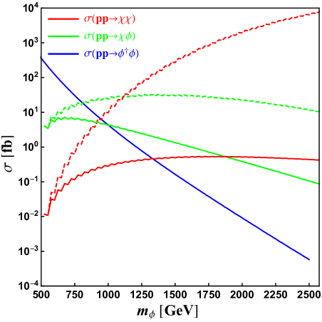
Figure 7: The three production cross-sections $\sigma_{\chi\chi}$, $\sigma_{\phi\chi}$, and $\sigma_{\phi\phi}$ in Eq. (15), plotted as functions of $m_{\phi}$ for $\sqrt{s}=13$ TeV.  The solid curves correspond to the parameter choices $m_{0}=500$ GeV, $\Delta m=50$ GeV, $c_{0}=0.1$, and $\delta=\gamma=1$, while the dashed curves correspond to the same parameter choices but with $\gamma=3$. We see that $\sigma_{\chi\chi}$ tends to dominate for large $m_{\phi}$, while $\sigma_{\phi\phi}$ tends to dominate for small $m_{\phi}$.

We now turn to examine how general considerations involving the coupling structure of our model serve to constrain the coupling parameter $c_{0}$. Since all of the couplings $c_{n}$ in our model are proportional to $c_{0}$, we see that $c_{0}$ serves as an overall proportionality factor for both $\Gamma_{\phi}$ and $\Gamma_{n}$. In particular, our results in Eqs. (8) and (9) imply that $\Gamma_{\phi}\propto c_{0}^{2}$ and $\Gamma_{n}\propto c_{0}^{4}$. Fortunately, the value of $c_{0}$ is constrained by a number of theoretical consistency conditions and phenomenological constraints. For example, given the perturbative treatment leading to the results in Eqs. (8) and (9), self-consistency requires that we must impose the perturbativity requirement that $c_{n}\lesssim 4\pi$ for all $0\leq n\leq N-1$. Given the general expression in Eq. (5), we see that the value of $c_{n}$ generally increases as a function of $n$ for $\gamma>0$ and decreases for $\gamma<0$. For any combination of model parameters we must therefore demand that

$$c_{0}~{}\lesssim~{}\begin{cases}4\pi\left[1+\frac{\Delta m}{m_{0}}(N-1)^{\delta}\right]^{-\gamma}&{\rm for}~{}~{}\gamma\geq 0\cr 4\pi&{\rm for}~{}~{}\gamma\leq 0~{}.\end{cases}$$ (16)

In addition, for cases in which the decay chains are initiated through the direct production of the mediator $\phi$, we are assuming that $\phi$ behaves like a physical particle rather than a broad resonance. We must therefore also demand that $c_{0}$ be sufficiently small that $\Gamma_{\phi}\ll m_{\phi}$, which in turn requires

$$c_{0}~{}\ll~{}4\sqrt{\pi}\left[\sum_{n=0}^{N-1}\left(\frac{m_{n}}{m_{0}}\right)^{\gamma}\left(1-\frac{m_{n}^{2}}{m_{\phi}^{2}}\right)^{2}\right]^{-1/2}$$ (17)

This latter constraint can occasionally surpass the one in Eq. (16). For example, for $\gamma=0$ we learn from Eq. (16) that $c_{0}\lower 3.01385pt\hbox{$\;\stackrel{{\scriptstyle\textstyle<}}{{\sim}}\;$}4\pi$, yet even in such cases $\Gamma_{\phi}$ can occasionally exceed $m_{\phi}$, even with only a few ensemble constituents.

In addition to these criteria for theoretical consistency, there are also a number of further constraints which we shall take into account in defining our region of interest within the full parameter space of our model. We emphasize that these are not necessarily inviolable constraints on the model, but rather conditions which we shall impose either for sake of clarity in simplifying our analysis or in order to restrict our focus within the model parameter space to regions in which long decay chains arise.

For example, in order for a decaying particle ensemble to give rise to observable signatures of mediator-induced decay cascades at the LHC, many of the $\chi_{n}$ constituents must of course decay promptly within the detector. In general, the decay length $L_{n}$ of $\chi_{n}$ in the detector frame is given by $L_{n}\equiv\beta\gamma c\tau_{n}$, where $\tau_{n}=\Gamma_{n}^{-1}$ is the proper lifetime of $\chi_{n}$ and where $\beta=v/c$ and $\gamma=(1-\beta^{2})^{-1/2}$ are the usual relativistic factors. Since we shall generally be interested in decay chains with many steps — chains in which the dominant individual decays produce daughters that are not overwhelmingly lighter than their parents — none of the ensemble constituents will be excessively boosted upon production. We can therefore treat the relativistic factor $\beta\gamma$ as a mere ${\cal O}(1)$ numerical coefficient in order to obtain an order-of-magnitude estimate of the bound. This is particularly convenient since these factors generally depend on the detailed structure of the decay chain and therefore differ from one event to the next. We will therefore estimate the characteristic length scale at which a given ensemble constituent decays as $c\tau_{n}$. Broadly speaking, if $c\tau_{n}\gg 1$ cm, a particle of species $\chi_{n}$ will typically appear as either a displaced vertex or as ${\hskip 2.56064pt/\hskip-6.544ptE_{T}}$ at the LHC.  By contrast, if $c\tau_{n}\lesssim\mathcal{O}(1\mathrm{~{}cm})$, such a particle will tend to decay promptly within the detector. It is these latter decays which are our focus.

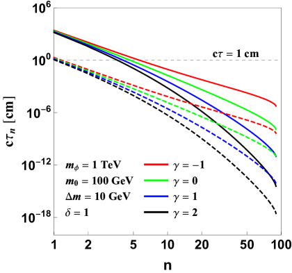
Figure 8: The decay lengths $c\tau_{n}$ of the ensemble constituents $\chi_{n}$, plotted as functions of $n$ for several different choices of model parameters. For all curves shown in this plot we have taken $m_{\phi}=1$ TeV, $m_{0}=100$ GeV, $\Delta m=10$ GeV, and $\delta=1$. The red, green, blue, and black curves correspond to the parameter choices $\gamma=\{-1,0,1,2\}$, respectively. Likewise, the solid curves correspond to the choice $c_{0}=0.02$, while the dashed curves correspond to the choice $c_{0}=0.1$. In general we see that increasing $c_{0}$ in this way has the effect of decreasing the decay lengths of our ensemble states and ultimately ensuring that all of the ensemble constituents decay within the detector.

In Fig. 8, we plot the length scales $c\tau_{n}$ as functions of $n$ for several different choices of model parameters. The red, green, blue, and black curves correspond to the parameter choices $\gamma=\{-1,0,1,2\}$, respectively. The solid curves correspond to the choice $c_{0}=0.02$, while the dashed curves correspond to the choice $c_{0}=0.1$. The values of the remaining model parameters are taken to be $m_{\phi}=1$ TeV, $m_{0}=100$ GeV, $\Delta m=10$ GeV, and $\delta=1$ for all curves shown. We emphasize that the perturbativity criterion in Eq. (16) is satisfied for all curves shown. Note that for the parameters shown, the decay lengths tend to decrease as functions of $n$. This remains true even if $\gamma=-1$, indicating that the total phase space available for the decays of $\chi_{n}$ increases with $n$ more rapidly than the associated couplings $c_{n}$ might decrease. For $c_{0}=0.02$, we see from Fig. 8 that a significant number of the ensemble constituents have $c\tau_{n}\gg{\cal O}(1~{}\mathrm{cm})$ and therefore do not decay promptly within the detector. Indeed, depending on the amount by which $c\tau_{n}$ exceeds ${\cal O}(1~{}{\rm cm})$, these $\chi_{n}$ would either decay a measurable distance away from the primary vertex (thereby giving rise to a displaced vertex), or else appear in the detector as ${\hskip 2.56064pt/\hskip-6.544ptE_{T}}$. By contrast, for $c_{0}=0.1$, we see that all $\chi_{n}$ with $n>0$ in the ensemble have $c\tau_{n}\lesssim\mathcal{O}(1~{}\mathrm{cm})$.

In general, long decay chains can certainly arise even in cases for which the lighter $\chi_{n}$ have values of $c\tau_{n}$ exceeding ${\cal O}(1~{}\mathrm{cm})$. In such cases the decays of relevance for our purposes would simply be the decays of the heavier constituents, with the decays of the lighter constituents subsequently occurring either with displaced vertices or completely outside the detector. Indeed, such situations could potentially give rise to many interesting signatures which will be discussed further in Sect. VIII.  However, for simplicity in what follows, we shall henceforth restrict our attention to the region of parameter space within which

$$c\tau_{n}~{}\lesssim~{}\mathcal{O}(1\mathrm{~{}cm})~{}~{}~{}{\rm for~{}all}~{}~{}n>0~{}.$$ (18)

In such cases, all possible decays of our ensemble constituents will occur within the detector, thereby allowing us to regard our decay chains as terminating only when the collider-stable ensemble “ground state” $\chi_{0}$ is reached.

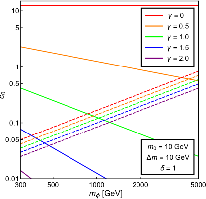
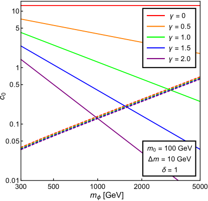
Figure 9: Allowed values of $c_{0}$ in our model, plotted as functions of $m_{\phi}$ for different values of $\gamma$. The results in both panels assume $\Delta m=10$ GeV and $\delta=1$, while $m_{0}=10$ GeV (top panel) or $m_{0}=100$ GeV (bottom panel). In each panel, the solid curves indicate the upper bounds on $c_{0}$ arising from the perturbativity constraint in Eq. (16), while the dashed curves indicate the lower bounds on $c_{0}$ arising from the prompt-decay constraint in Eq. (18). In general we see that there exists an ample allowed range for $c_{0}$ within which both constraints can be satisfied simultaneously, but this range becomes increasingly narrow as $m_{\phi}$ or $\gamma$ becomes large or as $m_{0}$ becomes small.

Since $\tau_{n}\propto c_{0}^{-4}$, requiring that our ensemble constituents satisfy the criterion in Eq. (18) is tantamount to imposing a lower bound on $c_{0}$ for any particular assignment of the remaining parameters which characterize our example model. Indeed, as illustrated in Fig 8, reducing $c_{0}$ below this bound only inhibits the decay rates of our ensemble constituents to a point beyond which some of the lighter ensemble constituents will begin to exhibit displaced vertices or decay outside the detector. However, since $c_{0}$ is also bounded from above by the perturbativity constraint in Eq. (16) and/or by our requirement that $\Gamma_{\phi}\ll m_{\phi}$, we see that there is a tension between these two groups of constraints.

In Fig. 9, we illustrate how the competition between the perturbativity constraint and the prompt-decay constraint play out within the parameter space of our model. The solid curves appearing within each panel of this figure represent the upper bounds on $c_{0}$ arising from the constraint in Eqs. (16) and (17), plotted as functions of $m_{\phi}$ for a variety of different values of $\gamma$. By contrast, the dashed lines represent the lower bounds on $c_{0}$ arising from our prompt-decay criterion in Eq. (18). While the contours in both panels in Fig. 9 correspond to $\Delta m=10$ GeV and $\delta=1$, those in the top panel correspond to the choice $m_{0}=10$ GeV while those in the bottom panel correspond to the choice $m_{0}=100$ GeV.

As is evident from Fig. 9, there are indeed regions of parameter space within which both the perturbativity constraint and the prompt-decay condition can be simultaneously satisfied. Nevertheless, it is also evident from this figure that as $\gamma$ increases, a significant tension rapidly develops between these two bounds. As we have already seen, the regions of parameter space within which $\gamma\gtrsim 1$ turn out to be the regions in which extended mediator-induced decay cascades develop. As a result, this tension will ultimately have important consequences for our model.

It is also relatively straightforward to understand the differences between the top and bottom panels of Fig. 9. In general, for $\gamma\geq 0$ the perturbativity constraint in Eq. (16) depends on the properties of $\chi_{N-1}$. By contrast, the prompt-decay condition in Eq. (18) depends on the properties of $\chi_{1}$. Given the functional form for $c_{n}$ in Eq. (5), we see that $c_{1}$ is essentially insensitive to $\gamma$ in the $\Delta m\ll m_{0}$ regime, as indicated in the bottom panel of Fig. 9. Likewise, the perturbativity bound becomes increasingly sensitive to $\gamma$ as the ratio $m_{N-1}/m_{0}$ increases.

For all of these reasons, we shall limit our attention in this paper to regions of parameter space in which $\gamma\lower 3.01385pt\hbox{$\;\stackrel{{\scriptstyle\textstyle>}}{{\sim}}\;$}1$, $c_{0}=0.1$. Indeed, as we have seen, these are the regions in which the processes illustrated in Figs. 4–4 can give rise to observable signatures involving relatively large numbers of jets at the parton level.

IV From Parton Level to Detector Level:  When You’re a Jet, Are You a Jet All the Way?

While it is certainly instructive to examine the collider phenomenology of our model at the parton level, what ultimately matters, of course, are the signatures that can actually be observed at the detector level. Indeed, not all of the parton-level “jets” produced from mediator-induced decay cascades at the parton level ultimately translate to individual reconstructed jets at the detector level. Moreover effects associated with initial-state radiation (ISR), final-state radiation (FSR), and parton-showering can give rise to additional jets at the detector level. Thus, it is critical that we investigate how the parton-level results we have derived in Sect. III are modified by these considerations at the detector level.

Toward this end, our analysis shall proceed as follows. For any given choice of model parameters, we generate signal events for the initial pair-production processes $pp\rightarrow\phi\chi_{m}$, $pp\rightarrow\chi_{m}\bar{\chi}_{n}$, and $pp\rightarrow\phi^{\dagger}\phi$ at the $\sqrt{s}=13$ TeV LHC using the MG5_aMC@NLO Alwall:2014hca code package. We then evaluate the cross-sections for these processes using this same code package. Due to the complexity of the decay chains which arise in our model, we treat the final-state particles produced during each step of the chain as being strictly on shell and simulate the decay kinematics using our own Monte-Carlo code. We have confirmed that the kinematic distributions obtained using our decay code agree well with those obtained from a full implementation of our model in MG5_aMC@NLO in cases in which the decay chains are short and such a comparison is feasible. The resulting set of three-momenta for the final-state particles in each event was then passed to Pythia 8 Sjostrand:2007gs for parton-showering and hadronization. Detector effects were simulated using Delphes 3 deFavereau:2013fsa . Jets were reconstructed in FastJet Cacciari:2011ma using the anti-$k_{T}$ clustering algorithm Cacciari:2008gp with a jet-radius parameter $R=0.4$.

This procedure has the practical benefit of allowing us to examine the kinematics of long decay chains. However, it is important to note that this procedure neglects certain considerations which can slightly modify the kinematics of the decay cascades and have $\mathcal{O}(1)$ effects on the cross-sections for the relevant final states. First, our procedure neglects the interference between two distinct contributions to the overall amplitude for the process $pp\rightarrow\chi_{m}\bar{\chi}_{n}+j$, the first coming from $pp\rightarrow\phi\chi_{m}$ production followed by the decay $\phi\rightarrow\bar{\chi}_{n}j$ of the on-shell $\phi$ particle, and the second coming from processes similar to $pp\rightarrow\chi_{m}\bar{\chi}_{n}$, but in which an additional quark or gluon is produced as initial-state radiation or radiated off the internal $\phi$ line. However, since we find that the former contribution vastly dominates the latter, the effect of neglecting these interference effects is not expected to be significant. Second, our procedure does not employ any jet-matching scheme in order to correct for double-counting in regions of phase space populated both by matrix-element-generation and parton-showering algorithms. Since the event-selection criteria we impose in our detector-level analysis involve significant threshold cuts on the $p_{T}$ values of the relevant jets, this effect is not expected to have a significant impact on our results. Third, our procedure also ignores the possibility that any $\chi_{n}$ which appear in decay chains or any of the mediators produced by the processes $pp\rightarrow\phi\chi_{m}$ or $pp\rightarrow\phi^{\dagger}\phi$ could be off shell. Once again, the impact on our results is not expected to be significant.

We begin by examining several experimental observables which are potentially useful for discriminating between signal and SM backgrounds. Clearly, the most distinctive feature of these extended mediator-induced decay cascades is the sheer multiplicity of “jets” at the parton level. Thus, given limited statistics, observables which characterize the overall properties of the event as a whole are likely to provide more distinguishing power than the observables which involve particular combinations of the momenta of individual jets in the event, due to the combinatorial issues associated with the latter. We therefore focus primarily on the former class of observables in what follows. These observables include $N_{\mathrm{jet}}$ and ${\hskip 2.56064pt/\hskip-6.544ptE_{T}}$, the distributions of the magnitude $p_{T_{j}}$ of the transverse momentum of all jets in the event, and the scalar sum

$$H_{T}~{}=~{}\sum_{j=1}^{N_{\mathrm{jet}}}p_{T_{j}}~{}.$$ (19)

In order to assess the extent to which showering, hadronization, and detector effects modify the distributions of $p_{T_{j}}$, $N_{\mathrm{jet}}$, ${\hskip 2.56064pt/\hskip-6.544ptE_{T}}$, and $H_{T}$, it is useful to compare the parton-level distributions of these observables to the corresponding detector-level distributions. In constructing the parton-level distributions of all of these collider observables, we consider each quark and anti-quark in the final state to be a “jet”, regardless of its proximity in $(\eta_{j},\phi_{j})$-space to any other such “jets” in the event, where $\eta_{j}$ and $\phi_{j}$ respectively denote the pseudorapidity and azimuthal angle of a given jet. Moreover, we impose no cuts on either $p_{T_{j}}$ or $\eta_{j}$. By contrast, in constructing the detector-level distribution of $p_{T_{j}}$, we require that every jet in a given event satisfy $p_{T_{j}}>20$ GeV and $|\eta_{j}|<5$. Furthermore, in order to be counted as a jet at the detector level, a would-be jet must be separated from every other, more energetic jet in the event by a distance $\Delta R_{jj}\equiv\sqrt{(\Delta\eta_{jj})^{2}+(\Delta\phi_{jj})^{2}}>0.4$ in $(\eta_{j},\phi_{j})$-space.

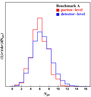
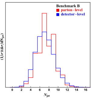
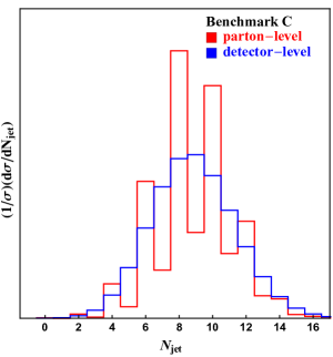
Figure 10: Normalized $N_{\mathrm{jet}}$ distributions for Benchmarks A (left panel), B (middle panel), and C (right panel). The red histogram in each panel shows the distribution obtained at the parton level (with quarks, anti-quarks, and gluons considered to be “jets”), while the blue histogram shows the corresponding distribution at the detector level.

For purposes of illustration, we identify three representative benchmark points within the parameter space of this model for which these criteria discussed in Sec. III.2 are satisfied, but for which different classes of production processes dominate the event rate in the multi-jet channel at large $N_{\mathrm{jet}}$. The parameter choices associated with these benchmarks are provided in Table 1.  Benchmark A is representative of the regime in which both $pp\rightarrow\phi^{\dagger}\phi$ and $pp\rightarrow\phi\chi_{m}$ provide significant contributions to the event rate in the multi-jet channel at large $N_{\mathrm{jet}}$, with these two processes contributing at roughly the same order. Benchmark B is representative of the regime in which $pp\rightarrow\phi\chi_{m}$ dominates the event rate, while Benchmark C is representative of the regime in which $pp\rightarrow\chi_{m}\bar{\chi}_{n}$ dominates.

In Fig. 10, we show the normalized distributions of $N_{\mathrm{jet}}$ obtained for Benchmarks A (left panel), B (middle panel), and C (right panel). The distributions shown include the individual contributions from $pp\rightarrow\phi\chi_{m}$, $pp\rightarrow\chi_{m}\bar{\chi}_{n}$, and $pp\rightarrow\phi^{\dagger}\phi$, each weighted by the cross-section for the corresponding process. The red histogram in each panel shows the distribution obtained at the parton level (with quarks, anti-quarks, and gluons considered to be “jets”), while the blue histogram shows the corresponding distribution at the detector level.

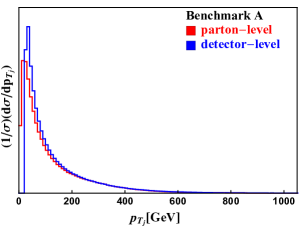
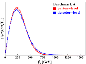
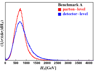
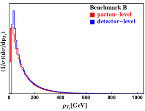
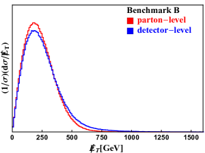
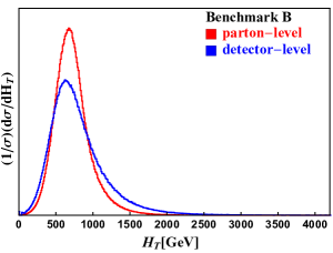
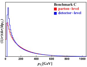
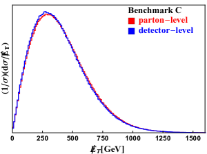
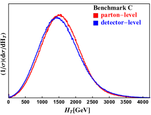
Figure 11: Normalized distributions of $p_{T_{j}}$ (left column), ${\hskip 2.56064pt/\hskip-6.544ptE_{T}}$ (middle column), and $H_{T}$ (right column) for the three parameter-space benchmarks defined in Table 1.  The distributions in the top, middle, and bottom rows of the figure correspond to Benchmarks A, B, and C, respectively. The red histogram in each panel shows the distribution obtained at the parton level (with quarks, anti-quarks, and gluons considered to be “jets”), while the blue histogram shows the corresponding distribution at the detector level.

For Benchmark A, we see from Fig. 10 that the parton-level and detector-level $N_{\mathrm{jet}}$ distributions look quite similar and that both of these distributions peak at around $N_{\mathrm{jet}}=6$. For Benchmark B, by contrast, the parton-level distribution exhibits local maxima at both $N_{\mathrm{jet}}=7$ and at $N_{\mathrm{jet}}=9$. This behavior follows from the fact that processes of the form $pp\rightarrow\phi\chi_{n}$, which yield an odd number of parton-level jets, dominate the production cross-section for this benchmark. Moreover, we observe that in going from the parton level to the detector level, the $N_{\mathrm{jet}}$ distribution shifts to slightly lower values. Several effects contribute to this reduction in $N_{\mathrm{jet}}$. First, jets associated with soft, isolated quarks or anti-quarks may fall below the $p_{T_{j}}>20$ GeV detector-level threshold for jet identification. Moreover, due to the large multiplicity of jets in these events, the hadrons associated with one or more of these jets frequently end up in such close proximity in $(\eta_{j},\phi_{j})$ space that they will be clustered together as a single jet at the detector level. For Benchmark C, the parton-level $N_{\mathrm{jet}}$ distribution peaks around $N_{\mathrm{jet}}=10$, with most of the final states containing even numbers of jets. The distribution is smoothed out at the detector level, but otherwise retains the same overall shape.

Benchmark	$m_{\phi}$	$m_{0}$	$\Delta m$	$\delta$	$\gamma$	$c_{0}$
A	1 TeV	500 GeV	50 GeV	1	1	0.1
B	1 TeV	500 GeV	50 GeV	1	3	0.1
C	2 TeV	500 GeV	50 GeV	1	1.5	0.1

Table 1: Parameter choices which define our three representative benchmark points. Benchmark A is representative of the regime in which $pp\rightarrow\phi^{\dagger}\phi$ and $pp\rightarrow\phi{\chi}_{m}$ both contribute significantly (and at roughly the same order) to the event rate. By contrast, Benchmark B is representative of the regime in which $pp\rightarrow\phi{\chi}_{m}$ dominates the event rate. Benchmark C is representative of the regime in which $pp\rightarrow\chi_{m}\bar{\chi}_{n}$ dominates.

One of the primary messages of Fig. 10 is that our benchmarks all give rise to a significant population of events with large jet multiplicities even at the detector level. Indeed, for Benchmarks A, B, and C, we find that the fraction of events for which $N_{\mathrm{jet}}\geq 9$ at the detector level is $16.3\%$, $24.3\%$, and $54.8\%$, respectively.

In Fig. 11, we show the normalized distributions for the other collider observables we consider in our analysis for our three parameter-space benchmarks. From left to right, the panels in each row of the figure correspond to the observables $p_{T_{j}}$, ${\hskip 2.56064pt/\hskip-6.544ptE_{T}}$, and $H_{T}$. The distributions in the top, middle, and bottom rows of the figure correspond to Benchmarks A, B, and C, respectively. The red histogram in each panel once again shows the distribution obtained at the parton level, while the blue histogram shows the corresponding distribution at the detector level.

In interpreting the results displayed in Fig. 11, we begin by noting that the parton-level $p_{T_{j}}$ distributions for all of our benchmarks are sharply peaked toward small values of $p_{T_{j}}$. In other words, as one might expect, given the length of the decay chains in these decay-cascade scenarios, a significant fraction of the quarks and anti-quarks produced in these decay chains tend to be extremely soft. However, we also note that the distributions for Benchmarks A and B are more sharply peaked than the distribution for Benchmark C.  This is ultimately a result of $m_{\phi}$ being larger for this latter benchmark than for the other two. A larger value of $m_{\phi}$ implies a larger value of $N$, and the fact that $\gamma>0$ for Benchmark C implies that production processes involving the heavier $\chi_{n}$ present in the ensemble will dominate. The average CM energy associated with any of the production processes in Figs. 4–4 is consequently larger for Benchmark C than it is for Benchmark A or B, which results in a higher average $p_{T_{j}}$. We also observe that since a $p_{T_{j}}>20$ GeV threshold is required for jet identification at the detector level, many of the soft “jets” present at the parton level for each of our benchmarks do not translate into jets at the detector level.

In comparison with the $p_{T_{j}}$ distributions shown in Fig. 11, the corresponding ${\hskip 2.56064pt/\hskip-6.544ptE_{T}}$ and $H_{T}$ distributions vary more dramatically from one benchmark to the next. Perhaps not unsurprisingly, the parton-level $H_{T}$ distribution for Benchmark C peaks at a higher value $H_{T}$ than do the distributions of this same variable for Benchmarks A and B, again owing to the fact that $m_{\phi}$ is larger for this benchmark. More interestingly, however, we also see that the parton-level and detector-level $H_{T}$ distributions for Benchmark C are almost identical, while the detector-level $H_{T}$ distributions for Benchmarks A and B differ drastically from the corresponding distributions at parton level. The discrepancy between the parton-level and detector-level $H_{T}$ distributions for these two benchmarks is ultimately a result of the $p_{T_{j}}>20$ GeV threshold for jet-identification at the detector level. As discussed above, the jets produced through mediator-induced decay cascades have a higher average $p_{T_{j}}$ for Benchmark C than they do for Benchmarks A or B, and consequently the $H_{T}$ distribution for this benchmark is affected less by the cuts. A similar effect, albeit less pronounced, is also observed in the ${\hskip 2.56064pt/\hskip-6.544ptE_{T}}$ distributions for our benchmarks. We also note that in general, the detector-level ${\hskip 2.56064pt/\hskip-6.544ptE_{T}}$ and $H_{T}$ distributions for all three of these benchmarks exhibit slightly longer tails than do the corresponding parton-level distributions.

The results displayed in Fig. 11 indicate that the shapes of the parton-level $p_{T_{j}}$, ${\hskip 2.56064pt/\hskip-6.544ptE_{T}}$, and $H_{T}$ distributions resulting from mediator-induced decay cascades vary across the parameter space of our model. Moreover, we see that the extent to which the parton-level and detector-level distributions of the same variable differ also depends non-trivially on the location within that parameter space.

V Detection Channels

A variety of different search strategies sensitive to particular kinds of physics beyond the SM which give rise to large numbers of jets have been implemented by both the ATLAS and CMS Collaborations Sirunyan:2017cwe ; Aaboud:2017hdf ; Aad:2015mzg ; Sirunyan:2018xwt ; ATLASDisplacedJet ; CMSDisplacedJet . Some of these turn out to be more suitable for detecting and constraining the large-jet-multiplicity events produced by the mediator-induced decay cascades in our example model than others.

One such class of search strategies are those primarily tailored to the detection of microscopic black holes and sphalerons. The leading constraints on such exotic objects are currently those from a CMS analysis Sirunyan:2018xwt performed with $35.9\mathrm{~{}fb}^{-1}$ of integrated luminosity at $\sqrt{s}=13$ TeV. The constraints obtained from a similar ATLAS study Aad:2015mzg performed with $3.6\mathrm{~{}fb}^{-1}$ at the same CM energy are less competitive. These searches turn out to be less effective for our model due to the high $H_{T}$ threshold for signal-event selection: $H_{T}>900$ GeV in the CMS search and $H_{T}>800$ GeV in the ATLAS search. These cuts are imposed in order to reduce the SM multi-jet background. By contrast, for our signal events, either the $H_{T}$ distribution is peaked below 800 GeV or the signal cross-section is too small to be significant. With only $35.9\mathrm{~{}fb}^{-1}$ of integrated luminosity, no meaningful constraints can be derived on our model parameter space from the analysis in Ref. Sirunyan:2018xwt .

Another class of search strategies commonly adopted in new-physics searches in channels involving large jet multiplicities are those tailored to the detection of scenarios involving long-lived hidden-sector states ATLASDisplacedJet ; CMSDisplacedJet . In searches of this sort, events are selected on the basis of one or more displaced vertices being present. Such searches can indeed be relevant for the detection of extended decay cascades in our example model, but only within the regime in which one or more of the $\chi_{n}$ are sufficiently long-lived that they give rise to such vertices. Since we have focused in this paper on the region of parameter space within which region all of the $\chi_{n}$ with $n>0$ decay promptly within the ATLAS or CMS detector, such searches also have no bearing on our analysis.

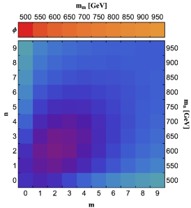
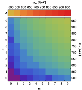
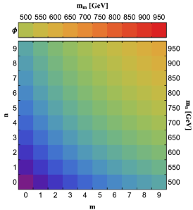
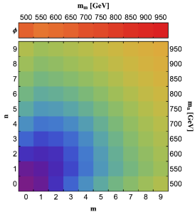
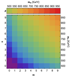
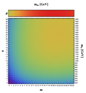
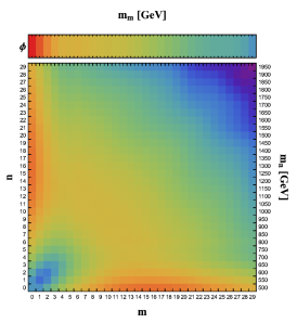
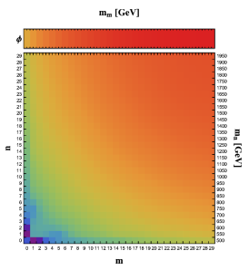
Figure 12: Production cross-sections before and after cuts for the processes $pp\rightarrow\phi\chi_{m}$ and $pp\rightarrow\chi_{m}\bar{\chi}_{n}$, calculated for the three benchmarks defined in Table 1 at the $\sqrt{s}=13$ TeV LHC.  The left column shows the cross-sections for these processes before any cuts are applied, while the center and right columns show the corresponding cross-sections after the application of the event-selection criteria associated with the monojet and multi-jet analyses described in the text, respectively. The results displayed in the top, middle, and bottom rows of the figure correspond to Benchmarks A, B, and C, respectively. The bar at the top of each panel shows the individual cross-sections $\sigma(pp\rightarrow\phi\chi_{m})$ for different values of the index $m$, while the density plot below it shows the cross-sections $\sigma(pp\rightarrow\chi_{m}\bar{\chi}_{n})$ for different values of the indices $m$ and $n$. We emphasize that a different color scheme is used in each column, owing to the significant difference in the overall scale of the cross-sections before and after cuts are applied.

By contrast, it turns out that the search strategies which are particularly relevant for probing the parameter space of our model are those commonly adopted in searches for supersymmetry in the multi-jet $+~{}{\hskip 2.56064pt/\hskip-6.544ptE_{T}}$ channel. In searches of this sort, signal events are selected primarily on the basis of $N_{\mathrm{jet}}$ and ${\hskip 2.56064pt/\hskip-6.544ptE_{T}}$. The leading constraints on our model from such searches are currently those from LHC $\sqrt{s}=13$ TeV searches by the ATLAS Collaboration Aaboud:2017hdf with $36.1\mathrm{~{}fb}^{-1}$ of integrated luminosity and those by the CMS Collaboration Sirunyan:2017cwe with $35.9~{}\mathrm{~{}fb}^{-1}$ of integrated luminosity. The ATLAS search turns out to be the more relevant of the two for constraining our example model, primarily because the CMS analysis includes a sizable ${\hskip 2.56064pt/\hskip-6.544ptE_{T}}$ cut. This leads to a significant reduction in statistics for our signal process.

For this reason, we assess the constraints on our model from the multi-jet channel by modeling our triggering requirements and event-selection criteria after those employed in Ref. Aaboud:2017hdf . In particular, we adopt the same triggering criteria that we used in constructing the detector-level $N_{\mathrm{jet}}$, ${\hskip 2.56064pt/\hskip-6.544ptE_{T}}$, and $H_{T}$ distributions in Sect. IV. In addition, primarily in order to reduce the SM multi-jet background, we impose the ${\hskip 2.56064pt/\hskip-6.544ptE_{T}}$ cut

$$\frac{{\hskip 2.56064pt/\hskip-6.544ptE_{T}}}{\sqrt{H_{T}}}~{}>~{}5~{}\mathrm{GeV}^{1/2}~{}.$$ (20)

Following Ref. Aaboud:2017hdf , we include only the three-momenta of jets with pseudorapidities in the range $|\eta_{j}|<4.5$ when calculating ${\hskip 2.56064pt/\hskip-6.544ptE_{T}}$ for a given event; likewise, we include only those jets with $p_{T_{j}}>40$ GeV and $|\eta_{j}|<2.8$ within the scalar sum in Eq. (19) when calculating $H_{T}$. Finally, we impose a cut on the total number of jets in the event which exceed a given $p_{T_{j}}$ threshold. More specifically, we define $N_{\mathrm{jet}}^{50}$ to be the number of jets with $p_{T_{j}}>50$ GeV in a given event and $N_{\mathrm{jet}}^{80}$ to be the number of jets with $p_{T_{j}}>80$ GeV.  We then perform an inclusive search involving a number of different signal regions defined by different combinations of the threshold cuts $N_{\mathrm{jet}}^{50}\geq\{8,9,10,11\}$ and $N_{\mathrm{jet}}^{80}\geq\{7,8,9\}$. For each channel, we impose the corresponding constraint on the parameter space of our example model by comparing the number of signal events $N_{s}$ after cuts with the 95% C.L. upper limit on $N_{s}$ in Ref. Aaboud:2017hdf . We emphasize that these signal regions are equivalent to those adopted in Ref. Aaboud:2017hdf for searches in the “heavy-flavor channel” with $N_{b-\mathrm{tag}}\geq 0$ — i.e., with no additional $b$-tagging requirement imposed. By contrast, searches in the “jet-mass channel,” which are particularly suited for probing new-physics scenarios involving highly-boosted massive particles which give rise to large-radius jets, are less constraining within our parameter-space region of interest. Highly-boosted $\phi$ or $\chi_{n}$ particles are not produced at any significant rate within this region, and the requirement that large-radius jets with jet masses above a few hundred GeV be present leads to a significant reduction in signal events.

While the most striking signals to which our example model gives rise would be detected in the multi-jet channel, this model can also give rise to observable signals in other channels relevant for new-physics searches. We must therefore ensure that our model is consistent with the results of existing searches in these channels within our parameter-space region of interest. For example, diagrams of the sort depicted in Fig. 4 contribute to the event rate in the monojet $+~{}{\hskip 2.56064pt/\hskip-6.544ptE_{T}}$ channel, as do diagrams similar to that shown in Fig. 4 in which an additional quark or gluon is produced as initial-state radiation or radiated off the internal $\phi$ line. Such diagrams clearly contribute to the event rate in the monojet $+~{}{\hskip 2.56064pt/\hskip-6.544ptE_{T}}$ channel whenever the ensemble constituents $\chi_{m}$ and $\overline{\chi}_{n}$ in the final state are both stable on collider timescales and therefore appear as ${\hskip 2.56064pt/\hskip-6.544ptE_{T}}$ within a collider detector. Searches in this channel play an important role in constraining single-particle dark-sector models with a similar mediator coupling structure TChannelMonojet , and thus can be anticipated to play an an important role in constraining the parameter space of our model as well.

Moreover, diagrams of this sort in which $\chi_{m}$ and/or $\overline{\chi}_{n}$ decay within the detector can also potentially contribute to the nominal signal-event rate in the monojet $+~{}{\hskip 2.56064pt/\hskip-6.544ptE_{T}}$ channel. This is because the event-selection criteria adopted in searches in this channel typically permit a small number of additional hadronic jets to be present in the final state. Thus, in assessing the monojet constraints on our example model, we must account for events in which the number of jets collectively produced by the decays of $\chi_{m}$ and/or $\overline{\chi}_{n}$ is sufficiently small that these event-selection criteria are satisfied.

The most stringent constraints on our model from searches in the monojet $+~{}{\hskip 2.56064pt/\hskip-6.544ptE_{T}}$ channel are those obtained by the ATLAS Collaboration with $36.1\ \mathrm{fb}^{-1}$ of integrated luminosity at the $\sqrt{s}=13$ TeV LHC ATLASMonojet . In assessing the constraints on our example model from searches in the monojet $+{\hskip 2.56064pt/\hskip-6.544ptE_{T}}$ channel, we model our triggering requirements and event-selection criteria after those employed in Ref. ATLASMonojet . In particular, we select events in which ${\hskip 2.56064pt/\hskip-6.544ptE_{T}}>250$ GeV and in which the leading jet has $p_{T_{j}}>250$ GeV and $|\eta_{j}|<2.4$. In addition, we require that there exist no more than four jets in the event with $p_{T_{j}}>30$ GeV and $|\eta_{j}|<2.8$. We also impose the criterion $\Delta\phi({\hskip 2.56064pt/\hskip-6.544pt\vec{p}_{T}},\vec{p}_{j})>0.4$, where $\Delta\phi({\hskip 2.56064pt/\hskip-6.544pt\vec{p}_{T}},\vec{p}_{j})$ is the difference in azimuthal angle between the missing-transverse-momentum vector ${\hskip 2.56064pt/\hskip-6.544pt\vec{p}_{T}}$ and the three-momentum vector $\vec{p}_{j}$ of any reconstructed jet in the event.

Finally, we note that while the most striking multi-jet signatures which arise in our model are those involving large jet multiplicities, channels involving a more modest number of jets and ${\hskip 2.56064pt/\hskip-6.544ptE_{T}}$ can also potentially be relevant for constraining the parameter space of our model. Indeed, Fig. 10 indicates that a significant number of events with 5–6 jets can be produced even within regions of parameter space where the peak on the $N_{\mathrm{jet}}$ distribution is much higher. The leading constraints of this sort turn out to be those from an ATLAS search Aaboud:2017vwy for squarks and gluinos in events involving 2–6 hadronic jets and substantial ${\hskip 2.56064pt/\hskip-6.544ptE_{T}}$. However, as we shall see, constraints from such moderate-jet-multiplicity searches turn out to be subleading compared to those from the monojet $+~{}{\hskip 2.56064pt/\hskip-6.544ptE_{T}}$ and multi-jet $+~{}{\hskip 2.56064pt/\hskip-6.544ptE_{T}}$ searches discussed above.

	Before Cuts			After Monojet Cuts			After Multi-Jet Cuts
Benchmark	$\sigma_{\chi\chi}$ (fb)	$\sigma_{\phi\chi}$ (fb)	$\sigma_{\phi\phi}$ (fb)	$\epsilon_{1}\sigma_{\chi\chi}$ (fb)	$\epsilon_{1}\sigma_{\phi\chi}$ (fb)	$\epsilon_{1}\sigma_{\phi\phi}$ (fb)	$\epsilon_{N}\sigma_{\chi\chi}$ (fb)	$\epsilon_{N}\sigma_{\phi\chi}$ (fb)	$\epsilon_{N}\sigma_{\phi\phi}$ (fb)
A	0.28	4.19	4.29	0.015	0.41	0.32	$7.6\times 10^{-4}$	0.058	0.12
B	9.72	23.9	4.29	0.32	0.77	0.10	0.10	0.87	0.24
C	3.06	0.92	$9.1\times 10^{-3}$	0.065	$6.0\times 10^{-3}$	$1.4\times 10^{-5}$	0.62	0.34	$4.6\times 10^{-3}$
LHC Limit				531			7.2

Table 2: The inclusive cross-sections $\sigma_{\chi\chi}$, $\sigma_{\phi\chi}$, and $\sigma_{\phi\phi}$ defined in Eq. (15) at the $\sqrt{s}=13$ TeV LHC, as well as the corresponding cross-sections after the application of the event-selection associated with the monojet search and multi-jet searches described in the text. Also shown are the corresponding experimental upper limits on the overall production cross-section after cuts for both of these monojet and multi-jet searches.

In Fig. 12, we present our results for the individual cross-sections $\sigma(pp\rightarrow\phi\chi_{m})$ for different values of the index $m$ and the individual cross-sections $\sigma(pp\rightarrow\chi_{m}\bar{\chi}_{n})$ for different combinations of the indices $m$ and $n$ for the three benchmarks defined in Table 1 at the $\sqrt{s}=13$ TeV LHC.  The results in the top, middle, and bottom rows of the figure correspond to Benchmarks A, B, and C, respectively. The left panel in each row of the figure shows these cross-sections before any cuts are applied, while the center and right panels in the same row show the corresponding cross-sections after the application of the event-selection criteria associated with searches in the monojet and multi-jet channels, respectively. More specifically, the monojet results shown here correspond the event-selection criteria associated with Signal Region IM1 of Ref. ATLASMonojet with ${\hskip 2.56064pt/\hskip-6.544ptE_{T}}>250$ GeV, while the multi-jet results correspond to the Signal Region $N_{\mathrm{jet}}^{50}\geq 8$ of Ref. Aaboud:2017hdf with $N_{b-\mathrm{tag}}\geq 0$.

In interpreting the results shown in Fig. 12, we begin by observing that for Benchmark A, the individual cross-sections $\sigma(pp\rightarrow\phi\chi_{m})$ before cuts are larger for heavier $\chi_{m}$, due primarily to the fact that $\gamma$ is positive. This remains true even after the application of the multi-jet cuts, as shown in the top right panel of the figure. By contrast, after the monojet cuts are applied, $\sigma(pp\rightarrow\phi\chi_{0})$ is by far the largest of the $\sigma(pp\rightarrow\phi\chi_{m})$ for this benchmark. This is primarily a consequence of the upper limit on $N_{\mathrm{jet}}$ included among these cuts. Similar behavior is also apparent for this benchmark within the $\chi\chi$ channel. The results obtained for Benchmark B are qualitatively similar to those obtained for Benchmark A, except that the individual contributions $\sigma(pp\rightarrow\phi\chi_{m})$ and $\sigma(pp\rightarrow\chi_{m}\bar{\chi}_{n})$ involving heavier $\chi_{m}$ contribute more significantly even after the monojet cuts. This is primarily a reflection of the fact that $\gamma$ is larger for Benchmark B than it is for Benchmark A.  For Benchmark C, the larger value of $m_{\phi}$ implies that the number of states in the ensemble is significantly larger than it is for the other two benchmarks. This larger value of $N$ notwithstanding, the results for this benchmark are also qualitatively similar to those obtained for Benchmark A.  The most salient difference between the results obtained for these two benchmarks is the significant decrease in $\sigma(pp\rightarrow\chi_{m}\bar{\chi}_{n})$ when both $m$ and $n$ become large. This is simply a reflection of the fact that both of the ensemble constituents are quite heavy in this regime.

The total production cross-sections $\sigma_{\chi\chi}$, $\sigma_{\phi\chi}$, and $\sigma_{\phi\phi}$ obtained by summing the contributions from all relevant individual production processes are provided in Table 2. The cross-sections before the application of any cuts are provided, as well as the corresponding cross-sections obtained after the application of our monojet and multi-jet cuts. Once again, the monojet results correspond the event-selection criteria associated with Signal Region IM1 of Ref. ATLASMonojet with ${\hskip 2.56064pt/\hskip-6.544ptE_{T}}>250$ GeV, while the multi-jet results correspond to the Signal Region $N_{\mathrm{jet}}^{50}\geq 8$ of Ref. Aaboud:2017hdf with $N_{b-\mathrm{tag}}\geq 0$. Current limits on the overall production cross-section from LHC monojet and multi-jet searches are also included in the bottom row of the figure for purposes of comparison. For Benchmark A, we observe that $\sigma_{\phi\chi}$ and $\sigma_{\phi\phi}$ are approximately equal and both much larger than $\sigma_{\chi\chi}$ before cuts. However, $\epsilon_{1}\sigma_{\phi\chi}$ is slightly larger than $\epsilon_{1}\sigma_{\phi\phi}$ after the monojet cuts are applied, and $\epsilon_{N}\sigma_{\phi\phi}$ dominates the overall production rate after the application of the multi-jet cuts. For Benchmark B, $\sigma_{\phi\chi}$ dominates the total production cross-section both before and after each set of cuts is applied. Likewise, for Benchmark C, $\sigma_{\chi\chi}$ dominates both before and after cuts, though the contribution from $\epsilon_{N}\sigma_{\phi\chi}$ after the application of the multi-jet cuts, while subleading in comparison with $\epsilon_{N}\sigma_{\chi\chi}$, is non-negligible.

More importantly, however, we observe that all three of these benchmark points are consistent with LHC limits from both monojet and multi-jet searches, despite the fact that a different production process provides the leading contribution to the overall event rate in the multi-jet channel in each case. Thus, we see that a variety of qualitatively different scenarios which give rise to mediator-induced decay cascades can be consistent with current constraints and therefore potentially within the discovery reach of future collider searches.

VI Surveying the Parameter Space

Having gained from our benchmark studies a sense of the range of phenomenological possibilities which can arise within our model, we now expand our analysis by performing a more systematic survey of the phenomenological possibilities that arise across the full parameter space of this model. The purpose of this survey is not only to assess the impact of current experimental constraints, but also to determine which of the production processes discussed in Sect. II dominates the event rate within different regions. In performing this survey, we shall vary the mediator mass $m_{\phi}$ and the scaling exponent $\gamma$ which determines how the mediator interacts with the fields of the dark sector while holding fixed the parameters $m_{0}=500$ GeV, $\Delta m=50$ GeV, and $\delta=1$ which characterize the internal structure of the dark sector itself. For simplicity, and in order to maintain consistency with the constraints outlined in Sect. III across the $(m_{\phi},\gamma)$-plane, we fix $c_{0}=0.1$. More specifically, we sample $m_{\phi}$ and $\gamma$ at a variety of discrete values within the ranges $0.6\mbox{~{}TeV}\leq m_{\phi}\leq 2.5\mbox{~{}TeV}$ and $0\leq\gamma\leq 3.5$. For each such combination of $m_{\phi}$ and $\gamma$, we then evaluate the aggregate cross-sections $\sigma_{\phi\phi}$, $\sigma_{\phi\chi}$, and $\sigma_{\chi\chi}$ according to the event-generation and event-selection procedures outlined in Sect. IV.  In addition, in order to provide a measure of the fraction of events associated with any particular combination of these parameters have truly large jet multiplicities, we also define the parameter $N_{\mathrm{jet}}^{10\%}$, which represents the maximum value of $N_{\mathrm{jet}}$ for which at least 10% of the events in a given data sample have $N_{\mathrm{jet}}\geq N_{\mathrm{jet}}^{10\%}$.

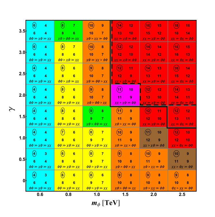
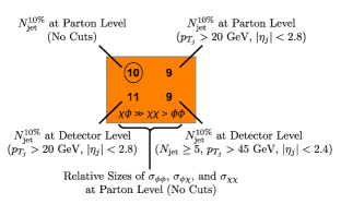
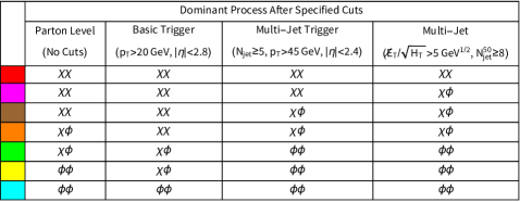
Figure 13: Summary of the collider-phenomenology consequences of the mediator-induced decay cascades within our model, plotted for discrete points within the $(m_{\phi},\gamma)$ plane with $m_{0}=500$ GeV, $\Delta m=50$ GeV, $\delta=1$, and $c_{0}=0.1$ held fixed. Each box within the figure corresponds to a particular combination of $m_{\phi}$ and $\gamma$. The four numbers displayed in each box indicate the values of $N_{\mathrm{jet}}^{10\%}$ obtained after the application of the cuts specified in the key at the bottom left. The text at the bottom of each box indicates the relative sizes of the cross-sections $\sigma_{\phi\phi}$, $\sigma_{\phi\chi}$, and $\sigma_{\chi\chi}$ at the parton level, before cuts. The color of each box indicates which production process dominates the overall cross-section for decay-cascade events after the application of the different sets of event-selection criteria described in the legend at the bottom right. As discussed in the text, the thick, black solid contour represents the bound from multi-jet searches, while the thick, black dashed contour represents the corresponding bound from moderate-jet-multiplicity searches. The regions above and to the right of these contours are excluded.

The results of this parameter-space survey are shown in Fig. 13. Each individual box within the figure corresponds to a particular combination of $m_{\phi}$ and $\gamma$. The four numbers displayed within each box indicate the value of $N_{\mathrm{jet}}^{10\%}$ at four different stages of our analysis, as indicated in the key at the bottom left of the figure. The number enclosed within a black circle in the upper left of each box indicates the value of $N_{\mathrm{jet}}^{10\%}$ at the parton level with no additional cuts, while the number in the upper right indicates the corresponding value obtained at the parton level with the basic trigger cuts $p_{T_{j}}>20$ GeV and $|\eta_{j}|<2.8$ applied. Similarly, the number in the lower left indicates the value of $N_{\mathrm{jet}}^{10\%}$ obtained at detector level with the same basic trigger applied, while the number in the lower right indicates the value of $N_{\mathrm{jet}}^{10\%}$ obtained after the application of the multi-jet trigger cuts $N_{\mathrm{jet}}\geq 5$, $p_{T_{j}}>45$ GeV, and $|\eta_{j}|<2.4$. The text at the bottom of each box indicates the relative size of the cross-sections $\sigma_{\phi\phi}$, $\sigma_{\phi\chi}$, and $\sigma_{\chi\chi}$ at the parton level, before the application of any cuts. The color of each box indicates which production process dominates the overall cross-section for mediator-induced decay-cascade events after the application of the different sets of event-selection criteria described in the legend at the bottom right of the figure. We note that the event-selection criteria associated with the results shown in the “Multi-Jet” column of the legend include not only the cuts explicitly listed in the heading of that column, but also the cuts associated with the multi-jet trigger.

Comparing the $N_{\mathrm{jet}}^{10\%}$ values appearing in the upper left and upper right corners of a given box provides a sense of how rudimentary cuts associated with jet-energy thresholds and detector geometry affect the $N_{\mathrm{jet}}$ distribution, while comparing the values shown in the upper left and lower left corners provides information about the effects of ISR, FSR, and parton-showering. We observe that throughout the region of the $(m_{\phi},\gamma)$-plane shown in the figure, geometric and jet-energy-threshold effects do not have a significant impact on $N_{\mathrm{jet}}^{10\%}$. We also observe that while the effects of ISR, FSR, and parton-showering are less uniform across the $(m_{\phi},\gamma)$-plane, leading to an increase in $N_{\mathrm{jet}}^{10\%}$ in some regions and a reduction in others, the overall impact on these effects is not particularly dramatic within any region of the plane. The reduction in $N_{\mathrm{jet}}^{10\%}$ which results from the application of the multi-jet cuts is typically more pronounced. However, the overall message is that whenever mediator-induced decay chains tend to generate a significant number of “jets” at the parton level, this typically translates into a significant population of events with large jet multiplicities at the detector level as well.

In addition to information about jet multiplicities, Fig. 13 also provides information about how the bounds discussed in Sect. V constrain the parameter space of our model. In particular, the solid black jagged line separates the points within out parameter-space scan which satisfy the bound from the multi-jet search limits derived in Ref. Aaboud:2017hdf from the points which do not. Similarly, the dashed black jagged line separates the points within our parameter-space scan which satisfy the bound from the moderate-jet-multiplicity search limits derived in Ref. Aaboud:2017vwy from the points which do not. The regions above and to the right of each contour are excluded by the corresponding constraint. By contrast, we find that the constraints from the monojet search limits derived in Ref. ATLASMonojet do not exclude any of the parameter space shown.

We see from Fig. 13 that the region of parameter space in which $m_{\phi}$ and $\gamma$ are both large — and in which processes of the form $pp\rightarrow\chi_{m}\bar{\chi}_{n}$ dominate the event rate — is the region most severely impacted by the constraints from multi-jet searches (which supersede the moderate-jet-multiplicity searches throughout the region shown). Nevertheless, we observe that regions of parameter space remain within which such processes dominate the event rate both before and after cuts are applied, while at the same satisfying these constraints. While the values of $N_{\mathrm{jet}}^{10\%}$ are largest within this excluded region at all stages of our analysis, we note that there exists a substantial region of the allowed parameter space wherein $N_{\mathrm{jet}}^{10\%}\geq 8$ even after the application of the multi-jet cuts. This is the region within which $m_{\phi}$ is large, $\gamma$ is small, and processes of the form $pp\rightarrow\phi\chi_{n}$ dominate the overall event rate. By contrast, within regions of parameter space where $m_{\phi}$ is small, $N$ is likewise small and the number of individual processes of the form $pp\rightarrow\phi\chi_{n}$ or $pp\rightarrow\chi_{m}\bar{\chi}_{n}$ which contribute to the overall event rate is comparatively small. As a result, $pp\rightarrow\phi^{\dagger}\phi$ tends to dominate the event rate in this region and $N_{\mathrm{jet}}^{10\%}$ tends not to be terribly high in comparison with the results obtained for larger values of $m_{\phi}$. That said, we note that reasonably large jet multiplicities can still arise within this region, especially for cases in which $\gamma$ is large.

The results shown in Fig. 13 demonstrate that while existing LHC searches impose non-trivial constraints on the parameter space of our model, there nevertheless exists a substantial region of that parameter space within which extended mediator-induced decay cascades arise without violating these constraints. The prospects for probing these regions of parameter space at future colliders — or through use of alternative search strategies at the LHC — will be discussed in Sect. VIII.

VII Implications Beyond Colliders: A Consistency Check

Our primary aim in this paper has been to investigate the general properties of mediator-induced decay chains and the multi-jet signatures to which such decay chains can give rise at colliders. Indeed the model which we introduced in Sect. II was chosen simply for purposes of illustration, and similar signatures can arise across a broad class of new-physics scenarios in which multiple dark-sector states interact with the fields of the SM through a common mediator. For this reason, we have thus far focused exclusively on collider considerations in placing constraints on this model.

That said, one might wonder whether other constraints — such as those from flavor physics or cosmology — generically exclude new-physics scenarios which are capable of yielding observable jet-cascade signatures of this sort at the LHC or at future colliders. Thus, in this section, we demonstrate that our illustrative model is indeed consistent with these additional constraints. In so doing, we furnish a proof of concept that new-physics scenarios which would give rise to multi-jet collider signals of mediator-induced decay chains at the LHC or at future colliders can indeed be compatible with all applicable constraints.

VII.1 Flavor-Physics Considerations

The first set of constraints we consider are those from flavor physics. As noted in Sect. II, our illustrative model can potentially give rise to FCNCs, which are tightly constrained by data. However, there exist standard methods through which constraints on FCNCs can easily be satisfied in models of this type.

Most such methods are rooted in the principle of minimal flavor violation MFV — i.e., the principle that there exists a unique source for the breaking of the $U(3)_{Q}\times U(3)_{u}\times U(3)_{d}$ flavor symmetry that would exist in the quark sector of the SM in the absence of Yukawa couplings. Indeed, an approach along these lines was employed in Ref. TChannelHaipeng within the context of a model involving a coupling structure identical to that in Eq. (4), but involving only one dark-sector particle species. In this approach, one posits that $\phi$ transforms as a triplet under the $U(3)_{u}$ symmetry which acts on the right-handed up-type quarks. The simplest way to ensure that the mass term for $\phi$ accords with the principle of minimal flavor violation is to posit that the mass matrix for the component fields in $\phi$ is proportional to the identity matrix in flavor space. In this case, this mass matrix remains invariant under arbitrary $U(3)_{u}$ transformations and is therefore diagonal in the basis in which the quark-mass matrix is likewise diagonal. The three physical fields $\phi_{u}$, $\phi_{c}$, and $\phi_{t}$ within the $\phi$ multiplet are degenerate in mass, with $m_{\phi_{u}}=m_{\phi_{d}}=m_{\phi_{t}}$, and each couples at tree level exclusively to a single quark species. As a result, the leading contributions to FCNC processes that would otherwise arise as a consequence of Eq. (4) vanish, and all higher-order corrections are suppressed by powers of the small, off-diagonal elements in the Cabibbo-Kobayashi-Maskawa matrix. Thus, even for reasonably large values of $N$, such modifications render our model compatible with experimental constraints on FCNCs. Moreover, we emphasize that more complicated structures in which $m_{\phi_{u}}$, $m_{\phi_{c}}$, and $m_{\phi_{t}}$ are not degenerate can also be consistent with the principle of minimal flavor violation and a similar suppression to FCNCs.

The results we have explicitly derived in this paper, which pertain the case in which there exists a single mediator $\phi$ with a coupling structure such that $c_{0u}\neq 0$ and $c_{0q}=0$ for $q=\{c,t\}$, can also be viewed as pertaining to the regime in which a hierarchy $m_{\phi_{u}}\ll m_{\phi_{c}},m_{\phi_{t}}$ exists among the masses of these three mediator generations. However, it is also interesting to consider how these results are modified in the regime in which $m_{\phi_{u}}$, $m_{\phi_{c}}$, and $m_{\phi_{t}}$ are degenerate. We begin by considering the effect of introducing additional generations of mediator particles on the decay phenomenology of our model. In the regime in which $m_{\phi_{u}}=m_{\phi_{d}}=m_{\phi_{t}}$, the branching fractions $\mathrm{BR}_{\phi n}$ and $\mathrm{BR}_{n\ell}$ are the same as in the regime in which $m_{\phi_{u}}\ll m_{\phi_{c}},m_{\phi_{t}}$. Moreover, given that $m_{c}\ll\Delta m$ within our parameter-space region of interest, the total widths of $\phi_{u}$ and $\phi_{c}$ are approximately equal in the degenerate-mass regime and both approximately equal to the result for $\Gamma_{\phi}$ obtained in the hierarchical-mass regime. By contrast, the total width of each $\chi_{n}$ is effectively doubled, since contributions to each partial width $\Gamma_{n\ell}$ arise both from the process $\chi_{n}\rightarrow\bar{u}u\chi_{\ell}$, which involves a virtual $\phi_{u}$, and from the process $\chi_{n}\rightarrow\bar{c}c\chi_{\ell}$, which involves a virtual $\phi_{c}$. (Contributions to $\Gamma_{n\ell}$ from $\chi_{n}\rightarrow\bar{t}t\chi_{\ell}$ are suppressed in comparison with these other processes, due to the mass of the top quark.) This modification has the effect of relaxing the lower limit on $c_{0}$ shown in Fig. 9, thereby opening up additional regions of model-parameter space.

Introducing additional generations of mediator particles also has an effect on the cross-sections for the various production processes which give rise to mediator-induced decay chains in our model. The cross-sections for the production processes $pp\rightarrow\chi_{m}\overline{\chi}_{n}$ and $pp\rightarrow\phi\chi_{n}$ will not change significantly, given that parton-distribution function for $u$ within the proton is much larger than that for $c$ at all relevant momentum fractions and energy scales. By contrast, in the degenerate-mass regime, the combined cross-section for $pp\rightarrow\phi_{u}\phi_{u}$ and $pp\rightarrow\phi_{c}\phi_{c}$ — processes which proceed primarily via gluon fusion and give rise to effectively indistinguishable decay cascades — is approximately double the cross-section for $pp\rightarrow\phi_{u}\phi_{u}$ in the hierarchical-mass regime. (The process $pp\rightarrow\phi_{t}\phi_{t}$ leads to entirely different event topologies necessarily involving at least one top-quark pair, and therefore must be considered separately.) However, even when this doubling is taken into account, we find that the boundary between the allowed and excluded regions of parameter space in Fig. 13 does not change. Thus, in going from the hierarchical-mass regime to the degenerate-mass regime, the main conclusions of Sect. VI are unchanged.

VII.2 Cosmological Considerations

The second set of considerations we consider are those from early-universe cosmology. Since we are assuming that all $\chi_{n}$ with $n>0$ decay promptly within a collider detector, these particles decay far too early within the history of the universe to have any appreciable effect on cosmological observables. However, no contribution to the width of $\chi_{0}$ arises as a consequence of Eq. (4), and we have thus far made no assumptions about the lifetime $\tau_{0}$ of this particle, other than that it is stable on collider timescales. Indeed, it is possible that $\chi_{0}$ decays as a result of additional, highly suppressed interactions on far longer timescales. If $\tau_{0}$ is sufficiently long-lived, a cosmological population of this lightest ensemble constituent could have observable consequences for early-universe cosmology or particle astrophysics. There are essentially two relevant regimes we must consider, based on the relationship between $\tau_{0}$ and the present age of the universe. We shall address these two possibilities in turn.

The first possibility is that $\tau_{0}$ far exceeds collider timescales, but is nevertheless significantly shorter than the observable age of the universe. In this case, we simply stipulate that $\tau_{0}$ is sufficiently short that constraints from Big-Bang nucleosynthesis CyburtBBN ; JedamzikBBN1 ; KawasakiBBN1 ; JedamzikBBN2 ; KawasakiBBN2 , spectral distortions to the cosmic microwave background HuSilk1 ; HuSilk2 ; Chluba1 ; Chluba2 , modifications of the ionization history of the universe SlatyerDarkAges ; SlatyerCMB ; PoulinIonization , etc., are satisfied. Indeed, this is the simplest way in which the illustrative model we introduced in Sect. II can be rendered consistent with cosmological constraints. Moreover, we note that for certain values of $\tau_{0}$ within this regime, an unstable $\chi_{0}$ could potentially also give rise to signals at a dedicated surface detector like MATHUSLA MATHUSLA ; MATHUSLAWhitePaper .

The second possibility is that $\chi_{0}$ is cosmologically — and perhaps even absolutely — stable. In this case, we must ensure that cosmological and astrophysical constraints on whatever relic population of $\chi_{0}$ particles is generated during the early universe are satisfied within the region of model-parameter space wherein multi-jet signatures of mediator-induced decay chains would be accessible at the LHC or at future colliders. Moreover, it is also interesting to consider whether a relic population of $\chi_{0}$ particles could account for the present-day abundance of dark matter in our universe within this same parameter-space regime. In order for this possibility to be realized, $\chi_{0}$ must not only acquire a present-day cosmological abundance $\Omega_{0}$ similar to the dark-matter abundance $\Omega_{\mathrm{CDM}}\approx 0.26$ inferred from Planck data Planck , but also satisfy constraints from direct- and indirect-detection experiments.

In principle, there are two contributions to $\Omega_{0}$ which one must consider within the context of our model. First, since the scattering processes that follow from Eq. (4) maintain thermal equilibrium between $\chi_{0}$ and the visible-sector particles in the radiation bath at high temperatures $T\gg m_{0}$, this lightest ensemble constituent generically acquires a contribution to its abundance from thermal freeze-out. Second, the late decays of long-lived $\chi_{n}$ with $n>0$ can give rise to an additional, non-thermal contribution to this abundance. However, assuming that $\chi_{0}$ freezes out during a radiation-dominated epoch, the time $t_{\rm fr}$ at which freeze-out effectively occurs is given by

$$t_{\rm fr}~{}\approx~{}\sqrt{\frac{45}{2\pi^{2}}}\,g^{-1/2}_{\ast}(T_{\rm fr})\frac{M_{P}}{T_{\rm fr}^{2}}~{},$$ (21)

where $M_{P}$ is the reduced Planck mass, where $T_{\rm fr}\approx m_{0}/20$ is the freeze-out temperature, and $g_{\ast}(T_{\rm fr})$ is the number of effectively massless degrees of freedom in the radiation bath at this temperature. Comparing $t_{\rm fr}$ to the the lifetimes $\tau_{n}$ for all of the $\chi_{n}$ with $n>0$ within our parameter-space region of interest, we typically find that $\tau_{n}\ll t_{\rm fr}$ for all of these heavier $\chi_{n}$. Any $\chi_{0}$ particles produced in the early universe via the decays of these heavier $\chi_{n}$ therefore attain thermal equilibrium with the radiation bath prior to freeze-out. Moreover, since all of the $\chi_{n}$ with $n>0$ effectively decay away well before $\chi_{0}$ freezes out, the effect of coannihilation processes of the form $\overline{\chi}_{n}\chi_{m}\rightarrow\bar{q}q$ on $\Omega_{0}$ is also negligible. Thus, within our parameter-space region of interest, the only relevant contribution to $\Omega_{0}$ is that from thermal freeze-out, where the annililation rate of $\chi_{0}$ is governed solely by $t$-channel processes of the form $\overline{\chi}_{0}\chi_{0}\rightarrow\bar{q}q$ involving a virtual $\phi$.

Taking these considerations into account, we evaluate $\Omega_{0}$ numerically using the MadDM MadDM code package for the same parameter choices $m_{0}=500$ GeV and $c_{0}=0.1$ as in Fig. 13 and a sampling of mediator masses within the range $0.6\mathrm{~{}TeV}\leq m_{\phi}\leq 2.5\mathrm{~{}TeV}$. For all values of $m_{\phi}$ within this range, we find that $\Omega_{0}$ exceeds $\Omega_{\mathrm{CDM}}$ — at least within the context of the standard cosmology. However, within the context of a modified cosmology — for example, one in which the abundance of $\chi_{0}$ is diluted at late times due to an injection of entropy from late-decaying particles after freeze-out has occurred GelminiGondolo — the abundance of such a particle can easily be reduced to an acceptable level. Within such a modified cosmology, then, a cosmologically stable $\chi_{0}$ can acquire an abundance $\Omega_{0}\approx\Omega_{\mathrm{CDM}}$ and constitute the majority of the dark matter.

Of course, in order for $\chi_{0}$ to account for a non-negligible fraction of $\Omega_{\mathrm{CDM}}$, constraints from direct- and indirect-detection experiments must also be satisfied. We begin by discussing the constraints from direct detection. The leading contribution to the event rate for elastic scattering between $\chi_{0}$ particles in the local dark-matter halo and the atomic nuclei in a dark-matter detector arises due to fundamental processes of the form $q\overline{\chi}_{0}\rightarrow q\overline{\chi}_{0}$ involving an $s$-channel mediator. Such processes yield both a spin-dependent and a spin-independent contribution to the event rate TChannelHaipeng . For the case we are considering here, in which $\chi_{0}$ is a Dirac fermion, the dominant contribution is from spin-independent scattering. We shall therefore focus on this spin-independent contribution in what follows. In doing so, we note that inelastic-scattering processes of the form $q\overline{\chi}_{0}\rightarrow q\overline{\chi}_{n}$ with $n>0$ are irrelevant for direct-detection phenomenology, given that $\Delta m\gg\mathcal{O}({\rm MeV})$ throughout our parameter-space region of interest.

The most stringent constraint on $\sigma^{\rm(SI)}$ for a dark-matter particle with this mass is the bound $\sigma^{\rm(SI)}<6.44\times 10^{-46}$ cm² set by the XENON1T experiment XENON1T . In order to assess whether this constraint can be satisfied within our parameter-space region of interest, we evaluate the spin-independent cross-section per nucleon $\sigma^{\rm(SI)}$ for the parameter choices used in Fig. 13 using the MadDM MadDM code package. We find that the spin-independent cross-section per nucleon decreases with increasing $m_{\phi}$ from $\sigma^{\rm(SI)}\approx 4.88\times 10^{-44}$ cm² for $m_{\phi}=0.6$ TeV to $\sigma^{\rm(SI)}\approx 4.86\times 10^{-47}$ cm² for $m_{\phi}=2.5$ TeV, and that the bound from XENON1T is satisfied for $m_{\phi}\gtrsim 1.5$ TeV.  Moreover, we note that for certain choices of $c_{0}$ and $m_{0}$ which differ only slightly from these benchmark values, even lower values of $m_{\phi}$ can be accommodated.

The leading indirect-detection constraints on a cosmologically stable population of $\chi_{0}$ particles are those derived from Fermi-LAT observations of dwarf spheroidal galaxies and other Milky-Way satellites Fermi2016 . In order to assess the implications of these constraints within our parameter-space region of interest, we compute the expected gamma-ray flux from $\overline{\chi}_{0}\chi_{0}\rightarrow\bar{q}q$ annihilation within the dark-matter halos of these Milky-Way satellites using the MadDM MadDM code package, which incorporates the $J$-factors derived in Ref. DwarfProfiles . For the same $m_{0}$ and $c_{0}$ as in Fig. 13 and a mediator mass of $m_{\phi}=600$ GeV, we find that the velocity-averaged annihilation cross-section is $\langle\sigma v\rangle\approx 2.25\times 10^{-29}$ cm³/s, which is well below the corresponding bound $\langle\sigma v\rangle\leq 2.30\times 10^{-25}$ cm³/s from Fermi-LAT data. Since increasing $m_{\phi}$ for the same $m_{0}$ further suppresses $\langle\sigma v\rangle$, we find that a cosmological population of $\chi_{0}$ with $\Omega_{0}\approx\Omega_{\mathrm{CDM}}$ is consistent with the Fermi-LAT data.

We therefore conclude that a cosmologically stable $\chi_{0}$ is a viable dark-matter candidate within our parameter-space region of interest. Indeed, the phenomenological consequences of such a particle do not conflict with bounds from direct- and indirect-detection data. Moreover, in the presence of a source of late entropy injection subsequent to thermal freeze-out, this lightest ensemble constituent can also acquire an appropriate abundance.

VIII Conclusions and Outlook

In this paper, we have investigated the collider phenomenology of scenarios in which multiple dark-sector particles with similar quantum numbers couple to the fields of the visible sector via a common massive mediator. In such scenarios, the mediator not only plays an important role in providing a portal through which the dark and visible sectors interact, but also necessarily gives rise to decay processes wherein heavier dark-sector particles decay to final states which include both lighter dark-sector particles and visible-sector fields. In cases in which these visible-sector fields are quarks or gluons, successive decays of this sort give rise to extended decay cascades involving large numbers of hadronic jets at hadron colliders. We have investigated the structure of these mediator-induced decay cascades and examined how existing LHC searches constrain the parameter spaces associated with such scenarios. We have also shown that there exist large regions of parameter space within which all applicable constraints from these searches are satisfied, but within which extended decay cascades of this sort develop and within which jet multiplicities are characteristically large. Thus, striking signatures of this sort could potentially manifest themselves at forthcoming LHC runs or at future colliders. Such signatures could therefore provide a way of probing the properties of the dark sector and the mediator through which it couples to the SM.

Many possible extensions of our analysis can be envisioned. For example, in this study, we have chosen to focus on the region of parameter space in which the number of jets with $p_{T}$ sufficient to satisfy the applicable jet-identification criteria is effectively maximized. Thus, we have chosen our model parameters such that $m_{N-1}<m_{\phi}$ and such that the lifetimes of all $\chi_{n}$ with $n>0$ are sufficiently short that these particles typically decay promptly within a collider detector. However, it would be interesting to examine the discovery prospects for our model within other regions of parameter space as well — regions within which extended mediator-induced decay cascades still arise, but within which the collider phenomenology nevertheless differs in salient ways.

One such alternative possibility arises in the regime in which $m_{N-1}\ll m_{\phi}$ In such cases, any ensemble constituent $\chi_{n}$ initially produced by the decay of an on-shell mediator $\phi$ is highly boosted. In this regime, particles produced by the subsequent decay of this $\chi_{n}$ will be collimated in the direction of its three-momentum vector. A similar situation can also in principle arise in situations in which significant mass gaps occur within the mass spectrum of $\chi_{n}$. Such possibilities are under investigation DDMboosted .

In this connection, we also note that while the results of existing LHC searches are effective in probing and constraining scenarios involving mediator-induced decay cascades, alternative search strategies may be even more efficient in resolving the particular kinds of multi-jet signals which arise in these scenarios from SM backgrounds. For example, a variety of jet-shape variables and other jet-substructure techniques could potentially provide a way of improving the discovery reach for signatures of these cascades when such highly boosted particles arise. Such techniques can also be advantageous in probing regions in which parton-level “jet” multiplicities $N_{\mathrm{jet}}$ are typically so large that multiple jets within the same event inevitably overlap in $(\eta,\phi)$-space. In such cases, a moderate jet multiplicity at the detector level might therefore belie a much higher value of $N_{\mathrm{jet}}$. The application of jet-substructure techniques will be especially relevant at future hadron colliders with CM energies significantly higher than that of the LHC.  However, since the substructure of jets arising from mediator-induced decay cascades differs from the substructure of the jets produced by the decays of the heavy SM particles $W^{\pm}$, $Z$, and $t$, alternative jet-shape variables and clustering algorithms may be required DDMboosted .

Several additional phenomenological possibilities also arise in the regime in which many of the $\chi_{n}$ are sufficiently long-lived that they do not tend to decay promptly within a collider detector. For example, any $\chi_{n}$ with a characteristic decay length in the range $\mathcal{O}(1\mathrm{~{}cm})\lesssim L_{n}\lesssim\mathcal{O}(10\mathrm{~{}m})$ will give rise to events in which the jet cascades associated with the decays of the more massive, promptly-decaying constituents in the ensemble are accompanied by one or more macroscopically displaced vertices. Moreover, depending on the choice of model parameters, it is possible that the final-state ensemble constituent $\chi_{m}$ produced at one of these displaced vertices might itself decay within the detector a macroscopic distance away, and so forth. This could lead to spectacular and completely novel signatures involving multiple displaced vertices arising from the same decay chain. An investigation into the prospects for realizing and detecting such signatures at the LHC and at future colliders is currently underway DDMDisplaced .

Furthermore, any $\chi_{n}$ with decay lengths $L_{n}\gtrsim\mathcal{O}(10\mathrm{~{}m})$ will manifest themselves as ${\hskip 2.56064pt/\hskip-6.544ptE_{T}}$ within a collider detector. Whenever additional $\chi_{n}$ with $n>0$ have decay lengths in this range, the decay chains precipitated by any of the production processes depicted in Figs. 4–4 effectively terminate not merely when a $\chi_{0}$ particle is produced, but whenever any of these ensemble constituents is produced. This has a salient impact on the resulting multi-jet phenomenology. For example, for the case of $pp\rightarrow\phi^{\dagger}\phi$ production discussed in detail in Sect. III, the probability $\mathcal{P}_{\phi}(S)$ for such a decay chain to involve a particular number of steps $S$ would differ from the result in Eq. (13). We also note that long-lived particles within these ensembles could also give rise to observable signals at a dedicated surface detector such as MATHUSLA MATHUSLAWhitePaper ; DDMMATHUSLA — signals which could then be correlated with large-jet-multiplicity signatures in the main LHC detectors.

In all cases, however, our main message is clear. If the dark sector contains multiple components with similar quantum numbers, and if this sector communicates with the visible sector through a mediator, then this mediator has the potential to induce extended decay cascades yielding large multiplicities of SM particles. Moreover, as we have demonstrated in this paper, scenarios of this sort can be consistent with existing constraints. Thus, the detection of the corresponding collider signatures of these scenarios remains a viable future possibility. Such signatures might therefore provide an important route for uncovering and probing not only the dark sector but also the mediator through which it couples to the SM.