Metallicity and absolute magnitude calibrations for F-G type main-sequence stars in the Gaia era

Abstract

In this study, photometric metallicity and absolute magnitude calibrations were derived using F-G spectral type main-sequence stars in the Solar neighbourhood with precise spectroscopic, photometric and Gaia astrometric data for UBV photometry. The sample consists of 504 main-sequence stars covering the temperature, surface gravity and colour index intervals $5300<T_{eff}<7300$ K, $\log g>4$ (cgs) and $0.3<(B-V)_{0}<0.8$ mag, respectively. Stars with relative trigonometric parallax errors $\sigma_{\pi}/\pi\leq 0.01$ were preferred from Gaia DR2 data for the estimation of their $M_{V}$ absolute magnitudes. In order to obtain calibrations, $(U-B)_{0}$ and $(B-V)_{0}$ colour indices of stars were preferred and a multi-variable second order equation was used. Calibrations are valid for main-sequence stars in the metallicity and absolute magnitude ranges $-2<{\rm[Fe/H]}<0.5$ dex and $2.5<M_{V}<6$ mag, respectively. The mean value and standard deviation of the differences between original and estimated values for the metal abundance and absolute magnitude are $\langle\Delta{\rm[Fe/H]}\rangle=0.00\pm 0.11$ dex and $\langle\Delta M_{V}\rangle=0.00\pm 0.22$ mag, respectively. In this work, it has been shown that more precise iron abundance and absolute magnitude values were obtained with the new calibrations, compared to previous calibrations in the literature.

Keywords stars: abundances, stars: metallicity calibration, stars: distance

1 Introduction

Stars with different luminosity, if they have precise photometric, spectroscopic and astrometric data, play an important role to understand the structure, formation and evolution of the Milky Way. Specifically, F and G type main-sequence stars are used in Galactic archaeology surveys as they are long-lived objects and they contain the chemical composition of the molecule cloud in which they formed. These stars are often considered in the study of metallicity gradients and age-metallicity relations in the Galaxy disc, as well as in testing the scenarios related to the formation of the Galaxy (Sales et al., 2009; Robin et al., 2014; Helmi et al., 2018).

Today, data with high resolution and high signal-to-noise ratio are preferred to investigate the chemical composition of stars. Spectroscopic and astrometric data from large spectroscopic surveys such as RAVE (Steinmetz et al., 2006), APOGEE (Allende Prieto et al., 2008), SEGUE (Yanny et al., 2009), GES (Gilmore et al., 2012), LAMOST (Zhao et al., 2012), GALAH (de Silva et al., 2015), BRAVA (Kunder et al., 2012) and Gaia (Gaia Collaboration et al., 2018) are more valuable ones. Thanks to such spectroscopic surveys, radial velocities of stars as well as atmospheric model parameters are calculated. The metallicity, which is one of these parameters, has an important role in the investigation of the chemical evolution of our Galaxy.

The metallicity of stars can be determined by spectral analysis as well as by using photometric methods. Metallicity obtained from spectral methods gives more accurate results for the stars in the Solar neighbourhood, although sensitivity in metallicity decreases as SNR becomes lower towards the fainter stars at large distances. On the other hand, fainter objects may have accurate photometric data since they can be observed at higher SNRs, i.e. Sloan Digital Sky Survey (SDSS, York et al., 2000). Thus, the atmospheric model parameters calculated from spectra of nearby stars can be combined with accurate photometric data to determine the metallicity of fainter stars.

The photometric metallicity estimation method has been used by many researchers since 1950s. Roman (1955) calculated the ultra-violet (UV) excess of about 600 F and G spectral type stars with weak metallic lines by marking them in the $U-B\times B-V$ two-colour diagram. The author found that UV excesses of the stars change in the range of 0 to 0.2 mag and the stars with the largest UV excesses have the largest space velocities. In the past, many researchers have explained the UV excess with the “blanketing model” (Schwarzschild et al., 1955; Sandage & Eggen, 1959; Wallerstein, 1962), in which the stars with the same metal abundance but different $B-V$ colours contain different UV excesses in the $U-B\times B-V$ two-colour diagram. Sandage (1969) introduced a guillotine factor to normalize UV excesses to the one for $(B-V)_{0}=0.6$ mag and then calculated the normalized values for different $B-V$ colours. Carney (1979) explained the normalized UV excesses of the main-sequence stars within 100 pc according to the iron abundance by a quadratic equation. Karaali et al. (2003a) considered 77 main-sequence stars covering colour and iron abundance intervals $0.37<(B-V)_{0}<1.07$ mag and $-2.70<{\rm[Fe/H]}<+0.26$ dex, respectively, and calculated their UV excesses to the iron abundance by a cubic equation. Karataş & Schuster (2006) described UV excesses of the F and G spectral type main-sequence stars in the Solar neighbourhood according to the iron abundance by a quadratic equation. Karaali et al. (2011) obtained a more accurate photometric metallicity calibration using 701 main-sequence stars covering colour index and iron abundance intervals $0.32<(B-V)_{0}<1.16$ mag and $-1.76<{\rm[Fe/H]}<+0.40$ dex, respectively, in the UBV photometric system. Furthermore, there are several studies on photometric metallicity calibration developed for different photometric systems (Walraven & Walraven, 1960; Strömgren, 1966; Cameron, 1985; Laird et al., 1988; Buser & Fenkart, 1990; Trefzger et al., 1995). The most recent photometric metallicity calibration in the UBV system is presented by Tunçel Güçtekin et al. (2016). In their last study, Tunçel Güçtekin et al. (2017) obtained a photometric metallicity calibration for the SDSS photometric system using the transformation formulae of Chonis & Gaskell (2008).

In the investigation of chemical evolution of the Milky Way, distances of stars as well as their iron abundance must be known. Distances of the stars in the vicinity of the Sun is calculated by trigonometric parallax method, while photometric parallax is preferred for the more distant stars. Using the ground-based trigonometric data of nearby stars, Laird et al. (1988) calibrated differences in absolute magnitudes ($\Delta M_{V}$) of the field stars and Hyades stars with the same colour index, according to their UV excesses ($\delta_{0.6}$) and $(B-V)_{0}$ colour index of the stars. Using similar procedure and Hipparcos data (ESA, 1997), Karaali et al. (2003b) and Karataş & Schuster (2006) developed absolute magnitude calibrations in the UBV photometric system. Karaali et al. (2005), who established the metallicity and absolute magnitude calibrations in UBV photometric system, have moved their calibrations to the SDSS system using new photometric transformation equations. Bilir et al. (2005) and Juric et al. (2008) adapted the photometric parallax method to the SDSS system and produced calibrations to estimate the distances of the main-sequence stars. Bilir et al. (2008, 2009) calibrated trigonometric parallaxes of the main-sequence stars in the re-reduced Hipparcos catalogue (van Leeuwen, 2007) to UBV, SDSS and 2MASS, and obtained absolute magnitude relations for the main-sequence stars in the range of A and M types, which are located in the Galactic disc. Tunçel Güçtekin et al. (2016, 2017) calibrated absolute magnitudes of 168 F-G dwarfs and the re-reduced Hipparcos parallaxes to UBV and SDSS photometric systems.

Thanks to Gaia satellite data, it is aimed to create a three-dimensional map of more than one billion objects in our Galaxy and beyond, and to investigate the origin and subsequent evolution of the Milky Way. Gaia DR2 release includes astrometric data for 1.7 billion sources observed in 22 months from the beginning of the Gaia mission (Gaia Collaboration et al., 2018). It covers a large magnitude range with significant uncertainties in the trigonometric parallaxes. For example, astrometric uncertainties of the stars with $G$ = 15, 17, 20 and 21 mag reach 0.04, 0.1, 0.7 and 2 mas in parallax, respectively. This shows that uncertainties increase towards fainter stars. It is important to examine stars in different populations for understanding the structure and evolution of our Galaxy. Therefore, we need accurate photometric parallax relations obtained with calibration of sensitive photometric data to the Gaia astrometric data. In this study, we obtain photometric metallicity and absolute magnitude calibrations using F and G spectral type main-sequence stars in the Solar neighbourhood. In this context, this study can sort of be a supplementary work for Gaia DR2.

Even if distances of 1.3 billion objects can be calculated from trigonometric parallax data in Gaia DR2, uncertainties in measurements reduce the sensitivity in distances. In particular, this prevents researchers investigating star fields up to faint limiting apparent magnitudes to obtain reliable Galactic model parameters or Galactic metallicity gradients. Combining precise spectroscopic, astrometric and photometric data, metal abundance and absolute magnitude calibrations to be produced for large area photometric sky surveys, i.e. SDSS, Panoramic Survey Telescope and Rapid Response System (Pan-STARRS) etc., will make a significant contribution to the more sensitive metal abundance and distance calculations of faint stars. The accuracy of the absolute magnitude calibration could be compared with the expected Gaia trigonometric parallax accuracy at the end of the mission to show that the calibration could be useful in a few years. The same for metallicity which will be provided by Gaia probably in 2021.

This work provides metallicity and absolute magnitude calibrations for investigation of not only nearby stars but also distant stars in detail. It is organized as follows: Section 2 presents the data used in the calibrations. Section 3 describes the methods for calibrations. Section 4 contains a summary and discussion.

2 Data

In order to obtain precise metallicity and absolute magnitude calibrations, we prioritized the stars that have sensitive spectroscopic, astrometric and photometric data in the recent studies. In this context, we used the spectroscopic data from 12 studies (Boesgaard et al., 2011; Nissen & Schuster, 2011; Ishigaki et al., 2012; Mishenina et al., 2013; Molenda-Zakowicz et al., 2013; Bensby et al., 2014; da Silva et al., 2015; Sitnova et al., 2015; Brewer et al., 2016; Maldonado & Villaver, 2016; Luck, 2017; Delgado Mena et al., 2017). Information about the spectroscopic data used in this study is given in Table 1. We selected 5756 stars whose atmospheric model parameters ($T_{eff}$, $\log g$ and [Fe/H]) were derived in these studies. We took into account effective temperature ($T_{eff}$), surface gravity ($\log g$) and colour index $(B-V)$ given for a large spectral range of main-sequence stars. In the selection of F-G type main-sequence stars, we constrained the effective temperatures ($5300<T_{eff}<7300$ K) and surface gravities ($\log g\geq 4$ cgs) and composed 3413 stars in total. These limits for $T_{eff}$ and $\log g$ were taken from Eker et al. (2018). From Gaia DR2 (Gaia Collaboration et al., 2018), we collected trigonometric parallaxes and their errors for 3344 stars. We took into account relative parallax errors ($\sigma_{\pi}/\pi$) to obtain precise absolute magnitudes of the calibration stars. To do this, we performed the relative parallax error histogram of 3344 stars (Fig. 1). The relative parallax errors of the stars in the sample are found to extend up to $\sigma_{\pi}/\pi=0.1$. The most accurate ones are in the range $0<\sigma_{\pi}/\pi\leq 0.01$ that constitute 85% of all measurements. The number of stars decreased to 2959 by limiting the data sample with the stars whose relative parallax errors are $\sigma_{\pi}/\pi\leq 0.01$. The effect of Lutz-Kelker (LK, Lutz & Kelker, 1973) bias on trigonometric parallaxes of the stars was also investigated. When the LK correction proposed by Smith (1987) was applied to programme stars with $\sigma_{\pi}/\pi\leq 0.01$, an improvement of only about 0.04% was obtained in the trigonometric parallax data. As the LK correction is too small, we did not apply the LK correction to trigonometric parallaxes in the sample.

Table 1 : Information about spectroscopic data used in this study: Number of stars ($N$), spectral resolution ($R$), signal/noise ratio ($S/N$), and knowledge about observatory, telescope and spectrograph.

ID	Authors	$N$	$R$	$S/N$	Observatory / Telescope / Spectrograph
1	Boesgaard et al. (2011)	117	$\sim$42000	106	Keck / Keck I / HIRES
2	Nissen & Schuster (2011)	100	55000	250-500	ESO / VLT / UVES, ORM / NOT / FIES
3	Ishigaki et al. (2012)	97	100000	140-390	NAOJ / Subaru / HDS
4	Mishenina et al. (2013)	276	42000	$>100$	Haute-Provence / 1.93m / ELODIE
5	Molenda-Zakowicz et al. (2013)	221	25000-46000	80-6500	ORM / NOT / FIES, OACt / 91cm / FRESCO, ORM / Mercator / HERMES
					OPM / TBL / NARVAL, MKO / CFHT / ESPaDOnS
6	Bensby et al. (2014)	714	40000-110000	150-300	ESO / 1.5m and 2.2m / FEROS, ORM / NOT / SOFIN and FIES,
					ESO / VLT / UVES, ESO / 3.6m / HARPS, Magellan Clay / MIKE
7	da Silva et al. (2015)	309	$\sim$42000	$>150$	Haute Provence / 1.93m / ELODIE
8	Sitnova et al. (2015)	51	$>60000$	70-100	Lick / Shane 3m / Hamilton, CFH / CFHT / ESPaDOnS
9	Brewer et al. (2016)	1617	$\sim$70000	$>200$	Keck / Keck I / HIRES
10	Maldonado & Villaver (2016)	154	$\sim$42000-115000	107	La Palma / Mercator / HERMES, ORM / NOT / FIES,
					Calar Alto / 2.2m / FOCES, ORM / Nazionale Galileo / SARG
11	Luck (2017)	1041	30000-42000	$>75$	McDonald / 2.1m / SCES, McDonald / HET / High-Resolution
12	Delgado Mena et al. (2017)	1059	$\sim$115000	$>200$	HARPS GTO programs

HIRES: High Resolution Echelle Spectrometer, ESO: European Southern Observatory, VLT: Very Large Telescope, UVES: Ultraviolet and Visual Echelle Spectrograph, NOT: Nordic Optical Telescope, FIES: The high-resolution Fibre-fed Echelle Spectrograph, NAOJ: National Astronomical Observatory of Japan, HDS: High Dispersion Spectrograph, ORM: Observatorio del Roque de los Muchachos, OACt: Catania Astrophysical Observatory OPM: Observatorie Pic du Midi, FRESCO: Fiber-optic Reosc Echelle Spectrograph of Catania Observatory, TBL: Telescope Bernard Lyot, CFH: Canada-France-Hawaii, CFHT: Canada-France-Hawaii Telescope, SCES: Sandiford Cassegrain Echelle Spectrograph, HET: Hobby-Eberly Telescope, MKO: Mauna Kea Observatory, FEROS: The Fiber-fed Extended Range Optical Spectrograph, SOFIN: The Soviet-Finnish optical high-resolution spectrograph, HARPS: High Accuracy Radial velocity Planet Searcher, MIKE: Magellan Inamori Kyocera Echelle, ESPaDOnS: an Echelle SpectroPolarimetric Device for the Observation of Stars at CFHT, HERMES: High-Efficiency and high-Resolution Mercator Echelle Spectrograph, FOCES: a fibre optics Cassegrain echelle spectrograph, GTO: Guaranteed Time Observations.

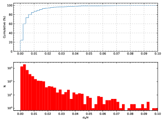
Fig. 1 : The histogram of relative parallax errors, $\sigma_{\pi}/\pi$, of 3344 main-sequence stars (lower panel) and their cumulative distribution (upper panel).

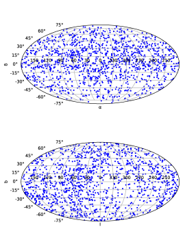
Fig. 2 : The positions of 1377 F-G type main-sequence stars on the equatorial (upper panel) and Galactic (lower panel) coordinates.

To obtain the UBV photometric data of 2959 main-sequence stars, we scanned the catalogues of Oja (1984); Mermilliod (1987, 1997); Koen et al. (2010), by considering the equatorial coordinates. Thus, we reached the UBV photometric data of 1377 stars. Distributions of stars according to equatorial and Galactic coordinates are shown in Fig. 2. The star sample was divided into three different Galactic latitude intervals, $|b|\leq 30^{o}$, $30^{o}<|b|\leq 60^{o}$ and $60^{o}<|b|\leq 90^{o}$. We found that the number of stars in these intervals are 693, 476, and 208, respectively. According to these results, about half of the programme stars are located at low Galactic latitudes. In this study, we used the dust map of Schlafly & Finkbeiner (2011) in order to remove the absorption and reddening effects of the interstellar medium. Since the absorption in a star’s direction obtained from the dust map is given for the Galactic border, this absorption value should be reduced to the distance between the Sun and the relevant star. We adopted the total absorption $A_{\infty}(b)$ in V-band for a star’s direction obtained from the dust map of Schlafly & Finkbeiner (2011) and estimated absorption $A_{d}(b)$ for the distance between Sun and the star using the following equation of Bahcall & Soneira (1980):

$$A_{d}(b)=A_{\infty}(b)\Biggl{[}1-\exp\Biggl{(}\frac{-\mid d~{}\sin(b)\mid}{H}\Biggr{)}\Biggr{]}.$$ (1)

Here, $d$ and $b$ denote the distance of the star and Galactic latitude, respectively. $H$ is the scale height of the Galactic dust ($H=125$ pc; Marshall et al., 2006). We calculated the distances of the stars from Gaia DR2 trigonometric parallaxes using the equation of $d=1000/\pi$ (mas). The colour excess of the star ($E_{d}(B-V)$) in question could be calculated from Eq. (2) (Cardelli et al., 1989) and the colour excess $E_{d}(U-B)$ was found using Eq. (3) (Garcia et al., 1988):

$$E_{d}(B-V)=A_{d}(b)/3.1,$$ (2)

$$E_{d}(U-B)=0.72\times E_{d}(B-V)+0.05\times E_{d}(B-V)^{2}.$$ (3)

The de-reddened apparent magnitude ($V_{0}$) and colour indices ($(U-B)_{0}$ and $(B-V)_{0}$) are then calculated by following equations,

$$V_{0}=V-3.1\times E_{d}(B-V),$$ (4)

$$(U-B)_{0}=(U-B)-E_{d}(U-B),$$

$$(B-V)_{0}=(B-V)-E_{d}(B-V).$$

The original $E_{\infty}(B-V)$ and reduced $E_{d}(B-V)$ colour excesses of 1377 stars are shown in Fig. 3a and 3b, respectively.

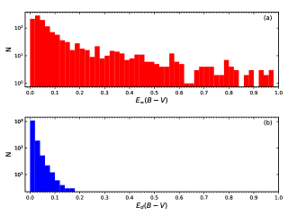
Fig. 3 : Histograms of the original $E_{\infty}(B-V)$ (a) and reduced $E_{d}(B-V)$ (b) colour excesses of 1377 F-G type main-sequence stars.

Moreover, another constraint was applied to de-reddened colour excesses $(B-V)_{0}$ of the selected programme stars. For the photometric selection of F-G type main-sequence stars, we used the $0.3<(B-V)_{0}<0.8$ mag colour index interval given by Eker et al. (2018), decreasing the number of stars in the sample to 876. A final limitation to the sample has also been made according to the photometric variability of the stars. By removing the stars with registered information such as variable stars, chromospherically active stars, pulsating stars etc. in the Simbad database, we reduced the sample to 504 stars. The spectroscopic, photometric, and astrometric data of the 504 calibration stars are listed in Table 2.

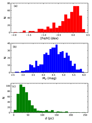
Fig. 4 : The distribution of spectroscopic metal abundances (a), $M_{V}$ absolute magnitudes estimated from the Gaia DR2 trigonometric parallaxes (b), and distances to the Sun of the calibration stars (c).

Table 2 : The basic parameters of 504 calibration stars; ID, equatorial coordinates in J2000 ($\alpha$, $\delta$), photometric data ($V$, $U-B$, $B-V$), reduced colour excess ($E_{d}(B-V)$), atmospheric model parameters ($T_{eff}$, $\log g$ and [Fe/H]) and their references (Bibcode), and trigonometric parallaxes ($\pi$) taken from Gaia DR2. Parallax errors of the stars are given in brackets.

ID	Star	$\alpha$	$\delta$	$V$	$U-B$	$B-V$	$E_{d}(B-V)$	$T_{eff}$	$\log g$	[Fe/H]	Bibcode	$\pi$	$\pi_{err}$
		(hh:mm:ss.ss)	(dd:mm:ss.s)	(mag)	(mag)	(mag)	(mag)	(K)	(cm s-2)	(dex)		(mas)	(mas)
1	HD 224930	00 02 10.34	+27 04 54.48	5.744	0.051	0.673	0.002	5454	4.54	-0.73	2017AJ….153…21L	79.0696	0.5621
2	HD 225297	00 05 02.63	$-$36 00 54.43	7.730	0.010	0.540	0.004	6181	4.55	-0.09	2017A&A…606A..94D	19.6250	0.0570
3	HD 142	00 06 19.18	$-$49 04 30.68	5.700	0.022	0.516	0.002	6403	4.62	0.09	2017A&A…606A..94D	38.1605	0.0648
4	HD 166	00 06 36.78	+29 01 17.41	6.100	0.325	0.752	0.002	5481	4.52	0.08	2017AJ….153…21L	72.5764	0.0498
5	HD 400	00 08 40.94	+36 37 37.65	6.174	-0.066	0.492	0.005	6203	4.07	-0.23	2014A&A…562A..71B	30.6749	0.0522
…	…	…	…	…	…	…	…	…	…	…	…	…	…
…	…	…	…	…	…	…	…	…	…	…	…	…	…
…	…	…	…	…	…	…	…	…	…	…	…	…	…
499	HD 224022	23 54 38.62	$-$40 18 00.22	6.019	0.107	0.574	0.002	6236	4.46	0.21	2014A&A…562A..71B	35.2618	0.0780
501	HD 224383	23 57 33.52	$-$09 38 51.07	7.863	0.146	0.641	0.011	5833	4.39	0.02	2014A&A…562A..71B	19.4670	0.0642
502	HD 224465	23 58 06.81	+50 26 51.64	6.640	0.190	0.665	0.006	5722	4.30	0.06	2015A&A…580A..24D	41.6957	0.0541
503	HD 224619	23 59 28.43	$-$20 02 04.97	7.468	0.284	0.744	0.004	5436	4.39	-0.20	2017A&A…606A..94D	38.1312	0.0519
504	HD 224635	23 59 29.29	+33 43 25.88	5.810	0.020	0.520	0.005	6227	4.36	0.03	2017AJ….153…21L	33.7083	0.0406

The histograms of the spectroscopic metallicities ([Fe/H]), the absolute magnitudes ($M_{V}$) estimated from Gaia DR2 trigonometric parallaxes (Gaia Collaboration et al., 2018) using $M_{V}=V-5\log(1000/\pi)+A_{V}$ equation, and distances ($d$) to the Sun calculated from $d=1000/\pi$ equation for 504 F-G type main-sequence stars are shown in Fig. 4. The metallicity interval of the stars is $-2<{\rm[Fe/H]}<0.5$ dex, and 81% of the sample is concentrated in the $-0.6<{\rm[Fe/H]}<0.5$ dex metallicity interval. These results show that the vast majority of stars in the sample belong to the thin-disc population of the Galaxy (Cox, 2000). Considering the histogram of the absolute magnitude of the sample, the stars are found in the $2.5<M_{V}<6$ absolute magnitude interval and frequencies of the stars are close to each other in the $4<M_{V}\leq 5.3$ mag interval. It should be noted that the maximum distance of the sample stars to the Sun is about $d=250$ pc, while 91% of the sample is within $d=100$ pc.

The calibration stars were divided six metal abundance intervals, and positions of the sample stars in the $(U-B)_{0}\times(B-V)_{0}$ two-colour and $M_{V}\times(B-V)_{0}$ colour-absolute magnitude diagrams were studied in accordance with metal abundances (Fig. 5). When the stars in the sample were plotted on the $(U-B)_{0}\times(B-V)_{0}$ two-colour diagram according to metallicity, it was determined that the UV excesses of the metal-poor stars are larger than the metal-rich ones (Fig. 5a). Also, in the $M_{V}\times(B-V)_{0}$ colour-absolute magnitude diagram (Fig. 5b), we found that the metal-poor stars have larger absolute magnitudes than metal-rich stars. As a result, it has been shown that metal abundance and absolute magnitude calibrations can be made by using photometric data of 504 calibration stars, which are selected according to spectroscopic, photometric and astrometric data.

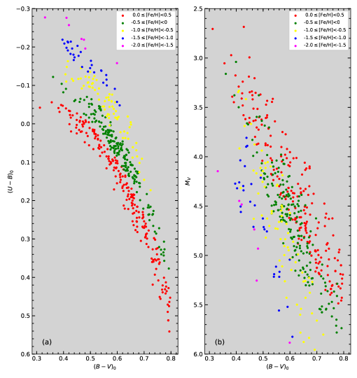
Fig. 5 : The positions of the 504 main-sequence stars on the $(U-B)_{0}\times(B-V)_{0}$ two-colour (a) and $M_{V}\times(B-V)_{0}$ colour-absolute magnitude (b) diagrams according to their metal abundances.

Table 3 : Coefficients and their errors for the Eq. (5). Errors are given in brackets.

Coefficient	$a_{1}$	$b_{1}$	$c_{1}$	$d_{1}$	$e_{1}$	$f_{1}$
Value	-4.7503	-8.395	2.141	5.236	3.775	0.1597
	(0.7624)	(1.476)	(1.062)	(1.118)	(1.575)	(0.0418)

3 Method

3.1 Metallicity calibration

We used precise spectroscopic, photometric, and astrometric data of 504 F-G type main-sequence stars to construct a photometric metallicity calibration. The following Eq. (5) between $(U-B)_{0}$ and $(B-V)_{0}$ colour indices and spectroscopic metal abundances of calibration stars were adopted and the parameters of variables were calculated by the multiple regression method:

$${\rm[Fe/H]}=a_{1}(U-B)_{0}^{2}+b_{1}(B-V)_{0}^{2}+c_{1}(U-B)_{0}(B-V)_{0}$$ (5)

$$+d_{1}(U-B)_{0}+e_{1}(B-V)_{0}+f_{1}$$

The calculated parameters and their errors are listed in Table 3. The correlation coefficient and standard deviation of the metallicity calibration (Eq. 5) are $R^{2}=0.932$ and $\sigma=0.11$ dex, respectively. Comparison of estimated photometric metal abundances (${\rm[Fe/H]}_{est}$) with original spectroscopic metal abundances (${\rm[Fe/H]}_{org}$) and differences between these values ($\Delta{\rm[Fe/H]}={\rm[Fe/H]}_{org}-{\rm[Fe/H]}_{est}$) are shown in Fig. 6. The mean value and standard deviation of the differences between estimated and original metal abundances are $\langle{\rm[Fe/H]}\rangle=0.00$ and $\sigma_{\rm[Fe/H]}=0.11$ dex, respectively. The upper panel of Fig. 6 shows that the distribution becomes denser around the one-to-one line and the scattering of the metal abundance differences is relatively small. The lower panel of Fig. 6 represents that metal abundance differences between estimated from the above calibration equation (Eq. 5) and spectroscopic data are in the range of $\pm 0.26$ dex and most of the difference values are within $\pm 1\sigma$.

Table 4 : Coefficients and their errors for the Eq. (6). Errors are given in brackets.

Coefficient	$a_{2}$	$b_{2}$	$c_{2}$	$d_{2}$	$e_{2}$	$f_{2}$
Value	4.382	17.242	-10.620	0.547	-7.885	3.4576
	(1.477)	(2.861)	(3.996)	(0.167)	(3.052)	(0.8104)

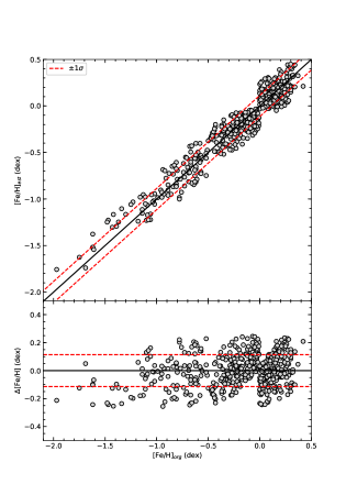
Fig. 6 : Comparison of the estimated (${\rm[Fe/H]}_{est}$, photometric) and the original (${\rm[Fe/H]}_{org}$, spectroscopic) metallicities (upper panel) and distribution of the metallicity residuals $\Delta$[Fe/H] with respect to the original metallicities (lower panel) for 504 calibration stars. The black solid line represents one-to-one line and dashed red lines denote $\pm 1\sigma$ prediction levels.

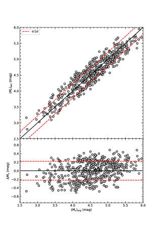
Fig. 7 : Comparison of the estimated ($(M_{V})_{est}$ photometric) and the original ($(M_{V})_{org}$, Gaia trigonometric parallaxes) absolute magnitudes (upper panel) and distribution of the absolute magnitude residuals $\Delta M_{V}$ with respect to the original absolute magnitudes (lower panel) for 504 calibration stars. The black solid line represents one-to-one line and dashed red lines denote $\pm 1\sigma$ prediction levels.

3.2 Absolute magnitude calibration

To construct an absolute magnitude ($M_{V}$) calibration in the UBV photometric system, we used 504 F-G type main-sequence stars in our data sample. The absolute magnitudes of these calibration stars were obtained with the equation, $M_{V}=V-5\log(1000/\pi)+A_{V}$, and the distances of stars in this equation were calculated from the Gaia DR2 trigonometric parallaxes (Gaia Collaboration et al., 2018). The following Eq. (6) between $(U-B)_{0}$ and $(B-V)_{0}$ colour indices and absolute magnitude of calibration stars was adopted and the parameters of variables were calculated by the multiple regression method:

$$M_{V}=a_{2}(U-B)_{0}^{2}+b_{2}(B-V)_{0}^{2}+c_{2}(U-B)_{0}(B-V)_{0}$$ (6)

$$+d_{2}(U-B)_{0}+e_{2}(B-V)_{0}+f_{2}$$

The calculated parameters and their errors are listed in Table 3. The correlation coefficient and standard deviation of the absolute magnitude calibration (Eq. 6) are $R^{2}=0.869$ and $\sigma=0.22$ mag, respectively. Comparison of estimated absolute magnitude ($(M_{V})_{est}$) with original (from Gaia trigonometric parallaxes) absolute magnitudes ($(M_{V})_{org}$) and differences between these values ($\Delta M_{V}=(M_{V})_{org}-(M_{V})_{est}$) are shown in Fig. 7. The mean value and standard deviation of the differences between estimated and original absolute magnitudes are $\langle M_{V}\rangle=0.00$ and $\sigma_{\langle M_{V}\rangle}=0.22$ mag, respectively. The upper panel of Fig. 7 shows that the distribution becomes denser around the one-to-one line and the scattering of the absolute magnitude differences is relatively small. The lower panel of Fig. 7 represents that absolute magnitude differences calculated from two different methods are in the range of $\pm 0.51$ mag and most of the differences are within $\pm 1\sigma$.

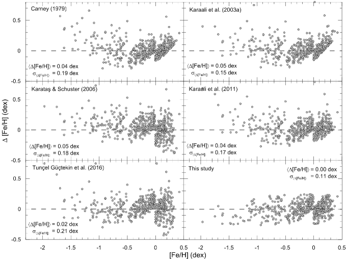
Fig. 8 : Distributions of the metallicity residuals of various calibration equations estimated for 504 F-G spectral type main-sequence stars with respect to the metallicities in this study. The reference for the calibration in question is indicated in each panel, together with mean value and standard deviation of residuals.

4 Summary and Discussion

Using precise spectroscopic ($T_{eff}$, $\log g$ and [Fe/H]), photometric ($V$, $U-B$, $B-V$) and astrometric ($\pi$) data of F and G spectral type main-sequence stars, new calibrations for the UBV photometry were obtained to estimate the metallicities and absolute magnitudes photometrically. Tough limitations on spectroscopic, photometric, and astrometric data were made to select the calibration stars, reducing the number of stars in the sample from 5756 to 504. Multiple regression method was used to construct new metal abundance and absolute magnitude calibrations, which would be a connection between the photometric data of the stars, metal abundances from spectroscopic studies and trigonometric parallaxes determined by astrometric methods. When calculating metal abundances and absolute magnitudes of F-G type main sequence stars in low Galactic latitudes using photometric calibrations, it should be noted that they are exposed to extreme interstellar medium and the colour excess should be sensitively determined.

4.1 Comparison of new metallicity calibration with those in the literature

In the literature, the relationships with polynomials of different degrees between the UV residuals of the stars and spectroscopic metallicities were used. For about 60 years, the application of similar methods to main-sequence stars, increasing photometric, spectroscopic and astrometric sensitivities with the developing technology have affected sensitivities of the calibrations. In the literature, five studies attract our attention when the UV residuals-sensitive metallicity calibrations for the UBV photometry are investigated: Carney (1979), Karaali et al. (2003a), Karataş & Schuster (2006), Karaali et al. (2011), and Tunçel Güçtekin et al. (2016). Analytical expressions of the metallicity calibrations in these studies reveal that the colour index of the calibrations depends on the UV residuals ($\delta_{0.6}$) normalized to $(B-V)_{0}=0.6$ mag. The primary difference between the metallicity calibrations is that the photometric UV residuals of the stars are expressed in different degrees of polynomials. We applied the five aforementioned metallicity calibrations to 504 stars in our sample for a further comparison of our results with the ones in these studies. The distributions of differences ($\Delta{\rm[Fe/H]}$) between photometric metallicities estimated from the calibration in each study and the original spectroscopic metallicities are shown in Fig. 8 according to the spectroscopic ones (${\rm[Fe/H]}_{org}$).

Note that similar distributions are obtained by taking into account the validity limits of the metallicity calibrations. While the means of metallicity differences ($\Delta{\rm[Fe/H]}$) in four studies (Carney, 1979; Karaali et al., 2003a, 2011; Karataş & Schuster, 2006) are between 0.04 and 0.05 dex, these values are lower than 0.02 dex for two studies (Tunçel Güçtekin et al., 2016, and this study). As for the dispersion of metallicity distributions, the smallest standard deviation value is obtained in this study, $\sigma=0.11$ dex. The standard deviations of metallicity differences range from 0.15 to 0.21 dex in previous studies. Thus, we conclude that the metallicity calibration derived in this study is more reliable than those in the literature, considering the mean metallicity differences and standard deviations.

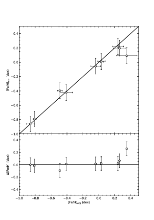
Fig. 9 : Comparison of the estimated (${\rm[Fe/H]}_{est}$) and the original (${\rm[Fe/H]}_{org}$) metallicities of 10 Gaia benchmark stars which are taken from Jofré et al. (2015).

Another study to compare our photometric metallicity calibrations was also described by Jofré et al. (2015). They obtained iron and alpha element abundances of 34 Gaia FGK benchmark stars using eight different spectral analysis methods. Since the spectral resolution and $S/N$ of the 34 stars used in their study were quite good, the element abundances of the stars were determined with high sensitivity. In order to see the sensitivity of the new metallicity calibration produced in our study, these Gaia benchmark stars are taken into consideration. In this comparison, we used 10 main-sequence stars within the range of $-2<{\rm[Fe/H]}<0.5$ dex metallicity interval and UBV photometric data available. Photometric metal abundances were determined for these stars using our methods described in Sections 2 and 3. Comparison of estimated photometric metal abundance with spectroscopic ones are shown in Fig. 9. As shown in this figure, metal abundances of 10 stars obtained from two different methods are quite compatible with each other within the errors, except for $\mu$ Ara which has the richest metallicity in the sample. Considering 47 spectroscopic studies of $\mu$ Ara in the literature, it is seen that the metal abundance is in the range of $0.16<[{\rm Fe/H}]<0.41$ dex (Francois, 1986; Hearnshaw, 1975) and the median metallicity of the star is [Fe/H]=0.28 dex. The median metallicity of the star and the photometric metal abundance calculated in this study ([Fe/H]=0.10 dex) is more compatible within the errors. This result shows that our photometric metallicity calibration can be used in the calculation of metal abundances of F-G main-sequence stars with an accuracy of $\pm 0.11$ dex in the range $-2<{\rm[Fe/H]}<0.5$ dex, where it is valid.

Our new metallicity calibration has two superior aspects compared to similar studies in the literature. At first, it uses a large number of main-sequence stars having precise spectroscopic, photometric and astrometric data, and the other one is that it is possible to determine the photometric metallicity of F-G spectral type main-sequence stars without depending on a standardized UV residual.

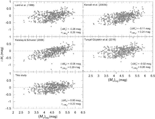
Fig. 10 : Distributions of the absolute magnitude residuals of various calibration equations estimated for 504 F-G spectral type main-sequence stars with respect to the absolute magnitudes in this study. The reference for the calibration in question is indicated in each panel, together with mean value and standard deviation of residuals.

4.2 Comparison of new absolute magnitude calibration with those in the literature

In the literature, there are four studies regarding to the UV residuals-sensitive absolute magnitude calibrations: Laird et al. (1988), Karaali et al. (2003b), Karataş & Schuster (2006) and Tunçel Güçtekin et al. (2016). Common aspects of these studies, in which different photometric and trigonometric parallax data obtained in different times were used, are that their calibrations are expressed by third degree polynomial functions, they depend on UV residuals and that the main-sequence members of the Hyades open cluster are used as reference in the calculations.

The absolute magnitude calibration in this study was compared with the calibrations of the four research groups in the literature. For comparisons, 504 F-G spectral type main-sequence stars in our study were placed in the calibration relation of each study and the absolute magnitudes of the stars were calculated. The differences $\Delta M_{V}$ between the absolute magnitudes calculated from Gaia parallaxes and those obtained from the calibrations are shown in Fig. 10. The absolute magnitudes of the stars calculated from the calibrations are in the $2.5<M_{V}<6$ mag interval and the differences are found to be in the $-1.5<\Delta M_{V}<+1$ mag interval. In general, the calculated absolute magnitude differences of the stars in $M_{V}<3$ and $M_{V}>5.5$ mag contain systematic errors in the previous calibrations. The absolute magnitude differences calculated from the calibration of Karataş & Schuster (2006) are compatible with the Gaia DR2 only for a very limited range of absolute magnitudes, containing larger systematic errors. The distribution of absolute magnitude differences reveal that the most incompatible calibration study was performed by Laird et al. (1988), while the calibrations of Karaali et al. (2003b) and Karataş & Schuster (2006) seem to follow it. The results of this study and Tunçel Güçtekin et al. (2016) presents the most compatible absolute magnitudes with those of calculated from Gaia DR2, compared to the absolute magnitudes estimated from the previous calibrations. The mean values and standard deviations of the absolute magnitude differences are -0.28 and 0.26 mag, -0.11 and 0.24 mag, -0.08 and 0.29 mag, -0.02 and 0.26 mag, and 0.02 and 0.22 mag, for Laird et al. (1988), Karaali et al. (2003b), Karataş & Schuster (2006), Tunçel Güçtekin et al. (2016) and this study, respectively. In terms of the mean values and standard deviations of absolute magnitude differences, we conclude that the calibration suggested in this study is very reliable.

The application of new calibrations to the main-sequence stars can be used to predict metal abundances and distances, and in the investigation of the formation and evolution of our Galaxy (Karaali et al., 2003a, b; Bilir et al., 2005; Ak et al., 2007; Juric et al., 2008; Ivezic et al., 2008; Siegel et al., 2009; Karaali et al., 2011; Tunçel Güçtekin et al., 2016, 2017, 2019). In addition, it could be preferable to determine the mean metallicities and distances of clusters by determining metallicities of member stars of open and globular clusters (see Karaali et al., 2003c, 2014; Bilir et al., 2006, 2010, 2013, 2016; Yontan et al., 2015, 2019; Bostancı et al., 2015, 2018; Ak et al., 2016).

5 Acknowledgments

We thank the anonymous referees for their insightful and constructive suggestions, which significantly improved the paper. This research has made use of the SIMBAD, NASA’s Astrophysics Data System Bibliographic Services and the NASA/IPAC Infrared Science Archive, which is operated by the Jet Propulsion Laboratory, California Institute of Technology, under contract with the National Aeronautics and Space Administration. This work has made use of data from the European Space Agency (ESA) mission Gaia (https://www.cosmos.esa.int/gaia), processed by the Gaia Data Processing and Analysis Consortium (DPAC). Funding for the DPAC has been provided by national institutions, in particular the institutions participating in the Gaia Multilateral Agreement.

References

- Ak et al. (2007) Ak, S., Bilir, S., Karaali, S., Buser, R., Cabrera-Lavers, A., 2007, NewA, 12, 605
- Ak et al. (2016) Ak, T., Bostancı, Z. F., Yontan, T., Bilir, S., Güver, T., Ak, S., Ürgüp, H., Paunzen, E., 2016, Ap&SS, 361, 126
- Allende Prieto et al. (2008) Allende Prieto, C., Majewski, S. R., Schiavon, R., et al., 2008, AN, 329, 1018
- Bahcall & Soneira (1980) Bahcall, J. N., Soneira, R. M., 1980, ApJS, 44, 73
- Battistini & Bensby (2016) Battistini, C., Bensby, T., 2016, A&A, 586, 49
- Beers et al. (2017) Beers, T. C., Placco, V. M., Carollo, D., et al., 2017, ApJ, 835, 81
- Bensby et al. (2014) Bensby, T., Feltzing, S., Oey, M. S., 2014, A&A, 562, A71
- Bilir et al. (2005) Bilir, S., Karaali, S., Tunçel, S., 2005, AN, 326, 321
- Bilir et al. (2006) Bilir, S., Karaali, S., Güver, T., Karataş, Y., Ak, S., 2006, AN, 327, 72
- Bilir et al. (2008) Bilir, S., Karaali, S., Ak, S., Yaz, E., Cabrera-Lavers, A., Coşkunoğlu, K. B., 2008, MNRAS, 390, 1569
- Bilir et al. (2009) Bilir, S., Karaali, S., Ak, S., Coşkunoğlu, K. B., Yaz, E., Cabrera-Lavers, A., 2009, MNRAS, 396, 1589
- Bilir et al. (2010) Bilir, S., Güver, T., Khamitov, I., Ak, T., Ak, S., Coşkunoğlu, K. B., Paunzen, E., Yaz, E., 2010, Ap&SS, 326, 139
- Bilir et al. (2013) Bilir, S., Ak, T., Ak, S., Yontan, T., Bostancı, Z. F., 2013, NewA, 23, 88
- Bilir et al. (2016) Bilir, S., Bostancı, Z. F., Yontan, T., et al., 2016, AdSpR, 58, 1900
- Boesgaard et al. (2011) Boesgaard, A. M., Rich, J. A., Levesque, E. M., et al., 2011, ApJ, 743, 140
- Bostancı et al. (2015) Bostancı, Z. F., Ak, T., Yontan, T., et al., 2015, MNRAS, 453, 1095
- Bostancı et al. (2018) Bostancı, Z. F., Yontan, T., Bilir, S., et al., 2018, Ap&SS, 363, 143
- Brewer et al. (2016) Brewer, J. M., Fischer, D. A., Valenti, J. A., Piskunov, N., 2016, ApJS, 225, 32
- Buser & Fenkart (1990) Buser, R., Fenkart, R. P., 1990, A&A, 239, 243
- Cameron (1985) Cameron, L. M., 1985, A&A, 152, 250
- Cardelli et al. (1989) Cardelli, J. A., Clayton, G. C., Mathis, J. S., 1989, ApJ, 345, 245
- Carney (1979) Carney, B. W., 1979, AJ, 84, 515
- Chonis & Gaskell (2008) Chonis, T. S., Gaskell, C. M., 2008, AJ, 135, 264
- Cox (2000) Cox, A. N., 2000. Allen’s astrophysical quantities, 4th ed. Publisher: New York: AIP Press; Springer, 2000. Edited by Arthur N. Cox. ISBN: 0387987460
- da Silva et al. (2015) da Silva, R., Milone, A. De C., Rocha-Pinto, H. J., 2015, A&A, 580, 24
- de Silva et al. (2015) de Silva, G. M., Freeman, K. C., Bland-Hawthorn, J., et al., 2015, MNRAS, 449, 2604
- Delgado Mena et al. (2017) Delgado Mena, E., Tsantaki, M., Adibekyan, V. Zh., Sousa, S. G., Santos, N. C., Gonzalez Hernandez, J. I., Israelian, G., 2017, A&A, 606A, 94
- Eker et al. (2018) Eker, Z., Bakış, V., Bilir, S., et al., 2018, MNRAS, 479, 5491
- ESA (1997) ESA, 1997, The Hipparcos and Tycho catalogues. Publisher: Noordwijk, Netherlands: ESA Publications Division 1997, Series: ESA SP Series vol no: 1200, ISBN: 9290923997
- Francois (1986) Francois, P., 1986, A&A, 165, 183
- Gaia Collaboration et al. (2018) Gaia Collaboration, Brown, A. G. A., Vallenari, A., et al., 2018, A&A, 616, 22
- Garcia et al. (1988) Garcia, B., Claria, J. J., Levato, H., 1988, Ap&SS, 143, 317
- Gilmore et al. (2012) Gilmore, G., Randich, S., Asplund, M., et al., 2012, The Messenger, 147, 25
- Hearnshaw (1975) Hearnshaw, J. B., A&A, 38, 271
- Helmi et al. (2018) Helmi, A., Babusiaux, C., Koppelman, H. H., et al., 2018, Nature, 563, 85
- Ishigaki et al. (2012) Ishigaki, M. N., Chiba, M., Aoki, W., 2012, ApJ, 753, 64
- Ivezic et al. (2008) Ivezic, Z., Sesar, B., Juric, M., et al. 2008, 684, 2871
- Jofré et al. (2015) Jofré, P., Heiter, U., Soubiran, C., et al., 2015, A&A, 582A, 81
- Juric et al. (2008) Juric, M., Ivezic, Z., Brooks, A., et al., 2008, ApJ, 673, 864
- Karaali et al. (2003a) Karaali, S., Bilir, S., Karataş, Y., Ak, S. G., 2003a, PASA, 20, 165
- Karaali et al. (2003b) Karaali, S., Karataş, Y., Bilir, S., Ak, S. G., Hamzaoğlu, E., 2003b, PASA, 20, 270
- Karaali et al. (2003c) Karaali, S., Ak, S. G., Bilir, S., Karataş, Y., Gilmore, G., 2003c, MNRAS, 343, 1013
- Karaali et al. (2005) Karaali, S., Bilir, S., Tunçel, S., 2005, PASA, 22, 24
- Karaali et al. (2011) Karaali, S., Bilir, S., Ak, S., Yaz, E., Coşkunoğlu, B., 2011, PASA, 28, 95
- Karaali et al. (2014) Karaali, S., Gökçe Yaz, E., Bilir, S., Tunçel, S., 2014, PASA, 31, 27
- Karataş & Schuster (2006) Karataş, Y., Schuster, W., 2006, MNRAS, 371, 1793
- Koen et al. (2010) Koen, C., Kilkenny, D., van Wyk, F., Marang, F., 2010, 403, 1949
- Kunder et al. (2012) Kunder, A., Koch, A., Rich, R. M., et al., 2012, AJ, 143, 57
- Laird et al. (1988) Laird, J. B., Carney, B. W., Latham, D. W., 1988, AJ, 95, 1843
- Luck (2017) Luck, R. E., 2017, AJ, 153, 21
- Lutz & Kelker (1973) Lutz, T. E., Kelker, D. H., 1973, PASP, 85, 573
- Maldonado & Villaver (2016) Maldonado, J., Villaver, E., 2016, A&A, 588, 98
- Marshall et al. (2006) Marshall, D. J., Robin, A. C., Reylé, C., Schultheis, M., Picaud, S., 2006, A&A, 453, 635
- Mermilliod (1987) Mermilliod, J. C., 1987, A&AS, 71, 413
- Mermilliod (1997) Mermilliod, J. C., 1997, yCat, 2168, 0
- Mishenina et al. (2013) Mishenina, T. V., Pignatari, M., Korotin, S. A., Soubiran, C., Charbonnel, C., Thielemann, F. -K., Gorbaneva, T. I., Basak, N. Y., 2013, A&A, 552A, 128
- Molenda-Zakowicz et al. (2013) Molenda-Zakowicz, J., Sousa, S. G., Frasca, A., et al., 2013, MNRAS, 434, 1422
- Nissen & Schuster (2011) Nissen, P. E., Schuster, W. J., 2011, A&A, 530A, 15
- Oja (1984) Oja, T., 1984, A&AS, 57, 357
- Robin et al. (2014) Robin, A. C., Reyle, C., Fliri, J., et al., 2014, A&A, 259A, 13
- Roman (1955) Roman, N. G., 1955, ApJS, 2, 195
- Sales et al. (2009) Sales, L. V., Helmi, A., Abadi, M. G., et al., 2009, MNRAS, 400, 61
- Sandage & Eggen (1959) Sandage, A., Eggen, O. J., 1959, MNRAS, 119, 278
- Sandage (1969) Sandage, A., 1969, ApJ, 158, 1115
- Schlafly & Finkbeiner (2011) Schlafly, E. F., Finkbeiner, D. P., 2011, ApJ, 737, 103
- Schwarzschild et al. (1955) Schwarzschild, M., Searle, L., Howard, R., 1955, ApJ, 122, 353
- Siegel et al. (2009) Siegel, M. H., Karataş, Y., Reid, I. N., 2009, MNRAS, 395, 1569
- Sitnova et al. (2015) Sitnova, T., Zhao, G., Mashonkina, L., et al., 2015, ApJ, 808, 148
- Smith (1987) Smith, H., Jr., 1987, A&A, 188, 233
- Steinmetz et al. (2006) Steinmetz, M., Zwitter, T., Siebert, A., et al., 2006, ApJ, 132, 1645
- Strömgren (1966) Strömgren, B., 1966, ARA&A, 4, 433
- Trefzger et al. (1995) Trefzger, Ch. F., Pel, J. W., Gabi, S., 1995, A&A, 304, 381
- Tunçel Güçtekin et al. (2016) Tunçel Güçtekin, S., Bilir, S., Karaali, S., Ak, S., Ak, T., Bostancı, Z. F., 2016, Ap&SS, 361, 18
- Tunçel Güçtekin et al. (2017) Tunçel Güçtekin, S., Bilir, S., Karaali, S., Plevne, O., Ak, S., Ak, T., Bostancı, Z. F., 2017, Ap&SS, 362, 17
- Tunçel Güçtekin et al. (2019) Tunçel Güçtekin S., Bilir, S., Karaali, S., Plevne, O., Ak, S., 2019, AdSpR, 63, 1360
- van Leeuwen (2007) van Leeuwen, F., 2007, A&A, 474, 653
- Wallerstein (1962) Wallerstein, G., 1962, ApJS, 6, 407
- Walraven & Walraven (1960) Walraven, Th., Walraven, J. H., 1960, Bulletin of the Astronomical Institutes of the Netherlands, 15, 67
- Yanny et al. (2009) Yanny, B., Rockosi, C., Newberg, H. J., et al., 2009, AJ, 137, 4377
- Yontan et al. (2015) Yontan, T., Bilir, S., Bostancı, Z. F., et al., 2015, Ap&SS, 355, 267
- Yontan et al. (2019) Yontan, T., Bilir, S., Bostancı, Z. F., et al., 2019, Ap&SS, 364, 152
- York et al. (2000) York, D. G., Adelman, J., Anderson, J. E., et al., 2000, AJ, 120, 1579
- Zhao et al. (2012) Zhao, G., Zhao, Y., Chu, Y., et al., 2012, RAA, 12, 723