A Machine Learning Framework for Sleeping Cell Detection in a Smart-city IoT Telecommunications Infrastructure

Abstract

The smooth operation of largely deployed Internet of Things (IoT) applications will depend on, among other things, effective infrastructure failure detection. Access failures in wireless network Base Stations produce a phenomenon called “sleeping cells”, which can render a cell catatonic without triggering any alarms or provoking immediate effects on cell performance, making them difficult to discover. To detect this kind of failure, we propose a Machine Learning (ML) framework based on the use of Key Performance Indicators statistics from the BS under study, as well as those of the neighboring BSs with propensity to have their performance affected by the failure. A simple way to define neighbors is to use adjacency in Voronoi diagrams. In this paper, we propose a much more realistic approach based on the nature of radio-propagation and the way devices choose the BS to which they send access requests. We gather data from large-scale simulators that use real location data for BSs and IoT devices and pose the detection problem as a supervised binary classification problem. We measure the effects on the detection performance by the size of time aggregations of the data, the level of traffic and the parameters of the neighborhood definition. The Extra Trees and Naive Bayes classifiers achieve Receiver Operating Characteristic (ROC) Area Under the Curve (AUC) scores of $0.996$ and $0.993$, respectively, with False Positive Rates under $5\%$. The proposed framework holds potential for other pattern recognition tasks in smart-city wireless infrastructures, that would enable the monitoring, prediction and improvement of the Quality of Service (QoS) experienced by IoT applications.

=-15pt

I Introduction

The deployment of the IoT in urban areas is enabling the creation of so-called “smart cities” where city life will be improved by using large amounts of information coming from hundreds of thousands of geographically distributed communicating devices. This information will lead to the automation of some systems and the creation of new applications that will enhance city living. Smart parking, smart pedestrian crossings, intelligent transportation systems, and intelligent power distribution are just a few of the new types of innovations that can be put in place with the effective exchange of information between city IoT devices. IoT-enabled data and services in smart cities rely on either (a) users interacting with smart devices connected to the Internet or (b) users using network services that depend on IoT devices serving as sensors or actuators [1]. In both cases, communications are essential for the IoT applications to work.

Even though several telecommunication technologies have been proposed for the deployment of different IoT applications in cities [2, 3], the ubiquity of cellular communications is making operators and standardization entities such as the $3^{rd}$ Generation Partnership Project (3GPP) push for a common cellular infrastructure for smart cities based on $4^{th}$ Generation of broadband cellular network technology (4G) enhancements and $5^{th}$ Generation (5G).

Even with the use of a common communication infrastructure, there are several drawbacks of smart-city large-scale implementation. First, it heavily depends on reliable telecommunications, as even banal failures may lead to the massive malfunctioning of key automated systems. Second, the type of telecommunication traffic produced in smart cities will mostly be produced by IoT machines inside those automated systems. The problem is that the statistical behaviour of this traffic is quite different from that produced by humans [4], and the lack of direct human interaction will make it even more difficult to detect telecommunication failures. Finally, the distributed nature of the applications and the large number of devices and connections will also hinder failure detection.

One of the most difficult types of failure to detect in cellular networks is the so-called “sleeping cell” failure. It consists of failures that will not set-off alarms even if the cell is malfunctioning. In human cellular communications, a sleeping cell will cause users to react to the lack of service, change location and eventually notify the operator. This failure can be prolonged, in some cases days, before being detected by the operator, and corrective measures are taken[5]. The influence of sleeping cell failures is greatly amplified in smart cities, where many automated systems may depend on the normal function of a particular cell. Thus, the city does not have the luxury of waiting several days for the malfunctioning cell to be detected. The delay constraints of essential smart-city applications might be difficult to satisfy even with fully-operational BSs due to the massive number of devices that are expected to request access [6].

The objective of this paper is to present a ML framework to detect sleeping cells in a smart-city IoT context. The framework is based on the following:

• the introduction of a novel concept of neighborhood between BSs, and

• the use of aggregated KPIs over time intervals for different types of IoT applications.

The data used to feed our framework were extracted from a large-scale IoT infrastructure simulator that takes as its input a real city database of geographical locations of potential IoT devices and the current locations and features of the BSs of several service providers.

In the remainder of this paper, we present the state of the art in Section II. In Section III, we present the modeling of the system, emphasizing the relationship between the infrastructure technology and the locations of the IoT devices. The ML framework is detailed in Section IV, starting with novel definitions of the cell neighborhood and proximity that are at the core of the framework, followed by the simulation and ML methodologies, and ending with some remarks on the implementation. Numerical results are shown and commented on Section V, and conclusions are presented in Section VI.

II State of the art

Failure detection of network elements is one of the main concerns of mobile network operators. Several papers in the literature address this problem using real network operator data at the BS level [7, 8, 9, 10, 11]. This approach produces very accurate results for the specific networks, but the solutions are not easily generalized due to the difficulty in retrieving real cellular network data. As a consequence, most authors use simulated data, such as in [12, 13, 14, 15, 16, 7, 10, 17, 18, 19], though emulations based on real data can also be found [20]. In this work, we employ simulated network data generated with a large-scale network simulator [21] (an extension of [4]), which employs real data on the positions of network elements and the parameters of the communicating nodes.

There has been much work dedicated to solving problems in wireless networks using ML; for an extensive survey, see [22]. A common approach in failure detection is to learn standard traffic patterns and quickly detect deviations from normal behavior (i.e., unsupervised learning). In particular, existing research focuses on i) anomaly detection [23, 24, 7], ii) KPIs [25], iii) clustering [11, 16, 14], and iv) dimensionality-reduction techniques [14, 26]. Other authors exploit known properties of cellular networks to perform supervised learning to detect faulty elements in a network [24, 11, 27, 18, 13, 19].

A complementary approach to ML proposed by [28] is to acquire data from troubleshooting (human) experts in mobile networks and to use their experience and knowledge to improve fault detection. In addition to the proposed techniques, fuzzy models can be used for failure detection, as presented in [20, 17].

Finally, some authors propose detecting failures in a network element by looking at anomalies in the traffic and KPIs from neighboring cells [10, 13, 19]. This is particularly powerful when the traffic generated in a defected cell does not present remarkable anomalies in its KPIs, such as in the case of Random-Access Channel (RACH)-sleeping cells, where new users cannot connect but existing users in the cell can continue to transmit regularly during a failure.

In this paper, we propose using well-known supervised learning techniques for BS failure detection in a smart-city cellular infrastructure. In particular, for each cell, KPIs from neighboring cells are analyzed to highlight anomalies and detect defective BSs. Different from the reviewed literature, i) we consider advanced propagation models based not only on distance but also on other parameters, such as Received Signal Strength (RSS), the bandwidth, frequency, and antenna orientation, and ii) we define different neighbor categories to improve failure detection.

III System modelling

Let us first mention that we provide in Table I a summary of the mathematical notation used in our modelling of the system as well as in the description of the proposed framework.

III-A Communication infrastructure

The cellular network model is composed of a set $\mathcal{B}$ of base stations enumerated as $\{b_{1},\dots,b_{M}\}$, a set of IoT devices in geographical locations $\{g_{1},\dots,g_{L}\}\subset\mathcal{G}$ , a backbone $\mathcal{N}$, and a Data Management Center (DMC). Only the uplink performance is considered; the core and metropolitan part of the network are modeled as a black box.

TABLE I: Summary of mathematical notation.

Symbol	Description
$\mathcal{B}$	Set of $M$ BSs $\{b_{1},...,b_{M}\}$.
$\mathcal{G}$	Set of potential geographical locations for an IoT device.
$r_{g}(i)$	RSS from a $b_{i}\in\mathcal{B}$ as measured from location $g\in\mathcal{G}$
$\mathbf{s}_{g}$	Ordered list of size $\xi$ of the $b_{g,i}\in\mathcal{B}$ with highest $r_{g}(g,i)$ values in decreasing order $\{b_{g,1},...,b_{g,\xi}\}$. Subscript $i$ indicates priority.
$f(i)$	Failure indicator for $b_{i}\in\mathcal{B}$.
$Pr(X=x)$	Probability of event $x$.
$\mathcal{C}^{n}_{i}$	Set of $b_{j}\in\mathcal{B}$ belonging to the Neighborhood Category $n$ of $b_{i}\in\mathcal{B}$.
$\mathcal{I}_{u-v}$	Ordered list of consecutive positions $\{u,u+1,...,v\}$, such that $\xi\geq v\geq u\geq 1$.
$c^{n}_{i,j}$	Category $n$ neighborhood indicator for $b_{i},b_{j}\in\mathcal{B}$.
$P^{u-v}(b_{i},b_{j})$	Indicator of $u-v$ Proximity for a pair of antennas $b_{i},b_{j}\in\emph{B}$.
$x_{i,t}$	Feature vector for $b_{i}\in\mathcal{B}$ in interval $t$.
$o(x_{i,t})$	Target value used for training of ML models.
$\mathcal{N}$	Backbone of the cellular network.

We assume a limited number of wireless channels (i.e., the Resource Blocks in Long-Term Evolution (LTE)) can be used to transmit data between users and BSs. This is done through dedicated control channels allocated through a random access procedure (RACH), based on preamble transmissions. The available preambles are limited and might collide, triggering retransmission and introducing additional delay in the communications between devices and BSs.

The key parameters in this study are the collision probability and the access delay, i.e., the time required for a user packet to be received by the associated BS. In particular, high-order statistics on those two parameters are used to detect sleeping cells. Further details on the methodology are provided in Section IV.

III-B Topology definition

The framework was built with real telecommunications and urban data from the city of Montreal (see details in [4]). In Fig. 1, a toy example of a smart-city cellular system is displayed: network users are represented by IoT devices, such as cars, buses, traffic lights, and security cameras. Details on the types of IoT device considered and their characteristics can be found in a previous work [29], where six different IoT applications are presented. The rectangle represents the geographical boundaries of a smart city, in which three BSs $b_{i}$, $b_{j}$, and $b_{k}$ are installed and provide network access to the IoT devices. The geographical position and other features of the BSs, such as the bandwidth, transmitted power, and orientation, were retrieved from [30].

Figure 1: A sample scheme of the proposed architecture with three BSs and a large number of IoT devices.

To characterize the links between users and BSs we i) define a threshold on the received power, ii) compute the power received from each of the BSs by each IoT device, and iii) determine the list of BSs that cover each IoT device. A threshold of $-100$ dBm is considered in this study. The received power is computed according to the Cost-Hata (Cost-231 defined in [31]) propagation model, which allows computing the path loss based on key parameters, such as the frequency, distance, and height. This propagation model is also combined with the corresponding radiation patterns for each BS. This leads to computing the Equivalent Isotropic Radiated Power (EIRP), based on the elevation, gain and inclination of the antennas, which are also available at [30]. The list of BSs covering a certain IoT device can be very large, especially in a densely populated urban scenario like Montreal, and this can lead to computational inefficiencies and large execution times. As a consequence, this list is limited to the $\xi$ BSs with the highest received power. The list is used, as described in Section IV-A, to combine the analysis of one cell’s KPIs with those of neighbor cells, and ultimately to detect the sleeping cells with high accuracy.

III-C The sleeping cell problem

A sleeping cell is usually defined as a cell that is not entirely operational and whose malfunctioning is not easily detectable by the network operator, as highlighted in [25]. This term is generally used to describe a wide variety of hardware and software failures, which degrade the QoS and Quality of Experience (QoE) and can remain hidden to the network operator for a long time (days or even weeks) [32]. In this study, we address a particular type of sleeping cells that affects the RACH in LTE networks [25]. On the one hand, this type of problem affects new users who are not able to complete the access procedure and consequently cannot access the network. On the other hand, existing users, which were already connected to the BS when the problem manifested, continue to transmit. As a consequence, standard methods based on traffic monitoring fail to detect the problem, because the network operator continues to monitor updated statistics coming from the RACH-sleeping BS. Progressively, all the ongoing connections end, and the cell ceases all activity.

IV A framework for sleeping cell detection

IV-A Neighborhood/closeness definition

When trying to detect if a particular BS has failed, our key idea is to include data from its “neighborhood”. However how does one determine which BSs can be considered as “neighbors”? Though the BS distance can be used, as done in [19], we now propose a richer definition: a neighboring BS is actually one whose performance KPIs are likely to be affected by the access failure in the BS under study. Accordingly, we base our definition on the following:

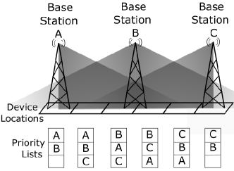
Figure 2: Priority list example.

1. Antenna priority and RSS: when sending access requests, an IoT device at location $g\in\mathcal{G}$ will choose the BS $b_{m}\in\mathcal{B}$ such that:

$$m=\underset{1\geq j\geq M}{\operatorname{argmax}}\{r_{g}(j)\}$$ (1)

where $r_{g}(j)$ is the signal strength of a BS $b_{j}$ measured at location $g$. The set of all the BSs considered as options for a device located at $g\in\mathcal{G}$ is depicted as a priority list $\mathbf{s}_{g}$ of size $\xi$, defined as the following sorted list of BSs:

$$\mathbf{s}_{g}=[b_{g,1},b_{g,2},...,b_{g,\xi}]$$ (2)

where the RSS values of the BSs $b_{1}=b_{g,1},b_{2}=b_{g,2},...,b_{\xi}=b_{g,\xi}$, hold the following relationship:

$$r_{g}(1)\geq r_{g}(2)\geq...\geq r_{g}(\xi)$$ (3)

A device at location $g$ will send its access request to BS $b_{g,1}$ first. When the BS fails, the next BS on the list ($b_{g,2}$) is considered, and so on. Fig. 2 shows examples of BSs and their positions in priority lists of size $\xi=3$ for a series of locations. Note that in our implementation the $12$ antennas with the highest RSS are considered ($\xi=12$). In some locations, the priority list can be shorter, as a consequence of the threshold mentioned in Section III-B. The reader should be aware that even if RSS decay is presented in Fig. 2 as decreasing linearly with distance, this is done only to simplify the explanation.

2. Directional antennas: antenna tilt and orientation are important factors in the computation of the RSS in the propagation model used in our simulator. Therefore, the strongest received signal might not come from the closest BS. In Fig. 3, where a set of BSs numbered from $1$ to $17$ are shown. We observe that even though BS $6$ is closer than BS $15$ to the BS under study, it might not be the second BS in the priority list for any location, while BS $15$ effectively is. In our modeling of the system, this might happen because no location receives the signals of BS $6$ and the one under study as the two strongest ones, due to the antenna directionality and power values.

3. KPIs availability: it is feasible to obtain aggregations of KPIs for all packets processed by a BS during any period of time.

The type of failure we analyze in this paper is that of the sleeping cells, which are BSs whose access function becomes inactive, affecting the performance of “close” BSs. This process can be described as follows:

• Step 1: The observed BS’s access function fails. Ongoing transmissions continue to be served by the BS.

• Step 2: Idle devices that usually would request access to the failed BS, choose as an alternative the one with the second-highest RSS.

• Step 3: The additional traffic, produced by the “new” devices requesting access, induces a performance degradation in the chosen BS.

Because of its degradation, it is of interest to include the BS chosen in step 2 as a neighbor in the pattern analysis process. This is why we base our definition of neighborhood on the notion of the probability of experiencing a performance degradation. Note also that, even though simultaneous failures of nearby BSs may not be frequent, they cannot be ruled out. Therefore devices around the failed location may go down their priority list until they find an operational BS. The farther down a BS is in the priority list, the less likely it is to receive the extra traffic, as it would require the simultaneous failure of all the BSs positioned “above” it in the priority list.

Using probabilities to define neighborhood categories

We define now a novel idea to determine whether two BSs are “neighbors” or not, based on a threshold on the probability of each of the BSs affecting the other’s performance in case of a failure. The following example with $\xi=4$ illustrates the intuition behind this approach. Let $p$ be the probability of access failures of any BS during any given time interval of duration $T$. Let us also assume that failures in different BSs and time intervals are independent. Given the device location $g\in\mathcal{G}$, let $\mathbf{s}_{g}=[b_{g,1},b_{g,2},b_{g,3},b_{g,4}]$ be the priority list containing the 4 BSs with the highest received power at $g$. When $b_{g,1}$ fails, one of the following occurs:

• $b_{g,2}$ is operational with probability $(1-p)$ and it will receive all the traffic from devices at $g$ with probability $1(1-p)$.

• $b_{g,2}$ is asleep, which will happen with probability $p$, $b_{g,3}$ is operational with probability $(1-p)$, and the requests for access of the device at $g$ will be handled by $b_{g,3}$. This will occur with probability $p(1-p)$.

• both $b_{g,2}$ and $b_{g,3}$ are asleep with probability $p^{2}$, $b_{g,4}$ is operational with probability $(1-p)$, and $b_{g,4}$ will be the alternative BS receiving the access requests. This will happen with probability $p^{2}(1-p)$.

This example shows the intuition behind our definition of neighborhood of category $n$ of BS $b_{k}$. A BS is a category $n$ neighbor of BS $b_{k}$ when it is the $n$-th option to request access if BS $b_{k}$ fails.

To formalize the relationship between the probability of receiving traffic normally served by $b_{g,1}\in\mathbf{s}_{g}$, and the condition of being a neighbor of category $n$, let us first define the failing state indicator of the RACH function of BS $b_{i}\in\mathcal{B}$ as:

$$f(b_{i})=\begin{cases}1&\text{if access function of }b_{i}\text{ is inactive}\\ 0&\text{otherwise}\end{cases}$$ (4)

Given an ongoing access failure in $b_{g,1}\in\mathbf{s}_{g}$, the probabilities of failure for the BSs in $\mathbf{s}_{g}$ are:

$$Pr(f(b_{g,1})=1) = 1$$ (5)

$$Pr(f(b_{g,n}=1) = p;\forall n=2,...,\xi$$ (6)

When the access function of BS $b_{i}=b_{g,1}$ fails, we can define $Q(i,j)$ as the probability of BS $b_{j}=b_{g,n}\in\mathbf{s}_{g}$ receiving traffic normally served by BS $b_{i}$. This probability can be modeled as:

$$Q(i,j)=Pr(f(b_{g,1}=1)\cap...$$

$$\;...\cap Pr(f(b_{g,n-1}=1)\cap Pr(f(b_{g,n}=0)$$ (7)

$$\>=p^{n-1}(1-p)$$

We now define $\mathcal{C}^{n}(b_{i})$, the neighborhood category $n$ as:

$$\mathcal{C}^{n}(b_{i})=\{b_{j\neq i}|Q(i,j)\geq p^{n-1}(1-p)\}$$ (8)

As a consequence of Equation (8), each neighborhood is nested inside those of higher categories, following the structure of a set of Russian dolls (a.k.a. Matryoshkas or Babushkas):

$$\mathcal{C}^{1}(b_{i})\subset...\subset\mathcal{C}^{\xi-1}(b_{i})$$ (9)

Applying the definitions to the example, assuming that there is only one device location in the system $g\in\mathcal{G}$, we obtain the following possible neighborhood category sets for $b_{i}=b_{g,1}$:

$$\mathcal{C}^{1}(b_{g,1})=\{b_{g,2}\}$$

$$\mathcal{C}^{2}(b_{g,1})=\{b_{g,2},b_{g,3}\}$$ (10)

$$\mathcal{C}^{3}(b_{g,1})=\{b_{g,2},b_{g,3},b_{g,4}\}$$

where $b_{g,1},b_{g,2},b_{g,3},b_{g,4}\in\mathbf{s}_{g}\subset\mathcal{B}$.

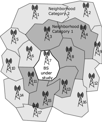
Figure 3: Example of neighborhood categories 1 and 2.

Note that in Fig. 3, BS 7 is the target of this analysis, and the BSs in neighborhood category 1 (dark gray) are part of the set of category 2 (light gray), as a consequence of Equation (9). To highlight the differences between the proposed neighboring structure and the classical geographical one, in this example, an immediate neighbor, such as BS $6$, is excluded from the neighborhood of category 1, and the more distant BS $4$ instead belongs to it. This choice is to emphasize the fact that distance is not the criterion to determine the membership of a neighborhood set, which is actually determined by the position in priority lists.

The u-v proximity

To find the set of neighbors for each target BS, we need to first compute the $u-v$ proximity. Two BSs have $u-v$ ($u<v$) proximity if there exists at least one device location such that in its priority list, the positions occupied by the two BSs are between the $u^{th}$ and $v^{th}$ positions (including the extremes).

Based on this definition, multiple $u-v$ proximities can be defined for a single pair of BS if there is more than one location whose list contains antennas from both BS. This occurs because a pair of BSs can occupy very diverse positions in the priority lists in different device locations. At a location well positioned to receive signals from both BSs, both might occupy the first two positions of the list. At a location far from both BSs, they might occupy the two last positions of the list.

The existence of multiple $u-v$ proximities for the same pair of BSs is not necessarily a problem. Their usefulness becomes evident when we consider that the signals from a single pair of BSs might not be received with enough strength in any device to have $1-2$ proximity, for example, but are received strongly enough in at least one device to have $2-3$ proximity. This allows us to say that these BSs do not belong to each other’s neighborhood category 1 but that they belong to each other’s neighborhood category 2. No device normally connected to one of them will have as a first choice the other BS in case of an access failure, unless there are two simultaneous failures.

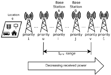
Figure 4: Range u-v of proximity between BSs (i,j).

We can formally define the $u-v$ range of priorities as the following ordered set:

$$\mathcal{I}_{u-v}=\{u,u+1,...,v\}$$ (11)

where $\xi\geq v>u\geq 1$.

Let the $u-v$ proximity indicator of a pair of BSs $b_{i},b_{j}\in\mathcal{B}$ be defined as follows:

$$P^{u-v}(b_{i},b_{j})=\begin{cases}1&\text{if }\exists g\in\mathcal{G}:\,\,b_{i},b_{j}\in\{b_{g,u},...,b_{g,v}\}\\ 0&\text{otherwise}\end{cases}$$ (12)

where

$i\neq j$;

$u,u+1,...,v\in\mathcal{I}_{u-v}$;

$b_{i},b_{j},\in\mathcal{B}$; and

$b_{g,u},...,b_{g,v}\in\mathbf{s}_{g}\subset\mathcal{B}$.

In Fig. 4, to visually show the $u-v$ proximity concept, the following are displayed: location $g\in\mathcal{G}$; the set of machines installed in $g$; and some of the $\xi$ BSs in the priority list $\mathbf{s}_{g}$. Note that, in this example, $u$, $i$, $j$, and $v$ all belong to the range $\mathcal{I}_{u-v}$. Therefore, applying the definition in (12), we have that $P^{u-v}(A,B)=1$, for BSs $A=b_{g,i}$ and $B=b_{g,j}$.

Note that the $u-v$ proximity is a symmetrical property, under the general assumption of the existence of at least one other location where the positions that both BSs occupy in a priority list are inverted. Therefore, for any pair of BSs $b_{i},b_{j}\in\mathcal{B}$, we have that:

$$P^{u-v}(b_{i},b_{j})=P^{u-v}(b_{j},b_{i}),\forall i\neq j$$ (13)

The $u-v$ proximity is a property that can be used to determine whether any pair of BSs has high, medium or low propensity of affecting each other’s performance by considering a $u-v$ range that covers positions at the beginning, middle or last part of the priority list. In our specific implementation, we are interested in identifying those BSs that belong to a specific neighborhood category. We can see in Equation (8) that the BSs of interest for a particular $\mathcal{C}^{n}$ are receiving traffic from the target BS with a probability of $p^{n-1}(1-p)$ or higher. This means that the $u-v$ range for this application starts in the first position ($u=1$).

TABLE II: Relation between priority, probability, category and proximity

Alternative	Position	$Pr$	Neighborhood	$u-v$
BSs	in $\mathbf{s}_{g}$		Categories	interval
$b_{g,2}$	2	$1(1-p)$	$\mathcal{C}^{1}$	$1-2$
$b_{g,3}$	3	$p(1-p)$	$\mathcal{C}^{2}$	$1-3$
$b_{g,4}$	4	$p^{2}(1-p)$	$\mathcal{C}^{3}$	$1-4$

Table II illustrates where the $u-v$ range ends, in relationship to a particular neighborhood category. We can observe the relationship between:

1. The position of the BSs in a priority list,

2. The probability they have of receiving access requests typically served by the BS in the first position if it fails,

3. The neighborhood of lowest category that includes each BS, and

4. the $u-v$ interval associated to each case.

Table II was built following the toy example presented in section IV-A to illustrate the intuition behind our approach, which was also used in Equation (IV-A). Under the assumption that $b_{g,1}$ fails, each of the three BSs has decreasing probabilities of receiving access requests originally intended for the BS in first position. We can appreciate as a general rule that for a neighborhood category $n$:

• BSs in positions $2,...,n+1$ are included in it.

• The lower bound of the probability these BSs have of receiving access requests from $b_{g,1}$ is $p^{n-1}(1-p)$.

• The associated proximity range ends in $n+1$.

We conclude that the $u-v$ range associated to a neighborhood category $n$ is $1-(n+1)$.

Formally:

$$b_{j\neq i}\in\mathcal{C}^{n}(b_{i})\Leftrightarrow P^{1-(n+1)}(b_{i},b_{j})=1$$ (14)

for at least one location $g\in\mathcal{G}$.

We can illustrate this relationship with the following example: if BS $b_{j}$ belongs to the neighborhood category $3$ of $b_{i}$ ($b_{j}\in\mathcal{C}^{3}(b_{i})$), it means that $b_{i}$ and $b_{j}$ have $1-4$ proximity ($P^{1-4}(b_{i},b_{j})=1$).

Because of the association defined between the notions of proximity and neighborhood, the symmetry defined in (13) also implies a symmetry in neighborhood relationships such that:

$$b_{j}\in\mathcal{C}^{n}(b_{i})\Leftrightarrow b_{i}\in\mathcal{C}^{n}(b_{j}),\forall i\neq j$$ (15)

Neighborhood matrices

In the proposed framework, we aggregate KPIs of the “neighbors” of a BS whose failing state we wish to study. To identify the neighbor BSs, we use a neighborhood indicator for each pair of BSs. We arrange these indicators in an $M\times M$ neighborhood matrix, where $M$ is the number of BSs in the system.

For a neighborhood category $n$, each element of the $M\times M$ neighborhood matrix $C^{n}$ is defined as:

$$c^{n}_{i,j}=\begin{cases}1&\text{if }b_{j}\in\mathcal{C}^{n}(b_{i}),j\neq i\\ 0&\text{otherwise}\end{cases}$$ (16)

Note that $c^{n}_{i,j}=0$ when $i=j$ and that $c^{n}_{i,j}=c^{n}_{j,i}$ because of (15).

The neighborhood matrices $C^{1}$ and $C^{5}$ computed in our implementation are partially shown in Figs. 5(a) and 5(b). We can observe that the BS identified with a $0$ is a neighbor of BSs $2$ and $4$ when considering a neighborhood of category $1$ (Fig. 5(a)). If we consider a neighborhood of category $5$, BS $0$ is also a neighbor of BS $5$. We can observe a similar situation for BSs $3$ and $5$, which have one more neighbor when the category is augmented to $5$. For the cellular network simulated, the matrices $C^{n}$ are of size $479\times 479$, as there are $479$ BSs in the city.

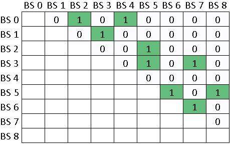
(a) Neighborhood category 1.

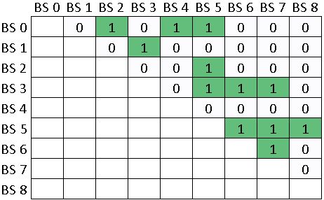
(b) Neighborhood category 5.

Figure 5: Example of neighborhood matrices.

The neighborhood matrices are computed once per cellular infrastructure and recomputed only if there is a change in the RSS values or if antennas or BSs are removed or added. The matrices are evaluated when aggregating the neighborhood KPIs for each of the BSs as part of the construction of the “feature vectors” that allow the use of ML for failure detection. As mentioned, a neighborhood is associated with the probability of experiencing a performance degradation as a consequence of a failure, whose pattern we intend to detect. The specifics on how KPIs are aggregated can be found in Section IV-C.

IV-B Network simulation

We use an LTE simulatorsimilar to the one described in [4]. The way IoT devices gain access to the BSs is based on the computation of priority lists ($\xi=12$) for each device served by the mobile infrastructure. The simulator allows for several propagation models to compute the RSS values involved in the construction of the priority lists. Because this model encompasses the uplink RACH procedure and the transmission until reception at the Evolved Packet Core (EPC), its output is composed of counters and statistics related to both phases:

• Number of packets created.

• Number of packets transmitted.

• Number of RACH collisions.

• Number of RACH attempts.

• Minima, maxima and average of the RACH delays.

• Minima, maxima and average of the transmission times (from RACH completion to reception at the EPC).

The priority lists are computed considering as options the antennas, instead of the BSs. In the preprocessing to compute the neighborhood matrices, the antennas identification codes in these lists is replaced by the identification of the BS where the antennas are installed.

The RACH failures are modeled as affecting simultaneously all the antennas of a particular BS. Because BSs generally do not have the same number of antennas, most of the time, the probabilities for the positions in the priority lists may have values higher than the theoretical minimum described in Section IV-A for a particular neighborhood category. We purposely choose to omit the implementation of countermeasures in the preprocessing to address the “noise” introduced by it, as the effect on the results does not hinder the methodology.

IV-B1 Simulated scenarios

In Table III, we show the devices types, levels of traffic, duration of the simulation, total number of BSs and number of failing BSs.

TABLE III: Simulation scenarios

Type of device	smart meters, surveillance cameras, bus stops, traffic lights, parking lots, microPMUs*
Levels of traffic	High / low
Simulation duration (h)	12
Total BSs	479
Failing BSs	50

• Micro-phasor measurement units are power monitoring devices.

We considered two scenarios in our simulations: high traffic and low traffic. In the high-traffic scenario, smart meters, parking slots, bus stops, surveillance cameras, and traffic lights generate packets at double rate with respect to the low-traffic scenario. Fire alarms and Micro-Phasor Measuring Units generated packets at the same rate for both scenarios.

IV-B2 RACH failure generation

In a random sample of 50 BSs, total RACH failures were parameterized to initiate at the beginning of each 1-hour simulation, with a duration of 30 minutes. This process was repeated 12 times (with different random seeds). In every simulation, the first 10 minutes are used to initialize the network and their results are omitted from the KPIs aggregation.

IV-C AN ML framework

IV-C1 Preprocessing

The output of the simulator was aggregated in three ways:

1. Across non-overlapping time-bins or intervals (according to the size of the time aggregations),

2. across the antennas of each BS, and

3. across the IoT devices.

As a result, the data set contained the statistics at the BS level and considered generic traffic (without distinction among the traffic generated by the different devices/applications). The results were preprocessed aggregating the data at the BS level in time intervals of 5, 10, 15 and 30 minutes. This allowed us to study the effect of aggregation size on detection performance.

A fundamental part of the preprocessing was the computation of the neighborhood matrices for each of the neighborhood categories. This process involves the following steps:

• Analyzing the priority lists for each location in the network.

• Processing the priority lists to obtain the $u-v$ proximities between each pair of BSs.

• Using the $u-v$ proximities to obtain the neighborhood matrices.

Our aggregating procedure consisted of computing the following statistics: average, variance, skewness, kurtosis, percentile (5, 25, 50, 75, 95), minimum, maximum and range.

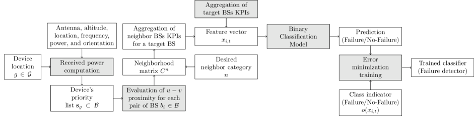
Figure 6: Graphical description of the proposed framework for failure detection.

After the data were aggregated for each interval/BS, a normalization step is used to force the values to lie within the range $(0,1)$.

The feature vectors ${x_{i,t}}$ to be used in the ML algorithms are built concatenating, for each aggregation interval $t$ and “target” BS $b_{i}$ two vectors:

• Aggregation of the statistics of BS $b_{i}$ during interval $t$.

• Aggregation of the statistics of all the neighboring BSs in $\mathcal{C}^{n}(b_{i})$ during interval $t$.

To perform supervised classification, the data set is completed by associating each feature vector $x_{i,t}$ to a category label, a class indicator or a “target value” $o(x_{i,t})$, defined as:

$$o(x_{i,t})=\begin{cases}1&\text{if }f(b_{i})=1\text{ at interval }t\\ 0&\text{otherwise}\end{cases}$$ (17)

This procedure is repeated using the data generated by the simulator for each time aggregation size and neighborhood category. The whole process, for a particular interval of time, is described in the diagram in Fig. 6.

IV-C2 Models and training strategy

We report our results for the following binary classifiers:

1. Naive Bayes

2. Logistic Regression

3. Linear, Quadratic, Cubic and Radial Basis Function (RBF) Support Vector Machines

4. Decision Trees

5. Extra Trees

6. Bagged Decision Trees

7. Random Forest

8. Shallow (Single Hidden Layer) Neural Networks

For each of the simulation scenarios and preprocessing strategies, the data set is randomly split into training ($70\%$) and testing ($30\%$) sets. Parameter tuning for each of the classification models is performed via $10$-fold cross-validation (within the data from the training set).

The detection (classification) performance was mainly evaluated via the ROC AUC score. However, failure investigation activities associated with a false alarm represent a considerable operational cost for telco providers. Consequently, we also computed the FPRs as a performance index.

In Fig. 6, we explain the ML framework for failure detection. Notice that gray boxes represent processes or actions and that white boxes represent their products, intermediate products or inputs. The process starts with the RSS measurements, by probing in a deployed network or by simulation. In our implementation, RSS values were computed for each antenna in each location $g\in\mathcal{G}$ and used to construct the priority lists $\mathbf{s}_{g}$. After the lists were created, each pair of BSs was considered one at a time, and the list of each location was checked to see if it contained the pair of BSs and in which positions of priority. By observing these positions, a practitioner could compute each of the $u-v$ proximities for the pair of BSs. Once the practitioner decided which neighborhood category to consider, $u-v$ proximities of each pair of BSs can be used to determine whether or not they are neighbors. When the feature vector was built for a specific target BS, the KPIs vectors of its neighbors were concatenated to the KPIs vector of the target BS. The process was repeated for all the BSs, for all the time intervals under study, to build the data set. Then, the training process took place by minimizing some norm of the difference between the prediction and the real target value. The target value was obtained from the simulation parameters. If there was an ongoing failure in the BS in a specific interval, the target value was defined as 1. Otherwise, the target value was 0.

IV-D Implementation and scalability details

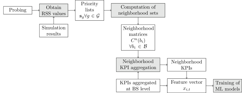
Figure 7: Implementation process.

The proposed framework is based on four main processes (see Fig. 7):

1. Retrieval of RSS values at each potential device location and creation of priority lists.

2. Computation of neighborhood sets based on the priority lists.

3. Data aggregation (both at the BS level and of neighborhoods based on the neighborhood matrices).

4. Training and evaluation of ML models using the aggregated data.

The real-world application of the framework requires some efforts from an operator:

1. RSS retrieval is a process that can be done via probing a deployed network at each of the potential IoT device locations or via simulation of the BSs’ signal propagation.

2. Neighborhood computation requires finding the $u-v$ proximities for each pair of BSs and the further creation of neighborhood sets for each neighborhood category.

3. Data aggregation.

4. All the MLs models to be trained and evaluated are well-known models, whose complexities and difficulties are well known, and there exists a plethora of pipe-line design strategies that can be used.

In what follows, the first two operator’s challenges are analyzed.

To obtain the RSS measurements, the telco operator would first need to identify the potential IoT device locations and undertake a project to probe, at each location, the signal strength of the BSs in the range of each location. An alternative approach would be to use simulations, as in this work. Instead of considering only the potential locations for devices, we divided the space of the city into a grid of squares. The positions of the IoT devices inside a grid square are approximated with the center of the grid square. The RSS of every antenna of every BS in the simulated network was computed taking into account the antenna tilt, orientation and power, as well as distances and frequencies.

The outcome of this simulation is a data structure of length $\xi G$ (worst-case scenario), where $G$ is the total number of squares in the grid and $\xi$ is the size of the priority lists of antennas at each square. Each item in the structure is a vector containing information regarding the location of the square, the identification of both the BS and the antenna and the RSS value.

Another important implementation task is the computation of the neighborhood matrices. To study the scalability of this process so that an operator can estimate its feasibility, we show the computational complexity associated with the process. Assuming that $M$ is the total number of BSs in the city, the computational complexity of the procedure is given by the following polynomial expression:

$$O(M^{2}+G)$$ (18)

A distance-based approach, in contrast, involves the computation of the Voronoi regions around each of the BSs, a process the computational complexity of which is, in general [33]:

$$O(M\log{M})$$ (19)

Compared to Equation (19), the complexity of the neighborhood matrices can be considered more computationally expensive. However, being polynomial, the method can be considered scalable. If the number $M$ of BSs of the network is considered constant, Equation (18) becomes $O(G)$, which is linear with respect to the number $G$ of potential IoT device locations.

V Numerical results

TABLE IV: Minimum and average ROC AUC for each classifier.

	ROC AUC
Classification model	Average	Minimum
Extra Trees	0.997	0.971
Random Forests	0.985	0.921
Decision Trees	0.984	0.897
Naive Bayes	0.983	0.938
Bagged Decision Trees	0.981	0.879
Linear Support Vector Machine (SVM)	0.959	0.912
Shallow Neural Network	0.955	0.898
Quadratic SVM	0.954	0.891
Logistic Regression	0.954	0.877
RBF SVM	0.953	0.902
Cubic SVM	0.952	0.875

We now discuss the results obtained after using four classifiers in the following task: to determine if a specific vector of aggregated KPIs taken during a time interval at a specific BS was produced or not during an ongoing failure. This was achieved without knowledge of the past behavior of the BS.

According to their classification performance both from the point of view of the ROC AUC and FPR, in all of our experiments, we could identify two groups of supervised classifiers:

• Group 1: consisting of all the SVM classifiers, along with Logistic Regressions and the Shallow Neural Networks, which achieve on average an AUC score below $0.981$.

• Group 2: consisting of the ensemble learners (Bagged Decision Trees, Random Forests and Extra Trees), Decision Trees and Naive Bayes, the average AUC of which is higher than $0.98$. The Extra Trees classifiers in particular, in the worst performance, achieved an AUC higher than $0.97$, and the average score was above $0.99$. We indicate the classifiers of this group with italics in Table IV.

The behavior of the performance of these groups is shown in Figs. 8, 10, and 9. It can be argued that the pattern is easily separable, as a low-complexity classifier like Naive Bayes performs very well. While Extra Trees is not a simple classifier, its building strategy is less prone to overfitting than traditional one-hidden-layer Neural Networks and kernel-based methods (SVMs), which might explain its dominance over those models.

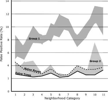
Figure 8: Effect of neighborhood category on false positive rate per classifier.

It is important to keep in mind that these AUC and FPR values are obtained without any BS-related information (BS ID, time, coordinates, number of devices producing traffic, application types, etc).

Among all the experiments, the average effect of increasing the traffic intensity is mild (never higher than $1\%$), though in most classifiers, the effect is slightly negative. Extra Trees is an exception, showing a slightly positive average reaction.

V-A Effect of neighborhood category

In Fig. 8 we show the FPR observed when applying the classification models on the 11 data sets generated by aggregating the simulated data considering the 11 neighborhood matrices (for categories $1,...,11$). The reader should note that the neighborhood definition affects which (and how many) BSs’ KPIs are included to detect the failure. The FPR computed for each classifier in this graph is the average of the FPRs obtained under the two traffic levels for each of the time aggregation sizes, to observe only the effect of the change in the neighborhood definition.

It is notable that, in general, increasing the category of the neighborhood definition has a detrimental effect on the FPR values for classifiers of group 1. The FPR values for classifiers of group 2, on the other hand, exhibit neither a clear improvement nor a clear deterioration when increasing the size of the neighborhoods considered. The results suggest that there is no justification for using neighborhoods of categories higher than 3 when considering FPRs values.

In Fig. 9, we observe the response of the ROC AUC values with respect to changes in the neighborhood definition. A clear distinction in the behavior of classifiers of Groups 1 and 2 can also be observed in terms of the AUC, and group 2 does not appear to benefit from having a neighborhood category higher than 3. The performance of classification models in group 1 also deteriorates in terms of the AUC, progressively losing the separation ability as the neighborhood size increases.

V-B Effect of aggregation size

In Fig. 10, we show how the average ROC AUC values for each group of classifiers responds to increasing sizes of the aggregation time bins. To build this figure, we averaged the AUC values obtained by each classifier over the data generated under the two levels of traffic and preprocessed under the 11 neighborhood categories to observe only the effect produced by the size of the aggregation bins.

We find that increasing aggregation size from 5 to 10 minutes has effects that range from mild (for classifiers of Group 2, which already have AUC values higher than $0.97$) to clearly positive (for classifiers of Group 1) (see Fig. 10). With the exception of Bagged Trees, all models in Group 2 clearly benefit from the increase in aggregation from 10 to 15 minutes. Increasing the aggregation to 30 minutes, however, appears to blur the patterns and provoke a deterioration of their performance. Models of Group 1 had no performance improvement when augmenting the aggregation size to 15 minutes and had no uniform response to the increase in aggregation size to 30 minutes.

When averaging to observe the ROC AUC and FPR responses to all the neighborhood categories and all the aggregations sizes, Extra Trees consistently showed the best performance. Naive Bayes, being a less complex classifier, had similar results on average, and might be a sound enough choice for an operator in the scenarios at hand.

V-C Interaction between aggregation size and neighborhood category

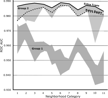
Figure 9: Effect of neighborhood category on AUC for each classifier.

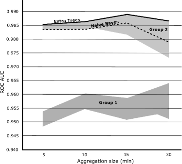
Figure 10: Effect of aggregation on AUC for each classifier.

Figs. 11 and 12 show the average AUC scores for the two best models: Extra Trees and Naive Bayes, respectively. In these figures, to analyze the joint effect of time aggregation size and neighborhood category, we created a heatmap, in which lighter colors represent higher AUC scores and consequently better detection performance.

To compute these values, the AUC values were averaged among only the two traffic levels to observe the interaction between the neighborhood definition and time aggregation.

In the aforementioned figures, it can be noted that both methods produced AUC scores close to 1, making evident that the models have a high separation capacity for these data sets. However, neighborhood categories 2, 3 and 4 obtained the best scores, especially when the size of the time aggregations was 10, 15 and 30.

In particular, the best results were achieved with 15 minutes of aggregation and neighborhood category 2, allowing the Extra Trees classifiers to achieve an AUC score of $0.996$, and the Naive Bayes classifier a score of $0.993$.

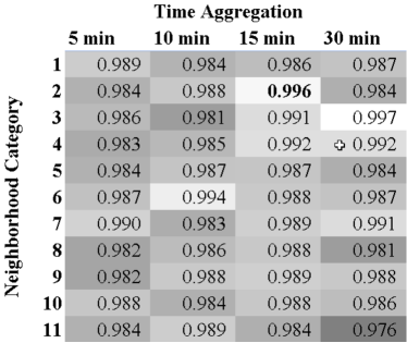
Figure 11: Joint effect of proximity and aggregation levels on Extra Trees AUC score.

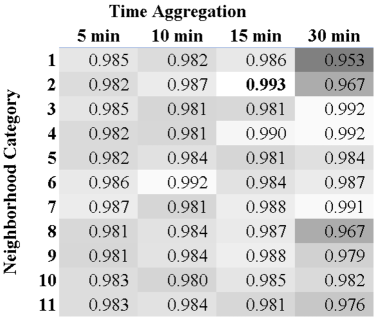
Figure 12: Joint effect of proximity and aggregation levels on Naive Bayes AUC score.

VI Conclusions and future work

In this paper, we proposed a supervised learning framework to detect RACH-related sleeping cells in a smart-city cellular infrastructure. We used well-known binary classification techniques to detect network elements at fault based on the analysis of aggregated KPIs such as the RACH collision probability and the delay.

RACH-related sleeping cells are difficult to detect due to the lack of evidence in the KPIs from a faulty cell. To overcome this problem, we have proposed to jointly consider the KPIs of one cell with those from the neighboring cells. We have also proposed a novel definition for neighbors of a cell, not choosing the nodes geographically closer to a cell but rather those that would be more likely impacted by its failure.

We used data obtained from a large-scale IoT network simulator that employs real data on the telecommunication infrastructure and on the position of IoT nodes in a smart-city environment. Although LTE was chosen to obtain numerical results, the proposed framework can easily be adapted to other cellular technologies, such as 5G.

Different time aggregation interval sizes were tested for the KPIs: 15 minutes resulted in the aggregation interval that permitted achieving the highest AUC. This aggregation level permits heavily reducing the amount of data to be analyzed by a network operator to detect faulty elements, resulting in large potential savings. The numerical results also proved Extra Trees and Naive Bayes to be the most effective binary classification techniques among the ones considered in this work. Broadly speaking, the results suggest that simple and ensemble models, known for being less prone to overfitting, are superior to kernel models and neural networks.

The preprocessing approach based on aggregations and the inclusion of information regarding the “neighborhood” of a BS has shown its value in the classification task. We are currently working on how to adapt this strategy for forecasting and anomaly detection.

Orestes G. Manzanilla-Salazar (M’19) received his B.S. (2002) in production engineering and his M.S. (2005) in systems engineering from Simón Bolívar University (USB) in Venezuela. He is currently working on his Ph.D in electrical engineering at Ecole Polytechnique de Montreal, Montreal, QC, Canada. From 2008 to 2015, he was an Assistant Lecturer at USB. He taught courses in the areas of mathematical programming, decision science and operations management and focused his research on linear and integer programming models to create supervised classifiers. He worked 6 years in several positions for private firms in the areas of engineering, technology and finance. His present research focus is on machine learning and analytics tools for telco networks management and on network-enabled systems.

Filippo Malandra (M’17) received B.Eng. and M.Eng. degrees in telecommunications engineering from the Politecnico di Milano, Milan, in 2008 and 2011, respectively, and a Ph.D. degree in electrical engineering from Ecole Polytechnique de Montreal, Montreal, QC, Canada, in 2016. He is currently an Assistant Professor of Research with the Department of Electrical Engineering at the University at Buffalo. His research interests include the performance analysis and simulation of mobile networks (4G/5G) for smart grids, smart cities and IoT applications.

Hakim Mellah received his B.S (1996) and M.Sc.(1999) in electrical engineering and his Ph.D. in electrical and computer engineering from Concordia University, Montreal, QC, Canada, in 2018. He is currently a postdoc at Ecole Polytechnique de Montreal. His research interests focus mainly on machine quality of experience for IoT applications in a smart-city environment.

Constant Wette holds an M.Sc. in computer engineering from Ecole Polytechnique de Montreal, Montreal, QC, Canada (2000), an M.Eng. in electrical engineering from Ecole Polytechnique de Yaoundé, Cameroon (1996), an MBA from HEC Montreal, Montreal, QC, Canada (2010) and a Graduate Certificate in data science from Harvard University (2016). He is a Senior System Developer at Business Area Digital Services, Ericsson. He joined Ericsson in 2000 and has led research projects, product development, innovation and new business development in different technology domains including data analytics, IoT/M2M, IMS and telecommunication cloud architectures.

Brunilde Sansò (M’92–SM’17) is a Full Professor of telecommunication networks with the Department of Electrical Engineering, Ecole Polytechnique de Montreal, and the Director of the LORLAB, a research group dedicated to developing methods for the design and performance of wireless and wireline telecommunication networks. Over her career of more than 25 years, she has received several awards and honors, has published extensively in the telecommunication networks and operations research literature, and has been a consultant for telecommunication operators, equipment and software manufacturers, and the mainstream media.

References

- [1] J. Jin, J. Gubbi, S. Marusic, and M. Palaniswami, “An information framework for creating a smart city through internet of things,” IEEE Internet of Things journal, vol. 1, no. 2, pp. 112–121, 2014.
- [2] A. Zanella, N. Bui, A. Castellani, L. Vangelista, and M. Zorzi, “Internet of things for smart cities,” IEEE Internet of Things journal, vol. 1, no. 1, pp. 22–32, 2014.
- [3] J. Lin, W. Yu, N. Zhang, X. Yang, H. Zhang, and W. Zhao, “A survey on internet of things: Architecture, enabling technologies, security and privacy, and applications,” IEEE Internet of Things Journal, vol. 4, no. 5, pp. 1125–1142, 2017.
- [4] F. Malandra, L. Chiquette, L.-P. Lafontaine-Bédard, and B. Sansò, “Traffic characterization and LTE performance analysis for M2M communications in smart cities,” Pervasive and Mobile Computing, no. 48, pp. 59–68, 2018.
- [5] R. Barco, P. Lazaro, and P. Munoz, “A unified framework for self-healing in wireless networks,” IEEE Communications Magazine, vol. 50, no. 12, 2012.
- [6] M. Polese, M. Centenaro, A. Zanella, and M. Zorzi, “M2M massive access in lte: Rach performance evaluation in a smart city scenario,” in 2016 IEEE International Conference on Communications (ICC). IEEE, 2016, pp. 1–6.
- [7] A. Coluccia, A. D’Alconzo, and F. Ricciato, “Distribution-based anomaly detection via generalized likelihood ratio test: A general maximum entropy approach,” Computer Networks, vol. 57, no. 17, pp. 3446–3462, 2013.
- [8] M. Z. Shafiq, L. Ji, A. X. Liu, J. Pang, and J. Wang, “A first look at cellular machine-to-machine traffic: large scale measurement and characterization,” in ACM SIGMETRICS Performance Evaluation Review, vol. 40. ACM, 2012, Conference Proceedings, pp. 65–76.
- [9] ——, “Large-scale measurement and characterization of cellular machine-to-machine traffic,” Networking, IEEE/ACM Transactions on, vol. 21, no. 6, pp. 1960–1973, 2013.
- [10] I. de-la Bandera, R. Barco, P. Munoz, and I. Serrano, “Cell outage detection based on handover statistics,” IEEE Communications Letters, vol. 19, no. 7, pp. 1189–1192, 2015.
- [11] S. Rezaei, H. Radmanesh, P. Alavizadeh, H. Nikoofar, and F. Lahouti, “Automatic fault detection and diagnosis in cellular networks using operations support systems data,” in Network Operations and Management Symposium (NOMS), 2016 IEEE/IFIP. IEEE, 2016, pp. 468–473.
- [12] R. M. Khanafer, B. Solana, J. Triola, R. Barco, L. Moltsen, Z. Altman, and P. Lazaro, “Automated diagnosis for UMTS networks using Bayesian network approach,” IEEE Transactions on vehicular technology, vol. 57, no. 4, pp. 2451–2461, 2008.
- [13] C. M. Mueller, M. Kaschub, C. Blankenhorn, and S. Wanke, “A cell outage detection algorithm using neighbor cell list reports,” in International Workshop on Self-Organizing Systems. Springer, 2008, pp. 218–229.
- [14] F. Chernogorov, J. Turkka, T. Ristaniemi, and A. Averbuch, “Detection of sleeping cells in lte networks using diffusion maps,” in Vehicular Technology Conference (VTC Spring), 2011 IEEE 73rd. IEEE, 2011, pp. 1–5.
- [15] M. Panda and P. M. Khilar, “Distributed soft fault detection algorithm in wireless sensor networks using statistical test,” in 2012 2nd IEEE International Conference on Parallel, Distributed and Grid Computing. IEEE, 2012, pp. 195–198.
- [16] Y. Ma, M. Peng, W. Xue, and X. Ji, “A dynamic affinity propagation clustering algorithm for cell outage detection in self-healing networks,” in Wireless Communications and Networking Conference (WCNC), 2013 IEEE. IEEE, 2013, pp. 2266–2270.
- [17] A. Gómez-Andrades, P. Muñoz, E. J. Khatib, I. de-la Bandera, I. Serrano, and R. Barco, “Methodology for the design and evaluation of self-healing LTE networks,” IEEE Transactions on Vehicular Technology, vol. 65, no. 8, pp. 6468–6486, 2015.
- [18] M. Sun, H. Qian, K. Zhu, D. Guan, and R. Wang, “Ensemble learning and smote based fault diagnosis system in self-organizing cellular networks,” in GLOBECOM 2017-2017 IEEE Global Communications Conference. IEEE, 2017, pp. 1–6.
- [19] O. Manzanilla-Salazar, F. Malandra, and B. Sansò, “eNodeB failure detection from aggregated performance KPIs in smart-city LTE infrastructures,” in 15th International Conference on the Design of Reliable Communication Networks, DRCN 2019, Coimbra, Portugal, March 19-21, 2019, 2019, pp. 51–58.
- [20] E. J. Khatib, R. Barco, A. Gómez-Andrades, P. Muñoz, and I. Serrano, “Data mining for fuzzy diagnosis systems in LTE networks,” Expert Systems with Applications, vol. 42, no. 21, pp. 7549–7559, 2015.
- [21] “Smart cities M2M traffic characterization and performance analysis,” https://www.trafficm2modelling.com/home, accessed: 2019-02-01.
- [22] H. Zhang, Y. Ren, K.-C. Chen, L. Hanzo et al., “Thirty years of machine learning: The road to pareto-optimal next-generation wireless networks,” arXiv preprint arXiv:1902.01946, 2019.
- [23] B. Cheung, S. Fishkin, G. Kumar, and S. Rao, “Method of monitoring wireless network performance,” Mar. 23 2006, uS Patent App. 10/946,255.
- [24] Q. Liao, M. Wiczanowski, and S. Stańczak, “Toward cell outage detection with composite hypothesis testing,” in Communications (ICC), 2012 IEEE International Conference on. IEEE, 2012, pp. 4883–4887.
- [25] F. Chernogorov, S. Chernov, K. Brigatti, and T. Ristaniemi, “Sequence-based detection of sleeping cell failures in mobile networks,” Wireless Networks, vol. 22, no. 6, pp. 2029–2048, 2016.
- [26] A. Gómez-Andrades, P. Muñoz, I. Serrano, and R. Barco, “Automatic root cause analysis for LTE networks based on unsupervised techniques,” IEEE Transactions on Vehicular Technology, vol. 65, no. 4, pp. 2369–2386, 2016.
- [27] X. Liu, G. Chuai, W. Gao, and K. Zhang, “GA-AdaBoostSVM classifier empowered wireless network diagnosis,” EURASIP Journal on Wireless Communications and Networking, vol. 2018, no. 1, p. 77, 2018.
- [28] E. J. Khatib, R. Barco, P. Muñoz, and I. Serrano, “Knowledge acquisition for fault management in LTE networks,” Wireless Personal Communications, vol. 95, no. 3, pp. 2895–2914, 2017.
- [29] F. Malandra, P. Potvin, S. Rochefort, and B. Sansò, “A case study for M2M traffic characterization in a smart city environment,” in International Conference on Internet of Things and Machine Learning (IML 2017), Liverpool, UK, Oct. 2017, pp. 1–9.
- [30] “Spectrum management system data,” https://sms-sgs.ic.gc.ca/eic/site/sms-sgs-prod.nsf/eng/h_00010.html, accessed: 2019-09-09.
- [31] R. V. Akhpashev and A. V. Andreev, “Cost 231 hata adaptation model for urban conditions in lte networks,” in 2016 17th International Conference of Young Specialists on Micro/Nanotechnologies and Electron Devices (EDM), June 2016, pp. 64–66.
- [32] S. Hämäläinen, H. Sanneck, and C. Sartori, LTE self-organising networks (SON): network management automation for operational efficiency. John Wiley & Sons, 2012.
- [33] F. Aurenhammer, “Voronoi diagrams—a survey of a fundamental geometric data structure,” ACM Computing Surveys (CSUR), vol. 23, no. 3, pp. 345–405, 1991.