Right-sizing fluxonium against charge noise

Abstract

We analyze the charge-noise induced coherence time $T_{2}$ of the fluxonium qubit as a function of the number of array junctions in the device, $N$. The pure dephasing rate decreases with $N$, but we find that the relaxation rate increases, so $T_{2}$ achieves an optimum as a function of $N$. This optimum can be much smaller than the number typically chosen in experiments, yielding a route to improved fluxonium coherence and simplified device fabrication at the same time.

Introduction—

One of the earliest superconducting qubits was the Cooper-pair box Shnirman et al. (1997); Bouchiat et al. (1998); Nakamura et al. (1999). This qubit design is intuitive, with the $\left|0\right>$ and $\left|1\right>$ states corresponding physically to an excess Cooper-pair residing on or off a small superconducting island. However, it did not take long before experiments demonstrated its acute vulnerability to ambient charge noise Nakamura et al. (2002). One popular modification of the Cooper-pair box is the transmon qubit Koch et al. (2007), which adds a capacitive shunt to increase robustness against charge noise at the cost of reduced spectral anharmonicity. The superconducting flux qubit Orlando et al. (1999) offers an alternative that can exhibit large anharmonicity, and researchers continue to refine its design Yan et al. (2016). One innovative reconsideration of the flux qubit, called ”fluxonium,” was proposed Manucharyan et al. (2009) to suppress charge-noise sensitivity in all of the eigenstates of the system. In this paper, we present a potent optimization of the fluxonium design that minimizes its charge-noise decoherence.

Fluxonium exploits the fact that a single piece of metal naturally keeps its voltage uniform even in the presence of static external electric fields. So, instead of a standard flux qubit comprised of three or four superconducting islands, one imagines a qubit constructed from a single, annulus-shaped, island. The annulus is interrupted by a Josephson junction, and the body of the annulus shunts that junction with a large inductance, as in Fig. 1a. Since it is made of a single island of metal, such a qubit should remain indifferent to low-frequency charge noise.

In practice, the inductance of such a loop is too small to permit a good qubit. To produce the required large inductance, fluxonium adds a long chain of islands to the loop Manucharyan et al. (2009), strongly coupled via Josephson junctions, as in Fig. 1b. This design choice requires deliberation – our qubit was motivated by the robustness of a continuous piece of metal, so it seems counterproductive to incorporate a large number of islands. In the following, we confirm that, as long as the islands are coupled together sufficiently strongly, they can behave like a single piece of superconductor as far as low-frequency charge noise is concerned. However, using a standard model of charge noise Yan et al. (2016), we show that the qubit relaxation rate scales with the number of islands. This leads to our main result: for given fluxonium qubit parameters, there is an optimal number of islands that maximizes the qubit’s decoherence time $T_{2}$. We focus here on the original fluxonium proposal Manucharyan et al. (2009) in which the inductor is formed by a chain of coupled superconducting islands, but our findings may be relevant for alternative realizations of the inductor Hazard et al. (2019); Grünhaupt et al. (2019); Niepce et al. (2019) provided they can be modeled Matveev et al. (2002); Maleeva et al. (2018) by such a chain.

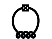
(a)

(b)

Figure 1: The fluxonium qubit. LABEL:sub@Fig:Cartoon Sketch of fluxonium. Single island of superconductor is interrupted by a single Josephson junction. The body of the island carries an inductance. LABEL:sub@Fig:circuit Fluxonium circuit diagram. A “black-sheep” junction Manucharyan et al. (2012) with Josephson energy $E_{J}^{b}$ and capacitance $C^{b}$ is shunted by an array of junctions with Josephson energy $E_{J}^{a}$ and capacitance $C^{a}$. To model dissipation (circuit elements in red), the superconducting array islands and the end islands are coupled to ground via capacitances $C^{a}_{d}$ and $C^{b}_{d}$ respectively. An impedance, placed in series with each ground capacitor, causes its voltage drop to fluctuate Devoret (1997). This models ambient charge noise.

Hamiltonian —

To calculate the charge-noise decoherence rate of fluxonium, consider the superconducting circuit depicted in Fig. 1b. The loop is pierced by time-independent flux $\Phi$, so that $\varphi\equiv 2e\Phi/\hbar$ is dimensionless. We have labelled the gauge-invariant phase drops as shown. The Lagrangian associated with this circuit is $\mathcal{L}=\mathcal{T}+\mathcal{T}_{d}-\mathcal{U}$. Here, the Josephson energy is

$$\mathcal{U}=E_{J}^{a}\sum_{i=1}^{N}(1-\cos\Theta_{i})+E_{J}^{b}(1-\cos(\sum_{i=1}^{N}\Theta_{i}-\varphi).$$ (1)

The capacitative energy is composed of two parts. The first describes the capacitors around the superconducting loop,

$$\mathcal{T}=\frac{1}{2}C^{a}\sum_{i=1}^{N}\left(\frac{\hbar\dot{\Theta}_{i}}{2e}\right)^{2}+\frac{1}{2}C^{b}\left(\sum_{i=1}^{N}\frac{\hbar\dot{\Theta}_{i}}{2e}\right)^{2}.$$ (2)

The second part, $\mathcal{T}_{d}$, describes capacitive coupling to dissipative elements. These dissipative elements, modeled as impedances Devoret (1997); Caldeira and Leggett (1983), are shown in red in Fig. 1b. Placed in series with small capacitances to ground $C_{d}^{a}$ and $C_{d}^{b}$, they produce voltage fluctuations $V_{i}$ that model background charge noise Yan et al. (2016). The associated energy is

$$\begin{split}&{\cal T}_{d}=\sum_{i=1}^{N-1}\frac{1}{2}C_{d}^{a}\Big{(}\frac{\hbar\dot{\tau}}{2e}+\sum_{j=1}^{i}\frac{\hbar\dot{\Theta}_{j}}{2e}-V_{i}\Big{)}^{2}\\ &+\frac{1}{2}C_{d}^{b}\Big{(}\frac{\hbar\dot{\tau}}{2e}-V_{0}\Big{)}^{2}+\frac{1}{2}C_{d}^{b}\Big{(}\frac{\hbar\dot{\tau}}{2e}+\sum_{j=1}^{N}\frac{\hbar\dot{\Theta}_{j}}{2e}-V_{N}\Big{)}^{2}.\end{split}$$ (3)

We define (dimensionless) canonical momenta $\mathcal{N}_{\tau}=\partial\mathcal{L}/\partial\hbar\dot{\tau}$ and $\mathcal{N}_{i}=\partial\mathcal{L}/\partial\hbar\dot{\Theta}_{i}$. Physically, the $\mathcal{N}_{i}$ are integer-valued variables determined by the number of Cooper pairs residing on islands of the circuit. A standard Legendre transformation yields the Hamiltonian

$$\mathcal{H}=\frac{1}{2}\left[\begin{array}[]{c}2e\mathcal{N}_{\tau}+Q_{\tau}\\ 2e\mathcal{N}_{1}+Q_{1}\\ \vdots\\ 2e\mathcal{N}_{N}+Q_{N}\end{array}\right]^{T}{\cal C}^{-1}\left[\begin{array}[]{c}2e\mathcal{N}_{\tau}+Q_{\tau}\\ 2e\mathcal{N}_{1}+Q_{1}\\ \vdots\\ 2e\mathcal{N}_{N}+Q_{N}\end{array}\right]+{\cal U}$$ (4)

where $\mathcal{C}$ is the capacitance matrix obtained from Eqs. 2 and 3 and the offset charges have the form

$$Q_{i}=C_{d}^{a}\sum_{j=i}^{N-1}V_{j}+C_{d}^{b}V_{N}\,\,\,\,\,\,\text{ and }\,\,\,\,\,\,\,Q_{\tau}=C_{d}^{b}V_{0}+Q_{1}.$$ (5)

The fact that (5) involves sums of voltages leads to larger offset charge fluctuations than one might naively assume. This plays a central role in making the fluxonium relaxation rate increase with $N$ as we show below.

To analyze $\mathcal{H}$, first note Ferguson et al. (2013) that $\mathcal{N}_{\tau}$ is a conserved quantity since $\tau$ is absent from the Josephson energy $\mathcal{U}$. We can therefore set $\mathcal{N}_{\tau}$ to zero in $\mathcal{H}$, restricting our attention to eigenstates of $\mathcal{H}$ that are independent of $\tau$.

Next, we specialize to the case of large $E_{J}^{a}$, which is suitable for fluxonium Manucharyan et al. (2009). The low-energy eigenstates then reside in the region $\Theta_{i}\ll 1$, and we approximate $\cos\Theta_{i}\approx 1-\Theta_{i}^{2}/2$. This renders the Hamiltonian mostly harmonic. Following the usual procedure for harmonic Hamiltonians, we introduce a real unitary (orthogonal) transformation $U$ to define $N$ new variables $n_{i}=\sum_{j=1}^{N}U_{ij}\mathcal{N}_{j}$, $q_{i}=\sum_{j=1}^{N}U_{ij}Q_{j}$, and $\theta_{i}=\sum_{j=1}^{N}U_{ij}\Theta_{j}$. We set $U_{1j}=1/\sqrt{N}$, so that $\theta_{1}=\sum_{j=1}^{N}\Theta_{j}/\sqrt{N}$ is an equal superposition mode. Then, the Hamiltonian decomposes to $\mathcal{H}_{\rm eff}=\sum_{i=1}^{N}H_{i}$, where

$$\begin{split}H_{1}&=\frac{\left(2en_{1}+q_{1}-\sqrt{N}Q_{\tau}/2\right)^{2}}{2(C^{a}+NC^{b})}\\ &+\frac{E_{J}^{a}}{2}\theta_{1}^{2}+E_{J}^{b}(1-\cos(\sqrt{N}\theta_{1}-\varphi)),\end{split}$$ (6)

$$H_{i\neq 1}=4E_{C}^{a}(n_{i}+\frac{q_{i}}{2e})^{2}+\frac{1}{2}E_{J}^{a}\theta_{i}^{2}.$$ (7)

Here, we have neglected the effect of $C_{d}^{a}$ and $C_{d}^{b}$ on the capacitance denominators and have defined $E_{C}^{a}=e^{2}/2C^{a}$.

The form of $H_{1}$ becomes more familiar if we set ${\theta=\sqrt{N}\theta_{1}}$, ${n=n_{1}/\sqrt{N}}$, ${q=q_{1}/\sqrt{N}-Q_{\tau}/2}$. Then,

$$H_{1}=4E_{C}\left(n+\frac{q}{2e}\right)^{2}+E_{J}(1-\cos(\theta-\varphi))+\frac{E_{L}\theta^{2}}{2},$$ (8)

where $E_{C}=e^{2}/2(C^{a}/N+C^{b})$, $E_{J}=E_{J}^{b}$, and ${E_{L}=E_{J}^{a}/N}$. These effective parameters determine the physics of the qubit. Keeping them fixed, the same Hamiltonian (8) can be realized for different $N$ provided the array junction parameters vary as $C^{a}=N(e^{2}/2E_{C}-C^{b})$ and $E_{J}^{a}=NE_{L}$. Physically, $C^{a}$ and $E_{J}^{a}$ can be tuned this way by simply changing the area of the array junctions. The central problem we address in this paper is to optimize the charge-noise robustness of fluxonium as a function of $N$.

To make the dependence on $N$ explicit, we rewrite Eq. 7 as

$$H_{i\neq 1}=\frac{4}{N}\mathcal{E}_{C}^{a}(n_{i}+\frac{q_{i}}{2e})^{2}+\frac{NE_{L}}{2}\theta_{i}^{2}$$ (9)

with $\mathcal{E}_{C}^{a}\equiv NE_{C}^{a}=1/(1/E_{C}-2C^{b}/e^{2})$ independent of $N$.

Approximate solution—

The approximate Hamiltonian $\mathcal{H}_{\text{eff}}$ is conveniently separated in terms of the new variables $\theta,\theta_{2},\dots,\theta_{N}$, so we can find the eigenstates of each term individually. We denote the Gaussian ground state of the Hamiltonian (9) by $e^{-i\theta_{i}q_{i}/2e}\phi_{0}(\theta)$, and the ground state and first excited state of Eq. 8 by $e^{-i\theta q/2e}\psi_{0}(\theta)$ and $e^{-i\theta q/2e}\psi_{1}(\theta)$, respectively. These states satisfy the usual boundary conditions, vanishing as $\theta\rightarrow\pm\infty$.

At first, it appears that the exact ground state of $\mathcal{H}_{\text{eff}}$ is

$$\begin{split}\chi_{0}&(\theta,\{\theta_{i}\})=e^{-i(q\theta+\sum_{i=2}^{N}q_{i}\theta_{i})/2e}\psi_{0}(\theta)\prod_{j=2}^{N}\phi_{0}(\theta_{j}).\end{split}$$ (10)

The phase factor in front removes the background charges from $\mathcal{H}_{\text{eff}}$, so that its ground state energy is perfectly independent of low-frequency charge noise. In fact, this phase factor can be placed in front of every eigenstate of $\mathcal{H}_{\text{eff}}$, so the entire energy spectrum seems to be independent of low-frequency charge noise, the goal described in the second paragraph of this paper.

Upon reflection, we realize that $\chi_{0}$ unfortunately does not satisfy the correct boundary conditions. Physically, each superconducting island of the circuit must house an integral number of Cooper pairs. It follows that $\Theta_{i}$, since it is conjugate to the discrete variable $\mathcal{N}_{i}$, must be a compact variable. In other words, changing the value of $\Theta_{i}$ by $2\pi$ does not describe a different state of the system, so the quantum mechanical wavefunctions of the circuit must satisfy periodic boundary conditions in $\Theta_{i}$.

To address this, we impose the correct boundary conditions using an (unnormalized) tight-binding ansatz ,

$$\begin{split}&\Psi_{0}(\theta,\{\theta_{i}\})=\\ &\sum_{\mathclap{k_{1}=-\infty}}^{\infty}\;\dotsi\;\sum_{\mathclap{k_{N}=-\infty}}^{\infty}\chi_{0}(\theta+2\pi\sum_{j=1}^{N}k_{j},\{\theta_{i}+2\pi\sum_{j=1}^{N}U_{i,j}k_{j}\}).\end{split}$$ (11)

The $k_{1}=\dotsi=k_{N}=0$ term of $\Psi_{0}$ is our earlier ground state $\chi_{0}$. Since the remaining terms overlap relatively weakly with it (recall $\phi_{0}$ is strongly localized), $\Psi_{0}$ is approximately an eigenstate of $\mathcal{H}_{\text{eff}}$.

We have argued that the sum of terms in $\Psi_{0}$ is essential in order to enforce the periodic boundary conditions, without which the spectrum would be independent of the charge-offsets $Q_{i}$ Koch et al. (2007). An alternative perspective is that these terms describe coherent phase-slips in which $\theta$ jumps by a multiple of $2\pi$. It is important to stress that these are two ways of looking at the same physical effect: fluxonium phase-slip physics Manucharyan et al. (2012) is properly incorporated in our analysis.

Note that by substituting $\psi_{1}$ for $\psi_{0}$ in Eq. 10 to define $\chi_{1}$, and then $\chi_{1}$ for $\chi_{0}$ in LABEL:Eq:Psi0, we can find the wavefunction of the first excited state, $\Psi_{1}$. This ansatz for $\Psi_{1}$ is not perfectly orthogonal with $\Psi_{0}$, but orthogonalizing it leads to negligible corrections.

Pure dephasing—

With the approximate wavefunction (LABEL:Eq:Psi0), we can calculate the qubit decoherence time. We first quantify the pure dephasing of the qubit by low-frequency charge noise. Dephasing occurs when a shift in the charge parameters $Q_{i}$ alters the transition frequency of the qubit, ${\omega_{01}=(E_{1}-E_{0})/\hbar}$.

To find the dependence $\omega_{01}$ on the offset charges, we calculate the expectation of the original, periodic Hamiltonian $\mathcal{H}$ in state $\Psi_{n}$ and find that it varies with $Q_{i}$ as

$$E_{n}(Q_{\tau},\dots,Q_{N})=$$

$$E_{n}(0,\frac{e}{2},\dots,\frac{e}{2})-\frac{\epsilon_{n}}{2}\sum_{j=1}^{N}\cos\frac{2\pi Q_{j}-\pi Q_{\tau}}{2e},$$ (12)

for $n=0,1$, where

$$\begin{split}\epsilon_{n}=4NE_{L}e^{-\pi^{2}\sqrt{E_{L}/8{\cal E}_{C}^{a}}(N-1)}&\int_{-\infty}^{\infty}d\theta\psi_{n}^{*}(\theta+2\pi)\psi_{n}(\theta)\left[\frac{\pi^{2}}{2}\left(1-\frac{1}{N}\right)+\left(\frac{\theta^{2}}{2N}-\int_{-\infty}^{\infty}d\bar{\theta}\left|\psi_{n}(\bar{\theta})\right|^{2}\frac{\bar{\theta}^{2}}{2N}\right)\right.\\ &\left.\qquad+e^{-\sqrt{{\cal E}_{C}^{a}/2E_{L}}(N-1)/N^{2}}\left((N-2)\cos\frac{\theta+\pi}{N}-\int_{-\infty}^{\infty}d\bar{\theta}\left|\psi_{n}(\bar{\theta})\right|^{2}N\cos\frac{\bar{\theta}}{N}\right)\right].\end{split}$$ (13)

This expression is derived within the tight-binding approximation, neglecting matrix elements between next nearest neighbor terms of LABEL:Eq:Psi0 and beyond.

We can now find the qubit’s dephasing rate. For simplicity, suppose all of the voltages $V_{i}$ have the same noise power spectrum $S_{V}(\omega)$, and let the associated charge fluctuation be

$$S_{\text{charge}}(\omega)\equiv(C_{d}^{a})^{2}S_{V}(\omega).$$ (14)

Assume a $1/f$ form for the low-frequency power spectrum $S_{\text{charge}}(\omega)=2\pi A^{2}_{\text{charge}}/|\omega|$. Then, reasoning as in Koch et al. (2007), we find

$$\frac{1}{T_{\phi}}\sim\sqrt{\frac{N}{2}\left(\frac{N-1}{2}+\left(\frac{C_{d}^{b}}{C_{d}^{a}}\right)^{2}\right)}\frac{\left|\epsilon_{1}-\epsilon_{0}\right|}{\hbar}\frac{A_{\text{charge}}\pi}{2e}.$$ (15)

The pure dephasing time rapidly increases with $N$ because of the exponential factor in LABEL:Eq:epsilon0, as predicted in Manucharyan et al. (2009). This is because the ratio $E_{J}^{a}/E_{C}^{a}=N^{2}E_{L}/{\cal E}_{C}^{a}$ increases with $N$ for fixed $E_{L}$ and ${\cal E}_{C}^{a}$, carrying the superconducting islands further into the transmon regime Koch et al. (2007). Alternatively, the increasing value of $E_{J}^{a}$ means stronger coupling between superconducting islands, which therefore better approximate the single piece of metal discussed in the second paragraph of this paper.

Relaxation rate—

The other source of decoherence is unwanted transitions between the two computational states. To compute the rate of this relaxation, consider the term $4E_{C}nq/e$ obtained by expanding the square in Eq. 8. The qubit lifetime is determined by the matrix element of this term between $\Psi_{0}$ and $\Psi_{1}$. The offset charge $q$ varies with the fluctuating voltages $V_{i}$ , leading to

$$\begin{split}\frac{1}{T_{1}}&=\frac{8E_{C}^{2}}{\hbar^{2}}\left|\left<\psi_{0}\right|n\left|\psi_{1}\right>\right|^{2}\times\\ &\left(\frac{(N-2)(N-1)}{6N}+\left(\frac{C_{d}^{b}}{C_{d}^{a}}\right)^{2}\right)\frac{S_{\text{charge}}(\omega_{01})}{e^{2}}.\end{split}$$ (16)

within the tight-binding approximation. In contrast to the dephasing time, we discover that $T_{1}$ decreases with $N$.

Net decoherence rate—

We incorporate Eqs. 15 and 16 into the net decoherence rate using the standard relation $1/T_{2}=1/T_{\phi}+1/2T_{1}$. Since the relaxation rate increase with the number of voltages while the pure dephasing rate decreases, $T_{2}$ has a maximum with respect to $N$.

In Figs. 2 and 3, we show the dependence of $T_{2}$ upon $N$ using values of $E_{C}$, $E_{J}$, and $E_{L}$, and $C^{b}$ from fluxonium experiments Manucharyan et al. (2009); Nguyen et al. . We have chosen ${C^{b}=(e^{2}/2E_{C})/(1+E_{L}/E_{J})}$, independent of $N$. This follows from ${C^{b}/C^{a}=E_{J}^{b}/E_{J}^{a}=E_{J}/NE_{L}}$, which is true since capacitance and Josephson energy both scale with junction area. The flux through the loop is set to $\varphi=\pi$. For the low-frequency noise spectrum in Eq. 15, we set $A_{\rm charge}=10^{-3}e$ Zorin et al. (1996); Koch et al. (2007); Krantz et al. (2019). For the high-frequency power spectrum in Eq. 16, we adopt the ohmic charge noise model Yan et al. (2016) $S_{\text{charge}}(\omega)={\cal A}_{\text{charge}}^{2}\omega/(2\pi\times\text{1 GHz})$, with ${{\cal A}_{\text{charge}}^{2}=(5.2\times 10^{-9}e)^{2}/\text{Hz}}$. For simplicity, we set $C^{b}_{d}=C^{a}_{d}$. The rates (15) and (16) are evaluated using numerically computed fluxonium wavefunctions $\psi_{i}$.

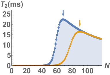
Figure 2: Plot of $T_{2}$ versus number of islands $N$. Fluxonium parameters are fixed at $E_{C}=2.5$, $E_{J}=9.0$, and $E_{L}=0.52$ GHz, as in experiment Manucharyan et al. (2009). These imply $e^{2}/2C^{b}=2.64$ GHz. Blue arrow indicates optimal choice $N=68$. The yellow curve shows a recalculation to check the effect of reduced wavefunction confinement, see Eq. 17, with the arrow indicating optimal choice $N=90$.

Fig. 2 considers the early fluxonium experiment Manucharyan et al. (2009). The blue curve indicates that, for the experimentally chosen parameters of $E_{C}$, $E_{J}$, $E_{L}$, and $C^{b}$, the optimal value of $N$ is $68$. The original device, with $N=43$, had a ratio of only $E_{J}^{a}/E_{C}^{a}\approx 22$, leading to excessive low-frequency charge noise dephasing. At the optimal $N$, $E_{J}^{a}/E_{C}^{a}\approx 53$, so the array junctions are deeper in the transmon regime, leading to better suppression of charge-noise dephasing.

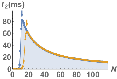
Figure 3: Plot of $T_{2}$ versus number of islands $N$. Fluxonium parameters are fixed at $E_{C}=0.55$, $E_{J}=2.2$, and $E_{L}=0.72$ GHz, as in device C of experiment Nguyen et al. . These imply $e^{2}/2C^{b}=0.73$ GHz. Blue arrow indicates optimal choice $N=12$. The yellow curve shows a recalculation to check the effect of reduced wavefunction confinement, see Eq. 17, with an arrow indicating optimal choice $N=18$. Similar results are obtained for the other devices in Nguyen et al. .

Fig. 3 provides an analogous plot for a recent experiment Nguyen et al. . The blue curve shows that the optimal choice is the relatively small value $N=12$, far less than the experimental value $N=102$. This striking reduction arises since the original device had array junctions with $E_{J}^{a}/E_{C}^{a}>3000$, far larger than needed to protect against low-frequency charge noise. The satisfactory value $E_{J}^{a}/E_{C}^{a}\approx 47$ is achieved at $N=12$; further increasing $N$ just brings about a faster relaxation rate $1/T_{1}$.

This kind of argument gives a general rule-of-thumb for the optimal $N$. Because the pure dephasing rate in LABEL:Eq:epsilon0 and 15 drops exponentially with $N$ while the relaxation rate in Eq. 16 increases only polynomially, the optimal number of junctions is just large enough to suppress the former. As shown in Fig. 4, this means that up to a logarithmic correction, $N_{\text{optimal}}\sim 5-10\times 1/\sqrt{E_{L}/{\cal E}_{C}^{a}}$. This value ensures that the array junctions are sufficiently “transmon-like” with $E_{J}^{a}/E_{C}^{a}\gtrsim 50$. The optimal fluxonium qubit incorporates the minimal number of junctions consistent with this constraint and the desired $E_{C}$, $E_{J}$, and $E_{L}$.

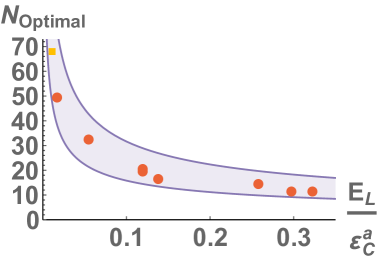
Figure 4: The optimal number of junctions $N$ as a function of the ratio $E_{L}/{\cal E}_{C}^{a}$. The square yellow data point on the left is taken from Manucharyan et al. (2009) while the remaining 8 data points are taken from Nguyen et al. . The region between the curves $5/\sqrt{E_{L}/{\cal E}_{C}^{a}}$ and $10/\sqrt{E_{L}/{\cal E}_{C}^{a}}$ is shaded, showing agreement with the rule-of-thumb for $N_{\text{optimal}}$.

Naturally, the millisecond-scale $T_{2}$ times in Figs. 2 and 3 exceed the much shorter values measured experimentally. This is unsurprising, because the figures only consider charge noise, neglecting all other mechanisms of decoherence. One expects that such mechanisms, like flux noise or Purcell emission, are functions of $E_{C}$, $E_{L}$, and $E_{J}$ that probably do not depend sensitively on $N$. It is plausible that some mechanisms could favor smaller fluxonium designs, in which case the optimal value $N=12$ found in Fig. 3 could only decrease.

Discussion —

The optimizations here should not require experimentally unrealistic parameters. We have fixed $C^{b}$, $E_{J}^{b}$ near their experimental values Manucharyan et al. (2009); Nguyen et al. while the values required for $C^{a}$ and $E_{J}^{a}$ should be attainable by scaling the area of the array junctions. For example, to realize the optimal point $N=12$ in Fig. 3, the array junctions should be modified to have an area about $12/102$ times what was chosen in the $N=102$ experiment. The resulting junctions would still be larger than the “black-sheep” junction (i.e., at the optimum $N$, $C^{a}>C^{b}$ and $E_{J}^{a}>E_{J}^{b}$). In any case, the superconducting qubit platform is characterized by remarkable experimental flexibility. There are many possibilities one could imagine to realize specified junction parameters, such as shunting each of the array junctions with its own transmon-style capacitor Koch et al. (2007).

One expects generally correct answers from the harmonic approximation (7) and the tight-binding approximation (LABEL:Eq:Psi0) that underlie our calculations. Symmetry considerations decidedly limit the effect of corrections to the harmonic approximation, as investigated thoroughly in Ferguson et al. (2013). In addition, as discussed above, the optimal $N$ depends only logarithmically on most of the parameters in the equation. However, some caution is appropriate – the harmonic approximation does exaggerate the confining potential, since $1-\cos\Theta_{i}\leq\Theta_{i}^{2}/2$. The Gaussian ground state wavefunctions $\phi_{0}$ are thus overly localized, suppressing the overlap between neighboring terms in LABEL:Eq:Psi0. As a result, the matrix element (LABEL:Eq:epsilon0) and dephasing rate (15) are somewhat underestimated.

To assess the amount of error that results, we consider the broadened Gaussian wavefunctions

$$\phi_{0}(\theta_{i})\to\sqrt{\lambda}\phi_{0}(\lambda\theta_{i}),$$ (17)

with $\lambda=2/\pi$. These would be the eigenstates of Eq. 7 if we changed $\Theta_{i}^{2}/2\to 2\Theta_{i}^{2}/\pi^{2}\leq 1-\cos\Theta_{i}$ to bound the Josephson potential from below. We use these revised $\phi_{0}$ to recalculate LABEL:Eq:epsilon0 . The result, shown as yellow curves in Figs. 2 and 3, is an increase of the optimum $N$ by around ${\pi/2-1\approx 50\%}$ and a modest decrease in the associated $T_{2}$. Of course, the yellow curves significantly overestimate the dephasing rate, and we expect the real value to be closer to the blue curves . It is also instructive to note that the transmon case, solved exactly using a Mathieu function Koch et al. (2007) without a tight-binding approximation, exhibits $\epsilon_{0}\sim e^{-\sqrt{8E_{L}/\mathcal{E}_{C}^{a}}}$, implying $\lambda\sim 8/\pi^{2}\approx 0.8$. This would increase our optimal values of $N$ in Figs. 2 and 3 by around $20\%$, intermediate between the blue and yellow curves. Taken together, these checks show that our approximations give the correct picture and only lead to modest quantitative errors.

The findings presented here identify an important potential optimization of the fluxonium design. Our prediction follows from the familiar charge-noise model described in Fig. 1b and is absent from earlier studies of fluxonium decoherence Manucharyan et al. (2012); Viola and Catelani (2015) that considered different forms of environmental noise. For instance, Manucharyan et al. (2012) instead assumed an admitttance in parallel with each of the Josephson junctions of the circuit, which naturally models dissipative current fluctuations (such as quasiparticle tunneling Catelani et al. (2011); Yan et al. (2016)) across the junctions. Thus, an experimental test of our results could shed light on the charge-noise model of superconducting qubits. Most importantly, a significant gain in device performance could result from our proposed optimization.

References

- Shnirman et al. (1997) A. Shnirman, G. Schön, and Z. Hermon, Phys. Rev. Lett. 79, 2371 (1997).
- Bouchiat et al. (1998) V. Bouchiat, D. Vion, P. Joyez, D. Esteve, and M. H. Devoret, Physica Scripta T76, 165 (1998).
- Nakamura et al. (1999) Y. Nakamura, Y. A. Pashkin, and J. S. Tsai, Nature 398, 786 (1999).
- Nakamura et al. (2002) Y. Nakamura, Y. A. Pashkin, T. Yamamoto, and J. S. Tsai, Phys. Rev. Lett. 88, 047901 (2002).
- Koch et al. (2007) J. Koch, T. M. Yu, J. Gambetta, A. A. Houck, D. I. Schuster, J. Majer, A. Blais, M. H. Devoret, S. M. Girvin, and R. J. Schoelkopf, Phys. Rev. A 76, 042319 (2007).
- Orlando et al. (1999) T. P. Orlando, J. E. Mooij, L. Tian, C. H. van der Wal, L. S. Levitov, S. Lloyd, and J. J. Mazo, Phys. Rev. B 60, 15398 (1999).
- Yan et al. (2016) F. Yan, S. Gustavsson, A. Kamal, J. Birenbaum, A. P. Sears, D. Hover, T. J. Gudmundsen, D. Rosenberg, G. Samach, S. Weber, J. L. Yoder, T. P. Orlando, J. Clarke, A. J. Kerman, and W. D. Oliver, Nature Communications 7, 12964 (2016).
- Manucharyan et al. (2009) V. E. Manucharyan, J. Koch, L. I. Glazman, and M. H. Devoret, Science 326, 113 (2009).
- Hazard et al. (2019) T. M. Hazard, A. Gyenis, A. Di Paolo, A. T. Asfaw, S. A. Lyon, A. Blais, and A. A. Houck, Phys. Rev. Lett. 122, 010504 (2019).
- Grünhaupt et al. (2019) L. Grünhaupt, M. Spiecker, D. Gusenkova, N. Maleeva, S. T. Skacel, I. Takmakov, F. Valenti, P. Winkel, H. Rotzinger, W. Wernsdorfer, A. V. Ustinov, and I. M. Pop, Nature Materials 18, 816 (2019).
- Niepce et al. (2019) D. Niepce, J. Burnett, and J. Bylander, Phys. Rev. Applied 11, 044014 (2019).
- Matveev et al. (2002) K. A. Matveev, A. I. Larkin, and L. I. Glazman, Phys. Rev. Lett. 89, 096802 (2002).
- Maleeva et al. (2018) N. Maleeva, L. Grünhaupt, T. Klein, F. Levy-Bertrand, O. Dupre, M. Calvo, F. Valenti, P. Winkel, F. Friedrich, W. Wernsdorfer, A. V. Ustinov, H. Rotzinger, A. Monfardini, M. V. Fistul, and I. M. Pop, Nature Communications 9, 3889 (2018).
- Manucharyan et al. (2012) V. E. Manucharyan, N. A. Masluk, A. Kamal, J. Koch, L. I. Glazman, and M. H. Devoret, Phys. Rev. B 85, 024521 (2012).
- Devoret (1997) M. H. Devoret, “Quantum fluctuations in electrical circuits,” in Quantum Fluctuations, edited by S. Reynaud, E. Giacobino, and J. Zinn-Justin (Elsevier, New York, 1997) Chap. 10, pp. 351–385.
- Caldeira and Leggett (1983) A. O. Caldeira and A. J. Leggett, Annals of Physics 149, 374 (1983).
- Ferguson et al. (2013) D. G. Ferguson, A. A. Houck, and J. Koch, Phys. Rev. X 3, 011003 (2013).
- Note (1) To carefully verify that satisfies the correct boundary conditions, regard the new variables as functions of the original variables . Add to any , and replace the index everywhere with ; returns to itself.
- Note (2) Note . This is unchanged, as to be expected, by a constant shift of all .
- (20) L. B. Nguyen, Y.-H. Lin, A. Somoroff, R. Mencia, N. Grabon, and V. E. Manucharyan, arXiv:1810.11006 .
- Zorin et al. (1996) A. B. Zorin, F.-J. Ahlers, J. Niemeyer, T. Weimann, H. Wolf, V. A. Krupenin, and S. V. Lotkhov, Phys. Rev. B 53, 13682 (1996).
- Krantz et al. (2019) P. Krantz, M. Kjaergaard, F. Yan, T. P. Orlando, S. Gustavsson, and W. D. Oliver, Applied Physics Reviews 6, 021318 (2019).
- Note (3) In each of the exponentials of LABEL:Eq:epsilon0, but not the prefactor, gets multiplied by . The term also gets multiplied by .
- Note (4) It is possible to treat as a variational parameter in LABEL:Eq:Psi0 and minimize the energy of to determine at each . The obtained is very close to 1 except at the smallest values of .
- Viola and Catelani (2015) G. Viola and G. Catelani, Phys. Rev. B 92, 224511 (2015).
- Catelani et al. (2011) G. Catelani, J. Koch, L. Frunzio, R. J. Schoelkopf, M. H. Devoret, and L. I. Glazman, Phys. Rev. Lett. 106, 077002 (2011).