Rho resonance, timelike pion form factor, and implications for lattice studies of the hadronic vacuum polarisation

Abstract

We study isospin-1 P-wave $\pi\pi$ scattering in lattice QCD with two flavours of O($a$) improved Wilson fermions. For pion masses ranging from $m_{\pi}=265$ MeV to $m_{\pi}=437$ MeV, we determine the energy spectrum in the centre-of-mass frame and in three moving frames. We obtain the scattering phase shifts using Lüscher’s finite-volume quantisation condition. Fitting the dependence of the phase shifts on the scattering momentum to a Breit-Wigner form allows us to determine the resonance parameters $m_{\rho}$ and $g_{\rho\pi\pi}$. By combining the scattering phase shifts with the decay matrix element of the vector current, we calculate the timelike pion form factor, $F_{\pi}$, and compare the results to the Gounaris-Sakurai representation of the form factor in terms of the resonance parameters. In addition, we fit our data for the form factor to the functional form suggested by the Omnès representation, which allows for the extraction of the charge radius of the pion. As a further application, we discuss the long-distance behaviour of the vector correlator, which is dominated by the two-pion channel. We reconstruct the long-distance part in two ways: one based on the finite-volume energies and matrix elements and the other based on $F_{\pi}$. It is shown that this part can be accurately constrained using the reconstructions, which has important consequences for lattice calculations of the hadronic vacuum polarisation contribution to the muon anomalous magnetic moment.

I Introduction

The study of hadronic resonances in terms of the underlying theory of QCD necessitates a non-perturbative treatment. Lattice QCD has emerged as a versatile tool enabling ab-initio determinations of many hadronic properties Aoki et al. (2019). The $\rho$ meson, which is the simplest QCD resonance and decays almost exclusively into two pions Tanabashi et al. (2018), is interesting for several reasons: It serves as a benchmark for the finite-volume formalism pioneered by Lüscher Lüscher (1986a, b); Rummukainen and Gottlieb (1995), whose practical implementation poses a number of challenging tasks. Furthermore, the relevant correlation function have a rather favourable noise-to-signal ratio compared to those for other resonances, due to the $\rho$ being the lightest isovector resonance.

Beyond its role as a benchmark, the precision study of the $\rho$ resonance has a number of interesting applications. A good understanding of the $\rho\rightarrow\pi\pi$ channel is a vital component for any study of more complicated resonances, where the $\rho$ is an intermediate decay channel. Thus, the $\rho$ has been subject to many lattice QCD studies already Aoki et al. (2007, 2011); Feng et al. (2011a); Lang et al. (2011); Pelissier and Alexandru (2013); Dudek et al. (2013a); Wilson et al. (2015); Bali et al. (2016); Bulava et al. (2016); Fu and Wang (2016); Andersen et al. (2019); Guo et al. (2016); Alexandrou et al. (2017); Werner et al. (2019). Secondly, using the approach suggested by Meyer Meyer (2011) (which is closely related to work by Lellouch and Lüscher Lellouch and Lüscher (2001)), the pion form factor, $F_{\pi}$, can be determined in lattice QCD in the timelike region. For first lattice implementations of this method see Feng et al. (2015a); Andersen et al. (2019).

An interesting and increasingly relevant application of lattice calculations of $F_{\pi}$ arises in the context of ab initio determinations of the hadronic vacuum polarisation (HVP) contribution to the muon’s anomalous magnetic moment, $a_{\mu}^{\rm hvp}$. The latter is accessible via the (spatially summed) vector correlator $G(x_{0})$ Bernecker and Meyer (2011); Francis et al. (2013); Feng et al. (2013), which, at large Euclidean times $x_{0}$ is dominated by the two-pion channel. Given sufficiently precise data for $F_{\pi}$, one can accurately constrain the long-distance regime of $G(x_{0})$ which helps to significantly reduce both statistical and systematic uncertainties in lattice calculations of $a_{\mu}^{\rm hvp}$ Meyer and Wittig (2019).

The outline of this paper is as follows: In Section II we summarise the methods used for determining the isospin-1 scattering phase shift and the timelike pion form factor from our lattice calculations. Section III presents our results for the scattering phase shift, while section IV contains the results for the timelike pion form factor. Implications for the calculation of the leading order HVP contribution to the muon anomalous magnetic moment $a_{\mu}$ are discussed in Section V. Finally, Section VI summarises our results. Our analysis supersedes previous preliminary results presented in Erben et al. (2016, 2018).

II Methodology

II.1 Determination of the finite volume energy spectrum

To study the $\rho$ resonance, we first need to extract a tower of low-lying energy levels. The strategy we use is to build a matrix of correlation functions using interpolating field operators with the quantum numbers of the $\rho$ meson. The lowest states of the spectrum can be extracted using the variational method Michael and Teasdale (1983); Michael (1985); Lüscher and Wolff (1990); Blossier et al. (2009). We start by forming a correlator matrix

$$C_{ij}(t)=\langle O_{i}(t)O_{j}(0)^{\dagger}\rangle=\sum_{n=1}^{\infty}e^{-E_{n}t}\langle 0|O_{i}|n\rangle\langle n|O_{j}^{\dagger}|0\rangle$$ (1)

from the correlators formed of interpolating operators $O_{i}(t)$ for the $\rho$ and $\pi\pi$ states in a given frame and then solve a generalised eigenvalue problem (GEVP)

$$C(t)\bm{v}(t,t_{0})=\lambda(t,t_{0})C(t_{0})\bm{v}(t,t_{0})$$ (2)

for this matrix. The $n^{th}$ eigenvalue $\lambda_{n}$ asymptotically decays exponentially with the energy $E_{n}$ of the $n^{th}$ state. There are different ways of choosing the parameter $t_{0}$ in the GEVP; one of them is to keep $t_{0}$ constant (the “fixed-$t_{0}$ method”) and another way is to use the “window method” Blossier et al. (2009), which keeps the window width $t_{w}=t-t_{0}$ constant. For suitable choices, the latter ensures that the leading excited state contamination to $\lambda_{n}(t,t_{0})$ from the finite correlator basis comes from $\Delta E_{n}=E_{N+1}-E_{n}$ Blossier et al. (2009), where $N$ is the size of the basis.

For the operator basis we use Feng et al. (2011b)

$$\rho^{0}(\bm{P},t) =\frac{1}{2L^{3/2}}\sum_{\bm{x}}e^{-i\bm{P}\cdot\bm{x}}\left(\bar{u}\Gamma u-\bar{d}\Gamma d\right)(t)\,,$$ (3)

where $\Gamma\in\{\gamma_{i},\gamma_{0}\gamma_{i}\}$ and

$$(\pi\pi)(\bm{p}_{1},\bm{p}_{2},t)=\pi^{+}(\bm{p}_{1},t)\pi^{-}(\bm{p}_{2},t)-\pi^{-}(\bm{p}_{1},t)\pi^{+}(\bm{p}_{2},t)\,.$$ (4)

The momenta $\bm{p}_{1}$ and $\bm{p}_{2}$ of the single pions add up to the frame momentum $\bm{P}$, i.e. $\bm{p}_{1}+\bm{p}_{2}=\bm{P}\equiv 2\pi/L\bm{d}$. The single-pion interpolators are defined by

$$\pi^{+}(\bm{q},t)= \frac{1}{2L^{3/2}}\sum_{\bm{x}}e^{-i\bm{q}\cdot\bm{x}}\big{(}\bar{u}\gamma_{5}d\big{)}(\bm{x},t)\,,$$ (5)

$$\pi^{-}(\bm{q},t)= \frac{1}{2L^{3/2}}\sum_{\bm{x}}e^{-i\bm{q}\cdot\bm{x}}\big{(}\bar{d}\gamma_{5}u\big{)}(\bm{x},t)\phantom{a}\,.$$ (6)

In a finite hypercubic volume, the rotational symmetry $O(3)$ of the continuum is reduced to that of a discrete subgroup. The operators are therefore classified by the irreducible representations (irreps) of the respective subgroup. The set of irreps depends on the momentum frame used. In this work, we are using a centre-of-mass frame (CMF) as well as moving frames with three different lattice momenta with a maximum momentum of $\bm{P}^{2}=3(2\pi/L)^{2}$, i.e. $\bm{d}^{2}=3$. Correlation functions are computed for all such moving frames that can be realised on a lattice of spatial size $L$. Frames that share the same absolute momentum are averaged over.

In the rest frame, continuum operators $O^{J}$ with spin $J$ are subduced Dudek et al. (2010) into the irreps $\Lambda$ of the octahedral group via

$$O^{[J]}_{\Lambda,\mu}=\sum_{M}\mathcal{S}_{\Lambda,\mu}^{J,M}O^{J,M}\,,$$ (7)

where $M$ are the magnetic quantum numbers of $J$, $\mathcal{S}_{\Lambda,\mu}^{J,M}$ are the subduction coefficients and $\mu$ is the row of the finite volume irrep $\Lambda$. The $J$ in $O^{[J]}_{\Lambda,\lambda}$ is in brackets because, although it was produced only from operators with spin $J$, the operator can now have an overlap with all other spins which are contained in $\Lambda$ Dudek et al. (2012).

In moving frames, there is a further reduction of symmetry, namely into the subgroup of the octahedral group that keeps $\bm{P}$ invariant Dudek et al. (2012), which is referred to as the little group Moore and Fleming (2006). To subduce continuum operators into the lattice irreps of the moving frame, we need helicity operators

$$O^{J,\lambda}(\bm{p})=\sum_{M}\mathcal{D}^{(J)*}_{M\lambda}(R)O^{J,M}(\bm{p})\,,$$ (8)

where $\lambda$ is the helicity index, and $\mathcal{D}^{(J)*}_{M\lambda}(R)$ is a Wigner-$\mathcal{D}$ matrix Wigner (1931) for the transformation $R$ that rotates $|\bm{p}|\hat{\bm{e}}_{z}$ into $\bm{p}$ Thomas et al. (2012). This allows a further subduction into little group irreps $\Lambda$, forming a so-called subduced helicity operator

$$O^{J,P,|\lambda|}_{\Lambda,\mu}(\bm{p})=\sum_{\hat{\lambda}=\pm\lambda}\mathcal{S}^{\tilde{\eta}\hat{\lambda}}_{\Lambda,\mu}O^{J,P,\hat{\lambda}}(\bm{p})\,,$$ (9)

where $P$ is the parity of $O^{J,P,\hat{\lambda}}(\bm{p}=0)$ and $\tilde{\eta}=P(-1)^{J}$.

We construct multiparticle operators from linear combinations of products of single-particle operators with definite momentum. A general $\pi\pi$ creation operator in an irrep $\Lambda$ can be written Dudek et al. (2012)

$$(\pi\pi)^{[\bm{p}_{1},\bm{p}_{2}]\dagger}_{\bm{P},\Lambda,\mu}=\sum_{\begin{subarray}{c}\bm{p}_{1}\in\{\bm{p}_{1}\}^{*}\\ \bm{p}_{2}\in\{\bm{p}_{2}\}^{*}\\ \bm{p}_{1}+\bm{p}_{2}=\bm{P}\end{subarray}}=\mathcal{C}(\bm{P},\Lambda,\mu,\bm{p}_{1},\bm{p}_{2})\pi^{\dagger}(\bm{p}_{1})\pi^{\dagger}(\bm{p}_{2})\,,$$ (10)

where $\{\bm{p}_{1,2}\}^{*}$ is the group orbit of $\bm{p}_{1,2}$, i.e. the set of momenta that are equivalent under an allowed lattice rotation. $\mathcal{C}$ is a Clebsch-Gordan coefficient which couples the irreps $\Lambda_{1}$ and $\Lambda_{2}$ of the single-pion creation operators $\pi^{\dagger}(\bm{p})$ with the irrep $\Lambda$ of the $(\pi\pi)^{\dagger}$ operator. These single-pion irreps are either the $A_{1}^{-}$ irrep of the cubic group for $\bm{p}=0$ or the $A_{2}$ irrep of the little group of $\bm{p}$ for $\bm{p}\neq 0$. The coefficients relevant for this work are listed in Dudek et al. (2012); Morningstar et al. (2013).

In the isospin limit G-parity allows only contributions from odd partial waves Dudek et al. (2013b). Taking these reductions of symmetry into account, the relevant irreps of the $\rho\rightarrow\pi\pi$ channel, where $J^{P}=1^{-}$ and where $l=1$ is the dominant contributing partial wave are listed in Table 1.

$\bm{d}$	$\Lambda(\bm{dim}(\Lambda))$
$[000]$	$T_{1}(3)$
$[00n]$	$A_{1}(1),E(2)$
$[0nn]$	$A_{1}(1),B_{1}(1),B_{2}(1)$
$[nnn]$	$A_{1}(1),E(2)$

Table 1: Irreps in the various moving frames used in this study.

In addition to the correlator matrix $C(t)$, the calculation of the timelike pion form factor in Section IV also requires the matrix elements $\langle J_{\mu}(\bm{x}=0,t)O_{i}^{\dagger}(0)\rangle$, both for the local (single-site) current,

$$J_{\mu}^{l}(x)=\frac{1}{2}Z_{V}\bar{\psi}(x)\gamma_{\mu}\tau^{3}\psi(x)\,,$$ (11)

and the conserved (point-split) current

$$J_{\mu}^{c}(x+\tfrac{a}{2}\hat{\mu})=\frac{1}{4}(\bar{\psi}(x+a\hat{\mu})(1+\gamma_{\mu})U_{\mu}(x)^{\dagger}\tau^{3}\psi(x)-\bar{\psi}(x)(1-\gamma_{\mu})U_{\mu}(x)\tau^{3}\psi(x+a\hat{\mu}))\,,$$ (12)

where $\psi(x)=(u,\,d)^{T}$ and $\tau^{3}={\mathrm{diag}}(1,\,-1)$. In analogy to the single-meson operators, the spatial components of the current operators $J_{\mu}(x)$ are projected into the respective irreps $\Lambda$, yielding $J^{\Lambda}(x)$. In what follows, the superscript $\Lambda$ will be omitted in all equations where the irreps are treated the same way.

We extract the relevant information on the ground state and the first few excited states from the eigenvectors $v_{n}(t)$ of the corresponding eigenvalues $\lambda_{n}(t)$ determined via the solution of the GEVP of $C(t)$.

The former are used to define operators $X_{n}(t)$ that project on the state with energy $E_{n}$:

$$X_{n}(t)=v_{n}^{\dagger}O(t)=\sum_{i}v_{ni}^{*}O_{i}\,.$$ (13)

The corresponding two-point function is defined as

$$D_{nn}(t)=\langle X_{n}(t)X^{\dagger}_{n}(0)\rangle=v_{n}^{\dagger}C(t)v_{n}\,,$$ (14)

which is the (approximate) projection of the correlation matrix $C_{ij}(t)$ onto the correlator corresponding to the $n^{th}$ state. We investigated the eigenvectors $v_{n}$ on each timeslice and have chosen to use the vectors from the earliest timeslice after which the absolute value of their components plateaued. At large times, remnant contributions from other states in $D_{nn}(t)$ are expected to be exponentially suppressed such that only the $n^{th}$ state survives:

$$D_{nn}(t)\rightarrow|Z_{n}|^{2}\exp(-E_{n}t)\,.$$ (15)

$Z_{n}=\langle\Omega|X_{n}|n\rangle$ is an overlap factor with state $n$ of the optimised interpolating operator $X_{n}$. From an exponential fit to $D_{nn}(t)$ we extract $|Z_{n}|$ for our further analysis. The operators $X_{n}$ are then used to form a two-point function with the current insertions at the sink,

$$\langle J(t)X_{n}^{\dagger}(0)\rangle=\sum_{i}v_{ni}\langle J(t)O_{i}^{\dagger}(0)\rangle\,,$$ (16)

which again has a large-time behaviour dominated just by one state:

$$\langle J(t)X_{n}^{\dagger}(0)\rangle\rightarrow\langle\Omega|J(t)|n\rangle Z_{n}^{*}e^{-E_{n}t}\,.$$ (17)

The timelike pion form factor requires the knowledge of the matrix element $\langle\Omega|J(t)|n\rangle$, which can either be extracted by fitting an exponential function to $D_{nn}(t)$ and $\langle J(t)X_{n}^{\dagger}(0)\rangle$ or by forming the ratio Andersen et al. (2019):

$$R^{E_{n}}(t) =\frac{\langle J(t)X_{n}^{\dagger}(0)\rangle}{\sqrt{D_{nn}(t)}e^{-\frac{1}{2}E_{n}t}}\rightarrow\frac{Z_{n}^{*}}{|Z_{n}|}\langle\Omega|J(t)|n\rangle\,.$$ (18)

We also computed two other ratios with the same asymptotic value proposed by the authors of Andersen et al. (2019). Similar to that work, we find $R(t)$ produces the most precise plateaus of the three and is not reliant on the fit to Equation (15) for the extraction of $Z_{n}$. Therefore we fit a constant to $|R^{E_{n}}(t)|^{2}=|\langle\Omega|J(t)|n\rangle|^{2}$ to extract the plateau value, which we denote $|A_{n}|^{2}$.

II.2 The distillation method

The two-pion operators are non-trivial to compute, due to so-called sink-to-sink quark lines which require all-to-all propagators to be computed. To facilitate this task we are using the “distillation” Peardon et al. (2009) and stochastic Laplacian Heavyside (LapH) smearing Morningstar et al. (2011) methods.

With distillation Peardon et al. (2009), a smearing matrix $\mathcal{S}_{xy}(t)$ is constructed in the following way: We start with the lattice spatial Laplacian,

$$-\nabla^{2}(\bm{x},\bm{y},t)=6\delta_{\bm{x},\bm{y}}-\sum_{j=1}^{3}(\tilde{U}_{j}(\bm{x},t)\delta_{\bm{x}+\hat{j},\bm{y}}+\tilde{U}_{j}^{\dagger}(\bm{y},t)\delta_{\bm{x}-\hat{j},\bm{y}})\,,$$ (19)

where the gauge fields $\tilde{U}$ have been smeared using $3$ iterations of stout smearing Morningstar and Peardon (2004) with smearing parameter $0.2$. We then compute the lowest $N_{\mathrm{ev}}$ eigenmodes $v^{(k)}$, defined via

$$\sum_{\bm{y}}-\nabla^{2}(\bm{x},\bm{y},t)v^{(k)}(\bm{y},t)=\lambda^{(k)}(t)v^{(k)}(\bm{x},t)\,.$$ (20)

The definition of the actual smearing matrix is

$$\mathcal{S}_{xy}(t)=\sum_{k=1}^{N_{\mathrm{ev}}}v^{(k)}(\bm{x},t)v^{\dagger(k)}(\bm{y},t)\equiv V(t)V^{\dagger}(t)\,.$$ (21)

One main advantage of this approach is that this smearing matrix can be split and used to project propagators into the subspace spanned by the $N_{\mathrm{ev}}$ eigenvectors, a much smaller number than the $3N_{L}^{3}$ colour fundamental fields on each timeslice which are naively needed to save a propagator.

Particularly on larger lattices, because the total computational cost scales with the cube of the physical volume or higher for fixed smearing, distillation is often treated stochastically Morningstar et al. (2011). In this approach noise-partitioning (also referred to as dilution) in the space spanned by the Laplacian eigenmodes Wilcox (1999); Foley et al. (2005) is used to reduce the variance of the stochastic estimator. With a suitable dilution scheme, using just one noise per quark line typically produces a statistical uncertainty due to the stochastic estimation of the quark propagation that is of the same size or smaller than the one from the Monte-Carlo path integral.

A quark line, i.e. a smeared-to-smeared propagator within stochastic Laplacian-Heavyside (LapH)-smearing, can be computed via

$$\mathcal{Q} =\mathcal{S}D^{-1}\mathcal{S}=\sum_{b}E(\varphi^{[b]}(\rho)(\varrho^{[b]}(\rho))^{\dagger})\,,$$ (22)

with the LapH sink vectors $\varphi$ and the LapH source vectors $\varrho$,

$$\varphi^{[b]}(\rho) =\mathcal{S}D^{-1}VP^{(b)}\rho$$ (23)

$$\varrho^{[b]}(\rho) =VP^{(b)}\rho\,.$$ (24)

These in turn are constructed using the noise vectors $\rho$, and the dilution projectors $P^{(b)}$. One can use $\gamma_{5}$-hermiticity to reverse quark propagators, giving rise to alternative LapH source and sink vectors

$$\bar{\varphi}^{[b]}(\rho) =\gamma_{5}\varphi^{[b]}(\rho)\,,$$ (25)

$$\bar{\varrho}^{[b]}(\rho) =\gamma_{5}\varrho^{[b]}(\rho)\,,$$ (26)

which give a different estimator for the quark line, $E(\bar{\varrho}\bar{\varphi}^{\dagger})$. Meson functions can then be expressed via

$$\mathcal{M}_{\Gamma}^{[b_{1},b_{2}],(\rho_{1},\rho_{2})}(\bm{v}_{1},\bm{w}_{2};\bm{p},t)=\Gamma_{\alpha\beta}\sum_{\bm{x}}e^{-i\bm{p}\cdot\bm{x}}\bm{v}^{[b_{1}]}_{a\alpha,\bm{x}t}(\rho_{1})^{*}\bm{w}^{[b_{2}]}_{a\beta,\bm{x}t}(\rho_{2})\,,$$ (27)

where $\bm{v},\bm{w}$ are LapH source or sink vectors $\varrho,\bar{\varrho}$ or $\varphi,\bar{\varphi}$. Single-meson correlation functions are a product of two such meson functions, for example

$$\langle\pi^{+}(t_{f})\pi^{-}(t_{0})\rangle =\frac{1}{4L^{3}}\langle-\mathcal{M}^{[b_{1},b_{2}],(\rho_{1},\rho_{2})}_{\gamma_{5}}(\bar{\varphi_{i}},\varphi_{j};t_{F})\mathcal{M}^{[b_{1},b_{2}],(\rho_{1},\rho_{2})}_{\gamma_{5}}(\bar{\varrho_{i}},\varrho_{j};t_{0})^{*}\rangle_{U,\rho}\,,$$ (28)

which uses the Einstein summation convention for the dilution indices $b_{1},b_{2}$. As our correlation functions can contain two-pion operators at both the source and the sink, we evaluate expressions with products of up to four meson functions.

Correlation functions with a vector current at the sink require a propagator that is not smeared at the sink. This can be computed via Mastropas and Richards (2014); Andersen et al. (2019)

$$D^{-1}\mathcal{S}=\sum_{b}E(\phi^{[b]}(\rho)(\varrho^{[b]}(\rho))^{\dagger}),$$ (29)

where $\phi$ is a LapH unsmeared sink vector,

$$\phi^{[b]}(\rho)=D^{-1}VP^{(b)}\rho,$$ (30)

and likewise $\bar{\phi}^{[b]}(\rho)=\gamma_{5}\phi^{[b]}(\rho)$ yields an estimator for $\mathcal{S}D^{-1}$.

II.3 Gauge field configurations and distillation schemes

We use three gauge field ensembles with 2 dynamical mass-degenerate light flavours of nonperturbatively improved Wilson quarks Sheikholeslami and Wohlert (1985); Jansen and Sommer (1998) generated by the Coordinated Lattice Simulations (CLS) consortium using the DDHMC algorithm and software package Lüscher (2005, 2007). The ensembles were generated with $\beta=5.3$ corresponding to a lattice spacing of $a=0.0658(7)(7)\mathrm{fm}$ and Table 2 lists key parameters of these ensembles along with the number of configurations used in our study.

	$T/a$	$L/a$	$m_{\pi}$ [MeV]	$\kappa$	$m_{\pi}L$	$N_{\mathrm{conf}}$	$N_{\mathrm{meas}}$	$N_{\mathrm{ev}}$
E5	64	32	437	0.13625	4.7	500	2000	56
F6	96	48	311	0.13635	5.0	300	900	192
F7	96	48	265	0.13638	4.2	350	1050	192

Table 2: CLS $N_{f}=2$ ensembles used in this study. All share $\beta=5.3$ and $a=0.0658(7)(7)\mathrm{fm}$. $T$ and $L$ refer to the lattice extent in time and space directions respectively. $N_{\mathrm{conf}}$ specifies the number of gauge configurations used, while $N_{\mathrm{meas}}$ refers to the number of source timeslices multiplied by the number of configurations. The number of Laplacian eigenmodes used is denoted by $N_{\mathrm{ev}}$.

We use different dilution schemes for quark lines connected to the source timeslice and for sink-to-sink quark lines. Lines connected to the source timeslice use full spin dilution and full time dilution. Full Laplacian eigenvector dilution is used on E5, while interlace-12 eigenvector dilution (LI12 in the notation of Morningstar et al. (2011)) is used on F6 and F7. The perambulators for sink-to-sink (sts) quark lines are calculated with full spin dilution and interlace-8 time dilution (TI8). On E5 sink-to-sink lines use LI8, while LI12 is used on F6 and F7.

For the calculation of Laplacian eigenmodes, the PRIMME package Stathopoulos and McCombs (2010) is used with a preconditioner built from Chebyshev polynomials Neff et al. (2001). Our code uses the library QDP++ from USQCD Edwards and Joó (2005) and the deflated SAP+GCR solver from the openQCD package Lüscher and Schaefer (2013). For cross-checks of the analysis the package TwoHadronsInBox Morningstar et al. (2017) was used.

III The $\rho$ resonance

In this section the determination of the energy spectra, the calculation of the phase shift from the energies, and the resulting resonance mass $m_{\rho}$ and coupling $g_{\rho\pi\pi}$ are described.

III.1 Energy spectra

The pion masses on the three ensembles have been extracted using a $\cosh$-fit ansatz. The fit ranges and results are shown in Table 3.

	$t_{\mathrm{min}}$	$t_{\mathrm{max}}$	$am_{\pi}$
E5	$15$	$28$	$0.14511(33)$
F6	$16$	$35$	$0.10366(29)$
F7	$19$	$40$	$0.08893(30)$

Table 3: Fit ranges to the single-cosh fit and corresponding pion masses including jackknife error on the three ensembles.

We also solved the GEVP in the window method for the 8 irreps listed in Table 1. The extracted energy levels of two selected irreps on the F6 lattice, together with the effective energies $E^{(k)}_{\mathrm{eff}}(t)=-t_{w}^{-1}\ln(\lambda^{(k)}(t))$ are shown in Fig. 1.

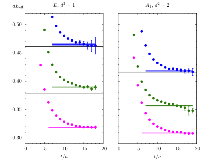
Figure 1: Spectrum from the GEVP on the F6 lattice, using the window method, for two irreps: $\bm{d}^{2}=1,E$ on the left (a typical example for the energy levels we extract) and $\bm{d}^{2}=2,A_{1}$ on the right (an example where the plateau does not look as good, particularly the intermediate level). The different levels in the respective irrep are plotted using different colours and the accordingly coloured bands are the fit results of the corresponding eigenvalues to fit function allowing for the ground state and an excited state. The width of those bands indicates the statistical error of the fit and the length shows the chosen fit range. The horizontal lines are the free two-pion levels in the respective moving frame.

The energy levels were obtained by fitting the eigenvalues extracted from the GEVP to a function allowing for the ground state and one excited state. Results for all irreps and ensembles are listed in Table 4, together with the values of $\chi^{2}$/d.o.f. for each fit.

$d^{2}$	irrep	E5	$\chi^{2}$/d.o.f.	F6	$\chi^{2}$/d.o.f.	F7	$\chi^{2}$/d.o.f.
		0.3213(11)	0.77	0.2883(9)	0.63	0.2727(11)	0.45
0	$T_{1}$	0.4905(21)	0.73	0.3443(15)	0.82	0.3306(17)	1.67
				0.4333(32)	0.42	0.4228(34)	0.75
		0.3022(8)	1.05	0.2329(10)	0.84	0.2049(8)	1.40
1	$A_{1}$	0.3573(12)	1.12	0.2996(15)	0.96	0.2875(18)	0.66
				0.3618(18)	1.24	0.3491(21)	1.04
		0.3215(14)	1.67	0.2900(10)	0.83	0.2755(11)	1.14
1	$E$	0.5238(41)	0.77	0.3671(18)	1.02	0.3559(18)	0.49
				0.4460(28)	0.35	0.4356(40)	0.56
		0.3068(11)	0.85	0.2472(10)	1.18	0.2224(11)	0.95
2	$A_{1}$	0.3783(20)	1.37	0.3054(17)	1.23	0.2945(21)	1.04
				0.3753(18)	0.61	0.3646(21)	1.77
		0.3155(25)	0.60	0.2658(10)	0.86	0.2467(11)	1.82
2	$B_{1}$	0.4128(20)	1.11	0.3106(18)	1.25	0.2948(29)	1.67
				0.3841(20)	1.48	0.3700(27)	0.43
		0.3240(23)	1.10	0.2913(13)	0.84	0.2783(17)	2.22
2	$B_{2}$	0.5454(51)	1.32	0.3755(18)	1.29	0.3653(20)	0.71
				0.3943(24)	1.06	0.3797(40)	0.78
		0.3096(18)	0.59	0.2584(13)	0.37	0.2364(17)	1.35
3	$A_{1}$	0.3937(47)	0.62	0.2989(14)	0.44	0.2831(20)	0.82
				0.3161(21)	0.97	0.3079(26)	0.82
3	$E$	0.3199(37)	1.83	0.2786(12)	1.41	0.2617(15)	0.73
		0.4538(37)	0.77	0.3295(18)	1.12	0.3132(34)	1.74

Table 4: Extracted energy levels $aE_{k}$ (states are ordered from ground state to the higher excited states from top to bottom) in the window method with $t_{w}$=3 in each irrep for the three lattices used in this work. One level fewer per irrep is extracted on E5, due to the levels being above the $4m_{\pi}$ threshold and the interpolator basis being smaller by 1.

III.2 Lüscher formalism

Lüscher’s finite volume method Lüscher (1986a, b) is used to map the energy levels of the finite-volume lattice box to the continuum phase shift. For the $\rho$, we are interested in the $l=1$ partial wave. In principle, higher partial waves also contribute to the spectrum. The effect of the $l=3$ and $l=5$ partial waves has been studied in Dudek et al. (2013a); Andersen et al. (2019). With this restriction, the quantisation condition reads

$$\delta_{1}(k)=\phi^{\bm{d}}_{\Lambda}(q)+n\pi\,.$$ (31)

In this equation, $k=(2\pi/L)q$ are the scattering momenta, $\delta_{1}(k)$ is the $l=1$ infinite volume phase shift, and $\phi^{\bm{d}}_{\Lambda}(q)$ is a kinematical function related to modified zeta functions, which can be computed to arbitrary precision. The centre-of-mass energy is given by $E_{\textrm{cm}}=2\sqrt{m_{\pi}^{2}+k^{2}}$. With the spectrum data from the GEVP we can use this relation to map out the infinite volume phase shift in the energy region $2m_{\pi}<E<4m_{\pi}$.

The results from this procedure are shown in Fig. 2 for all three ensembles used.

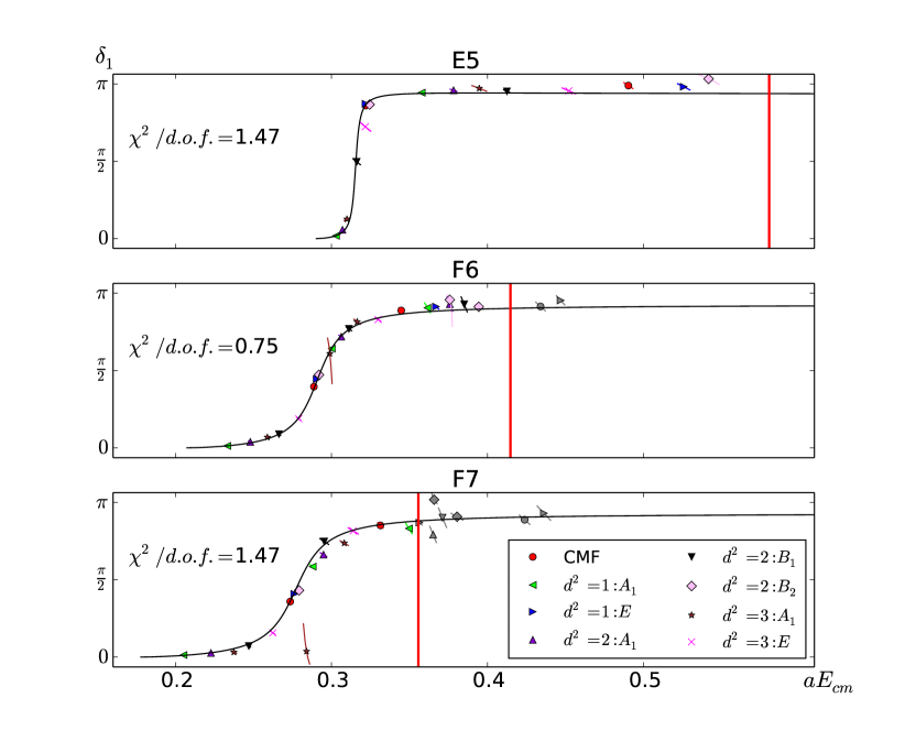
Figure 2: Phase shifts on all three ensembles using the window method. The horizontal axis shows the CMF energy of each level and data points of the same colour and symbol belong to the same frame and irrep. Error bars follow the curves allowed by the Lüscher zeta functions. The red vertical line indicates the $4m_{\pi}$ threshold in each system; data points above are excluded from the fit and thus shown in grey. The black line is the result of the Breit-Wigner fit to our data by minimising the $\chi^{2}$ functional defined in (35). The $\chi^{2}$/d.o.f. for each fit is shown in the plots.

The curve in this plot is a fit to a Breit-Wigner parameterisation,

$$k^{3}\cot\delta_{1}^{\mathrm{BW}}(k;g_{\rho\pi\pi},m_{\rho}) =\frac{6\pi}{g_{\rho\pi\pi}^{2}}(m_{\rho}^{2}-E_{\textrm{cm}}^{2})E_{\textrm{cm}}\,,$$ (32)

which is motivated in the resonance region by the effective-range formula. Given that the data points and their error estimates are confined to the curves dictated by the Lüscher zeta function, as is visible in Fig. 2, we fit the data according to their error behaviour along the curves dictated by the zeta-functions. The Lüscher condition is reformulated to

$$\cot\delta_{1}(k)=\cot(\phi(q))\,,$$ (33)

and the difference to Equation (32),

$$f(q;g_{\rho\pi\pi},m_{\rho})=\cot(\phi(q))-\cot\delta_{1}^{\mathrm{BW}}\bigg{(}\frac{2\pi}{L}q;g_{\rho\pi\pi},m_{\rho}\bigg{)}\,,$$ (34)

is calculated. Given any pair of resonance parameters $(g_{\rho\pi\pi},m_{\rho})$ we can solve $f(q;g_{\rho\pi\pi},m_{\rho})=0$, and this way obtain $q_{i}^{\textrm{fit}}(g_{\rho\pi\pi},m_{\rho})$ and the energy levels $E_{\textrm{cm},i}^{\textrm{fit}}(g_{\rho\pi\pi},m_{\rho})$. To this end define the $\chi^{2}$-function

$$\chi^{2}(g_{\rho\pi\pi},m_{\rho}) =\sum_{i,j}(E_{\textrm{cm},i}^{\textrm{fit}}(g_{\rho\pi\pi},m_{\rho})-E_{\textrm{lat},i})C^{-1}_{i,j}(E_{\textrm{cm},j}^{\textrm{fit}}(g_{\rho\pi\pi},m_{\rho})-E_{\textrm{lat},j})\,,$$ (35)

with the covariance matrix

$$C_{i,j} =\sum_{k=0}^{n_{\textrm{jk}}}(E_{\textrm{lat},i,k}-\bar{E}_{\textrm{lat},i})(E_{\textrm{lat},j,k}-\bar{E}_{\textrm{lat},j})\,,$$ (36)

calculated from the $n_{\textrm{jk}}$ jackknife samples of the lattice energies and their central values $\bar{E}_{\textrm{lat},i}$. By minimising this $\chi^{2}$-function on each jackknife sample, we can obtain fit values for the resonance parameters. One advantage of this approach is that we can use any parameterisation suitable for the situation. We can compare our form factor results to the Gounaris-Sakurai parameterisation Gounaris and Sakurai (1968) of the phase shift, which is characterised by the resonance parameters $m_{\rho}$ and $\Gamma_{\rho}=\frac{k_{\rho}^{3}}{m_{\rho}^{2}}\frac{g_{\rho\pi\pi}^{2}}{6\pi}$:

$$\frac{k^{3}}{E_{\mathrm{cm}}}\cot[\delta_{1}^{\mathrm{GS}}(k)]=k^{2}h(E_{\mathrm{cm}})-k^{2}_{\rho}h(m_{\rho})+(k^{2}-k_{\rho}^{2})b\,,$$ (37)

$$b=-\frac{2}{m_{\rho}}\bigg{[}\frac{2k_{\rho}^{3}}{m_{\rho}\Gamma_{\rho}}+\frac{1}{2}m_{\rho}h(m_{\rho})+k_{\rho}^{2}h^{\prime}(m_{\rho})\bigg{]}\,,$$ (38)

$$h(\omega)=\frac{2k_{\omega}}{\pi\omega}\ln\frac{\omega+2k_{\omega}}{2m_{\pi}}\,,$$ (39)

$$k_{\omega}=\sqrt{\frac{\omega^{2}}{4}-m_{\pi}^{2}}\,,\quad k_{\rho}=k_{m_{\rho}}\,,$$ (40)

and show the results in Table 5. The two fits produce consistent results, although the Gounaris-Sakurai parameterisation yields slightly higher values of $\chi^{2}$.

	E5		F6		F7
	BW	GS	BW	GS	BW	GS
$m_{\rho}$	0.3156(8)	0.3157(10)	0.2933(8)	0.2934(9)	0.2800(10)	0.2800(10)
$g_{\rho\pi\pi}$	5.70(9)	5.66(9)	6.08(13)	6.03(13)	5.91(17)	5.88(16)
$\chi^{2}$/d.o.f.	1.47	1.64	0.75	0.84	1.47	1.52

Table 5: Resonance parameters extracted from the fit to the energy levels using the Lüscher formalism. All levels are extracted using the window method with $t_{w}$=3. Compared are the fit results to the Breit-Wigner and Gounaris-Sakurai parameterisations.

Figure 3 shows the world data for the coupling $g_{\rho\pi\pi}$ from various 2 and 2+1 flavor simulations. There is no significant dependence on the pion mass, and the lattice results are generally close to the physical value.

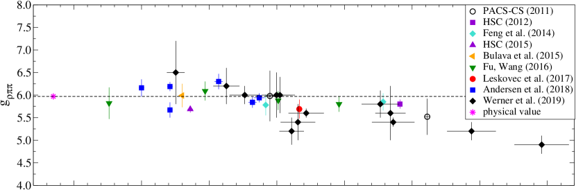
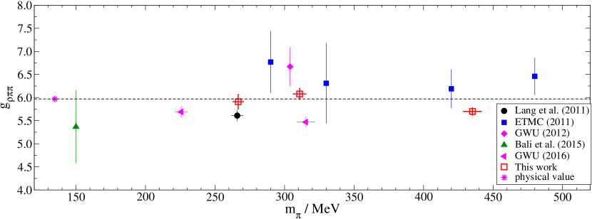
Figure 3: Overview of lattice results for the coupling $g_{\rho\pi\pi}$ as a function of the pion mass in the calculation. The upper pane shows the results from simulations with dynamical light and strange quarks, while the lower pane shows results with dynamical light quarks only. Where available, the scale-setting uncertainty provided by the authors has been added in quadrature to obtain the errors on the horizontal axis. The value extracted from the physical $\rho$-meson width is indicated by the magenta star and the black dashed line. The results from this work are the red open squares in the lower pane.

$d^{2}$	irrep	E5		F6		F7
$Z_{V}$		$0.74418(33)$		$0.74143(14)$		$0.74011(23)$
		$|A_{l}|$	$|A_{c}|$	$|A_{l}|$	$|A_{c}|$	$|A_{l}|$	$|A_{c}|$
		2.41(34)	2.12(31)	1.94(22)	1.74(19)	1.79(24)	1.63(22)
0	$T_{1}$	0.75(20)	0.57(16)	1.06(18)	0.90(16)	1.05(17)	0.90(15)
				0.71(22)	0.53(18)	0.80(20)	0.65(18)
		2.02(25)	1.81(22)	0.55(7)	0.51(6)	0.48(6)	0.46(5)
1	$A_{1}$	1.85(25)	1.59(22)	2.18(30)	1.95(26)	2.08(30)	1.87(26)
				0.79(14)	0.66(12)	0.87(15)	0.74(13)
		2.24(33)	1.98(30)	1.94(21)	1.74(19)	1.79(23)	1.63(21)
1	$E$	1.18(35)	0.97(30)	0.89(16)	0.74(14)	0.98(16)	0.82(14)
				0.57(17)	0.42(14)	0.52(14)	0.40(11)
		2.44(32)	2.17(28)	0.83(10)	0.77(9)	0.72(10)	0.68(9)
2	$A_{1}$	1.57(26)	1.33(23)	2.25(32)	2.00(28)	2.22(33)	1.98(29)
				0.65(12)	0.54(10)	0.63(11)	0.53(10)
		2.05(39)	1.81(35)	1.02(12)	0.93(11)	0.82(11)	0.76(11)
2	$B_{1}$	0.98(17)	0.81(15)	1.77(25)	1.56(22)	1.76(30)	1.57(26)
				0.43(10)	0.33(9)	0.50(10)	0.41(9)
		2.18(41)	1.92(37)	1.91(24)	1.71(21)	1.77(27)	1.60(24)
2	$B_{2}$	0.61(19)	0.50(16)	0.38(8)	0.31(7)	0.16(4)	0.14(4)
				0.92(18)	0.74(15)	0.87(20)	0.69(16)
		2.75(44)	2.44(40)	1.17(15)	1.08(13)	1.01(17)	0.94(16)
3	$A_{1}$	1.41(31)	1.17(26)	1.27(18)	1.12(15)	0.98(14)	0.87(13)
				1.87(29)	1.63(26)	2.05(33)	1.81(29)
3	$E$	1.42(33)	1.25(30)	1.40(18)	1.26(15)	1.25(18)	1.14(17)
		0.78(17)	0.64(14)	1.40(22)	1.20(19)	1.40(25)	1.21(22)

Table 6: Matrix elements $|A_{l/c}|$ extracted from the window method in units of $10^{-2}$. The values for $Z_{V}$ are taken from Della Morte et al. (2017). The difference in $|A_{l}|$ and $|A_{c}|$ is likely due to cut-off effects, which are studied in Della Morte et al. (2017); Gérardin et al. (2019).

IV The timelike pion form factor

To determine the timelike pion form factor we first need to calculate the matrix elements $|A_{l/c}|_{n}=|\langle 0|J_{l/c}|n\rangle|$. The subscripts $l/c$ refer to the local and the conserved currents, respectively. Our results for the matrix elements $|A_{l/c}|$ are listed in Table 6. There are sizable differences between $|A_{l}|$ and $|A_{c}|$, likely due to cut-off effects, which are studied in Della Morte et al. (2017); Gérardin et al. (2019). This is a clear indication that an improved version of the currents (defined e.g. in Lüscher et al. (1996, 1997)) would be preferable. These differences are supposed to vanish in the continuum limit, but we cannot check this since we are only considering a single lattice spacing.

We now have all the input to compute the timelike pion form factor Meyer (2011); Feng et al. (2015b),

$$|(F_{\pi})^{\bm{d}}_{\Lambda}(s)|^{2}=G^{\bm{d}}_{\Lambda}(\gamma)\Big{(}q(\phi^{\bm{d}}_{\Lambda})^{\prime}(q)+k\frac{\partial\delta_{1}(k)}{\partial k}\Big{)}\frac{3\pi s}{k^{5}}|A|^{2}\,,$$ (41)

where $s=E_{\mathrm{cm}}^{2}$ and

$$G^{\bm{d}}_{\Lambda}(\gamma)=\begin{cases}\frac{1}{\gamma}\phantom{aa}\mathrm{if}\phantom{aa}\Lambda=A_{1}\\ \gamma\phantom{aa}\mathrm{otherwise}\end{cases}\,,$$ (42)

with the Lorentz-boost $\gamma=\frac{E}{E_{\mathrm{cm}}}$.

This equation includes derivatives of the infinite volume phase shift $\delta_{1}(k)$ obtained in the previous section, and of the modified Lüscher zeta functions $\phi^{\bm{d}}_{\Lambda}$, which were also used in the phase-shift analysis, and which can be obtained to any desired mathematical precision. We want to compare our form factor results to another study Della Morte et al. (2017), which was performed on the same ensembles and which used correlators with one local and one conserved vector current. To conform with that study, we define the local-conserved version of $|A|^{2}$,

$$|A_{lc}|^{2}\equiv|A_{l}||A_{c}|\,.$$ (43)

For another literature comparison Brandt et al. (2013), we use the local-local version.

Equation (41) allows us to directly determine $F_{\pi}(s)$ from lattice data for discrete values of $s$, using a parameterisation of the phase shift as well as the current matrix elements. To get a continuous description of $F_{\pi}(s)$, we can use the Gounaris-Sakurai parameterisation Gounaris and Sakurai (1968), given by the resonance parameters $m_{\rho},\Gamma_{\rho}$:

$$F_{\pi}^{\mathrm{GS}}(E_{\mathrm{cm}}) =\frac{f_{0}}{\frac{k^{3}}{E_{\mathrm{cm}}}(\cot[\delta_{1}^{\mathrm{GS}}(k)]-i)}\,,$$ (44)

$$f_{0} =-\frac{m_{\pi}^{2}}{\pi}-k_{\rho}^{2}h(m_{\rho})-b\frac{m_{\rho}^{2}}{4}\,,$$ (45)

with the definitions from Eqs. (37 – 40). The comparison of our lattice-calculated values for $F_{\pi}$ and the Gounaris-Sakurai curves is shown in Figure 4. We want to stress these these curves are not fits to the form factor data.

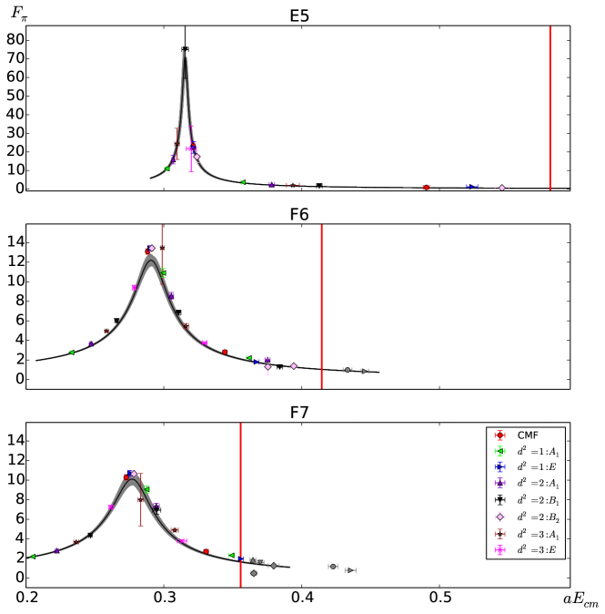
Figure 4: The timelike pion form factor on the E5, F6, F7 ensembles (top to bottom). Data points with the same symbol and colour belong to the same frame and irreps. The error bars associated with each data point come from a jackknife estimate. The grey curve is the GS representation of $F_{\pi}$, which only takes the fit parameters of the phase-shift fit $m_{\rho},g_{\rho\pi\pi}$ into account — it is not a fit to the data pictured in these plots. The vertical red bars indicate the $4m_{\pi}$ threshold for each lattice.

The Gounaris-Sakurai curve seems to describe our data reasonably well, but it would be desirable to have a fit to our form factor data extracted from lattice QCD. One way to realise such a fit is an $n$-subtracted Omnès representation Guo et al. (2009a); Guerrero (1998)

$$F_{\pi}^{(n)}(s)=\exp\Bigg{(}P_{n-1}(s)s+\frac{s^{n}}{\pi}\int_{4m_{\pi}^{2}}^{\infty}ds^{\prime}\frac{\delta_{1}(s^{\prime})}{(s^{\prime})^{n}(s^{\prime}-s-i\epsilon)}\Bigg{)}\,,$$ (46)

where $P_{n-1}(s)$ is a polynomial function of degree $n-1$. We parametrise the phase shift $\delta_{1}(s^{\prime})$ in this equation using the Breit-Wigner form, Equation (32), and our extracted resonance parameters. For the $2$-subtracted version, the polynomial is a constant,

$$P_{1}(s)=\frac{\langle r_{\pi}^{2}\rangle}{6}\,,$$ (47)

with the square radius $\langle r_{\pi}^{2}\rangle$ of the pion. The polynomial for the $3$-subtracted version reads

$$P_{2}(s)=\frac{\langle r_{\pi}^{2}\rangle}{6}+\frac{1}{2}\Big{(}2c_{V}^{\pi}-\Big{(}\frac{\langle r_{\pi}^{2}\rangle}{6}\Big{)}^{2}\Big{)}s\,,$$ (48)

with the curvature $c_{V}^{\pi}$ of the pion form factor. The integrand of

$$O_{n}(s)=\exp\Bigg{(}\frac{s^{n}}{\pi}\int_{4m_{\pi}^{2}}^{\infty}ds^{\prime}\frac{\delta_{1}(s^{\prime})}{(s^{\prime})^{n}(s^{\prime}-s-i\epsilon)}\Bigg{)}$$ (49)

has a pole at $s^{\prime}=s$ and in order to solve the integral numerically we need to do a subtraction,

$$\int_{4m_{\pi}^{2}}^{\infty}ds^{\prime}\frac{\delta_{1}(s^{\prime})}{(s^{\prime})^{n}(s^{\prime}-s-i\epsilon)}=\int_{4m_{\pi}^{2}}^{\infty}ds^{\prime}\frac{\delta_{1}(s^{\prime})-\delta_{1}(s)}{(s^{\prime})^{n}(s^{\prime}-s)}+\delta_{1}(s)\int_{4m_{\pi}^{2}}^{\infty}ds^{\prime}\frac{1}{(s^{\prime})^{n}(s^{\prime}-s-i\epsilon)}\,.$$ (50)

The integral $O(s)$ can now be computed analytically. We divide the lattice data $F_{\pi}(s)$ by the function $O_{n}(s)$, and fit the result using the function $f_{\mathrm{fit}}(s)=\exp(P_{n-1}(s)s)$. The results of the fit to the $3$-subtracted version are shown in Figure 5. In the $2$-subtracted version, our data were not very well described by the fit function. The fit describes the $F_{\pi}$ data much better than the GS representation of the form factor, but for all ensembles the fits have somewhat large values for $\chi^{2}/\mathrm{d.o.f.}$ We investigated the cause of this and excluded autocorrelation in the chain or single outlying data points as sources for this observation. There are however indications that our data set might be too small for reliable estimates of such a large covariance matrix.

Results for the square radius $\langle r_{\pi}^{2}\rangle$ from this fit are shown in Table 7. The results for the $2$- and $3$-subtracted version differ on the level of $2\sigma$, which is another indication that the $2$-subtracted version is not enough to describe the data accurately. The square radius was previously determined in Brandt et al. (2013) by fitting the spacelike pion form factor, computed on the same ensembles we are using in our study. This is a completely different approach and provides a very good cross-check of our fit procedure. Because the authors of Brandt et al. (2013) employ a local current (as opposed to the local-conserved setup used up to this point), we repeated the analysis using $|A_{l}|$ in Equation (41). The results for the square radius from this analysis are shown and compared to the result from Brandt et al. (2013) in Table 8. While both results agree very well for ensembles E5 and F6, we obtain a somewhat smaller square radius on ensemble F7. This observation is discussed further in Section V. The comparison of this table with Table 7 shows again that discretisation effects in our currents are sizable.

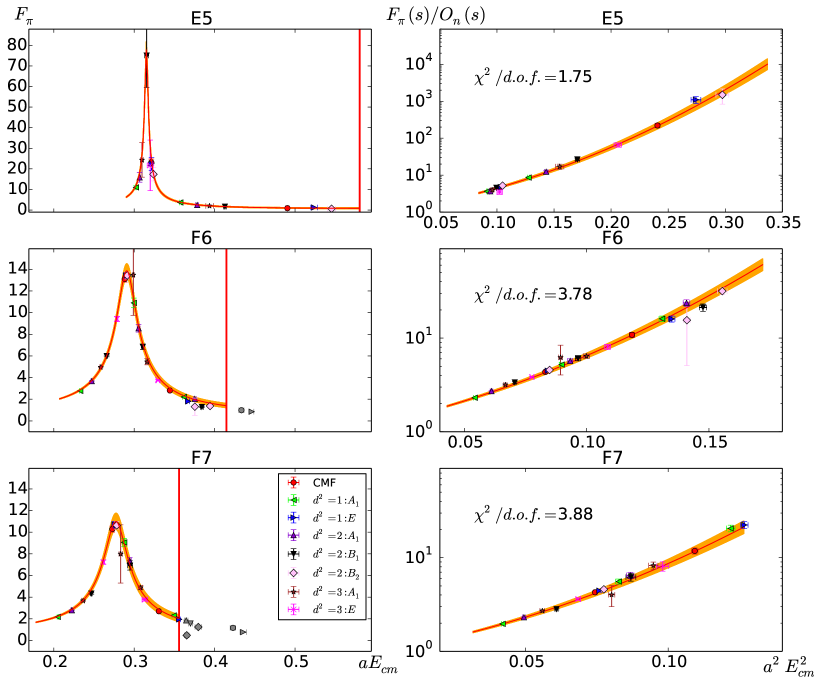
Figure 5: Left panel: The timelike pion form factor on the E5, F6, F7 lattice (top to bottom), window method. Data points with the same symbol and colour belong to the same frame and irreps. The orange curve is the fit to $F_{\pi}$, parametrised via the $3$-subtracted version of Equation (46). The vertical red bars indicate the $4m_{\pi}$ threshold in each lattice and data points above this threshold have not been included in the fit and are shown in grey for this reason. Right panel: The data which we are actually fitting to. The vertical axis shows $F_{\pi}$ divided by the Omnès integral, i.e. the analytically calculable part of Equation (46), and the fit function is $f(s)=\exp(Ps)$, where P is a 1st-order polynomial. The vertical axis is displayed on a $\log$ scale and the orange curve is the fit function with the jackknife error. Shown are also the $\chi^{2}/\mathrm{d.o.f.}$ values of the respective fits, which are quite high.

	$n$	E5	F6	F7
$\langle r_{\pi}^{2}\rangle/r_{0}^{2}$	2	1.18(2)	1.34(1)	1.46(2)
$\langle r_{\pi}^{2}\rangle/r_{0}^{2}$	3	1.11(3)	1.31(3)	1.37(4)
$c_{V}/r_{0}^{4}$	3	3.59(7)	4.98(7)	6.05(15)

Table 7: Square radius and curvature (in units of $10^{-2}$) of the pion obtained from the fit to the $n$-subtracted Omnès representation of the form factor, using a local-conserved current setup. The Sommer scale $r_{0}$ is taken from Fritzsch et al. (2012). We want to stress that the curvature can indeed be calculated from the fit parameter we use, but that the result and particularly the error estimate presented here might not be the physical value.

	$n$	E5	F6	F7
$\langle r_{\pi}^{2}\rangle/r_{0}^{2}$	2	1.25(2)	1.41(1)	1.53(2)
$\langle r_{\pi}^{2}\rangle/r_{0}^{2}$	3	1.18(3)	1.37(3)	1.43(4)
$c_{V}/r_{0}^{4}$	3	3.81(7)	5.26(8)	6.33(15)
$\langle r_{\pi}^{2}\rangle/r_{0}^{2}$ Brandt et al. (2013)		1.18(5)	1.37(6)	1.61(10)

Table 8: Same as Table 7 but using a local-local vector current. The last line shows the values from Brandt et al. (2013), where $\langle r_{\pi}^{2}\rangle$ has been computed from a fit to the spacelike form factor. The difference of our results to the corresponding values in Table 7 comes from discretisation effects, which are also visible in the matrix elements themselves, shown in Table 6.

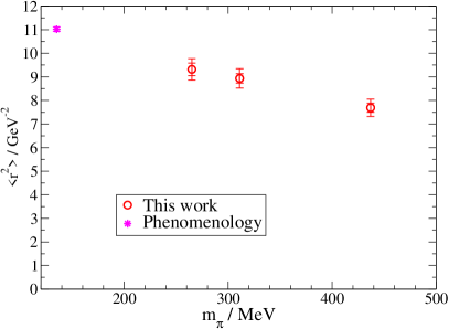
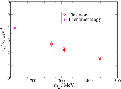
Figure 6: Left panel: Pion mass dependence of the square radius $\langle r_{\pi}^{2}\rangle$. Right panel: The same for the curvature $c_{v}$. Our lattice results are compared to the determinations in Ref. Colangelo et al. (2019) and Ref. Gonzàlez-Solís and Roig (2019) respectively. The inner error bar on the lattice data denotes the statistical uncertainty, while the outer error bar includes the scale setting uncertainty from the conversion to physical units.

As a consistency check our results for the square radius and curvature are plotted as a function of the pion mass, along with the values from phenomenological determinations in Figure 6. For the square radius we compare to the recent determination from Ref. Colangelo et al. (2019), while for the curvature we use the value from Ref. Gonzàlez-Solís and Roig (2019), which also provides an overview of various determinations. Note that the pion mass dependence of our results is in good qualitative agreements with the expectations from Ref. Guo et al. (2009b). Lattice results for the curvature have previously been obtained in Aoki et al. (2009).

V Hadronic vacuum polarisation

Recently, it has been realised that the timelike pion form factor has an important application in the context of lattice calculations of the hadronic contributions to the muon $g-2$. The hadronic vacuum polarisation contribution, $a_{\mu}^{\rm hvp}$, is accessible in lattice QCD via several integral representations involving the vector correlator Meyer and Wittig (2019). A convenient way to evaluate $a_{\mu}^{\rm hvp}$ is based on the so-called time-momentum representation (TMR) Bernecker and Meyer (2011); Francis et al. (2013); Feng et al. (2013):

$$a_{\mu}^{\mathrm{hvp}}=\Big{(}\frac{\alpha}{\pi}\Big{)}^{2}\int_{0}^{\infty}dx_{0}\,G(x_{0})\tilde{K}(x_{0};m_{\mu})\,,$$ (51)

with a known kernel function $\tilde{K}(x_{0};m_{\mu})$, the muon mass $m_{\mu}$ and the vector-vector correlator,

$$G(x_{0})\delta_{kl}=-\int d^{3}x\,\langle J^{\mathrm{em}}_{k}(x)J^{\mathrm{em}}_{l}(0)\rangle\,.$$ (52)

Here, $J^{\mathrm{em}}_{\mu}$ is the electromagnetic current,

$$J^{\mathrm{em}}_{\mu}(x)=\frac{2}{3}\bar{u}(x)\gamma_{\mu}u(x)-\frac{1}{3}\bar{d}(x)\gamma_{\mu}d(x)-\frac{1}{3}\bar{s}(x)\gamma_{\mu}s(x)+\cdots\,.$$ (53)

A definition of the kernel can be found in Della Morte et al. (2017). This correlator can be decomposed into an iso-vector ($I=1$) and an iso-scalar ($I=0$) part, $G(x_{0})=G^{I=1}(x_{0})+G^{I=0}(x_{0})$. It is also commonly decomposed into connected diagrams from each quark flavour and disconnected diagrams. For comparison with Ref. Della Morte et al. (2017), we will focus on the connected light-quark contribution, $G^{ud}(x_{0})=\frac{10}{9}G^{I=1}(x_{0})$. While for small $x_{0}$, this correlator can be precisely computed on the lattice, the signal cannot be traced to arbitrarily large values of $x_{0}$, partly due to the deteriorating signal-to-noise ratio, but also due to the finite time extent of the lattice. Getting a good estimate for the long-distance behaviour of $G(x_{0})$, which is needed to perform the integral to infinity, is one of the main challenges. The general idea is therefore to use the direct lattice data up to some cut-off distance $x_{0}^{\mathrm{cut}}$ and to determine the part above this distance separately. Ref. Della Morte et al. (2017) used a simplistic single-exponential model for the large-time part of $G^{ud}(x_{0})$:

$$G^{ud}(x_{0})=ce^{-m_{\rho}x_{0}}\,,$$ (54)

where $m_{\rho}$ was a naive estimate for the rho mass, namely the plateau value of a $\langle\rho(t)\rho^{\dagger}(0)\rangle$ correlator, and $c$ was determined by fitting $G^{ud}(x_{0})$. We are improving on this method in our work using two different approaches, one using a reconstruction of the finite-volume correlator and one estimating the infinite-volume correlator.

The finite-volume approach uses the information we have about the lowest states in the energy spectrum from the GEVP. We can reconstruct the light-quark correlator with the current matrix elements $|A_{l/c}|$ we already used to compute $F_{\pi}$,

$$G^{ud}_{n_{\mathrm{max}}}(x_{0})=\frac{10}{9}\sum_{n=0}^{n_{\mathrm{max}}}|A_{lc}|^{2}_{n}e^{-E_{n}x_{0}}\,.$$ (55)

This approach has several advantages: Not only do we get a more precise estimate for the large-$x_{0}$ behaviour of $G^{ud}(x_{0})$, but we also have a way to determine the number of states required for a reliable estimate. By computing $G^{ud}_{n_{\mathrm{max}}}(x_{0})$ for different values of $n_{\mathrm{max}}$, we can see the estimates converging towards each other. In a region where $G^{ud}_{n}(x_{0})$ agrees within errors with $G^{ud}_{n+1}(x_{0})$, we assume that all energy levels $n+2$ and above will not contribute significantly to $G^{ud}(x_{0})$. The integrand of Equation (51) for different values of $n_{\mathrm{max}}$ can be seen in Figure 7. We compare it to the data obtained by a direct calculation of the vector-vector correlator on the same ensembles, performed in Della Morte et al. (2017). Even for values lower than $x_{0}^{\mathrm{cut}}$, the contribution obtained only from the first level on E5 saturates the contribution from the lowest two levels. On F6 and F7, the contribution from two levels saturates the contribution obtained from 3 levels, also at comparably low $x_{0}$. This means that the computation of further levels would not contribute significantly to $a_{\mu}^{\mathrm{hvp}}$, and it also shows that a 1-exponential tail is not well motivated on F6 and F7. Also, on E5 and F6, our reconstructed data saturate the lattice data from Della Morte et al. (2017) around $x_{0}^{\mathrm{cut}}$ and are much more precise afterwards. On F7, the correlator data lie significantly above the reconstruction, which might be caused by a correlated fluctuation upward that overestimates the vector-vector correlator. Already starting at about $1$ fm, the data from the direct lattice calculation on F7 seem to deviate from the expected behaviour, leading to this possible overestimation.

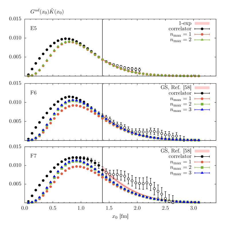
Figure 7: The light quark contribution to the integrand of Equation (51) for ensembles E5, F6, F7 (top to bottom). The data points computed in Della Morte et al. (2017) are plotted as black filled circles up to $x_{0}^{\mathrm{cut}}$ and as open circles above the cut. The bands represent the continuation of the correlator above $x_{0}^{\mathrm{cut}}$ as discussed in Ref. Della Morte et al. (2017). Coloured symbols denote the data from this work using the reconstructed light-quark correlator $G^{ud}_{n_{\mathrm{max}}}$ from Equation (55) for different values of $n_{\mathrm{max}}$. The vertical lines indicate the value of $x_{0}^{\mathrm{cut}}$.

In the infinite-volume approach, the long-time part of the correlator is estimated by evaluating the integral

$$G^{ud}_{F_{\pi}}(x_{0})=\frac{10}{9}\int_{0}^{\infty}d\omega\,\omega^{2}\rho(\omega^{2})e^{-\omega x_{0}}\,.$$ (56)

Below the $4m_{\pi}$ threshold, $\rho(s)$ can be parameterised by

$$\rho(s)=\frac{1}{48\pi^{2}}\bigg{(}1-\frac{4m_{\pi}^{2}}{s}\bigg{)}^{\frac{3}{2}}|F_{\pi}(s)|^{2}\,.$$ (57)

This approach was also used in Della Morte et al. (2017), where the form factor was estimated using the Gounaris-Sakurai Gounaris and Sakurai (1968) parameterisation using the naive rho mass $m_{\rho}$ and an estimation of the width $\Gamma_{\rho}$ based on its experimental value and an assumed scaling $\Gamma_{\rho}\propto k_{\rho}^{3}/m_{\rho}^{2}$.

In this work, we have several parameterisations of $F_{\pi}$ and can therefore directly evaluate Equation 56. The result of this is shown in Figure 8, where we compare the vector-vector correlator $G^{ud}_{F_{\pi}}$ obtained from the Gounaris-Sakurai and from the Omnès representation and for comparison show the estimator with the highest $n_{\text{max}}$ from Figure 7 as well as the Mainz HVP data from Della Morte et al. (2017) again. It is obvious that the Gounaris-Sakurai representation with the resonance parameters from our phase-shift analysis is not a good parameterisation of our data and leads to an integrand that does not saturate the lattice data.

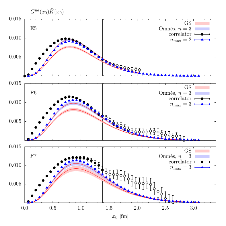
Figure 8: The integrand of Equation (51) for ensembles E5, F6, F7 (top to bottom). The meaning of the black filled and open circles is the same as in Figure 7. Blue triangles represent the integrand reconstructed from the iso-vector correlator $G^{ud}_{n_{\mathrm{max}}}$ of Equation (55) for the corresponding value of $n_{\mathrm{max}}$. Data corresponding to the iso-vector correlator constructed from the GS parameterisation and the $3$-subtracted Omnès representation of $F_{\pi}$ are shown as red and blue bands, respectively. The different types of extending the correlator above $x_{0}^{\mathrm{cut}}$ are used to compute the results for $a_{\mu}^{\mathrm{hvp}}$ presented in Table 9. The difference between the $2$- and $3$-subtracted versions of the Omnès representation integral is too small to be seen on this plot.

	E5	F6	F7
$0$ to $x_{0}^{\mathrm{cut}}$	2.662(26)	3.131(52)	3.462(86)
$x_{0}^{\mathrm{cut}}$ to $\infty$ (1-exp/GS)	0.484(15)	0.818(52)	1.238(96)
$x_{0}^{\mathrm{cut}}$ to $\infty$ ($G^{ud}_{n_{\mathrm{max}}}$)	0.473(9)	0.808(13)	1.050(20)
$x_{0}^{\mathrm{cut}}$ to $\infty$ ($G^{ud}_{F_{\pi}},n=2$)	0.516(13)	0.776(29)	1.049(48)
$x_{0}^{\mathrm{cut}}$ to $\infty$ ($G^{ud}_{F_{\pi}},n=3$)	0.502(13)	0.805(30)	1.078(52)
$0$ to $\infty$ (1-exp/GS)	3.146(39)	3.949(99)	4.700(173)
$0$ to $\infty$ ($G^{ud}_{n_{\mathrm{max}}}$)	3.135(28)	3.940(59)	4.524(95)
$0$ to $\infty$ ($G^{ud}_{F_{\pi}},n=2$)	3.179(30)	3.907(63)	4.511(102)
$0$ to $\infty$ ($G^{ud}_{F_{\pi}},n=3$)	3.165(31)	3.936(65)	4.540(106)
FV correction, $n=2$	0.043(12)	$-0.032(31)$	$-0.001(50)$
FV correction, $n=3$	0.029(13)	$-0.003(31)$	$0.028(54)$
FV correction, Della Morte et al. (2017)		0.03	0.07

Table 9: Values for $a_{\mu}^{\mathrm{hvp}}$ obtained using various methods, in units of $10^{-8}$. The first line shows the accumulated integral over the lattice data up to $x_{0}^{\mathrm{cut}}$. The next four lines show the integral over the long-time tail using the following four methods: (1-exp/GS) is the single-exponential (on E5) or the finite-volume GS parametrisation (on F6 and F7), which is a re-analysis of the data from Della Morte et al. (2017). $G^{ud}_{n_{\mathrm{max}}}$ is our extension using the reconstruction of the light-quark correlator using Equation (55). $G^{ud}_{F_{\pi}}$ reconstructs the vector-vector correlator using Equation (56), where the pion form factor $F_{\pi}$ is parametrised by the $n$-subtracted Omnès representation for $n=2$ and $n=3$. We do not show the results of $G^{ud}_{F_{\pi}}$ reconstructed using the GS parameterisation of $F_{\pi}$ as it does not describe our data well, as can be seen in Figure 8. The last three lines show the estimate of a correction for finite-volume effects, based on the difference between $G^{ud}_{F_{\pi}}$ and $G^{ud}_{n_{\mathrm{max}}}$, or based on the GS parametrisations in Ref. Della Morte et al. (2017) (which was not done for E5).

Table 9 shows our results for the long-time tail computed using the different methods employed in this work and compares them to the naive estimate obtained in Della Morte et al. (2017) without access to the resonance data from this work. Also shown is the full value for $a_{\mu}^{\mathrm{hvp}}$, which is the sum of the contribution from the direct lattice calculation and the different long-time tails. One can see readily from Figure 7 that on F7, our reconstruction of the vector-vector correlator using Equation (55) does not saturate the data from the direct lattice computation of $G^{ud}(x_{0})$. When comparing our new values for $a_{\mu}^{\mathrm{hvp}}$ with the ones from Della Morte et al. (2017) and the chiral extrapolation performed in that work (see Figure 9), one can see that the value for F7 shifts significantly, but that it comes to an overall better agreement with the chiral extrapolation curve. Because the lattice data on F7 seems to show a large correlated fluctuation already at about $1$ fm, and because we are using a transition value of $x_{0}^{\mathrm{cut}}\approx 1.38$ fm, the true value for $a_{\mu}^{\mathrm{hvp}}$ might be even lower. In any case, the published value for F7 lay prominently above the fit curve of the data points sharing the same lattice spacing and our analysis brought this data point closer to the curve. A similar issue is observed for the pion radius when comparing our results in Table 8 to the published results in Brandt et al. (2013).

Although asymptotically finite-volume effects in $G^{ud}(x_{0})$ are suppressed exponentially as $e^{-m_{\pi}L}$, in practice these effects can be significant. When the large-$x_{0}$ region is dominated by a small number of states, the volume dependence is not in the asymptotic regime Bernecker and Meyer (2011). Therefore, it is useful to consider the difference between infinite-volume and finite-volume reconstructions, which provides an estimate of a finite-volume correction. This is also shown in Table 9. On ensemble E5, the correction is statistically significant and roughly $+1\%$. On F6 and F7, where a finite-volume correction was previously estimated in Ref. Della Morte et al. (2017), our results are consistent with zero and also consistent with the previous estimate.

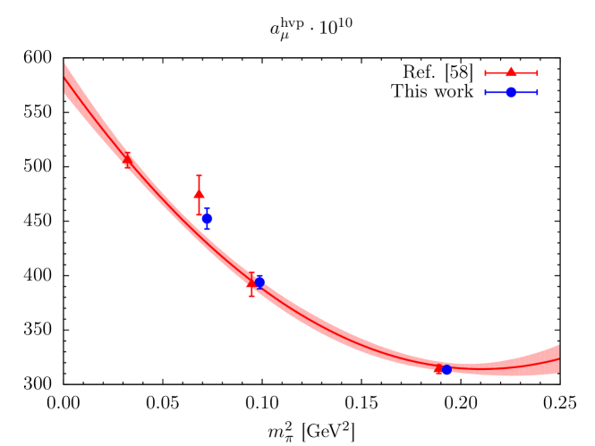
Figure 9: Pion mass dependence of $a_{\mu}^{\mathrm{hvp}}$ at $\beta=5.3$. Red triangle correspond to the data computed in Ref. Della Morte et al. (2017) with the chiral extrapolation at non-zero lattice spacing represented by the band. The blue circles denote the data points determined from the large-$x_{0}$ tail of our most precise reconstruction of the correlator, which is the $G^{ud}_{n_{\mathrm{max}}}$ correlator using the matrix elements $|A|$ as an input. Points are slightly shifted for clarity. The leftmost red triangle corresponds to ensemble G8 ($m_{\pi}=185$ MeV), which was not considered in this work. Our determination of the tail of the iso-vector correlator allows for a significantly more precise determination of $a_{\mu}^{\mathrm{hvp}}$ compared to Ref. Della Morte et al. (2017). Furthermore, we find that the result for F7 moves closer to the curve when our reconstruction of the large-distance tail is used.

VI Conclusions

We have performed an analysis of $I=1$ pion-pion scattering on three different $N_{f}=2$ ensembles at fixed lattice spacing. Our spectra have been determined using the variational method for a total of eight different irreps in the centre-of-mass frame and three different moving frames with lattice momenta up to $\bm{d}^{2}=3$. The spectral information was used in a finite-volume analysis to determine the resonance parameters. We have studied the consistency of different parameterisations of the phase shift by comparing the results for the resonance mass $m_{\rho}$ and the coupling $g_{\rho\pi\pi}$ obtained from fits to either the Breit-Wigner or the Gounaris-Sakurai representation. Our results, shown in Table 5, indicate that the resonance parameters are only weakly dependent on the parametrisation.

We have used our parameterisation of the phase-shift together with the matrix elements of the local and point-split vector currents to compute the pion form factor, $F_{\pi}$, in the timelike region. While the results for $F_{\pi}$ agree qualitatively with the Gounaris-Sakurai parameterisation based on our $\rho$ meson masses and couplings, they are better described by an Omnès representation obtained from a fit to the $F_{\pi}$ data, taking the resonance parameters $m_{\rho}$ and $g_{\rho\pi\pi}$ as input quantities.

The thrice-subtracted version provides a particularly good description and also allows for the determination of the (squared) pion charge radius $\langle r_{\pi}^{2}\rangle$. Our results compare well to an independent calculation of the charge radius on the same ensembles, obtained from the slope of the pion form factor in terms of the spacelike momentum transfer $Q^{2}$ Brandt et al. (2013). When lowering the pion mass, our results for $\langle r_{\pi}^{2}\rangle$ and the curvature approach the phenomenological values Colangelo et al. (2019); Gonzàlez-Solís and Roig (2019). The resulting mass dependence of the squared radius is compatible with the results in Ref. Guo et al. (2009b).

While the characterisation of resonances using lattice techniques is interesting in its own right, the gained information can also be put to good use in different contexts. As another important application we have considered the calculation of the hadronic vacuum polarisation contribution to the muon anomalous magnetic moment, $a_{\mu}^{\mathrm{hvp}}$. The precision of lattice calculations of $a_{\mu}^{\mathrm{hvp}}$ is typically limited by the long-distance tail of the vector correlator.

By means of a direct comparison with an earlier study Della Morte et al. (2017), we have shown that the precision in $a_{\mu}^{\mathrm{hvp}}$ can be substantially increased by describing the long-distance tail of the TMR integrand (see Equation (51)) using the spectral information on the first few states in the iso-vector channel. Alternatively, the tail of the integrand can be much more accurately constrained via the representation of the vector correlator in terms of the pion form factor. These techniques have, in the meantime, been employed in a recent calculation of $a_{\mu}^{\mathrm{hvp}}$ on CLS gauge ensembles with $N_{f}=2+1$ flavours of dynamical quarks Gérardin et al. (2019). Going beyond that work, we have used the difference between infinite-volume and finite-volume reconstructions to estimate finite-volume effects; the results are consistent with previous estimates using the Gounaris-Sakurai model.