Generic predictions of output probability based on complexities of inputs and outputs

Abstract

For a broad class of input-output maps, arguments based on the coding theorem from algorithmic information theory (AIT) predict that simple (low Kolmogorov complexity) outputs are exponentially more likely to occur upon uniform random sampling of inputs than complex outputs are. Here, we derive probability bounds that are based on the complexities of the inputs as well as the outputs, rather than just on the complexities of the outputs. The more that outputs deviate from the coding theorem bound, the lower the complexity of their inputs. Our new bounds are tested for an RNA sequence to structure map, a finite state transducer and a perceptron. These results open avenues for AIT to be more widely used in physics.

Deep links between physics and theories of computation Mezard and Montanari (2009); Moore and Mertens (2011) are being increasingly exploited to uncover new fundamental physics and to provide novel insights into theories of computation. For example, advances in understanding quantum entanglement are often expressed in sophisticated information theoretic language, while providing new results in computational complexity theory such as polynomial time algorithms for integer factorization Shor (1994). These connections are typically expressed in terms of Shannon information, with its natural analogy with thermodynamic entropy.

There is, however, another branch of information theory, called algorithmic information theory (AIT) Li and Vitanyi (2008), which is concerned with the information content of individual objects. It has been much less applied in physics (although notable exceptions occur, see Devine (2014) for a recent overview). Reasons for this relative lack of attention include that AIT’s central concept, the Kolmogorov complexity $K_{U}(x)$ of a string $x$, defined as the length of the shortest program that generates $x$ on a universal Turing machine (UTM) $U$, is formally uncomputable due to its link to the famous halting problem of UTMs Turing (1936). Moreover, many important results, such as the invariance theorem which states that for two UTMs $U$ and $W$, the Kolmogorov complexities $K_{U}(x)=K_{W}(x)+\mathcal{O}(1)$ are equivalent, hold asymptotically up to $\mathcal{O}(1)$ terms that are independent of $x$, but not always well understood, and therefore hard to control.

Another reason applications of AIT to many practical problems have been hindered can be understood in terms of hierarchies of computing power. For example, one of the oldest such categorisations, the Chomsky hierarchy Chomsky (1956), ranks automata into four different classes, of which the UTMs are the most powerful, and finite state machines (FSMs) are the least. Many key results in AIT are derived by exploiting the power of UTMs. Interestingly, if physical processes can be mapped onto UTMs, then certain properties can be shown to be uncomputable Lloyd (1993); Cubitt et al. (2015). However, many problems in physics are fully computable, and therefore lower on the Chomsky hierarchy than UTMs. For example, finite Markov processes are equivalent to FSMs, and RNA secondary structure (SS) folding algorithms can be recast as context-free grammars, the second level in the hiearchy. Thus, an important cluster of questions for applications of AIT revolve around extending its methods to processes lower in computational power than UTMs.

To explore ways of moving beyond these limitations and towards practical applications, we consider here one of the most iconic results of AIT, namely the coding theorem of Solomonoff and Levin Solomonoff (1964); Levin (1974), which predicts that upon randomly chosen programs, the probability $P_{U}(x)$ that a universal Turing machine (UTM) generates output $x$ can be bounded as $2^{-K(x)}\leq P(x)\leq 2^{-K(x)+{\mathcal{O}}(1)}$. Given this profound prediction of a general exponential bias towards simplicity (low Kolmogorov complexity) one might have expected widespread study and applications in science and engineering. This has not been the case because the theorem unfortunately suffers from the general issues of AIT described above (see however Delahaye and Zenil (2012); Zenil et al. (2014); Soler-Toscano et al. (2014) for important attempts to apply the full coding theorem).

Nevertheless, it has recently been shown Dingle et al. (2018); Zenil et al. (2019) that a related exponential bias towards low complexity outputs obtains for a range of non-universal input-output maps $f:I\rightarrow O$ that are lower on the Chomsky hierarchy than UTMs.

Figure 1: The probability $P(x)$ that a particular output arises upon random sampling of inputs versus output complexity $\tilde{K}(x)$ shows clear simplicity bias for: (a) A length $L=15$ RNA sequence to SS mapping, (b) An FST, sampled over all $2^{30}$ binary inputs of length $30$, and (c) A 7-input perceptron with weights discretised to 3 bits. The black solid line is the simplicity bias bound (1) (with $a$ and $b$ fit). For all these maps high complexity outputs occur with low probability. The outputs are colour coded by the maximum complexity $K_{\text{\rm max}}(p|n)$ of the set of inputs mapping to output $x$. Outputs further from the bound have lower input complexities. Figs (d) length $L=15$ RNA, (e) the FST and (d) the perceptron, show the data plotted for the lower bound (8) (black line) with only the intercept fit to the data, the slope is a prediction. The orange line is using Eq (8) with a normalised probability for a parameter free predictor. Including the complexity of the input through $K_{\text{\rm max}}(p|n)$ reduces the spread in the data, and so provides more predictive power than $K(x)$ alone.

In particular, an upper bound on the probability $P(x)$ that an output obtains upon uniform random sampling of inputs,

$$P(x)\leq 2^{-a\tilde{K}(x)-b}\,$$ (1)

was recently derived Dingle et al. (2018) using a computable approximation $\tilde{K}(x)$ to the Kolmogorov complexity of $x$, typically calculated using lossless compression techniques. Here $a$ and $b$ are constants that are independent of $x$ and which can often be determined from some basic information about the map. The so-called simplicity bias bound (1) holds for computable maps $f$ where the number of inputs $N_{I}$ is much greater than the number of outputs $N_{O}$ and the map $K(f)$ is simple, meaning that asymptotically $K(f)+K(n)\ll K(x)+\mathcal{O}(1)$ for a typical output $x$, where $n$ specifies the size of $N_{I}$, e.g. $N_{I}=2^{n}$. Eq. (1) typically works better for larger $N_{I}$ and $N_{O}$. Approximating the true Kolmogorov complexity also means that the bound shouldn’t work for maps where a significant fraction of outputs have complexities that are not qualitatively captured by compression based approximations. For example many pseudo random-number generators are designed to produce outputs that appear to be complex when measured by compression or other types of Kolmogorov complexity approximations. Yet these outputs must have low $K(x)$ because they are generated by relatively simple algorithms with short descriptions. Nevertheless, it has been shown that the bound (1) works remarkably well for a wide class of input-output maps, ranging from the sequence to RNA secondary structure map, to systems of coupled ordinary differential equations, to a stochastic financial trading model, to the parameter-function map for several classes of deep neural networks Dingle et al. (2018); Pérez et al. (2018); Mingard et al. (2019).

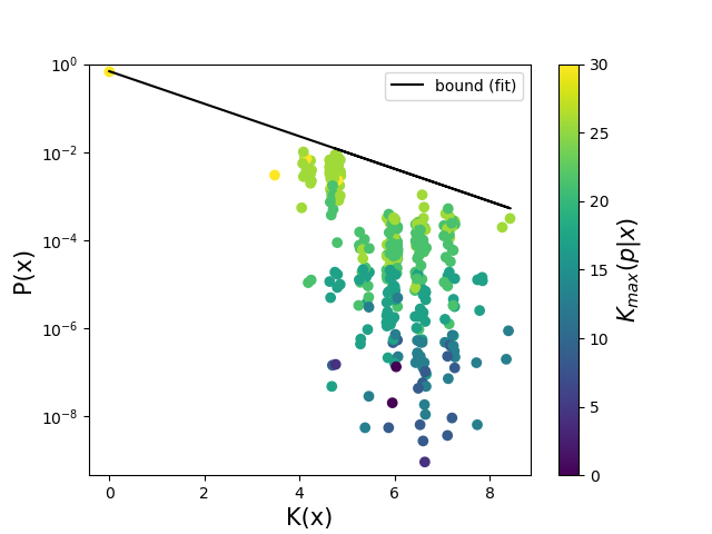
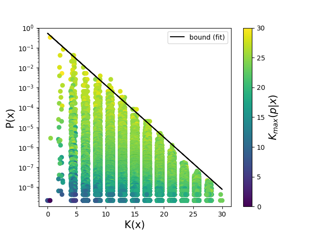
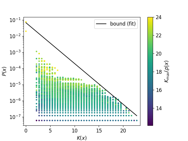
The simplicity bias bound (1) predicts that high $P(x)$ outputs will be simple, and that complex outputs will have a low $P(x)$. But, in sharp contrast to the full AIT coding theorem, it doesn’t have a lower bound, allowing low $\tilde{K}(x)$ outputs with low $P(x)$ that are far from the bound. Indeed, this behaviour is generically observed for many (non-universal) maps Dingle et al. (2018); Pérez et al. (2018) (see also Fig 1), but should not be the case for UTMs that obey the full coding theorem. Understanding the behaviour of outputs far from the bound should shed light on fundamental differences between UTMs and maps with less computational power that are lower on the Chomsky hierarchy, and may open up avenues for wider applications of AIT in physics.

With this challenge in mind, we take an approach that contrasts with the traditional coding theorem of AIT or with the simplicity bias bound, which only consider the complexity of the outputs. Instead, we derive bounds that also take into account the complexity of the inputs that generate a particular output $x$. While this approach is not possible for UTMs, since the halting problem means one cannot enumerate all inputs Li and Vitanyi (2008), and so averages over input complexity cannot be calculated, it can be achieved for non-UTM maps. Among our main results, we show that the further outputs are from the simplicity bias bound (1), the lower the complexity of the set of inputs. Since, by simple counting arguments, most strings are complex Li and Vitanyi (2008), the cumulative probability of outputs far from the bound is therefore limited. We also show that by combining the complexities of the output with that of the inputs, we can obtain better bounds on and estimates of $P(x)$.

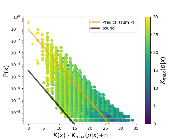
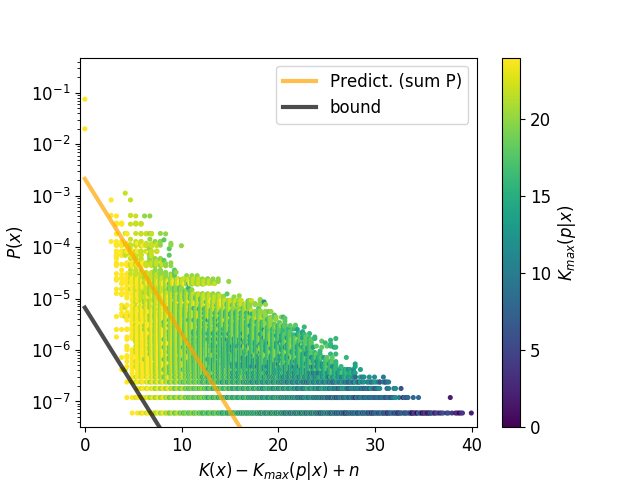
Whether such bounds nevertheless have real predictive power needs to be tested empirically. Because input based bounds typically need exhaustive sampling, full testing is only possible for smaller systems, which restricts us here to maps where finite size effects may still play a role Dingle et al. (2018). We test our bounds on three systems, the famous RNA sequence to secondary structure map (which falls into the context-free class in the Chomsky hierarchy), here for a relatively small size with length $L=15$ sequences, a finite state transducer (FST), a very simple input-output map that is lowest on the Chomsky hierarchy Chomsky (1956), with length $L=30$ binary inputs, and finally the parameter-function map Valle-Pérez et al. (2018); Mingard et al. (2019) of a perceptron Rosenblatt (1958) with discretized weights to allow complexities of inputs to be calculated. The preceptron plays a key role in deep learning neural network architectures  LeCun et al. (2015). Nevertheless, as can be seen in Fig. 1(a-c) all three maps exhibit simplicity bias predicted by Eq (1), even if they are relatively small. In Ref. Dingle et al. (2018), much cleaner simplicity bias behaviour can be observed for larger RNA maps, but these are too big to exhaustively sample inputs. Similarly, cleaner simplicity bias behaviour occurs for the undiscretised perceptron Mingard et al. (2019), but then it is hard to analyse the complexity of the inputs.

Fig. 1(a-c) shows that the complexity of the input strings that generate each output $x$ decreases for further distances from the simplicity bias bound. This is the kind of phenomenon that the we will attempt to explain.

To study input based bounds, consider a map $f:I\rightarrow O$ between $N_{I}$ inputs and $N_{O}$ outputs that satisfies the requirements for simplicity bias Dingle et al. (2018). Let $f(p)=x$, where $p$ is some input program $p\in I$ producing output $x\in O$. For simplicity let $p\in\{0,1\}^{n}$, so that all inputs have length $n$ and $N_{I}=2^{n}$ (this restriction can be relaxed later). Define $f^{-1}(x)$ to be the set of all the inputs that map to $x$, so that the probability that $x$ obtains upon sampling inputs uniformly at random is

$$P(x)=\frac{|f^{-1}(x)|}{2^{n}}\,$$ (2)

Any arbitrary input $p$ can be described using the following $\mathcal{O}(1)$ procedure Dingle et al. (2018): Assuming $f$ and $n$ are given, first enumerate all $2^{n}$ inputs and map them to outputs using $f$. The index of a specific input $p$ within the set $f^{-1}(x)$ can be described using at most $\log_{2}(|f^{-1}(x)|)$ bits. In other words, this procedure identifies each input by first finding the output $x$ it maps to, and then finding its label within the set $f^{-1}(x)$. Given $f$ and $n$, an output $x=f(p)$ can be described using $K(x|f,n)+\mathcal{O}(1)$ bits Dingle et al. (2018). Thus, the Kolmogorov complexity of $p$, given $f$ and $n$ can be bounded as:

$$K(p|f,n)\leq K(x|f,n)+\log_{2}(|f^{-1}(x)|)+\mathcal{O}(1).$$ (3)

We note that this bound holds in principle for all $p$, but that it is tightest for $K_{\rm max}(p|x)\equiv\max_{p}\{K(p|f,n)\}$ for $p\in f^{-1}(x)$. More generally, we can expect these bounds to be fairly tight for the maximum complexity $K_{\text{\rm max}}(p|f,n)$ of inputs due to the following argument. First note that

$$K_{\text{\rm max}}(p|f,n)\geq\log_{2}(|f^{-1}(x)|)+{\mathcal{O}}(1)$$ (4)

because any set of $|f^{-1}(x)|$ different elements must have strings of at least this complexity. Next,

$$K(x|f,n)\leq K(p|f,n)+{\mathcal{O}}(1)$$ (5)

because each $p$ can be used to generate $x$. Therefore:

$$\max(K(x|f,n),\log_{2}(|f^{-1}(x)|))\leq K_{\text{\rm max}}(p|f,n)+{\mathcal{O}}(1),$$ (6)

so the bound (3) cannot be too weak. In the worst case scenario, where $K_{\text{\rm max}}(p|n)\approx\log_{2}(|f^{-1}(x)|)\approx K(x|f,n)$, the right hand side of the bound (3) is approximately twice the left hand side (up to additive ${\mathcal{O}}(1)$ terms). It is tighter if either $K(x|f,n)$ is small, or if $K(x|f,n)$ is big relative to $\log_{2}(|f^{-1}(x)|)$. As is often the case for AIT predictions, the stronger the constraint/prediction, the more likely it is to be observed in practice, because, for example, the ${\mathcal{O}}(1)$ terms are less likely to drown out the effects.

Figure 2: Deviation of $P(x)$ from the simplicity bias upper bound (1)) increases with increasing randomness deficit $\delta_{\rm max}(x)=n-K_{\text{\rm max}}(p|n)$ for (a) $L=15$ RNA, (b) $L=30$ FST, (c) perceptron with weights discretised to 4 bits. For the perceptron, all functions with the same $P(x)$ and $K(x)$ are averaged together to reduce scatter. Points are colour coded by output complexity $K(x)$. For the upper bound (9) (black line) we fit the intercept, but the slope is a prediction, if we treat it as a normalised probability we obtain the orange line which is a direct prediction with no free parameters.

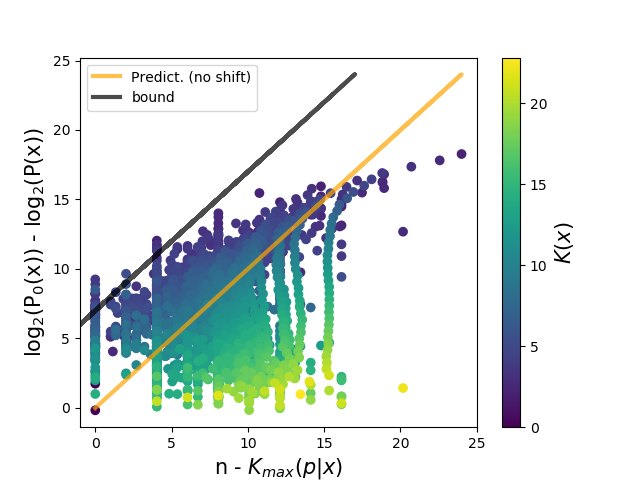
By combining with Eq. (2), the bound (3) can be rewritten in two complementary ways. Firstly, a lower bound on $P(x)$ can be derived of the form:

$$P(x)\geq 2^{-K(x|f,n)-[n-K(p|f,n)]+\mathcal{O}(1)}$$ (7)

$\forall p\in f^{-1}(x)$ which complements the simplicity bias upper bound (1). This bound is tightest for $K_{\text{\rm max}}(p|n)$.

In Ref.  Dingle et al. (2018) it was shown that $P(x)\leq 2^{-K(x|f,n)+\mathcal{O}(1)}$ by using a similar counting argument to that used above, together with a Shannon-Fano-Elias code procedure. Similar results can be found in standard works Li and Vitanyi (2008); Gács (1988). A key step is to move from the conditional complexity to one that is independent of the map and of $n$. If $f$ is simple, then the explicit dependence on $n$ and $f$ can be removed by noting that since $K(x)\leq K(x|f,n)+K(f)+K(n)+\mathcal{O}(1)$, and $K(x|f,n)\leq K(x)+\mathcal{O}(1)$ then $K(x|f,n)\approx K(x)+\mathcal{O}(1)$. In Eq. (1) this is further approximated as $K(x|f,n)+\mathcal{O}(1)\approx a\tilde{K}(x)+b$, leading to a practically useable upper bound. The same argument can be used to remove explicit dependence on $n$ and $f$ for $K(p|f,n)$.

If we define a maximum randomness deficit $\delta_{\rm max}(x)=n-K_{\text{\rm max}}(p|n)$, then this tightest version of bound (7) can be written in a simpler form as

$$P(x)\geq 2^{-a\tilde{K}(x)+b-\delta_{\rm max}(x)+\mathcal{O}(1)}$$ (8)

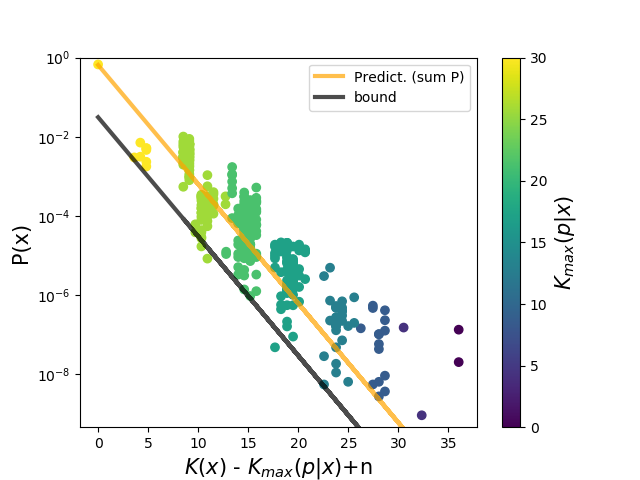
In Figs. 1 (d-f) we plot this lower bound for all three maps studied. Throughout the paper, we use a scaled complexity measure, which ensures that $\tilde{K}(x)$ ranges between $\approx$0 and $\approx$$n$ bits, for strings of length $n$, as expected for Kolmogorov complexity. See Methods for more details.

When comparing the data in Figs. 1 (d-f) to Figs. 1 (a-c), it is clear that including the input complexities reduces the spread in the data for RNA and the FST, although for the perceptron model the difference is less pronounced. This success suggests using the bound (8) as a predictor $P(x)\approx 2^{-K(x|f,n)-\delta_{\rm max}(x)}$, with the additional constraint that $\sum_{x}P(x)=1$ to normalise it. As can be seen in Figs. 1 (d-f), this simple procedure works reasonably well, showing that the input complexity provides additional predictive power to estimate $P(x)$ from some very generic properties of the inputs and outputs.

A second, complimentary way that bound (3) can be expressed is in terms of how far $P(x)$ differs from the simplicity bias bound (1):

$$\left[\log_{2}(P_{0}(x))-\log_{2}(P(x))\right]\leq[n-K(p|f,n)]+\mathcal{O}(1)$$ (9)

where $P_{0}(x)=2^{-K(x|f,n)}\approx 2^{-a\tilde{K}(x)+b}$ is the upper bound (1) shown in Figs 1 (a-c).

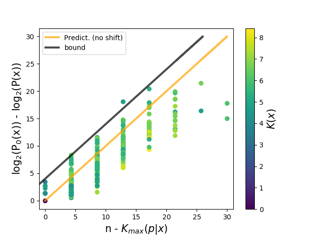
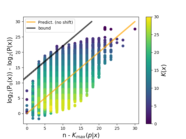
For a random input $p$, with high probability we expect $K(p|f,n)=n+\mathcal{O}(1)$ Li and Vitanyi (2008). Thus, eqs. (7) and (9) immediately imply that large deviations from the simplicity bias bound (1) are only possible with highly non-random inputs with a large randomness deficit $\delta_{\rm max}(x)$.

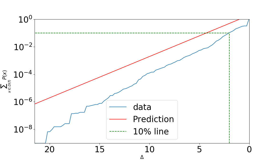
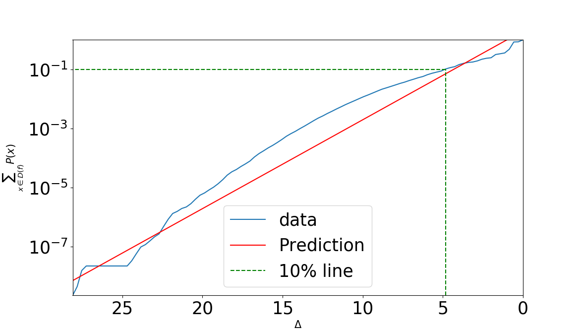
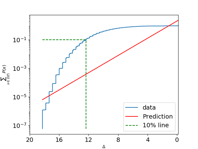
In Fig. 2(a)-(c) we directly examine bound (9), showing explicitly the prediction that a drop of probability $P(x)$ by $\Delta$ bits from the simplicity bias bound ( 1) corresponds to a $\Delta$ bit randomness deficit in the set of inputs.

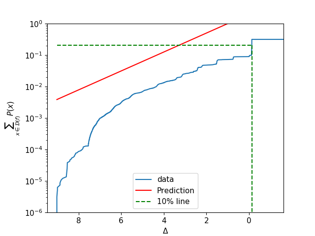
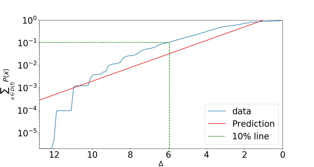
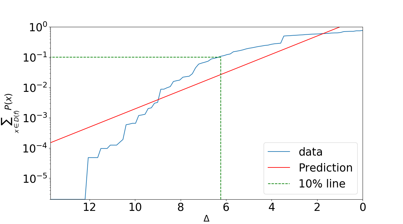
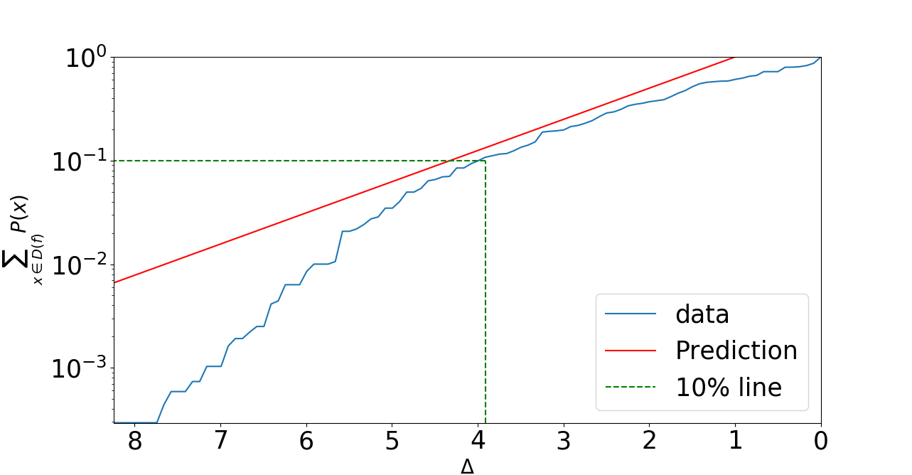
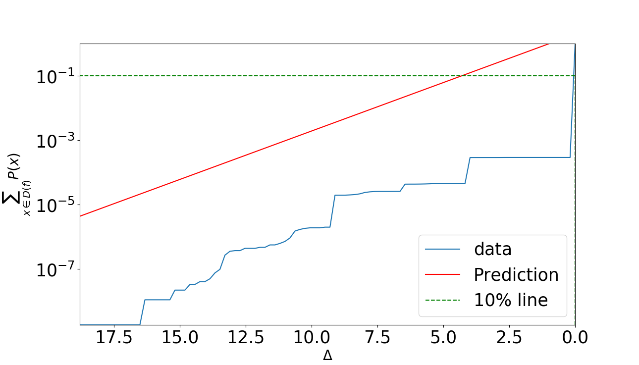
Simple counting arguments can be used to show that the number of non-random inputs is a small fraction of the total number of inputs Chaitin (1974). For example, for binary strings of length $n$, with $N_{I}=2^{n}$, the number of inputs with complexity $K=n-\delta$ is approximately $2^{-\delta}N_{I}$. If we define a set $\mathcal{D}(f)$ of all outputs $x_{i}$ that satisfy $(\log_{2}(P_{0}(x_{i}))-\log_{2}(P_{(}x_{i})))\geq\Delta$, i.e. the set of all outputs for which $\log_{2}P(x)$ is at least $\Delta$ bits below the simplicity bias bound (1), then this counting argument leads to the following cumulative bound:

$$\sum_{x\in\mathcal{D}(f)}P(x)\leq 2^{-\Delta+1+\mathcal{O}(1)}$$ (10)

which predicts that, upon randomly sampling inputs, most of the probability weight is for outputs with $P(x)$ relatively close to the upper bound. There may be many outputs that are far from the bound, but their cumulative probability drops off exponentially the further they are from the bound because the number of simple inputs is exponentially limited. Note that this argument is for a cumulative probability over all inputs. It does not predict that for a given complexity $K(x)$, that the outputs should all be near the bound. In that sense this lower bound is not like that of the original coding theorem which holds for any output $x$.

Figure 3: The cumulative probability versus the distance from the bound $\Delta$ correlates with the the cumulative bound (10) (red line) for (a) L=15 RNA and (b) L=30 FST (c) Perceptron. (d) fully connected 2 layer neural network from Valle-Pérez et al. (2018), (e) coarse-grained ordinary differential equation map from Dingle et al. (2018), (f) Ornstein-Uhlenbeck financial model from Dingle et al. (2018), (g) L-systems from Dingle et al. (2018), (h) simple matrix map from Dingle et al. (2018). The solid red line is the prediction $2^{-\Delta+1}$ from Eq. (10), the dashed line denotes $10\%$ cumulative probability.

,

Bound (10) does not need an exhaustive enumeration to be tested. In Fig. 3 we show this bound for a series of different maps, including many maps from Dingle et al. (2018). The cumulative probability weight scales roughly as expected, implying that most of the probability weight is relatively close to the bound (at least on a log scale).

What is the physical nature of these low complexity, low probability outputs that occur far from the bound? They must arise in one way or another from the lower computational power of these maps, since they don’t occur in the full AIT coding theory. Low complexity, low probability outputs correspond to output patterns which are simple, but which the given computable map is not good at generating.

In RNA it is easy to construct outputs which are simple but will have low probability. Compare two $L=15$ structures $S_{1}=$((.(.(…).).)). and $S_{2}=$.((.((…)).))., which are both symmetric and thus have a relatively low complexity $K(S_{1})=K(S_{2})$ $=21.4$. Nevertheless they have a significant difference in probability, $P(S_{2})/P(S_{1})\approx 560$ because $S_{1}$ has several single bonds, which is much harder to make according to the biophysics of RNA. Only specially ordered input sequences can make $S_{1}$, in other words they are simple, with $K_{\text{\rm max}}(p|n)=8.6$. By contrast, the inputs of $S_{2}$ are much higher at $K_{\text{\rm max}}(p|n)=21.4$ because they need to be constrained less to produce this structure. This example illustrates how the system specific details of the RNA map can unfavourably bias away from some outputs due to a system specific constraint.

Similar examples of system specific constraint for the FST and perceptron can be found in the SI. We hypothesise that such low complexity, low probability structures highlight specific non-universal aspects of the maps, and extra information (in the form of a reduced set of inputs) are needed to generate such structures.

In conclusion, it is striking that bounds based simply on the complexity of the inputs and outputs can make powerful and general predictions for such a wide range of systems. Although the arguments used to derive them suffer from the well known problems – e.g. the presence of uncomputable Kolmogorov complexities and unknown ${\mathcal{O}}(1)$ terms – that have led to the general neglect of AIT in the physics literature, the bounds are undoubtably successful. It appears that, just as is found in other areas of physics, these relationships hold well outside of the asymptotic regime where they can be prove to be correct. This practical success opens up the promise of using such AIT based techniques to derive other results for computable maps from across physics.

Many new questions arise. Can it be proven when the $\mathcal{O}(1)$ terms are relatively unimportant? Why do our rather simple approximations to $K(x)$ work? It would be interesting to find maps where these classical objections to the practical use of AIT are important. There may also be connections between our work and finite state complexity Calude et al. (2011) or minimum description length Grünwald and Roos (2019) approaches. Progress in these domains should generate new fundamental understandings of the physics of information.